A Smart Terrain Identification Technique Based on Electromyography, Ground Reaction Force, and Machine Learning for Lower Limb Rehabilitation

Abstract

Automatic terrain classification in lower limb rehabilitation systems has gained worldwide attention. In this field, a simple system architecture and high classification accuracy are two desired attributes. In this article, a smart neuromuscular–mechanical fusion and machine learning-based terrain classification technique utilizing only two electromyography (EMG) sensors and two ground reaction force (GRF) sensors is reported for classifying three different terrains (downhill, level, and uphill). The EMG and GRF signals from ten healthy subjects were collected, preprocessed and segmented to obtain the EMG and GRF profiles in each stride, based on which twenty-one statistical features, including 9 GRF features and 12 EMG features, were extracted. A support vector machine (SVM) machine learning model is established and trained by the extracted EMG features, GRF features and the fusion of them, respectively. Several methods or statistical metrics were used to evaluate the goodness of the proposed technique, including a paired-t-test and Kruskal–Wallis test for correlation analysis of the selected features and ten-fold cross-validation accuracy, confusion matrix, sensitivity and specificity for the performance of the SVM model. The results show that the extracted features are highly correlated with the terrain changes and the fusion of the EMG and GRF features produces the highest accuracy of 96.8%. The presented technique allows simple system construction to achieve the precise detection of outcomes, potentially advancing the development of terrain classification techniques for rehabilitation.

1. Introduction

Applying intelligent rehabilitation techniques, such as rehabilitation robots [1,2,3,4,5,6,7] or in-home rehabilitation systems based on wearable sensors [8,9,10,11,12], to help people suffering from limited mobile ability to perform physical rehabilitation is of significance. Such intelligent techniques alleviate the shortage of physical therapists and realize data monitoring for more accurate evaluations on patients [13,14,15,16], and thus have become a new trend in recent years. The traditional scenario for lower limb rehabilitation is level walking. In recent years, terrain classification techniques enable wearable assistant systems to recognize more terrains, which allows patients to perform rehabilitation training in more complex scenarios, and therefore has aroused wide attention [17,18,19]. Among all terrains, uphill, level ground, and downhill are the three most common terrains in daily life, and thus are widely investigated in the study of terrain identification [19,20,21,22].

The input signals of these kinds of rehabilitation-driven systems for terrain classification include kinematics information (e.g., inertial measurement units (IMUs)), kinetics information (e.g., ground reaction force and interaction force), and electromyography (EMG) signals [23,24,25,26,27]. Using the input signals mentioned above, increasing efforts have been made for classifying different terrains. For example, in [28], five time-domain features of the EMG signals from eight muscles on the thigh were extracted and analyzed. Ramp and level walking were classified for thirteen healthy participants and the average classification accuracy for all terrains was 92.9%. In [27], signals from 13 IMUs on the robotic legs of six transfemoral amputee subjects were collected and used to classify different terrains and an average accuracy of 81.2% was reached in recognizing ramp and level ground. In [22], the authors proposed a terrain identification method, namely muscle synergies, based on the EMG signals from twelve muscles. The data from seven able-bodied participants were collected and were classified as level ground and ramp with an average accuracy of 83.8%. However, in general, using a single sensor type lacks in a comprehensive detection of the bodily changes of the user, and thus is not adequate for high-accuracy terrain recognition [17,19].

To obtain multi-dimensional information, the fusion of multi-sensor data, together with machine learning-based sensor fusion algorithms, is widely used in terrain identification in recent years. Some studies report the integrated use of accelerometers, angle sensors, kinematic data captured by camera, EMG signals, etc., to differentiate terrains [20,21,29,30,31]. For example, in [32], nine EMG and six ground reaction force (GRF) sensors were utilized, based on which five terrains were identified continuously in four gait phases using the linear discriminant analysis (LDA) and support vector machine (SVM) methods, and the ramp–level ground classification accuracy in this work was averaged at 97.73%. In [20], four healthy subjects performed walking activities on uphill, level ground and downhill, and a high average terrain classification accuracy of 93.4%, based on the Bayesian LDA, was achieved through developing a technique consisting of an interaction force sensor, four EMG sensors, four GRF sensors, and a position sensor. In [21], the data from seven healthy subjects collected by seven EMG sensors and two accelerometers were obtained and used to classify the terrain transition from level ground to stairs or ramp; from this, the classification performance of the EMG and accelerometer signal was compared and discussed, proving that the fusion of both signals may contribute to a more robust classification. In [19], a terrain identification-enabled exoskeleton system which integrated only two attitude and heading reference system (AHRS) sensors and three GRF sensors was designed, tested by three healthy subjects and successfully identified ramp and level ground, with a mean accuracy of 97.77%. The number and categories of the applied sensors and the classification accuracy of the above studies, along with some other relevant studies [17,33,34,35], are summarized in Figure 1.

We can infer from Figure 1 that fruitful results have been made by relevant studies in order to obtain a robust identification accuracy and low complexity at the same time. Nevertheless, a multi-sensory terrain identification system utilizing neuromuscular signals such as EMG, which has proved to have a better performance in interpreting and predicting the intention of the user compared to mechanical signals [28,36,37,38], with both a simple structure and high detection accuracy, has not been reported yet. To fill the gap, in this article, a smart neuromuscular–mechanical fusion terrain classification technique based on GRF detection, EMG and machine learning is presented. Here, only four sensors, including two EMG sensors attached to two muscles (tibialis anterior and soleus) and two GRF sensors placed at the hallux and heel, were used for classifying uphill, level ground and downhill. The collected signals are preprocessed and analyzed to draw the typical profiles of the EMG and GRF, based on which novel features reflecting the changing patterns of the EMG and GRF were selected for the support vector machine (SVM) machine learning algorithm to classify the terrains. To verify the proposed technique, standard experimental procedures compatible with relevant studies on different terrains were performed. Comparisons were made using the EMG and GRF information, respectively, and the combination of them to evaluate the effectiveness of the sensors’ fusion. A paired t-test and Kruskal–Wallis test were applied to evaluate the correlation of the selected features and terrain changes. Ten-fold cross-validation accuracy together with sensitivity and specificity were used to evaluate the goodness of the SVM machine learning model. An overview process of this work is conceptually described in Figure 2.

The paper is organized as follows. In Section 2, we explain the methodology of the experiment setup, data pre-processing, feature extraction, establishment of SVM model and evaluation of the selected features and the classifier. In Section 3, the experimental results are demonstrated and discussed, including the EMG and GRF profiles, statistical features of the different terrains and the performance of the SVM model.

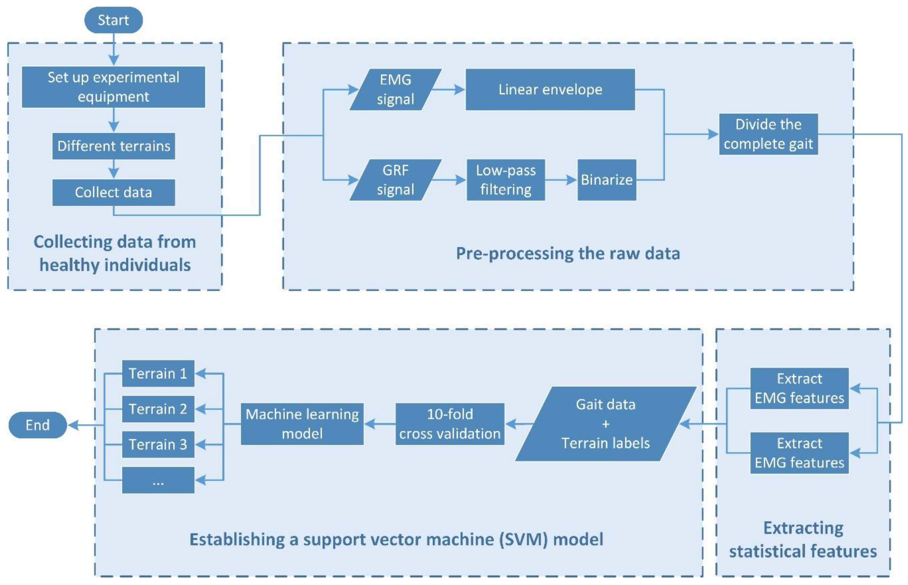
2. Methodology

In order to accurately classify the terrain conditions, the features of the EMG and GRF in the different terrains were studied and extracted by the following steps, as shown in Figure 3:

• Collecting data from healthy individuals;
• Pre-processing the raw data;
• Extracting the statistical features;
• Establishing an SVM model.

Correlation analysis and statistical metrics will be used to examine the proposed method. The above steps will be discussed in detail in the following sections.

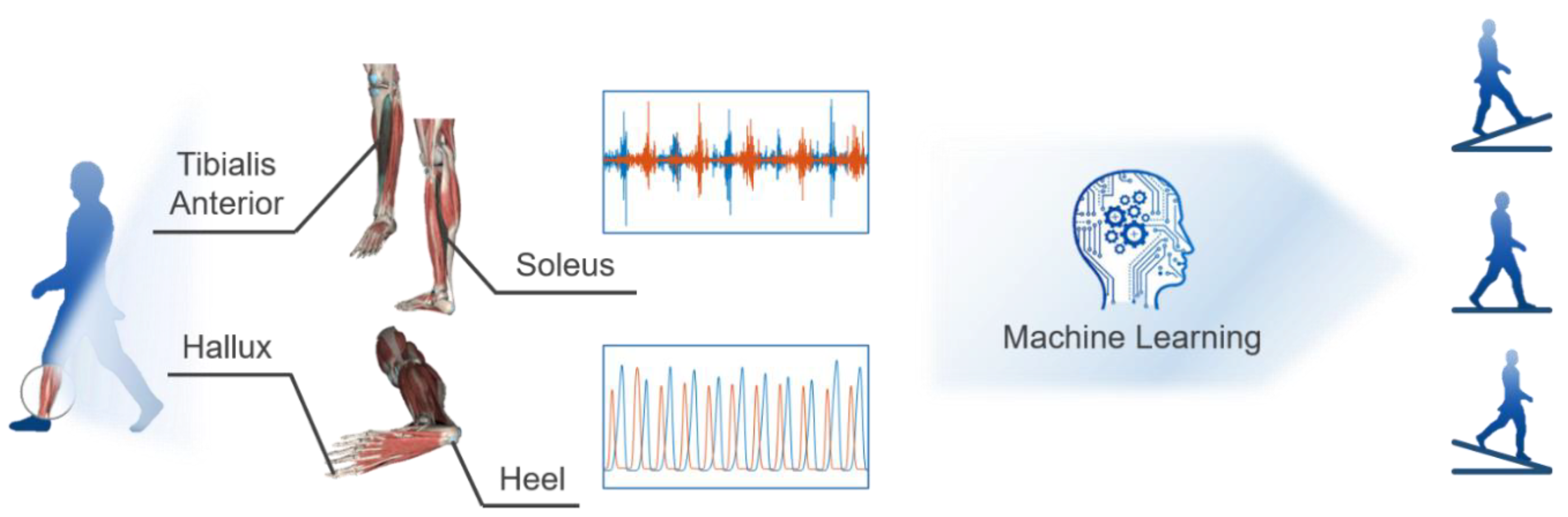
2.1. Experiment Setup

Ten healthy individuals (6 male and 4 female) were recruited as volunteers to participate in the experiment. They had no previous medical history of neurological and muscular diseases. Subjects’ consent was obtained before the experiment. Ethical approval was obtained from the Shijiazhuang Central Hospital, Shijiazhuang, Hebei Province, China. Their physical body conditions are shown in

Table 1. Mean and standard deviation of the physical body conditions of the 10 volunteers.

Height/cm	Weight/kg	Age
175.70 ± 6.63	66.20 ± 9.19	20.80 ± 1.40

.

A pair of distal antagonistic muscles, tibialis anterior (TA) and soleus (SL), were selected in this experiment because the EMG signals of the distal muscles show lower inter-subject variability than the proximal [39]. The skin of the selected muscles was shaved and cleaned with 75% alcohol before the experiment [40]. Three Ag-AgCl electrodes of 5 mm in diameter, including a reference and two differential amplification ones [41], were attached to the ankle and the surface of the selected muscles, respectively. The location and distance of the electrodes are referred to in [42]. The EMG signals were acquired by a two-channel EMG device.

Two circular force sensing resistors (FSR), ranging from 20 to 20,000 g, were attached to the flat area of the heel and hallux to collect the GRF signal for the stride division [43]. The resistance change of the FSRs was linearly converted to a voltage change by proportional operational amplifiers and then converted to digital signals by analog-to-digital converters (ADCs) embedded in STM32F103C8T6. Both the EMG and GRF signals were sampled at a frequency of 2000 Hz, which is adequate for terrain classification compared with other studies, and transmitted to PC via Bluetooth. A JavaScript script was written, which automatically obtained the system time and added it to the end of each message sent to the PC. Finally, the EMG and GRF signals with the same particular timestamp were aligned, and then all of the synchronized datapoints were used for further analysis.

The participants were instructed to walk at comfortable speeds according to their walking habits. It is worth noting that the EMG profiles would change slightly when walking speeds varied, i.e., shifting less than 10% and 1% in peak amplitude and peak timing, within a certain range around normal walking speed [30,44], which are acceptable for classifying three to five different terrains, and therefore the developed protocol is also applied in other relevant studies [19,32]. When the start command was issued, the participant stepped out on the leg with the device. Data acquisition started at the first heel strike. The participants were instructed to walk a forty-meter flat ground four times, and then walked back and forth twenty times on a slope with a length of 5 m angled at 5.2 degrees. Similar ramp angle degrees are also found in other relevant studies and they are summarized in

Table 2. Ramp angles selected in other relevant studies and comparison with our work.

Relevant Work	Ramp Angle
[22]	4.78 degree
[27]	10 degree
[31]	10 degree
[19]	12 degree
[35]	8.5 degree
This work	5.2 degree

for comparison with our work [19,22,27,31,35].

The participants were fully warmed-up to familiarize themselves with the protocol to ensure they walk naturally with the measurement device, and rested for 15 min after each level walking task and 5 consecutive slope walking tasks in order to prevent muscle fatigue [45]. At the end of all the trials, the participants performed a maximum isometric voluntary contraction (MIVC) for the EMG normalization.

2.2. Data Pre-Processing

A total of 767,324 synchronized EMG and GRF datapoints in 1918 strides, including 640 uphill, 704 level walking and 574 downhill, were selected. The pre-processing of the EMG and GRF signals was performed in MATLAB.

The raw EMG signal needs to be filtered before it can be used for further analysis because it is interfered with by noise. For the high-frequency region, most of the energy of the EMG signal mainly concentrates within 0–500 Hz [46], and the high-frequency region (500–1000 Hz) of the EMG signal is likely to be interfered with by aliasing, according to [47,48]. For the low-frequency region, the frequency range of the movement artifacts, which is a type of noise caused by the movement of the cable and the interface between the detection surface of the electrode and the skin, is typically 1–10 Hz [49]. Therefore, the raw EMG signal was filtered by a finite impulse response (FIR) bandpass filter with cutoff frequencies of 10 (low) and 500 Hz (high) [41,50,51,52].

After denoising, we applied normalization to the EMG amplitude to reduce the inter-subject variability of the EMG signals. The widely applied normalization references include the peak of EMG from the ensemble average, the mean of the ensemble average, and maximal isometric voluntary contraction (MIVC) [53]. In this work, a MIVC was chosen because it is less likely to be affected by joint kinematics like knee or ankle flexion. Furthermore, different levels of MIVC have been researched, and 50% has been proven to be an optimal point as it is easier to be reached and maintained by the experiment participants, according to [54,55]. Hence, the EMG amplitude in this work was normalized by 50% MIVC. Furthermore, we also calculated the linear envelope (LE) of the EMG signal, which is an intuitive processing method of EMG reflecting the muscle force level [56]. Specifically, a full-wave rectification and a lowpass filter with a cutoff frequency of 3 Hz were used to obtain the LE, as previous research has evidenced the ability of the 3 Hz cutoff frequency to provide good relations with muscle force [56,57,58,59,60].

The GRF data was normalized to the body weight of each participant [61]. An important function of the GRF signal is for segmenting the collected data sequence into complete stride sequences. Here, the GRF data (without normalization) were binarized with a threshold of 300 g [43]. The timing of the binarized data, changing from 0 to 1, of the heel was considered as the timing of the heel strike (HS), and the interval of the two consecutive HSs was seen as the duration of a complete gait [62,63]. In this way, the GRF and EMG data were segmented into a group of strides.

Finally, we generate the profiles of the EMG, LE and GRF curves in each stride by calculating the ensemble average of the signals from all the participants. The ensemble average is obtained by the following procedure: Firstly, the stride time divided by the HS was normalized to 100%, and then all the EMG, LE and GRF curve data at each consecutive 1% of the normalized stride time were selected and averaged, producing the ensemble average [56]. Finally, a standard deviation (SD) band of ±1 about the average was calculated to quantify the variability of each stride [56].

2.3. Feature Extraction

After the signal was pre-processed, the noise was attenuated while the stride segments were obtained. However, the sequence data of these segments could not be directly fed into the SVM model due to the large computation cost and the poor correlation between the class and the original sequence data, which would have negatively affected the classification performance. Instead, some statistical features extracted from the pre-processed signal were the appropriate choices for the input of the SVM model.

A total of 21 statistical features, including 12 EMG features and 9 GRF features, in each step were extracted to classify the terrain. The feature symbols used in this paper and their specific meanings are shown in

Table 3. Extracted features of the EMG and GRF, where i is the index of EMG filtered amplitude and N is the length of the sequence in a stride.

Symbol	The Meaning of the Features
GRF-Based
Hallux Max	The max value of hallux GRF
Heel Max	The max value of heel GRF
Max T	The time interval between the two peaks
Hallux ON	The duration of Hallux GRF above the threshold
Heel ON	The duration of Heel GRF above the threshold
Hallux OFF	The duration of Hallux GRF below the threshold
Heel OFF	The duration of Heel GRF below the threshold
Start T	The time interval between Hallux ON and Heel ON
End T	The time interval between Hallux OFF and Heel OFF
EMG-Based
TA Peak	The peak value of the TA linear envelope
TA MAV	$\mathrm{MAV}\mathrm{of}\mathrm{the}\mathrm{TA}\mathrm{EMG},MAV=\frac{1}{N}{\displaystyle {\sum }_{i=1}^N\left|x_i\right|}$
TA STD	$\mathrm{STD}\mathrm{of}\mathrm{the}\mathrm{TA}\mathrm{EMG};STD=\sqrt{\frac{{\displaystyle {\sum }_{i=1}^N{(x_i-\overline{x})}^2}}{N}}$
TA RMS	$\mathrm{RMS}\mathrm{of}\mathrm{the}\mathrm{TA}\mathrm{EMG};RMS=\sqrt{\frac{{\displaystyle {\sum }_{i=1}^N{x}_i{}^2}}{N}}$
TA WL	WL of TA EMG; $WL={\displaystyle {\sum }_{i=2}^N|\Delta x_i|}$, where Δxi = xi − xi−1
TA 80	The value of the TA linear envelope at 80% gait
SL Peak	The peak value of the SL linear envelope
SL MAV	MAV of the SL EMG, $MAV=\frac{1}{N}{\displaystyle {\sum }_{i=1}^N\left|x_i\right|}$
SL STD	STD of the SL EMG; $STD=\sqrt{\frac{{\displaystyle {\sum }_{i=1}^N{(x_i-\overline{x})}^2}}{N}}$
SL RMS	RMS of the SL EMG; $RMS=\sqrt{\frac{{\displaystyle {\sum }_{i=1}^N{x}_i{}^2}}{N}}$
SL WL	WL of SL EMG; $WL={\displaystyle {\sum }_{i=2}^N|\Delta x_i|}$, where Δxi = xi − xi−1
SL 25	The value of the SL linear envelope at 25% gait

. These features can be divided into three categories as follows:

• Force and time features extracted from the GRF curve. Such features reflect the variation and relationship of the two GRF measures during a stride or between two consecutive strides and they are depicted in Figure 4a.
• Time-domain features extracted from the filtered EMG data, including the mean absolute value (MAV), standard deviation (STD), root mean square (RMS), and waveform length (WL), which are broadly used features, such as in [28,49]. Such features reflect the overall activation level of the muscle in a stride.
• Muscle force features extracted from the EMG and LE, including the TA peak, TA 80, SL peak, SL 25. Such features reflect the muscle force level at a particular timing of a stride and they are depicted in Figure 4b.

2.4. Establishment of SVM Model

The machine learning model—the support vector machine (SVM)—has been widely used for the pattern recognition or classification of the EMG signal [64,65]. The basic idea behind the SVM is to construct an optimal hyperplane [66], which can be used to classify linear separable patterns. Non-linear separable patterns are mapped into higher-dimension space through a kernel function, so that the patterns become linearly separable [67]. The kernel function selected in this paper was the radial basis function (RBF) kernel, which has a good classification performance for multi-classifiers with a small margin between each of the two classes [68].

The establishment of the SVM model in this paper is described as follows: The features and labels of the selected steps were used as the input vector of the model, and a ten-fold cross-validation method [64,69] was applied to train the SVM model. In this method, all of the samples were split equally into 10 groups while ensuring the proportion of each class in each group remained unchanged. Then, one group was used for testing and the other nine groups were used for training. The process above was iterated until all groups had been treated as the testing set.

2.5. Evaluation of the Selected Features and the SVM Model

To evaluate the goodness of our selected features and the classification performance of the SVM model, we adopt several metrics and analysis methods for the evaluation.

The Kruskal-–Wallis test by ranks was applied on each feature, which is a non-parametric method for determining whether three or more independent groups of equal or different sample sizes are the same or different on some variable of interest [70,71]. This test showed if there is a significant difference between the three terrains for each feature. Furthermore, to evaluate the statistical difference between each two terrains, the paired t-test, a statistical procedure used to determine whether the mean difference between two sets of observations is zero [45], was used after a Kolmogorov–Smirnov (KS) test, ensuring that the features in each class obey a Gaussian distribution.

For the SVM model, four kind of indexes, i.e., average accuracy, confusion matrix, sensitivity and specificity, are used to evaluate the classification performance. The average accuracy (acc) of the SVM model is defined as

$$acc=\frac{N_c}{N_{total}}\times 100\%$$

(1)

where $N_c$ is the number of correctly classified events, and $N_{total}$ is the total number of the test events. Here, the test events mean all the applied test set data in the ten-fold cross-validation procedure.

The confusion matrix Q is used to better quantify the specifics of the classification [19], which is defined in this paper as follows:

$$Q=\left[\begin{array}{c}\begin{array}{ccc}{q}_{11}& q_{12}& q_{13}\end{array}\\ \begin{array}{ccc}{q}_{21}& q_{22}& q_{23}\end{array}\\ \begin{array}{ccc}{q}_{31}& q_{32}& q_{33}\end{array}\end{array}\right]$$

(2)

where the element of the confusion matrix is defined as

$$q_{ij}=\frac{p_{ij}}{p_{total,i}}\times 100\%$$

(3)

where p_ij is the number of samples of the ith terrain that are identified as the jth terrain, and p_total,i is the total number of samples of the ith terrain. The elements on the diagonal present the classification accuracy and the others show the errors.

In addition to accuracy, the calculation of sensitivity and specificity is beneficial for evaluating the SVM model’s performance in binary classification problems [72]. They are defined as follows:

$$SEN=\frac{TP}{TP+FN}$$

(4)

$$SPE=\frac{TN}{TN+FP}$$

(5)

where SEN and SPE denote sensitivity and specificity, and TP, TN, FP, FN are defined as follows (

Table 4. The definitions of TP, TN, FP and FN.

	Actual Value	Positive	Negative
Prediction
Positive		TP	FP
Negative		FN	TN

):

In this work, when considering one terrain as the positive value, the other two terrains are seen as the negative values, and therefore three sensitivities and specificities are calculated when taking each terrain as the positive value in turn.

3. Results and Discussion

The results and discussions mainly consist of three parts:

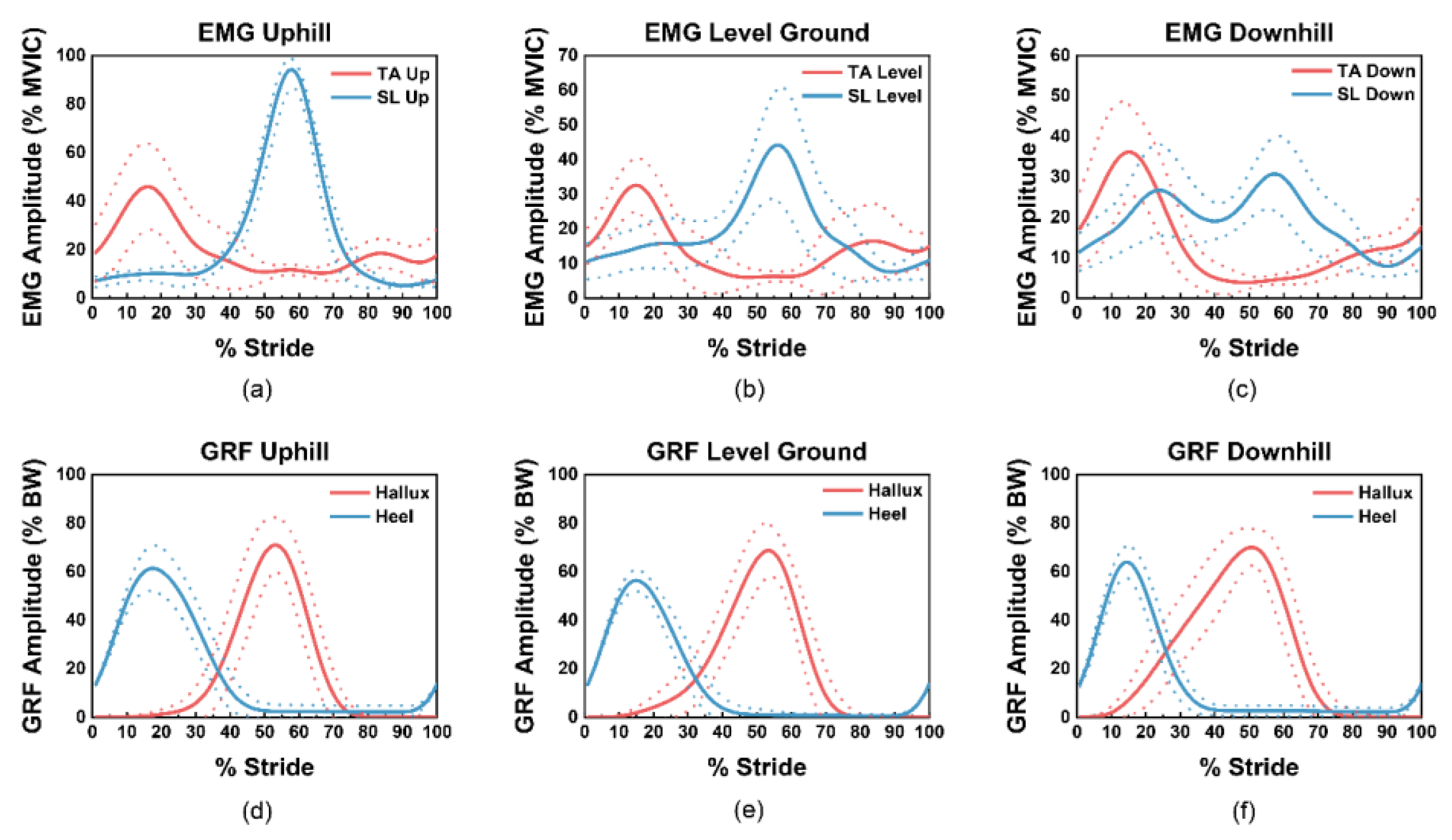
• The profile of the EMG, LE and GRF curves;
• The comparison and explanation of the differences between the extracted features in the different terrains;
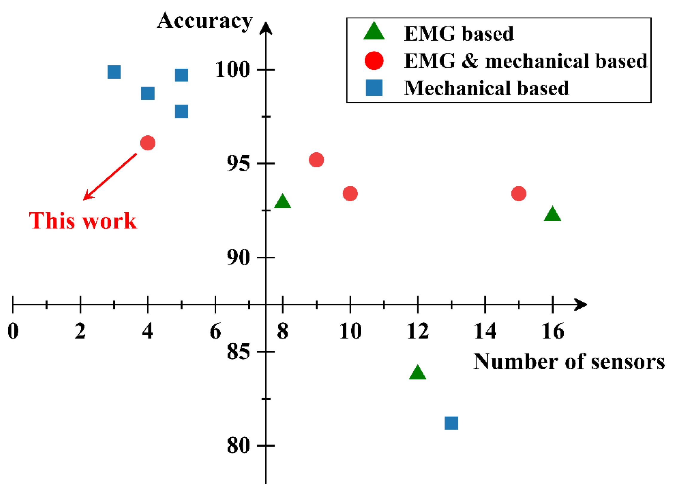
• The classification performance of the SVM model and the discussion on sensor fusion.

3.1. EMG and GRF Profiles

The ensemble average of the EMG of the TA and SL and the GRF curve of the heel and the hallux of two representative subjects randomly selected from 10 subjects are plotted in Figure 5. The solid line in Figure 5 is the ensemble average, whereas the dashed line is the ±1 standard deviation (SD) band, and the distance between them represents the stride-to-stride and inter-subject variability at different moments of the gait. It can be seen that, generally, the SD of the curve will be larger at the peak, where greater force is applied by humans. It can be concluded that although there are some differences between the different strides, individuals and terrains, both the EMG and GRF follow similar profiles [39,56,73]. Taking the GRF signal as a reference, the EMG–LE profile reveals the state of muscle exertion in a complete gait. For the TA, two peaks can be observed. The TA generates the peak at about 25% of the gait cycle to lower the foot to the ground soon after the HS. After the toe-off (TO), at about 80% gait, a smaller peak is generated for the foot clearance, resulting in ankle dorsiflexion. For the SL, the main feature is a significant peak at about 60% gait when the SL contracts and generates the impulse of energy to push-off. When walking downhill, the SL also plays a minor roll during midstance, mainly to maintain a balanced gait, which results in the rise at 25% gait when walking downhill. It is worth noting that the discussion above is the basis of selecting the statistical features of the EMG, which will be discussed in detail in Section 3.2. In addition, Figure 5b shows the EMG profile of the TA and SL when walking on level ground, which is consistent with the standard profile of these two muscles during level walking presented in [56], and highlights the correctness of the experimental setup and data pre-processing. Section 3.3 will further validate the classification performance of our proposed technique.

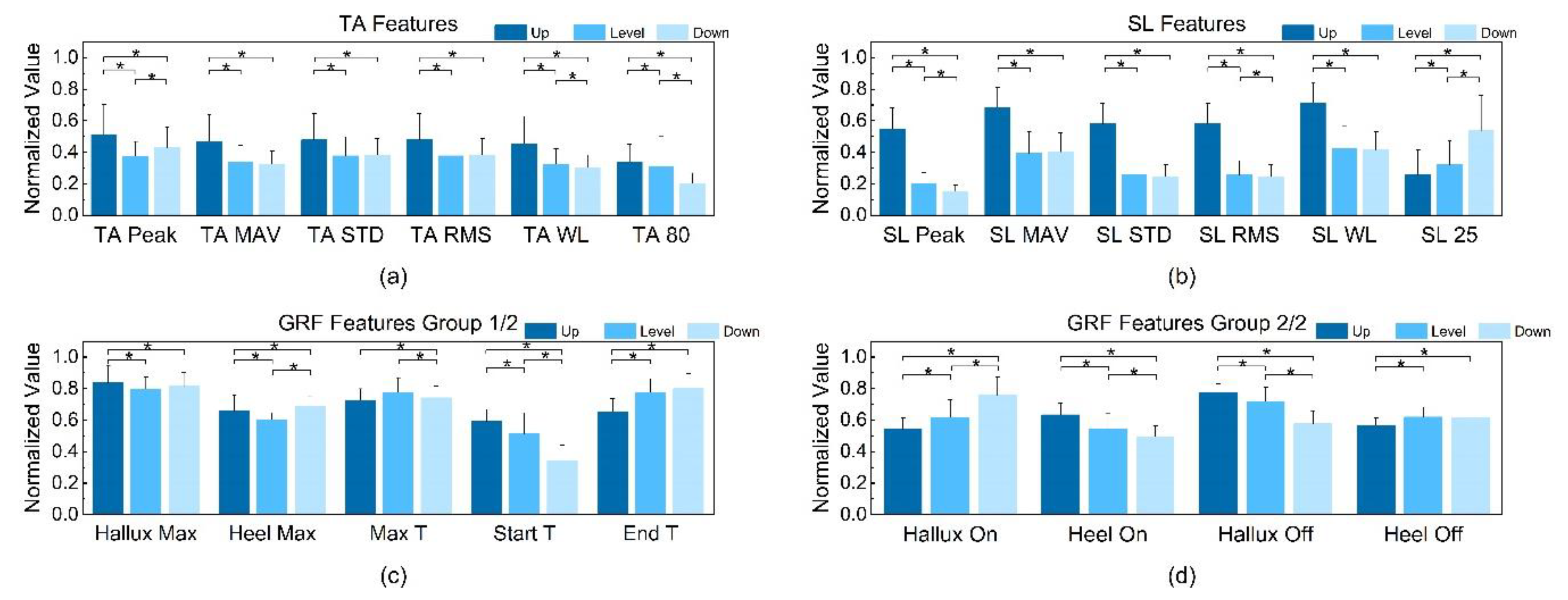
3.2. Statistical Features in Different Terrains

The EMG and GRF profiles reveal the overall difference qualitatively, and the statistical features extracted in Table 3 quantitatively describe the difference between the EMG signal and GRF signal in the different terrains. Figure 6 shows the average and normalized value of each feature in each terrain. The following subsections will explain the biomechanical reasons for the variability of the features in the different terrains.

3.2.1. TA EMG

The peak, mean absolute value (MAV), standard deviation (STD), root mean square (RMS), and waveform length (WL) of the TA are significantly larger for uphill than for flat and downhill, indicating that the TA is more active during uphill. This is because more efforts are made in order to overcome gravity and lift the body up when walking uphill [74]. In addition, the TA peak increases from level to downhill. The reason for that may be that the TA contracts more to resist the downward trend when walking downhill, resulting in more contraction of the TA, which aligns with the profile presented in [75]. Meanwhile, the feature “TA 80” decreases when going downhill because the gravity helping the foot clearance at 80% stride reduces the activity of the TA.

3.2.2. SL EMG

The SL peak has the most significant difference among the three types of terrains, decreasing from uphill, to level, to downhill. This is because the push-off force generated by the SL needs to overcome the effect of gravity when walking uphill to make the body move forward, while the activity is the opposite when walking downhill. The MAV, WL and other statistical data follow a similar rule as the TA, indicating that muscle activity is generally higher when walking uphill. In addition, the co-contraction of the SL with the TA to stabilize the gait when going downhill makes the “SL 25” increase. The above phenomenon is also observed in [76].

3.2.3. Ground Reaction Force

From uphill to downhill, the features “Start T” and “Heel ON” are decreasing, while “Hallux ON” and “End T” are increasing, which means that the time interval between the front and rear foot landing is shorter during downhill, while the time taken for the front foot to grip the ground is longer. A similar discipline reporting a lower duty factor in foot strike was also observed in [74]. This can resist the tendency of slipping downhill during the stance phase and make the gait stable, whereas in uphill, the shorter burst of the front foot helps to achieve sufficient thrust to move forward.

The significant differences (p < 0.05) tested by the paired t-test of the features between each pair of terrains are also shown in Figure 6. The p-values of the KS test, Kruskal–Wallis test and paired t-test are shown in Table S1 in the Supplementary Materials and the distribution of all the features in each terrain were Gaussian (p > 0.05). Here, all the features pass the Kruskal –Wallis test (p < 0.05), and significant differences (p < 0.05) between at least two pairs of terrains were observed in the features we selected, which indicates that all the features contributed to correctly classifying the terrains positively. In addition, significant differences between all the three pairs of the terrains were observed in the four features we proposed in the EMG feature set, i.e., the TA peak, SL peak, TA 80 and SL 25, as shown in Figure 6, which indicates that the features we proposed in this work were more correlated with the terrains compared with the conventional EMG time-domain features. The p-values presented here proved that the features selected in this work were highly correlated with the terrain labels, which potentially improved the performance of the classifier. The following section will evaluate the performance of the SVM model utilizing these features.

3.3. Training Performance of SVM and Comparison between the EMG and GRF Features

The extracted features were set as inputs for the machine learning algorithm. Here, the GRF and EMG are used separately to train the model first, and then the combination of them is employed. The average and standard deviation of the overall accuracy, sensitivity and specificity of the different selected sets of features are shown in

Table 5. The average and standard deviation (SD) of the accuracy, sensitivity and specificity of the model using different sets of features.

		GRF	EMG	GRF + EMG
Accuracy ± SD		80.96% ± 6.17%	89.93% ± 3.63%	96.76% ± 1.57%
SEN ± SD	Uphill	83.44% ± 5.47%	95.00% ± 3.28%	98.59% ± 1.15%
	Level ground	78.68% ± 7.36%	88.49% ± 4.62%	96.87% ± 1.62%
	Downhill	80.99% ± 10.25%	86.04% ± 6.97%	94.59% ± 3.24%
SPE ± SD	Uphill	78.84% ± 7.34%	86.31% ± 4.76%	95.77% ± 1.79%
	Level ground	84.07% ± 5.44%	92.46% ± 2.90%	97.99% ± 0.99%
	Downhill	80.35% ± 5.94%	91.23% ± 3.73%	96.64% ± 2.19%

.

The use of only the EMG or GRF features each has its drawback. The average accuracy, sensitivity and specificity of classifying the level ground using only the GRF features is not satisfied, as shown in Table 5, because the value of the GRF features of level ground is usually close to the other two terrains, as can be observed in Figure 6c,d, challenging the terrain condition classifier.

It can be observed in Table 5 that when feeding only the EMG features into the SVM model, the overall accuracy, sensitivity, and specificity are all higher than those when using only the GRF features to train the model. The classifier achieved a better performance with the help of EMG, indicating that EMG signals better reflect the human body condition [28,36,37]. However, the sensitivity of downhill and level ground and the specificity of uphill are relatively lower, which means poor performance was achieved when distinguishing level ground and downhill; similar results were also observed in [22,28]. This is because up to six features show no significant differences (p < 0.05) between level ground and downhill, as shown in Figure 6, making the boundary between level ground and downhill ambiguous and hard to classify.

When the model was trained with both the EMG and GRF features, its average accuracy reached 96.76%, which is sufficiently improved compared with using only the EMG or GRF features. Here, we present a confusion matrix for when both feature sets were fed into the model in

Table 6. Confusion matrix for the classification results of the SVM using both the EMG and GRF features. The element is presented as average ± SD.

	Prediction	Uphill	Level	Downhill
Actual Terrains
Uphill		98.59% ± 1.15%	1.41% ± 1.15%	0% ± 0%
Level		0.86% ± 1.54%	96.87% ± 1.62%	2.27% ± 1.52%
Downhill		0.35% ± 0.73%	5.06% ± 3.25%	94.59% ± 3.24%

. As Table 6 shows, all of the terrains have a classification accuracy over 94.59% and a standard deviation below 3.24%, indicating that a high and robust accuracy was achieved. Hence, the fusion of the EMG and GRF signals increased the performance of the SVM model, and better interpreted the change of the terrain because they complement each other [20,32].

A comparison of our results with existing work is presented in

Table 7. Comparisons of classification accuracy with existing work utilizing EMG signals.

	[20]	[21]	[22]	[32]	This Work
Input	Interaction force, 4 EMG 1, 4 GRF 2 Position sensor	7 EMG 2 Accelerometers	12 EMG	9 EMG 6 GRF	2 EMG 2 GRF
Methodology	BLDA	SVM and LDA	Muscle Synergies	SVM and LDA	SVM
Overall Accuracy	96.1%	67.1% (only EMG) 95.2% (only Accelerometers)	83.8%	97.7%	96.8%

¹ “4 EMG” is an abbreviation for the EMG of four muscles used as the input signal. ² “4 GRF” is an abbreviation for the GRF of four areas on the foot used as the input signal.

, which shows that, firstly, our work reduced the total number of sensors. For example, in [32], the total number of sensors was nearly four times that in this work. Secondly, we utilized only two types of sensors, EMG and GRF, the results of which we compared to the work of [20], in which four different types of sensors were used. The fewer sensors that are applied, in terms of both number and type, the less complex and energy-consuming the circuit structure needs to be in order to obtain and process the signals; thus, our work resulted in reduced component costs, circuit complexity and energy consumption, while reaching a similar overall accuracy. This potentially provides a feasible technique for wearable assist systems to better adapt to different environments.

In this work, due to the limited access to resources such as hospitals and experimental sites, only healthy subjects and three major terrains are involved for validating our proposed technique. Although in some relevant studies, the same or similar formulas were used for proving the concept, we still think that applying the technique to people in rehabilitation processes in more complex terrain scenarios would increase the meaningfulness of the work. For example, in [30], both the elderly and young subjects were recruited to estimate the slope angle using their walking data. The experimental data showed that the elderly people applied different muscle recruitment strategies to the young subjects. Specifically, the elderly tended to increase the activation in proximal hip extensors and decrease the activation in distal knee extensors compared to the younger subjects. Nevertheless, the results in [30] demonstrated that the machine learning-based technique would adapt to such differences when adequate experiment data were collected and used as training samples, producing similar estimation performances in both sets of participants (estimation errors are both below 3 degrees). Hence, in our future research plan, we aim to enlarge our training data volume by taking more types of terrains and elderly people into consideration by collaborating with associated research institutions.

4. Conclusions

Terrain detection is of significance for wearable assistant systems. The work presented here showcases a smart utilization of the electromyography (EMG) and ground reaction force (GRF) signals from only four sensors, which provide statistical features for a machine learning model, a support vector machine (SVM), to obtain a classification accuracy of 96.8%. By carefully selecting highly correlated features, including 9 GRF features and 12 EMG features, fewer sensors were needed to be applied to the system to achieve a similar classification accuracy compared with the relevant work, thus reducing the cost, complexity, and energy consumption of the system. Therefore, the technique developed in this paper offers an effective means to achieve precise terrain detection accuracy without burdening systems with high hardware and computational complexity, potentially advancing the development of terrain classification techniques for rehabilitation.

References

- Yan, T.F.; Cempini, M.; Oddo, C.M.; Vitiello, N. Review of assistive strategies in powered lower-limb orthoses and exoskeletons. Robot. Auton. Syst. 2015, 64, 120–136. [Google Scholar] [CrossRef]
- Mekki, M.; Delgado, A.D.; Fry, A.; Putrino, D.; Huang, V. Robotic Rehabilitation and Spinal Cord Injury: A Narrative Review. Neurotherapeutics 2018, 15, 604–617. [Google Scholar] [CrossRef] [Green Version]
- Meng, W.; Liu, Q.; Zhou, Z.D.; Ai, Q.S.; Sheng, B.; Xie, S.Q. Recent development of mechanisms and control strategies for robot-assisted lower limb rehabilitation. Mechatronics 2015, 31, 132–145. [Google Scholar] [CrossRef]
- Chen, B.; Zi, B.; Wang, Z.Y.; Qin, L.; Liao, W.H. Knee exoskeletons for gait rehabilitation and human performance augmentation: A state-of-the-art. Mech. Mach. Theory 2019, 134, 499–511. [Google Scholar] [CrossRef]
- Shultz, A.H.; Lawson, B.E.; Goldfarb, M. Variable Cadence Walking and Ground Adaptive Standing with a Powered Ankle Prosthesis. IEEE Trans. Neural Syst. Rehabil. Eng. 2016, 24, 495–505. [Google Scholar] [CrossRef]
- Esquenazi, A.; Talaty, M.; Packel, A.; Saulino, M. The ReWalk Powered Exoskeleton to Restore Ambulatory Function to Individuals with Thoracic-Level Motor-Complete Spinal Cord Injury. Am. J. Phys. Med. Rehabil. 2012, 91, 911–921. [Google Scholar] [CrossRef] [Green Version]
- Kawamoto, H.; Lee, S.; Kanbe, S.; Sankai, Y. Power assist method for HAL-3 using EMG-based feedback controller. In Proceedings of the SMC’03 Conference Proceedings. 2003 IEEE International Conference on Systems, Man and Cybernetics. Conference Theme—System Security and Assurance (Cat. No.03CH37483), Washington, DC, USA, 8 October 2003; pp. 1648–1653. [Google Scholar]
- Yano, H.; Tamefusa, S.; Tanaka, N.; Saitou, H.; Iwata, H. Gait rehabilitation system for stair climbing and descending. In Proceedings of the 2010 IEEE Haptics Symposium, Waltham, MA, USA, 25–26 March 2010; pp. 393–400. [Google Scholar]
- Bisio, I.; Delfino, A.; Lavagetto, F.; Sciarrone, A. Enabling IoT for in-home rehabilitation: Accelerometer signals classification methods for activity and movement recognition. IEEE Internet Things J. 2016, 4, 135–146. [Google Scholar] [CrossRef]
- Horak, F.; King, L.; Mancini, M. Role of body-worn movement monitor technology for balance and gait rehabilitation. Phys. Ther. 2015, 95, 461–470. [Google Scholar] [CrossRef] [Green Version]
- Bianchi, V.; Bassoli, M.; Lombardo, G.; Fornacciari, P.; Mordonini, M.; De Munari, I. IoT Wearable Sensor and Deep Learning: An Integrated Approach for Personalized Human Activity Recognition in a Smart Home Environment. IEEE Internet Things J. 2019, 6, 8553–8562. [Google Scholar] [CrossRef]
- Kańtoch, E. Human activity recognition for physical rehabilitation using wearable sensors fusion and artificial neural networks. In Proceedings of the 2017 Computing in Cardiology (CinC), Rennes, France, 24–27 September 2017; pp. 1–4. [Google Scholar]
- Shi, D.; Zhang, W.; Zhang, W.; Ding, X. A Review on Lower Limb Rehabilitation Exoskeleton Robots. Chin. J. Mech. Eng. 2019, 32, 74. [Google Scholar] [CrossRef] [Green Version]
- Banala, S.K.; Kim, S.H.; Agrawal, S.K.; Scholz, J.P. Robot assisted gait training with active leg exoskeleton (ALEX). IEEE Trans. Neural Syst. Rehabil. Eng. 2008, 17, 2–8. [Google Scholar] [CrossRef]
- Taati, B.; Wang, R.; Huq, R.; Snoek, J.; Mihailidis, A. Vision-based posture assessment to detect and categorize compensation during robotic rehabilitation therapy. In Proceedings of the 2012 4th IEEE RAS & EMBS International Conference on Biomedical Robotics and Biomechatronics (BioRob), Rome, Italy, 24–27 June 2012; pp. 1607–1613. [Google Scholar]
- Marchal-Crespo, L.; Riener, R. Robot-assisted gait training. In Rehabilitation Robotics; Academic Press: London, UK, 2018; pp. 227–240. [Google Scholar]
- Yuan, K.B.; Wang, Q.N.; Wang, L. Fuzzy-Logic-Based Terrain Identification with Multisensor Fusion for Transtibial Amputees. IEEE-Asme Trans. Mech. 2015, 20, 618–630. [Google Scholar] [CrossRef]
- Gupta, R.; Agarwal, R. Electromyographic Signal-Driven Continuous Locomotion Mode Identification Module Design for Lower Limb Prosthesis Control. Arab. J. Sci. Eng. 2018, 43, 7817–7835. [Google Scholar] [CrossRef]
- Long, Y.; Du, Z.-J.; Wang, W.-D.; Zhao, G.-Y.; Xu, G.-Q.; He, L.; Mao, X.-W.; Dong, W. PSO-SVM-based online locomotion mode identification for rehabilitation robotic exoskeletons. Sensors 2016, 16, 1408. [Google Scholar] [CrossRef] [Green Version]
- Kyeong, S.; Shin, W.; Yang, M.; Heo, U.; Feng, J.-R.; Kim, J. Recognition of walking environments and gait period by surface electromyography. Front. Inf. Technol. Electron. Eng. 2019, 20, 342–352. [Google Scholar] [CrossRef]
- Joshi, D.; Hahn, M.E. Terrain and Direction Classification of Locomotion Transitions Using Neuromuscular and Mechanical Input. Ann. Biomed. Eng. 2016, 44, 1275–1284. [Google Scholar] [CrossRef]
- Afzal, T.; Iqbal, K.; White, G.; Wright, A.B. A method for locomotion mode identification using muscle synergies. IEEE Trans. Neural Syst. Rehabil. Eng. 2016, 25, 608–617. [Google Scholar] [CrossRef]
- Huo, W.G.; Mohammed, S.; Amirat, Y.; Kong, K. Active Impedance Control of a Lower Limb Exoskeleton to Assist Sit-to-Stand Movement. In Proceedings of the 2016 IEEE International Conference on Robotics and Automation, Stockholm, Sweden, 16–21 May 2016; Okamura, A., Menciassi, A., Ude, A., Burschka, D., Lee, D., Arrichiello, F., Liu, H., Moon, H., Neira, J., Sycara, K., Eds.; IEEE: New York, NY, USA, 2016; pp. 3530–3536. [Google Scholar]
- Lim, D.H.; Kim, W.S.; Kim, H.J.; Han, C.S. Development of real-time gait phase detection system for a lower extremity exoskeleton robot. Int. J. Precis. Eng. Manuf. 2017, 18, 681–687. [Google Scholar] [CrossRef]
- Peternel, L.; Noda, T.; Petric, T.; Ude, A.; Morimoto, J.; Babic, J. Adaptive Control of Exoskeleton Robots for Periodic Assistive Behaviours Based on EMG Feedback Minimisation. PLoS ONE 2016, 11, 26. [Google Scholar] [CrossRef] [Green Version]
- Young, A.J.; Ferris, D.P. State of the Art and Future Directions for Lower Limb Robotic Exoskeletons. IEEE Trans. Neural Syst. Rehabil. Eng. 2017, 25, 171–182. [Google Scholar] [CrossRef]
- Young, A.J.; Simon, A.M.; Hargrove, L.J. A Training Method for Locomotion Mode Prediction Using Powered Lower Limb Prostheses. IEEE Trans. Neural Syst. Rehabil. Eng. 2014, 22, 671–677. [Google Scholar] [CrossRef]
- Jin, D.; Yang, J.; Zhang, R.; Wang, R.; Zhang, J. Terrain identification for prosthetic knees based on electromyographic signal features. Tsinghua Sci. Technol. 2006, 11, 74–79. [Google Scholar] [CrossRef]
- Shultz, A.H.; Goldfarb, M. A Unified Controller for Walking on Even and Uneven Terrain with a Powered Ankle Prosthesis. IEEE Trans. Neural Syst. Rehabil. Eng. 2018, 26, 788–797. [Google Scholar] [CrossRef]
- Kang, I.; Kunapuli, P.; Hsu, H.; Young, A.J. Electromyography (EMG) Signal Contributions in Speed and Slope Estimation Using Robotic Exoskeletons. In Proceedings of the 2019 IEEE 16th International Conference on Rehabilitation Robotics (ICORR), Toronto, ON, Canada, 24–28 June 2019; pp. 548–553. [Google Scholar]
- Ming, L.; Fan, Z.; Helen, H.H. An Adaptive Classification Strategy for Reliable Locomotion Mode Recognition. Sensors 2017, 17, 2020. [Google Scholar] [CrossRef] [Green Version]
- Huang, H.; Zhang, F.; Hargrove, L.J.; Dou, Z.; Rogers, D.R.; Englehart, K.B. Continuous locomotion-mode identification for prosthetic legs based on neuromuscular–mechanical fusion. IEEE Trans. Biomed. Eng. 2011, 58, 2867–2875. [Google Scholar] [CrossRef] [Green Version]
- Huang, H.; Kuiken, T.A.; Lipschutz, R.D. A strategy for identifying locomotion modes using surface electromyography. IEEE Trans. Biomed. Eng. 2008, 56, 65–73. [Google Scholar] [CrossRef] [Green Version]
- Chen, B.; Zheng, E.; Wang, Q. A locomotion intent prediction system based on multi-sensor fusion. Sensors 2014, 14, 12349–12369. [Google Scholar] [CrossRef] [Green Version]
- Martinez-Hernandez, U.; Mahmood, I.; Dehghani-Sanij, A.A. Simultaneous Bayesian recognition of locomotion and gait phases with wearable sensors. IEEE Sens. J. 2017, 18, 1282–1290. [Google Scholar] [CrossRef] [Green Version]
- Gui, K.; Liu, H.; Zhang, D. A Practical and Adaptive Method to Achieve EMG-Based Torque Estimation for a Robotic Exoskeleton. IEEE/ASME Trans. Mech. 2019, 24, 483–494. [Google Scholar] [CrossRef]
- Hong, Y.W.; King, Y.; Yeo, W.; Ting, C.; Chuah, Y.; Lee, J.; Chok, E.-T. Lower extremity exoskeleton: Review and challenges surrounding the technology and its role in rehabilitation of lower limbs. Aust. J. Basic Appl. Sci. 2013, 7, 520–524. [Google Scholar]
- Chen, B.J.; Wang, Q.N.; Wang, L. Adaptive Slope Walking with a Robotic Transtibial Prosthesis Based on Volitional EMG Control. IEEE-Asme Trans. Mech. 2015, 20, 2146–2157. [Google Scholar] [CrossRef]
- Winter, D.A.; Yack, H.J. EMG profiles during normal human walking: Stride-to-stride and inter-subject variability. Electroencephalogr. Clin. Neurophysiol. 1987, 67, 402–411. [Google Scholar] [CrossRef]
- Nazmi, N.; Rahman, M.A.A.; Yamamoto, S.I.; Ahmad, S.A. Walking gait event detection based on electromyography signals using artificial neural network. Biomed. Signal Process. Control 2019, 47, 334–343. [Google Scholar] [CrossRef]
- Day, S. Important Factors in Surface EMG Measurement; Bortec Biomedical Ltd Publishers: Calgary, AB, Canada, 2002; pp. 1–17. [Google Scholar]
- Hermens, H.J.; Freriks, B.; Merletti, R.; Stegeman, D.; Blok, J.; Rau, G.; Disselhorst-Klug, C.; Hägg, G. European recommendations for surface electromyography. Roessingh Res. Dev. 1999, 8, 13–54. [Google Scholar]
- Nazmi, N.; Rahman, M.A.A.; Ariff, M.H.M.; Ahmad, S.A. Generalization of ANN Model in Classifying Stance and Swing Phases of Gait using EMG Signals. In Proceedings of the 2018 Ieee-Embs Conference on Biomedical Engineering and Sciences, Sarawak, Malaysia, 3–6 December 2018; pp. 461–466. [Google Scholar]
- Murley, G.S.; Menz, H.B.; Landorf, K.B. Electromyographic patterns of tibialis posterior and related muscles when walking at different speeds. Gait Posture 2014, 39, 1080–1085. [Google Scholar] [CrossRef]
- Ma, L.; Yang, Y.; Chen, N.; Song, R.; Li, L. Effect of different terrains on onset timing, duration and amplitude of tibialis anterior activation. Biomed. Signal Process. Control 2015, 19, 115–121. [Google Scholar] [CrossRef]
- Komi, P.V.; Tesch, P. EMG frequency spectrum, muscle structure, and fatigue during dynamic contractions in man. Eur. J. Appl. Physiol. Occup. Physiol. 1979, 42, 41–50. [Google Scholar] [CrossRef]
- Larsson, B.; Månsson, B.; Karlberg, C.; Syvertsson, P.; Elert, J.; Gerdle, B. Reproducibility of surface EMG variables and peak torque during three sets of ten dynamic contractions. J. Electromyogr. Kinesiol. 1999, 9, 351–357. [Google Scholar] [CrossRef]
- Wang, J.; Tang, L.; Bronlund, J.E. Surface EMG signal amplification and filtering. Int. J. Comput. Appl. 2013, 82, 15–22. [Google Scholar] [CrossRef]
- Chowdhury, R.H.; Reaz, M.B.I.; Ali, M.A.B.; Bakar, A.A.A.; Chellappan, K.; Chang, T.G. Surface Electromyography Signal Processing and Classification Techniques. Sensors 2013, 13, 12431–12466. [Google Scholar] [CrossRef]
- Barzilay, O.; Wolf, A. A fast implementation for EMG signal linear envelope computation. J. Electromyogr. Kinesiol. 2011, 21, 678–682. [Google Scholar] [CrossRef] [PubMed]
- Dutta, A.; Khattar, B.; Banerjee, A. Nonlinear Analysis of Electromyogram Following Neuromuscular Electrical Stimulation-Assisted Gait Training in Stroke Survivors. In Converging Clinical and Engineering Research on Neurorehabilitation; Springer: Berlin, Germany, 2013; pp. 53–57. [Google Scholar]
- Barsakcioglu, D.Y.; Farina, D. A real-time surface emg decomposition system for non-invasive human-machine interfaces. In Proceedings of the 2018 IEEE Biomedical Circuits and Systems Conference (BioCAS), Cleveland, OH, USA, 17–19 October 2018; pp. 1–4. [Google Scholar]
- Burden, A. How should we normalize electromyograms obtained from healthy participants? What we have learned from over 25 years of research. J. Electromyogr. Kinesiol. 2010, 20, 1023–1035. [Google Scholar] [CrossRef] [PubMed]
- Yang, J.F.; Winter, D. Electromyographic amplitude normalization methods: Improving their sensitivity as diagnostic tools in gait analysis. Arch. Phys. Med. Rehabil. 1984, 65, 517–521. [Google Scholar] [PubMed]
- Yang, J.F.; Winter, D.A. Electromyography reliability in maximal and submaximal isometric contractions. Arch. Phys. Med. Rehabil. 1983, 64, 417–420. [Google Scholar]
- David, A.W. The Biomechanics and Motor Control of Human Gait; University of Waterloo Press: Waterloo, ON, Canada, 1988. [Google Scholar]
- Tabard-Fougère, A.; Rose-Dulcina, K.; Pittet, V.; Dayer, R.; Vuillerme, N.; Armand, S. EMG normalization method based on grade 3 of manual muscle testing: Within-and between-day reliability of normalization tasks and application to gait analysis. Gait Posture 2018, 60, 6–12. [Google Scholar] [CrossRef]
- Colacino, F.M.; Emiliano, R.; Mace, B.R. Subject-specific musculoskeletal parameters of wrist flexors and extensors estimated by an EMG-driven musculoskeletal model. Med. Eng. Phys. 2012, 34, 531–540. [Google Scholar] [CrossRef] [Green Version]
- Buongiorno, D.; Barone, F.; Solazzi, M.; Bevilacqua, V.; Frisoli, A. A linear optimization procedure for an emg-driven neuromusculoskeletal model parameters adjusting: Validation through a myoelectric exoskeleton control. In Proceedings of the International Conference on Human Haptic Sensing and Touch Enabled Computer Applications, London, UK, 4–7 July 2016; pp. 218–227. [Google Scholar]
- Kim, S.; Nussbaum, M.A.; Esfahani, M.I.M.; Alemi, M.M.; Alabdulkarim, S.; Rashedi, E. Assessing the influence of a passive, upper extremity exoskeletal vest for tasks requiring arm elevation: Part I–“Expected” effects on discomfort, shoulder muscle activity, and work task performance. Appl. Ergon. 2018, 70, 315–322. [Google Scholar] [CrossRef]
- Wannop, J.W.; Worobets, J.T.; Stefanyshyn, D.J. Normalization of ground reaction forces, joint moments, and free moments in human locomotion. J. Appl. Biomech. 2012, 28, 665–676. [Google Scholar] [CrossRef]
- Tao, W.; Liu, T.; Zheng, R.; Feng, H. Gait Analysis Using Wearable Sensors. Sensors 2012, 12, 2255–2283. [Google Scholar] [CrossRef]
- Jung, J.Y.; Heo, W.; Yang, H.; Park, H. A Neural Network-Based Gait Phase Classification Method Using Sensors Equipped on Lower Limb Exoskeleton Robots. Sensors 2015, 15, 27738–27759. [Google Scholar] [CrossRef]
- Subasi, A. Classification of EMG signals using PSO optimized SVM for diagnosis of neuromuscular disorders. Comput. Boil. Med. 2013, 43, 576–586. [Google Scholar] [CrossRef] [PubMed]
- Tavakoli, M.; Benussi, C.; Lopes, P.A.; Osorio, L.B.; de Almeida, A.T. Robust hand gesture recognition with a double channel surface EMG wearable armband and SVM classifier. Biomed. Signal Process. Control 2018, 46, 121–130. [Google Scholar] [CrossRef]
- Ziegier, J.; Gattringer, H.; Mueller, A. Classification of gait phases based on bilateral emg data using support vector machines. In Proceedings of the 2018 7th IEEE International Conference on Biomedical Robotics and Biomechatronics (Biorob), Enschede, The Netherlands, 26–29 August 2018; pp. 978–983. [Google Scholar]
- Xi, X.; Tang, M.; Luo, Z. Feature-level fusion of surface electromyography for activity monitoring. Sensors 2018, 18, 614. [Google Scholar] [CrossRef] [PubMed] [Green Version]
- Savur, C.; Sahin, F. Real-time american sign language recognition system using surface emg signal. In Proceedings of the 2015 IEEE 14th International Conference on Machine Learning and Applications (ICMLA), Miami, FL, USA, 9–11 December 2015; pp. 497–502. [Google Scholar]
- Alkan, A.; Günay, M. Identification of EMG signals using discriminant analysis and SVM classifier. Expert Syst. Appl. 2012, 39, 44–47. [Google Scholar] [CrossRef]
- Kruskal, W.H.; Wallis, W.A. Use of ranks in one-criterion variance analysis. J. Am. Stat. Assoc. 1952, 47, 583–621. [Google Scholar] [CrossRef]
- Chan, Y.; Walmsley, R.P. Learning and understanding the Kruskal-Wallis one-way analysis-of-variance-by-ranks test for differences among three or more independent groups. Phys. Ther. 1997, 77, 1755–1761. [Google Scholar] [CrossRef]
- Figueiredo, J.; Moreno, J.C.; Santos, C.P. Assistive locomotion strategies for active lower limb devices. In Proceedings of the 2017 IEEE 5th Portuguese Meeting on Bioengineering (ENBENG), Coimbra, Portugal, 16–18 February 2017; pp. 1–4. [Google Scholar]
- Arsenault, A.; Winter, D.; Marteniuk, R. Is there a ‘normal’ profile of EMG activity in gait? Med. Biol. Eng. Comput. 1986, 24, 337–343. [Google Scholar] [CrossRef]
- Vernillo, G.; Giandolini, M.; Edwards, W.B.; Morin, J.-B.; Samozino, P.; Horvais, N.; Millet, G.Y. Biomechanics and physiology of uphill and downhill running. Sports Med. 2017, 47, 615–629. [Google Scholar] [CrossRef]
- Alexander, N.; Schwameder, H. Effect of sloped walking on lower limb muscle forces. Gait Posture 2016, 47, 62–67. [Google Scholar] [CrossRef]
- Lay, A.N.; Hass, C.J.; Nichols, T.R.; Gregor, R.J. The effects of sloped surfaces on locomotion: An electromyographic analysis. J. Biomech. 2007, 40, 1276–1285. [Google Scholar] [CrossRef]