Software Defect Prediction Using Heterogeneous Ensemble Classification Based on Segmented Patterns


 and
and
Abstract
:1. Introduction
2. Related Work
3. Preliminaries
3.1. NB
3.2. k-NN
3.3. DT
3.4. Adaboost
3.5. Bagging
- 1.
- Generate a random training set of size N with replacement from the data.
- 2.
- Train the random training set using any classification technique.
- 3.
- Assign a class to each node.
- 4.
- Repeat steps 1 to 3 many times.
- 5.
- Use voting to predict the class label.
3.6. RF
- 1.
- Each tree is trained using a random sample with replacement from a training set.
- 2.
- When training individual trees, a random subset of features is used for searching for splits. The randomization reduces the correlations among trees, which improves the predictive performance.
3.7. XGB
3.8. K-Means Clustering
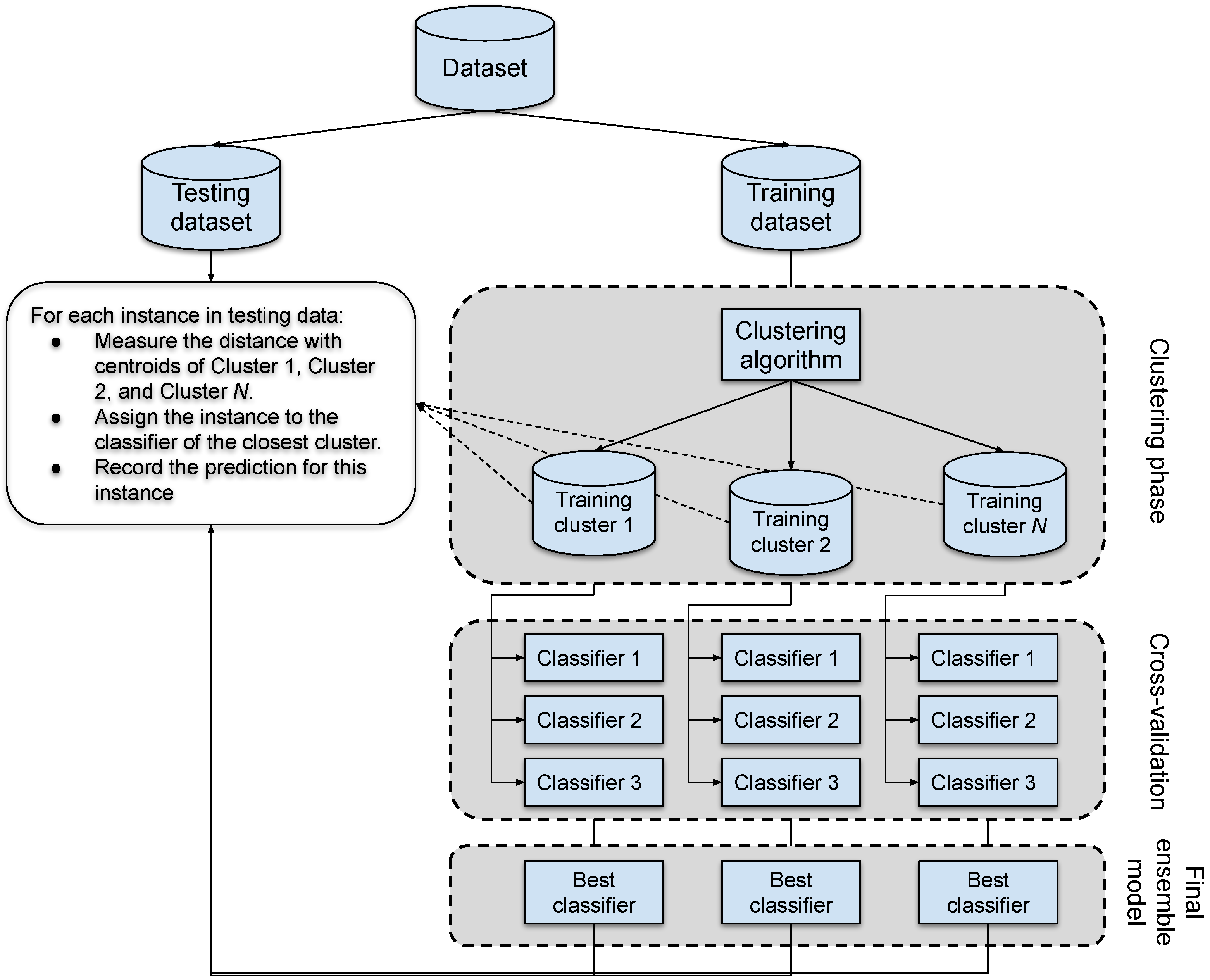
4. Proposed Approach
4.1. Clustering Phase
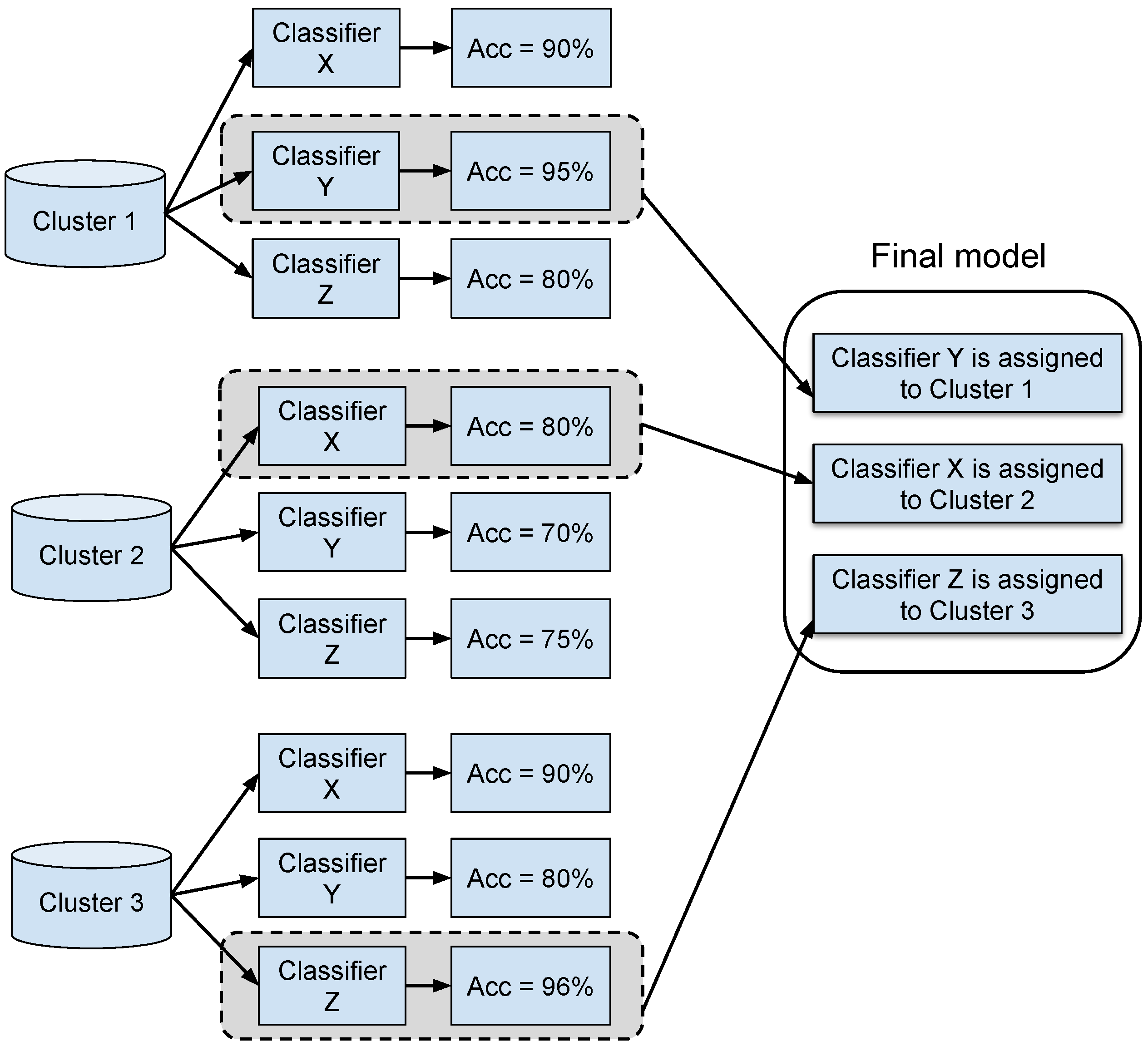
4.2. Models Development Phase
4.3. Testing Phase
| Algorithm 1: Ensemble with clustering. |
 |
5. Model Evaluation Metrics
- 1.
- Recall: is the fraction of relevant instances that have been retrieved over the total amount of relevant instances (i.e., coverage rate). It can be expressed by the following equation:
- 2.
- Precision: is the ratio of relevant instances among the retrieved instances. It can be given by the following equation:
- 3.
- G-mean: is the geometric mean of the recalls of each class and it can be measured by the following equation:
6. Datasets Description
7. Experiments and Results
- The best number of clusters is experimented for each dataset, and the best model for each cluster is found.
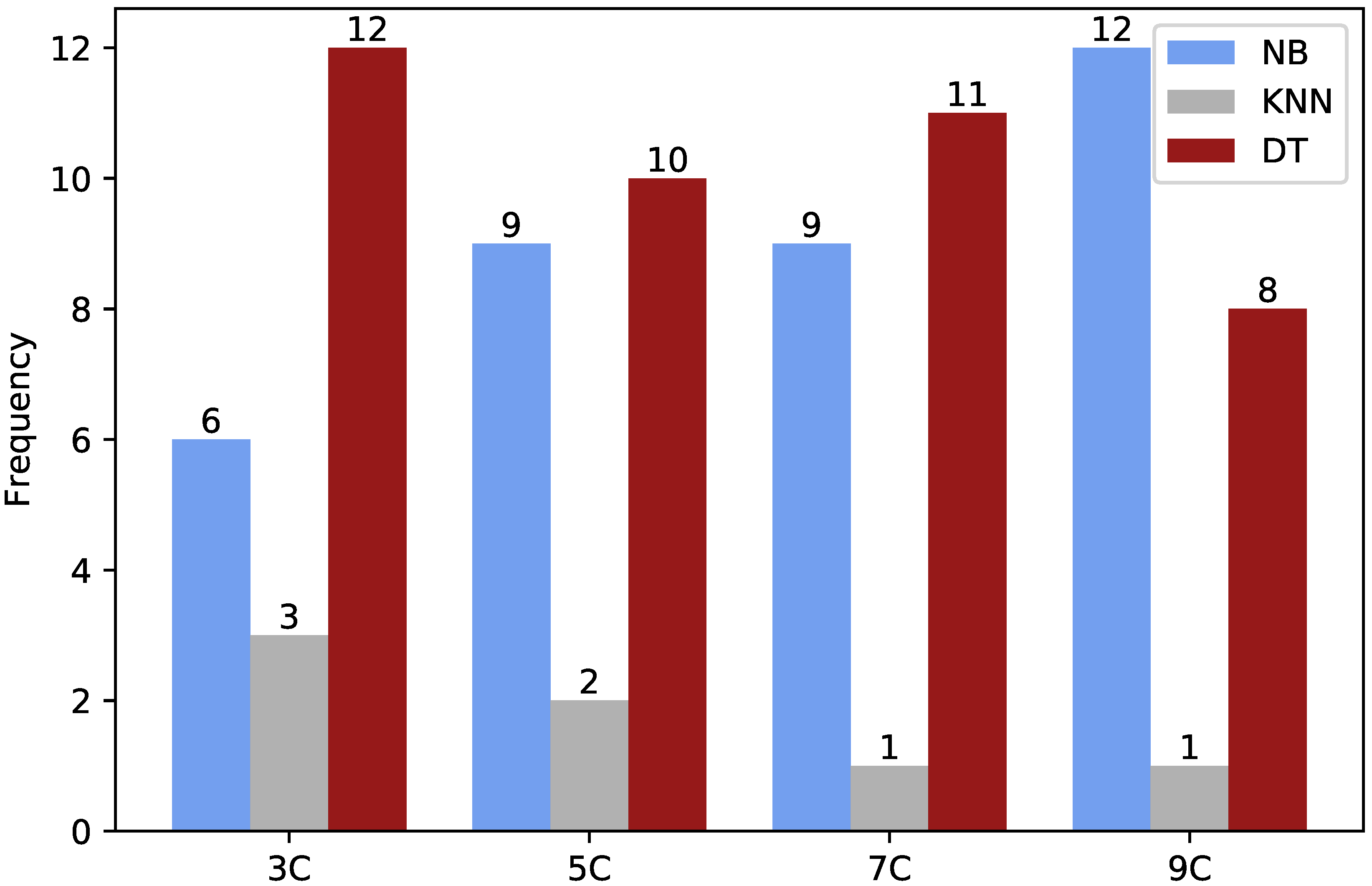
- The proposed approach is experimented based on utilizing simple and common classifiers (NB, k-NN, and DT).
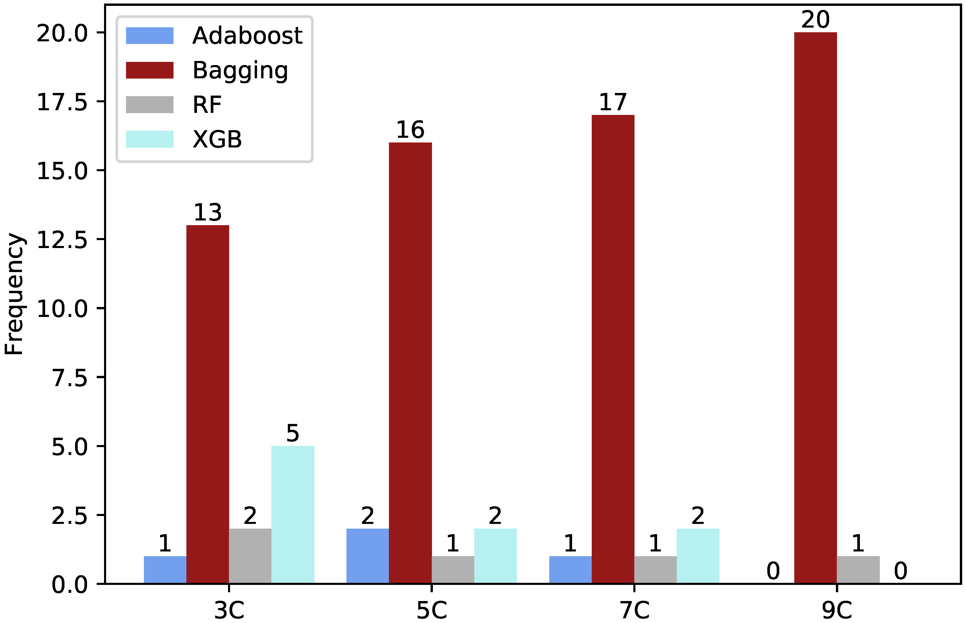
- The proposed approach is experimented based on utilizing powerful ensemble classifiers (Bagging, AdaBoost, RF, and XGB).
7.1. Finding the Best Number of Clusters and Their Corresponding Models
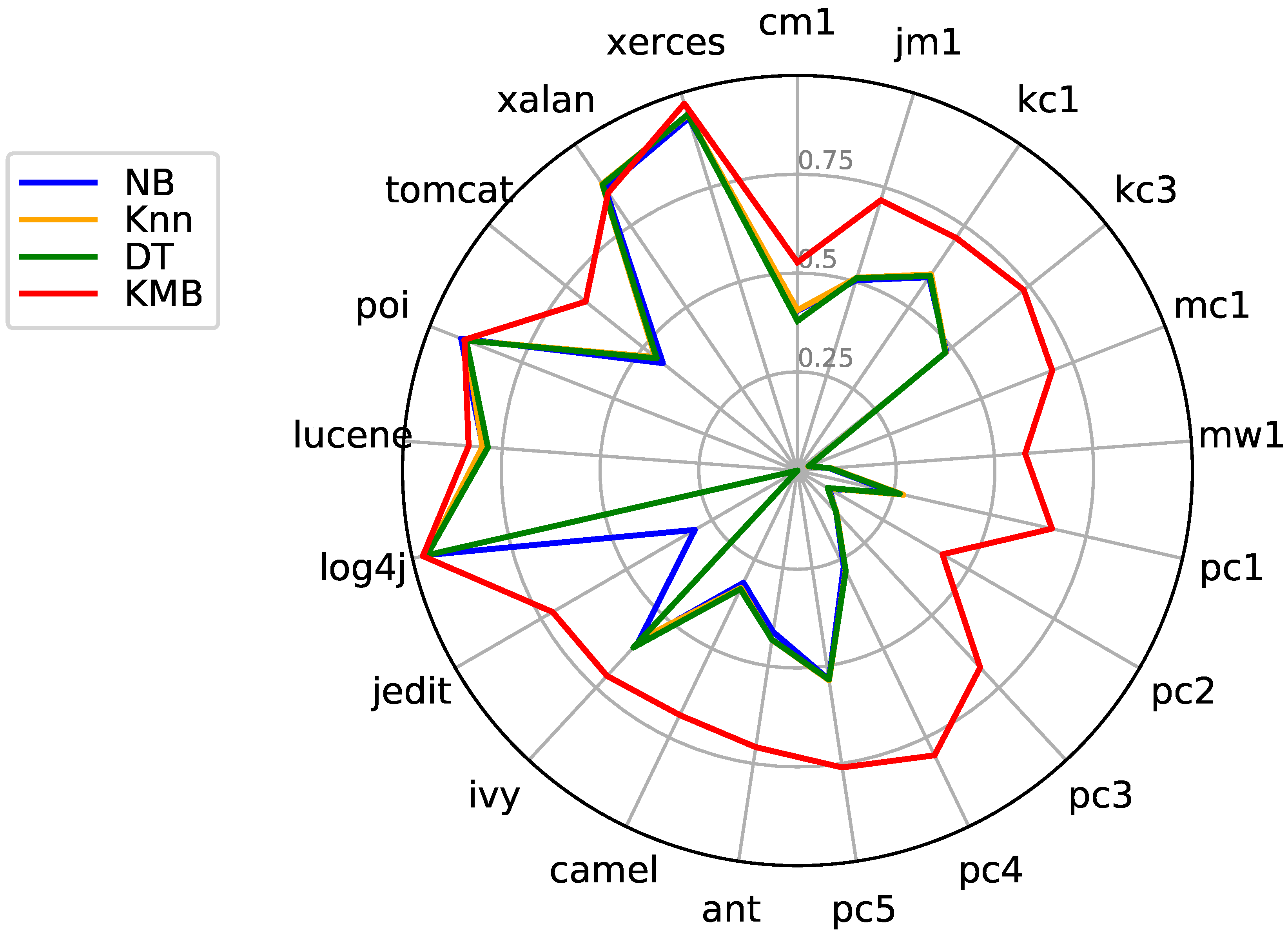
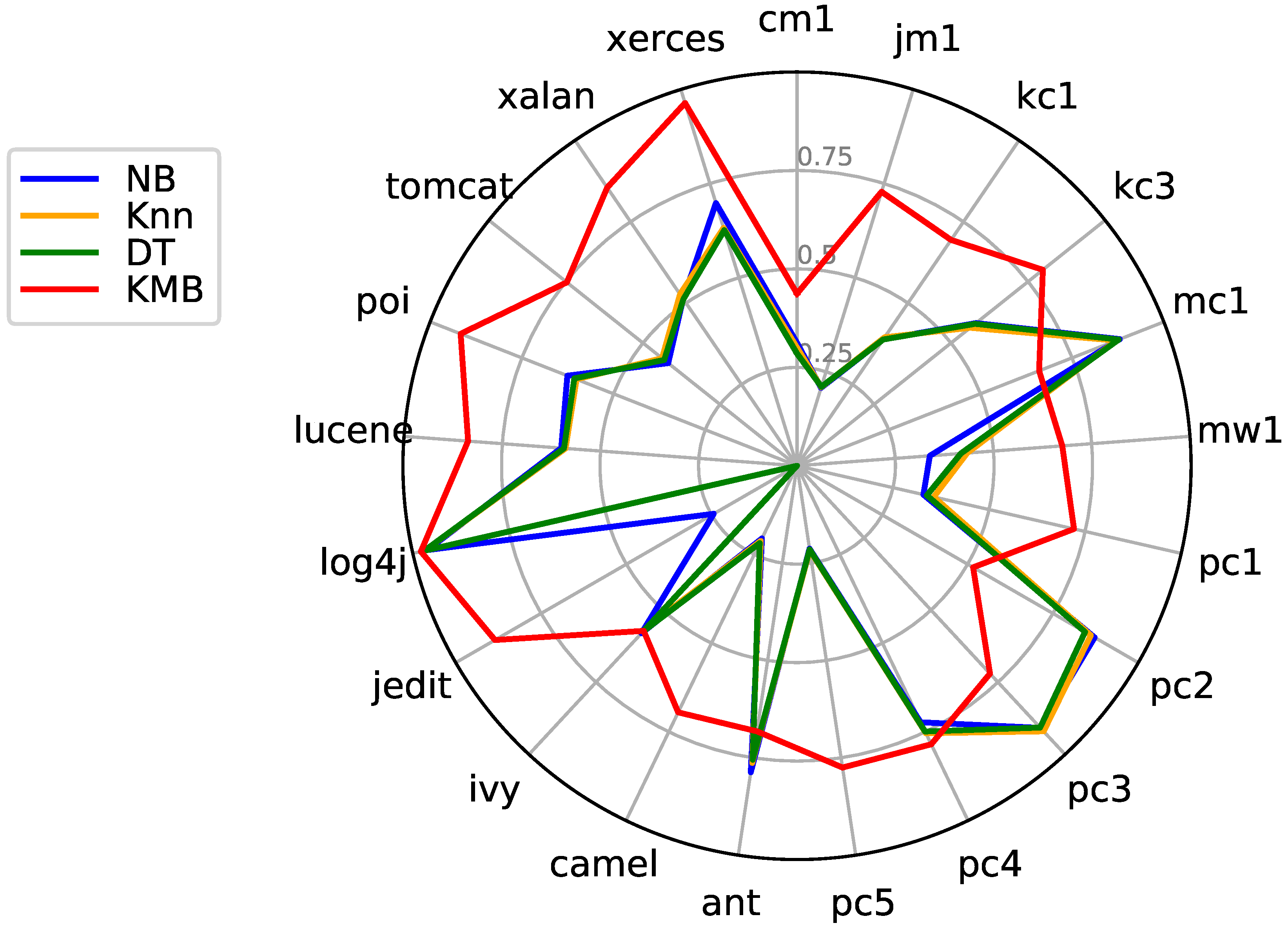
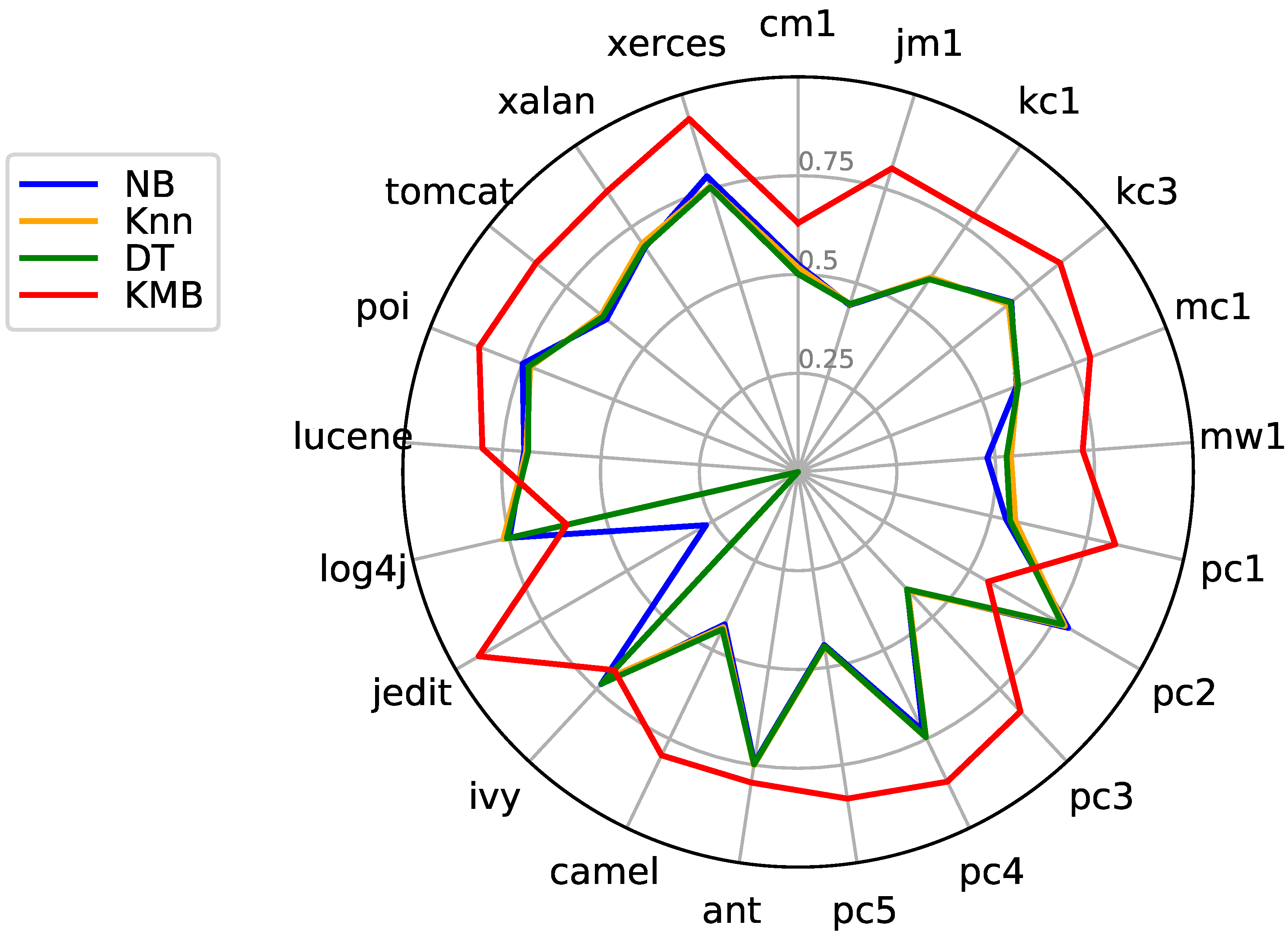
7.2. KMB vs. Basic Classifiers
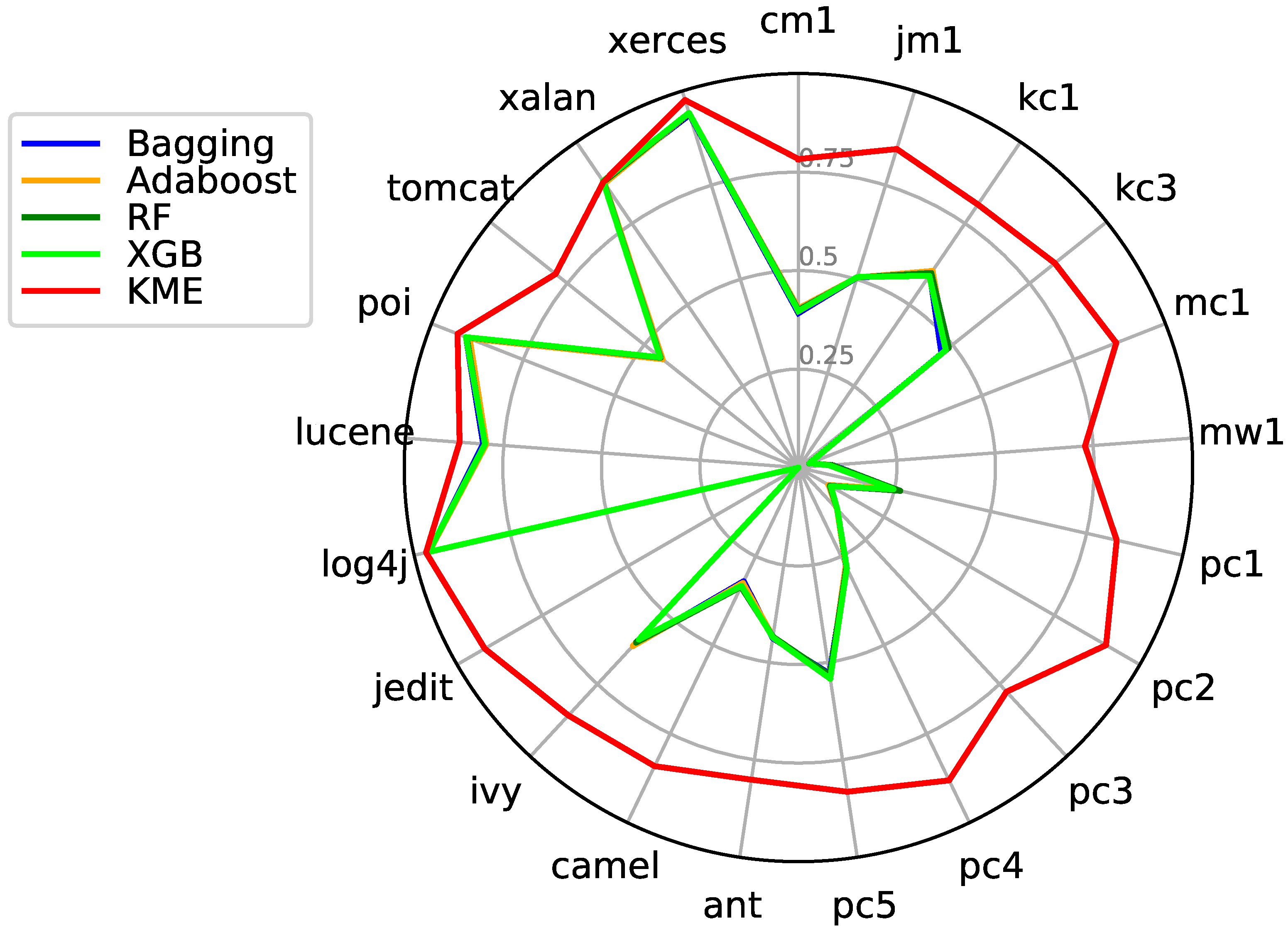
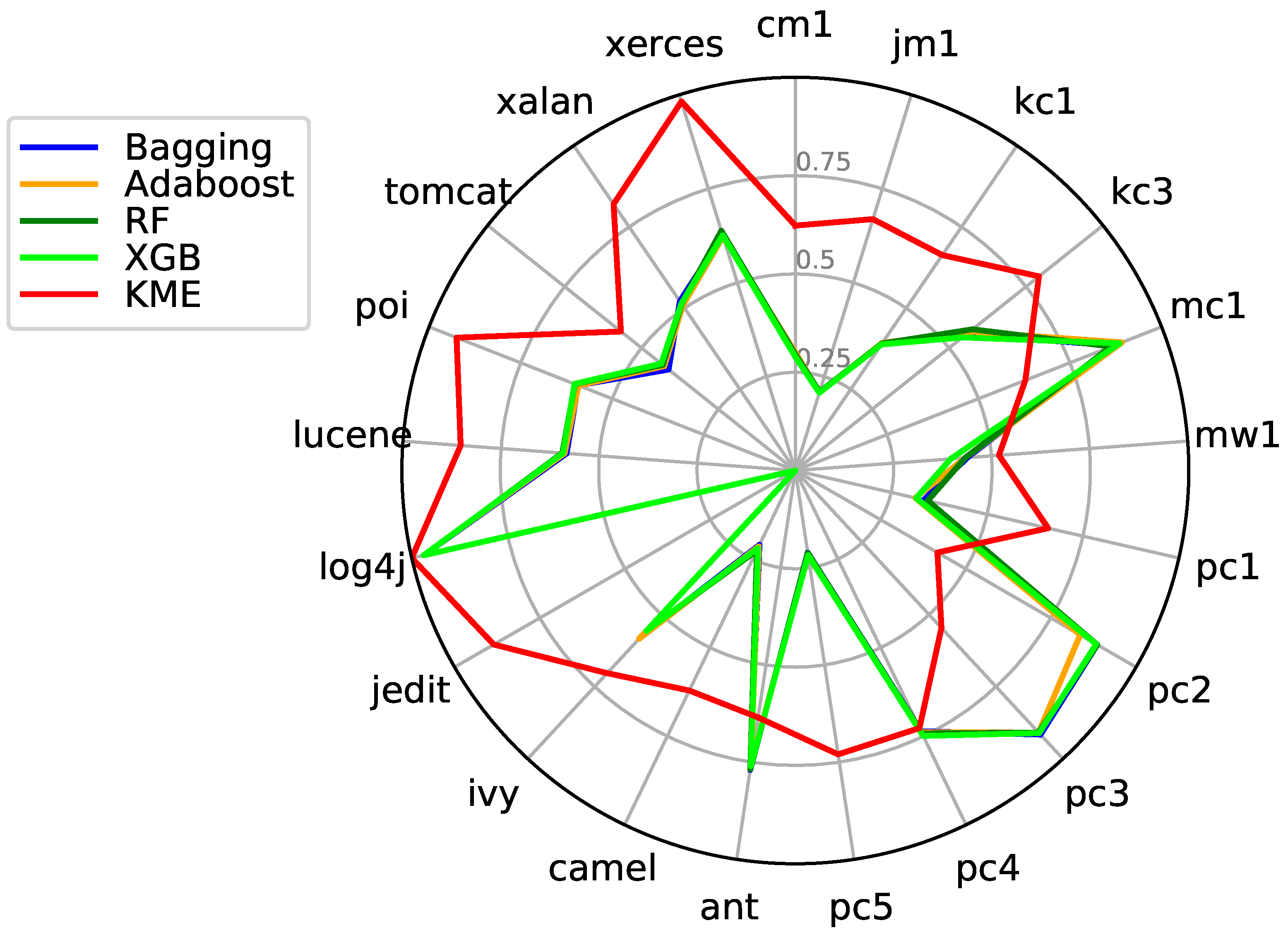
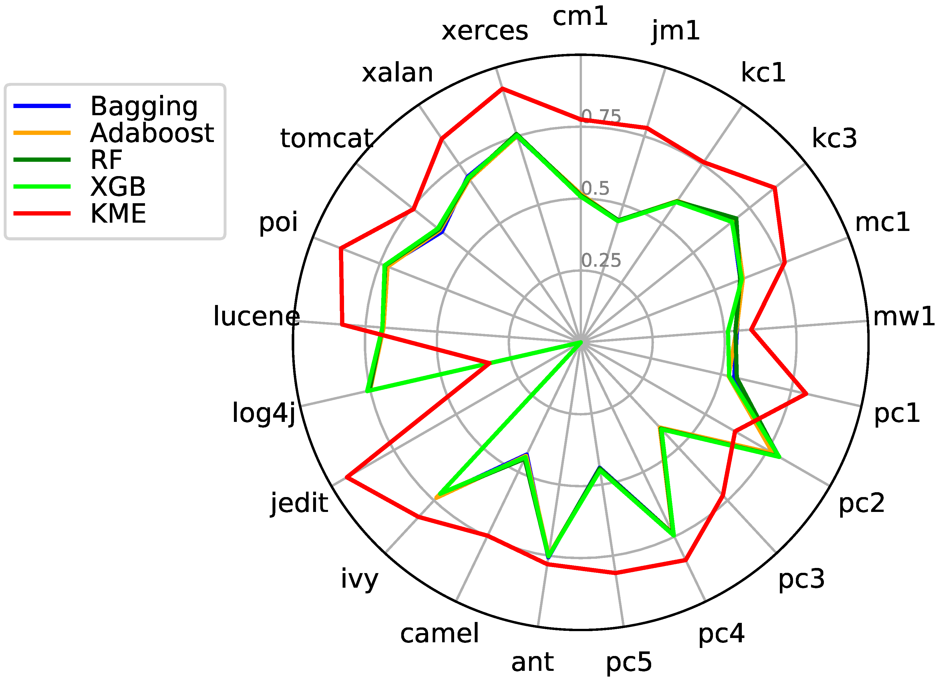
7.3. KME vs. Ensemble Classifiers
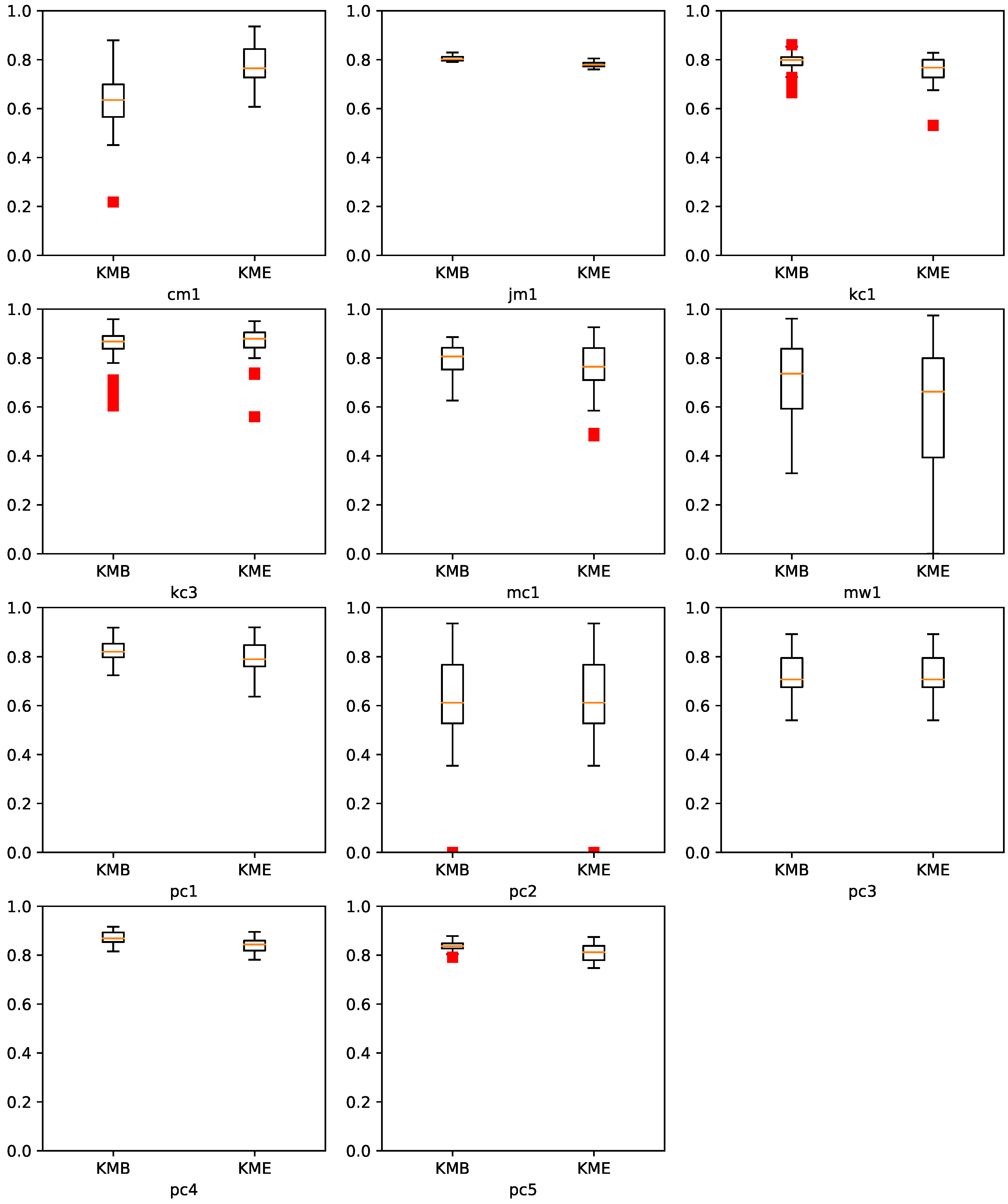
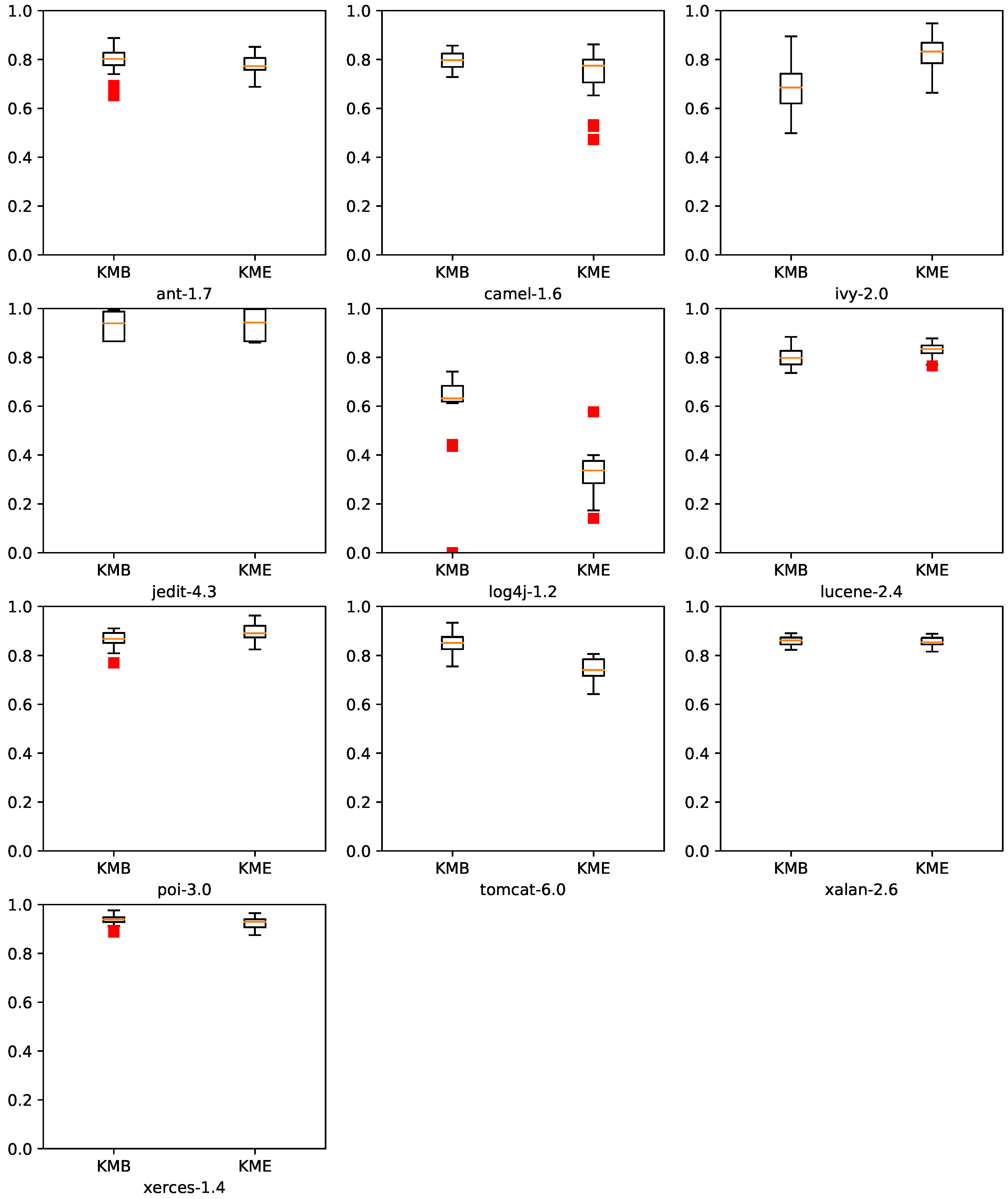
7.4. Statistical Test
8. Conclusions
Author Contributions
Funding
Conflicts of Interest
References
- Rawat, M.S.; Dubey, S.K. Software defect prediction models for quality improvement: A literature study. IJCSI Int. J. Comput. Sci. Issues 2012, 9, 288–296. [Google Scholar]
- Aljarah, I.; Banitaan, S.; Abufardeh, S.; Jin, W.; Salem, S. Selecting discriminating terms for bug assignment: A formal analysis. In Proceedings of the 7th International Conference on Predictive Models in Software Engineering, Banff, AB, Canada, 20–21 September 2011; p. 12. [Google Scholar]
- Fenton, N.E.; Neil, M. Software metrics: Roadmap. In Proceedings of the Conference on the Future of Software Engineering, Limerick, Ireland, 4–11 June 2000; pp. 357–370. [Google Scholar]
- Fenton, N.; Bieman, J. Software Metrics: A Rigorous and Practical Approach; CRC Press: Boca Raton, FL, USA, 2014. [Google Scholar]
- Moser, R.; Pedrycz, W.; Succi, G. A comparative analysis of the efficiency of change metrics and static code attributes for defect prediction. In Proceedings of the 2008 ACM/IEEE 30th International Conference on Software Engineering, Leipzig, Germany, 10–18 May 2008; pp. 181–190. [Google Scholar]
- Bhattacharya, P.; Iliofotou, M.; Neamtiu, I.; Faloutsos, M. Graph-based analysis and prediction for software evolution. In Proceedings of the 2012 34th International Conference on Software Engineering (ICSE), Zurich, Switzerland, 2–9 June 2012; pp. 419–429. [Google Scholar]
- Abaei, G.; Selamat, A. A survey on software fault detection based on different prediction approaches. Vietnam J. Comput. Sci. 2014, 1, 79–95. [Google Scholar] [CrossRef]
- Wang, S.; Liu, T.; Tan, L. Automatically learning semantic features for defect prediction. In Proceedings of the 38th International Conference on Software Engineering, Austin, TX, USA, 14–22 May 2016; pp. 297–308. [Google Scholar]
- Clark, B.; Zubrow, D. How Good Is the Software: A Review of Defect Prediction Techniques; Sponsored by the US Department of Defense; InSoftware Engineering Symposium, Carreige Mellon University: Pittsburgh, PA, USA, 2001. [Google Scholar]
- Hall, T.; Beecham, S.; Bowes, D.; Gray, D.; Counsell, S. A systematic literature review on fault prediction performance in software engineering. IEEE Trans. Softw. Eng. 2012, 38, 1276–1304. [Google Scholar] [CrossRef]
- Malhotra, R. A systematic review of machine learning techniques for software fault prediction. Appl. Soft Comput. 2015, 27, 504–518. [Google Scholar] [CrossRef]
- Menzies, T.; Milton, Z.; Turhan, B.; Cukic, B.; Jiang, Y.; Bener, A. Defect prediction from static code features: Current results, limitations, new approaches. Autom. Softw. Eng. 2010, 17, 375–407. [Google Scholar] [CrossRef]
- Li, Z.; Reformat, M. A practical method for the software fault-prediction. In Proceedings of the 2007 IEEE International Conference on Information Reuse and Integration, Las Vegas, IL, USA, 13–15 August 2007; pp. 659–666. [Google Scholar]
- Vandecruys, O.; Martens, D.; Baesens, B.; Mues, C.; De Backer, M.; Haesen, R. Mining software repositories for comprehensible software fault prediction models. J. Syst. Softw. 2008, 81, 823–839. [Google Scholar] [CrossRef]
- Mendes-Moreira, J.; Soares, C.; Jorge, A.M.; Sousa, J.F.D. Ensemble approaches for regression: A survey. ACM Comput. Surv. (CSUR) 2012, 45, 10. [Google Scholar] [CrossRef]
- Alsawalqah, H.; Faris, H.; Aljarah, I.; Alnemer, L.; Alhindawi, N. Hybrid SMOTE-Ensemble Approach for Software Defect Prediction. In Proceedings of the Computer Science On-Line Conference, Prague, Czech Republic, 26–29 April 2017; Springer: Cham, Switzerland, 2017; pp. 355–366. [Google Scholar]
- Rathore, S.S.; Kuamr, S. Comparative analysis of neural network and genetic programming for number of software faults prediction. In Proceedings of the 2015 National Conference on Recent Advances in Electronics & Computer Engineering (RAECE), Roorkee, India, 13–15 February 2015; pp. 328–332. [Google Scholar]
- Rathore, S.S.; Kumar, S. Predicting number of faults in software system using genetic programming. Procedia Comput. Sci. 2015, 62, 303–311. [Google Scholar] [CrossRef] [Green Version]
- Rathore, S.S.; Kumar, S. An empirical study of some software fault prediction techniques for the number of faults prediction. Soft Comput. 2016, 21, 7417–7434. [Google Scholar] [CrossRef]
- Rathore, S.S.; Kumar, S. Linear and non-linear heterogeneous ensemble methods to predict the number of faults in software systems. Knowl.-Based Syst. 2017, 119, 232–256. [Google Scholar] [CrossRef]
- Shatnawi, R.; Li, W. The effectiveness of software metrics in identifying error-prone classes in post-release software evolution process. J. Syst. Softw. 2008, 81, 1868–1882. [Google Scholar] [CrossRef]
- Sandhu, P.S.; Singh, S.; Budhija, N. Prediction of level of severity of faults in software systems using density based clustering. In Proceedings of the 2011 IEEE International Conference on Software and Computer Applications. IPCSIT, Kathmandu, Nepal, 1–2 July 2011. [Google Scholar]
- Menzies, T.; Greenwald, J.; Frank, A. Data mining static code attributes to learn defect predictors. IEEE Trans. Softw. Eng. 2007, 33, 2–13. [Google Scholar] [CrossRef]
- Suffian, M.D.M.; Ibrahim, S. A Prediction Model for System Testing Defects using Regression Analysis. arXiv 2014, arXiv:1401.5830. [Google Scholar]
- Koprinska, I.; Poon, J.; Clark, J.; Chan, J. Learning to classify e-mail. Inf. Sci. 2007, 177, 2167–2187. [Google Scholar] [CrossRef]
- Elish, K.O.; Elish, M.O. Predicting defect-prone software modules using support vector machines. J. Syst. Softw. 2008, 81, 649–660. [Google Scholar] [CrossRef]
- Huda, S.; Liu, K.; Abdelrazek, M.; Ibrahim, A.; Alyahya, S.; Al-Dossari, H.; Ahmad, S. An ensemble oversampling model for class imbalance problem in software defect prediction. IEEE Access 2018, 6, 24184–24195. [Google Scholar] [CrossRef]
- Jiang, Y.; Cukic, B.; Ma, Y. Techniques for evaluating fault prediction models. Empir. Softw. Eng. 2008, 13, 561–595. [Google Scholar] [CrossRef]
- Sun, Z.; Song, Q.; Zhu, X. Using coding-based ensemble learning to improve software defect prediction. IEEE Trans. Syst. Man Cybern. Part C (Appl. Rev.) 2012, 42, 1806–1817. [Google Scholar] [CrossRef]
- El Emam, K.; Benlarbi, S.; Goel, N.; Rai, S.N. Comparing case-based reasoning classifiers for predicting high risk software components. J. Syst. Softw. 2001, 55, 301–320. [Google Scholar] [CrossRef]
- Seliya, N.; Khoshgoftaar, T.M. Software quality estimation with limited fault data: A semi-supervised learning perspective. Softw. Qual. J. 2007, 15, 327–344. [Google Scholar] [CrossRef]
- Catal, C.; Sevim, U.; Diri, B. Software fault prediction of unlabeled program modules. In Proceedings of the World Congress on Engineering, London, UK, 1–3 July 2009; Volume 1, pp. 1–3. [Google Scholar]
- Yuan, X.; Khoshgoftaar, T.M.; Allen, E.B.; Ganesan, K. An application of fuzzy clustering to software quality prediction. In Proceedings of the 3rd IEEE Symposium on Application-Specific Systems and Software Engineering Technology, Richardson, TX, USA, 24–25 March 2000; pp. 85–90. [Google Scholar]
- Rathore, S.S.; Kumar, S. A study on software fault prediction techniques. Artif. Intell. Rev. 2019, 51, 255–327. [Google Scholar] [CrossRef]
- Challagulla, V.U.; Bastani, F.B.; Yen, I.L. A unified framework for defect data analysis using the mbr technique. In Proceedings of the 2006 18th IEEE International Conference on Tools with Artificial Intelligence (ICTAI’06), Arlington, VA, USA, 13–15 November 2006; pp. 39–46. [Google Scholar]
- Guo, L.; Cukic, B.; Singh, H. Predicting fault prone modules by the dempster-shafer belief networks. In Proceedings of the 18th IEEE International Conference on Automated Software Engineering, Montreal, QC, Canada, 6–10 October 2003; pp. 249–252. [Google Scholar]
- Catal, C. Software fault prediction: A literature review and current trends. Expert Syst. Appl. 2011, 38, 4626–4636. [Google Scholar] [CrossRef]
- Zhou, T.; Sun, X.; Xia, X.; Li, B.; Chen, X. Improving defect prediction with deep forest. Inf. Softw. Technol. 2019, 114, 204–216. [Google Scholar] [CrossRef]
- Quah, T.S.; Thwin, M.M. Application of neural networks for software quality prediction using object-oriented metrics. In Proceedings of the International Conference on Software Maintenance (ICSM 2003), Amsterdam, The Netherlands, 22–26 September 2003; pp. 116–125. [Google Scholar]
- Evett, M.; Khoshgoftar, T.; Chien, P.D.; Allen, E. GP-based software quality prediction. In Proceedings of the Third Annual Conference Genetic Programming, Madison, WI, USA, 22–25 July 1998; pp. 60–65. [Google Scholar]
- De Carvalho, A.B.; Pozo, A.; Vergilio, S.R. A symbolic fault-prediction model based on multiobjective particle swarm optimization. J. Syst. Softw. 2010, 83, 868–882. [Google Scholar] [CrossRef]
- Koru, A.G.; Liu, H. Building effective defect-prediction models in practice. IEEE Softw. 2005, 22, 23–29. [Google Scholar] [CrossRef]
- Qiu, S.; Lu, L.; Jiang, S.; Guo, Y. An investigation of imbalanced ensemble learning methods for cross-project defect prediction. Int. J. Pattern Recognit. Artif. Intell. 2019, 33, 1959037. [Google Scholar] [CrossRef]
- Peng, Y.; Kou, G.; Wang, G.; Wu, W.; Shi, Y. Ensemble of software defect predictors: An AHP-based evaluation method. Int. J. Inf. Technol. Decis. Mak. 2011, 10, 187–206. [Google Scholar] [CrossRef] [Green Version]
- Czibula, G.; Marian, Z.; Czibula, I. Software defect prediction using relational association rule mining. Inf. Sci. 2014, 264, 260–278. [Google Scholar] [CrossRef]
- Catal, C.; Diri, B. Software defect prediction using artificial immune recognition system. In Proceedings of the 25th conference on IASTED International Multi-Conference: Software Engineering, Innsbruck, Austria, 13–15 February 2007; pp. 285–290. [Google Scholar]
- Catal, C.; Diri, B. A fault prediction model with limited fault data to improve test process. In International Conference on Product Focused Software Process Improvement; Springer: Berlin/Heidelberg, Germany, 2008; pp. 244–257. [Google Scholar]
- Kanmani, S.; Uthariaraj, V.R.; Sankaranarayanan, V.; Thambidurai, P. Object-oriented software fault prediction using neural networks. Inf. Softw. Technol. 2007, 49, 483–492. [Google Scholar] [CrossRef]
- Begum, M.; Dohi, T. A Neuro-Based Software Fault Prediction with Box-Cox Power Transformation. J. Softw. Eng. Appl. 2017, 10, 288. [Google Scholar] [CrossRef] [Green Version]
- Köksal, G.; Batmaz, İ.; Testik, M.C. A review of data mining applications for quality improvement in manufacturing industry. Expert Syst. Appl. 2011, 38, 13448–13467. [Google Scholar] [CrossRef]
- Catal, C.; Sevim, U.; Diri, B. Practical development of an Eclipse-based software fault prediction tool using Naive Bayes algorithm. Expert Syst. Appl. 2011, 38, 2347–2353. [Google Scholar] [CrossRef]
- Son, L.H.; Pritam, N.; Khari, M.; Kumar, R.; Phuong, P.T.M.; Thong, P.H. Empirical Study of Software Defect Prediction: A Systematic Mapping. Symmetry 2019, 11, 212. [Google Scholar] [CrossRef] [Green Version]
- Challagulla, V.B.; Bastani, F.B.; Yen, I.L.; Paul, R.A. Empirical assessment of machine learning based software defect prediction techniques. Int. J. Artif. Intell. Tools 2008, 17, 389–400. [Google Scholar] [CrossRef]
- Catal, C.; Diri, B. Investigating the effect of dataset size, metrics sets, and feature selection techniques on software fault prediction problem. Inf. Sci. 2009, 179, 1040–1058. [Google Scholar] [CrossRef]
- Kaur, M.J.; Pallavi, M. Data mining techniques for software defect prediction. Int. J. Softw. Web Sci. (IJSWS) 2013, 3, 54–57. [Google Scholar]
- Kumar, M.A.; Gopal, M. Least squares twin support vector machines for pattern classification. Expert Syst. Appl. 2009, 36, 7535–7543. [Google Scholar] [CrossRef]
- Agarwal, S.; Tomar, D. A feature selection based model for software defect prediction. Assessment 2014, 65. [Google Scholar] [CrossRef]
- Tomar, D.; Agarwal, S. Prediction of defective software modules using class imbalance learning. Appl. Comput. Intell. Soft Comput. 2016, 2016, 6. [Google Scholar] [CrossRef] [Green Version]
- Shukla, H.; Verma, D.K. A Review on Software Defect Prediction. Int. J. Adv. Res. Comput. Eng. Technol. (IJARCET) 2015, 4, 4387–4394. [Google Scholar]
- Kumar Dwivedi, V.; Singh, M.K. Software Defect Prediction using Data Mining Classification Approach. Int. J. Technol. Res. Appl. 2016, 4, 31–35. [Google Scholar]
- Huda, S.; Alyahya, S.; Ali, M.M.; Ahmad, S.; Abawajy, J.; Al-Dossari, H.; Yearwood, J. A Framework for Software Defect Prediction and Metric Selection. IEEE Access 2018, 6, 2844–2858. [Google Scholar] [CrossRef]
- Bowes, D.; Hall, T.; Petrić, J. Software defect prediction: Do different classifiers find the same defects? Softw. Qual. J. 2018, 26, 525–552. [Google Scholar] [CrossRef] [Green Version]
- Turhan, B.; Bener, A.B. Software Defect Prediction: Heuristics for Weighted Naïve Bayes. In Proceedings of the ICSOFT (SE), Barcelona, Spain, 22–25 July 2007; pp. 244–249. [Google Scholar]
- Misirli, A.T.; Bener, A.B. A mapping study on bayesian networks for software quality prediction. In Proceedings of the 3rd International Workshop on Realizing Artificial Intelligence Synergies in Software Engineering, Hyderabad, India, 3 June 2014; pp. 7–11. [Google Scholar]
- Kotsiantis, S.B.; Zaharakis, I.; Pintelas, P. Supervised machine learning: A review of classification techniques. Emerg. Artif. Intell. Appl. Comput. Eng. 2007, 160, 3–24. [Google Scholar]
- Freund, Y.; Schapire, R.E. Experiments with a new boosting algorithm. Inicml 1996, 96, 148–156. [Google Scholar]
- Schapire, R.E. Explaining adaboost. In Empirical Inference; Springer: Berlin/Heidelberg, Germany, 2013; pp. 37–52. [Google Scholar]
- Freund, Y.; Schapire, R.E. A decision-theoretic generalization of on-line learning and an application to boosting. J. Comput. Syst. Sci. 1997, 55, 119–139. [Google Scholar] [CrossRef] [Green Version]
- Breiman, L. Bagging predictors. Mach. Learn. 1996, 24, 123–140. [Google Scholar] [CrossRef] [Green Version]
- Wang, T.; Li, W.; Shi, H.; Liu, Z. Software defect prediction based on classifiers ensemble. J. Inf. Comput. Sci. 2011, 8, 4241–4254. [Google Scholar]
- Breiman, L. Random forests. Mach. Learn. 2001, 45, 5–32. [Google Scholar] [CrossRef] [Green Version]
- Chen, T.; Guestrin, C. Xgboost: A scalable tree boosting system. In Proceedings of the 22nd ACM Sigkdd International Conference on Knowledge Discovery and Data Mining, San Francisco, CA, USA, 13–17 August 2016; pp. 785–794. [Google Scholar]
- Menzies, T.; Caglayan, B.; Kocaguneli, E.; Krall, J.; Peters, F.; Turhan, B. The Promise Repository of Empirical Software Engineering Data. Available online: http://promise.site.uottawa.ca/SERepositor (accessed on 1 April 2012).
- Shepperd, M.; Song, Q.; Sun, Z.; Mair, C. Data quality: Some comments on the nasa software defect datasets. IEEE Trans. Softw. Eng. 2013, 39, 1208–1215. [Google Scholar] [CrossRef] [Green Version]
- Ghotra, B.; McIntosh, S.; Hassan, A.E. Revisiting the impact of classification techniques on the performance of defect prediction models. In Proceedings of the 2015 IEEE/ACM 37th IEEE International Conference on Software Engineering, Florence, Italy, 16–24 May 2015; Volume 1, pp. 789–800. [Google Scholar]
- Lever, J.; Krzywinski, M.; Altman, N. Points of significance: Model selection and overfitting. Nat. Methods 2016, 13, 703–704. [Google Scholar] [CrossRef]


| Actual | ||
|---|---|---|
| Defect | No Defect | |
| Predicted defects | TP | FP |
| Predicted non-defects | FN | TN |
| Datasets | Attributes | Instances | Defects | Non-Defects | Defects% | Non-Defects % |
|---|---|---|---|---|---|---|
| cm1 | 38 | 327 | 42 | 285 | 12.8 | 87.2 |
| jm1 | 22 | 7782 | 1672 | 6110 | 21.5 | 78.5 |
| kc1 | 22 | 1183 | 314 | 869 | 26.5 | 73.5 |
| kc3 | 40 | 194 | 36 | 158 | 18.6 | 81.4 |
| mc1 | 39 | 1988 | 46 | 1942 | 2.3 | 97.7 |
| mw1 | 38 | 253 | 27 | 226 | 10.7 | 89.3 |
| pc1 | 38 | 705 | 61 | 644 | 8.7 | 91.3 |
| pc2 | 37 | 745 | 16 | 729 | 2.1 | 97.9 |
| pc3 | 38 | 1077 | 134 | 943 | 12.4 | 87.6 |
| pc4 | 38 | 1287 | 177 | 1110 | 13.8 | 86.2 |
| pc5 | 39 | 1711 | 471 | 1240 | 27.5 | 72.5 |
| ant-1.7 | 21 | 745 | 166 | 579 | 22.3 | 77.7 |
| camel-1.6 | 21 | 965 | 188 | 777 | 19.5 | 80.5 |
| ivy-2.0 | 21 | 352 | 40 | 312 | 11.4 | 88.6 |
| jedit-4.3 | 21 | 492 | 11 | 481 | 2.2 | 97.8 |
| log4j-1.2 | 21 | 205 | 189 | 16 | 92.2 | 7.8 |
| lucene-2.4 | 21 | 340 | 203 | 137 | 59.7 | 40.3 |
| poi-3.0 | 21 | 442 | 281 | 161 | 63.6 | 36.4 |
| tomcat-6 | 20 | 858 | 77 | 781 | 9 | 91 |
| xalan-2.6 | 21 | 885 | 411 | 474 | 46.4 | 53.6 |
| xerces-1.4 | 21 | 588 | 437 | 151 | 74.3 | 25.7 |
| Datasets | KMB | Best # of Clusters | Distribution of Classes Defects:Non-Defects | ||||
|---|---|---|---|---|---|---|---|
| 1C | 3C | 5C | 7C | 9C | |||
| cm1 | 0.518 | 0.608 | 0.723 | 0.744 | 0.845 | 9 | 7.7:92.3, 12.8:87.2, 14.3:85.7, 22.2:77.8, 50:50, 0:100, 0:100, 66.7:33.3, 13.8:86.2 |
| jm1 | 0.615 | 0.622 | 0.631 | 0.625 | 0.621 | 5 | 16.6:83.4, 23.2:76.8, 49.6:50.4, 12.2:87.8, 100:0 |
| kc1 | 0.628 | 0.594 | 0.722 | 0.625 | 0.592 | 5 | 17.8:82.2, 69.4:30.6, 50:50, 15:85, 44.2:55.8 |
| kc3 | 0.685 | 0.546 | 0.441 | 0.423 | 0.464 | 1 | 21.6:78.4 |
| mc1 | 0.385 | 0.559 | 0.340 | 0.680 | 0.716 | 9 | 5.6:94.4, 0:100, 3.5:96.5, 0:100, 2.6:97.4, 2:98, 0:100, 0:100, 50:50 |
| mw1 | 0.593 | 0.519 | 0.532 | 0.517 | 0.526 | 1 | 7.9:92.1 |
| pc1 | 0.556 | 0.603 | 0.548 | 0.414 | 0.453 | 3 | 13.5:86.5, 11.7:88.3, 2.3:97.7 |
| pc2 | 0.658 | 0.575 | 0.897 | 0.658 | 0.837 | 5 | 0:100, 0.8:99.2, 6.3:93.7, 0:100, 5.4:94.6 |
| pc3 | 0.633 | 0.549 | 0.565 | 0.534 | 0.538 | 1 | 11.9:88.1 |
| pc4 | 0.634 | 0.606 | 0.691 | 0.471 | 0.234 | 5 | 5.3:94.7, 5.8:94.2, 9.8:90.2, 12.1:87.9, 31.4:68.6 |
| pc5 | 0.671 | 0.641 | 0.617 | 0.653 | 0.559 | 1 | 26.1:73.9 |
| ant-1.7 | 0.574 | 0.460 | 0.427 | 0.486 | 0.639 | 9 | 2.8:97.2, 43.1:56.9, 5.8:94.2, 12.7:87.3, 86.7:13.3, 15:85, 16.7:83.3, 13.1:86.9, 40:60 |
| camel-1.6 | 0.619 | 0.588 | 0.611 | 0.540 | 0.562 | 1 | 17.3:65.4 |
| ivy-2.0 | 0.589 | 0.671 | 0.633 | 0.630 | 0.564 | 3 | 13.8:86.3, 5.6:94.4, 7.1:92.9 |
| jedit-4.3 | 0.826 | 0.458 | 0.458 | 0.633 | 0.650 | 1 | 0.8:99.2 |
| log4j-1.2 | 0.773 | 0.500 | 0.874 | 0.975 | 0.989 | 9 | 80:20, 93.1:6.9, 100:0, 87:13, 50:50, 100:0, 100:0, 100:0, 100:0 |
| lucene-2.4 | 0.734 | 0.822 | 0.720 | 0.592 | 0.548 | 3 | 51.9:48.1, 40.4:59.6, 67.8:32.2 |
| poi-3.0 | 0.817 | 0.653 | 0.526 | 0.551 | 0.567 | 1 | 60.2:39.8 |
| tomcat-6.0 | 0.640 | 0.666 | 0.726 | 0.346 | 0.513 | 5 | 37:63, 8.6:91.4, 2.3:97.7, 5.4:94.6, 9.6:90.4 |
| xalan-2.6 | 0.756 | 0.635 | 0.723 | 0.710 | 0.644 | 1 | 45.9:54.1 |
| xerces-1.4 | 0.843 | 0.864 | 0.843 | 0.886 | 0.759 | 7 | 89.3:10.7, 50:50, 92.1:7.9, 48.3:51.7, 90.5:9.5, 78.6:21.4, 100:0 |
| Datasets | KMB | Best # of Clusters | Distribution of Classes Defects: Non-Defects | ||||
|---|---|---|---|---|---|---|---|
| 1C | 3C | 5C | 7C | 9C | |||
| cm1 | 0.417 | 0.653 | 0.758 | 0.748 | 0.845 | 9 | 21.4:78.6, 5.9:94.1, 50:50, 0:100, 0:100, 41.7:58.3, 0:100, 13:87, 40:60 |
| jm1 | 0.505 | 0.585 | 0.596 | 0.612 | 0.606 | 7 | 19.7:80.3, 18.6:81.4, 50.6:49.4, 11.3:88.7, 100:0, 34.7:65.3, 68.2:31.8 |
| kc1 | 0.562 | 0.597 | 0.746 | 0.633 | 0.623 | 5 | 13.2:86.8, 42.9:57.1, 58.3:41.7, 26.2:73.8, 21.1:78.9 |
| kc3 | 0.759 | 0.569 | 0.481 | 0.447 | 0.491 | 1 | 25.8:74.2 |
| mc1 | 0.373 | 0.504 | 0.315 | 0.696 | 0.718 | 9 | 1.2:98.8, 1.6:98.4, 8.2:91.8, 0.9:99.1, 0:100, 0:100, 1.2:98.8, 13.6:86.4, 0:100 |
| mw1 | 0.661 | 0.526 | 0.539 | 0.522 | 0.524 | 1 | 8.7:91.3 |
| pc1 | 0.565 | 0.642 | 0.497 | 0.429 | 0.484 | 3 | 21.6:78.4, 11.2:88.8, 7.9:92.1 |
| pc2 | 0.402 | 0.484 | 0.913 | 0.672 | 0.840 | 5 | 0:100, 1.7:98.3, 2.3:97.7, 4.5:95.5, 16.7:83.3 |
| pc3 | 0.671 | 0.492 | 0.665 | 0.573 | 0.589 | 1 | 13.6:86.4 |
| pc4 | 0.695 | 0.664 | 0.697 | 0.503 | 0.229 | 5 | 10.1:89.9, 25.9:74.1, 2.6:97.4, 1:99, 19.6:80.4 |
| pc5 | 0.688 | 0.690 | 0.564 | 0.701 | 0.577 | 7 | 38.5:61.5, 21.8:78.2, 29.1:70.9, 36.7:63.3, 24.4:75.6, 72.7:27.3, 16.8:83.2 |
| ant-1.7 | 0.603 | 0.554 | 0.461 | 0.536 | 0.726 | 9 | 26.3:73.7, 35:65, 8.3:91.7, 11.9:88.1, 4.8:95.2, 10.3:89.7, 92.3:7.7, 57.1:42.9, 21.9:78.1 |
| camel-1.6 | 0.500 | 0.496 | 0.607 | 0.524 | 0.594 | 5 | 11.5:88.5, 20.1:79.9, 3.8:96.2, 27.6:72.4, 21.6:78.4 |
| ivy-2.0 | 0.657 | 0.861 | 0.719 | 0.681 | 0.636 | 3 | 15.4:84.6, 0:100, 18.7:81.3 |
| jedit-4.3 | 0.716 | 0.323 | 0.475 | 0.608 | 0.627 | 1 | 1.6:98.4 |
| log4j-1.2 | 0.667 | 0.472 | 0.890 | 0.977 | 0.987 | 9 | 91.7:8.3, 100:0, 100:0, 100:0, 100:0, 100:0, 100:0, 85.7:14.3, 90.5:9.5 |
| lucene-2.4 | 0.809 | 0.869 | 0.781 | 0.633 | 0.591 | 3 | 42.5:57.5, 66:34, 51.1:48.9 |
| poi-3.0 | 0.838 | 0.741 | 0.625 | 0.635 | 0.639 | 1 | 61.1:38.9 |
| tomcat-6.0 | 0.651 | 0.703 | 0.706 | 0.367 | 0.549 | 5 | 12.3:87.7, 5.1:94.9, 11.6:88.4, 0:100, 4.3:95.7 |
| xalan-2.6 | 0.793 | 0.736 | 0.774 | 0.767 | 0.727 | 1 | 46.2:53.8 |
| xerces-1.4 | 0.915 | 0.969 | 0.950 | 0.945 | 0.775 | 3 | 54.1:45.9, 93.2:6.8, 95.9:4.1 |
| Datasets | NB | k-NN | DT | KMB | ||||||||
|---|---|---|---|---|---|---|---|---|---|---|---|---|
| Pre | Rec | G-Mean | Pre | Rec | G-Mean | Pre | Rec | G-Mean | Pre | Rec | G-Mean | |
| cm1 | 0.404 | 0.312 | 0.525 | 0.406 | 0.300 | 0.517 | 0.379 | 0.285 | 0.501 | 0.527 | 0.437 | 0.630 |
| jm1 | 0.504 | 0.207 | 0.442 | 0.511 | 0.209 | 0.444 | 0.510 | 0.210 | 0.445 | 0.716 | 0.728 | 0.804 |
| kc1 | 0.592 | 0.389 | 0.591 | 0.601 | 0.395 | 0.596 | 0.596 | 0.388 | 0.590 | 0.713 | 0.694 | 0.787 |
| kc3 | 0.482 | 0.581 | 0.690 | 0.480 | 0.562 | 0.681 | 0.479 | 0.578 | 0.688 | 0.733 | 0.798 | 0.848 |
| mc1 | 0.029 | 0.880 | 0.594 | 0.029 | 0.870 | 0.596 | 0.030 | 0.877 | 0.598 | 0.693 | 0.660 | 0.794 |
| mw1 | 0.081 | 0.338 | 0.480 | 0.085 | 0.433 | 0.540 | 0.083 | 0.417 | 0.529 | 0.578 | 0.675 | 0.722 |
| pc1 | 0.250 | 0.329 | 0.540 | 0.275 | 0.356 | 0.564 | 0.266 | 0.338 | 0.550 | 0.661 | 0.721 | 0.823 |
| pc2 | 0.093 | 0.872 | 0.789 | 0.089 | 0.861 | 0.779 | 0.088 | 0.844 | 0.772 | 0.424 | 0.516 | 0.555 |
| pc3 | 0.144 | 0.908 | 0.406 | 0.146 | 0.920 | 0.409 | 0.144 | 0.907 | 0.405 | 0.680 | 0.720 | 0.827 |
| pc4 | 0.270 | 0.723 | 0.727 | 0.281 | 0.754 | 0.745 | 0.282 | 0.749 | 0.745 | 0.800 | 0.785 | 0.870 |
| pc5 | 0.535 | 0.213 | 0.443 | 0.537 | 0.217 | 0.448 | 0.535 | 0.215 | 0.446 | 0.760 | 0.775 | 0.836 |
| ant-1.7 | 0.413 | 0.787 | 0.745 | 0.433 | 0.763 | 0.751 | 0.433 | 0.755 | 0.748 | 0.708 | 0.682 | 0.795 |
| camel-1.6 | 0.315 | 0.205 | 0.428 | 0.330 | 0.212 | 0.436 | 0.333 | 0.218 | 0.442 | 0.687 | 0.695 | 0.796 |
| ivy-2.0 | 0.593 | 0.580 | 0.732 | 0.580 | 0.557 | 0.716 | 0.611 | 0.574 | 0.731 | 0.709 | 0.572 | 0.684 |
| jedit-4.3 | 0.300 | 0.244 | 0.269 | 0 | 0 | 0 | 0 | 0 | 0 | 0.716 | 0.885 | 0.933 |
| log4j-1.2 | 0.961 | 0.962 | 0.749 | 0.963 | 0.970 | 0.765 | 0.962 | 0.970 | 0.756 | 0.973 | 0.979 | 0.600 |
| lucene-2.4 | 0.799 | 0.600 | 0.695 | 0.800 | 0.589 | 0.690 | 0.786 | 0.593 | 0.685 | 0.835 | 0.837 | 0.801 |
| poi-3.0 | 0.915 | 0.626 | 0.749 | 0.902 | 0.601 | 0.728 | 0.901 | 0.607 | 0.732 | 0.906 | 0.917 | 0.867 |
| tomcat-6.0 | 0.436 | 0.418 | 0.620 | 0.461 | 0.438 | 0.637 | 0.456 | 0.431 | 0.631 | 0.686 | 0.747 | 0.848 |
| xalan-2.6 | 0.864 | 0.513 | 0.688 | 0.878 | 0.527 | 0.700 | 0.876 | 0.512 | 0.690 | 0.851 | 0.855 | 0.859 |
| xerces-1.4 | 0.934 | 0.698 | 0.783 | 0.942 | 0.632 | 0.756 | 0.943 | 0.626 | 0.754 | 0.972 | 0.964 | 0.935 |
| Datasets | Bagging | AdaBoost | RF | XGB | KME | ||||||||||
|---|---|---|---|---|---|---|---|---|---|---|---|---|---|---|---|
| Pre | Rec | G-Mean | Pre | Rec | G-Mean | Pre | Rec | G-Mean | Pre | Rec | G-Mean | Pre | Rec | G-Mean | |
| cm1 | 0.392 | 0.295 | 0.511 | 0.404 | 0.300 | 0.516 | 0.400 | 0.295 | 0.511 | 0.397 | 0.289 | 0.507 | 0.783 | 0.623 | 0.775 |
| jm1 | 0.505 | 0.207 | 0.441 | 0.505 | 0.208 | 0.443 | 0.505 | 0.209 | 0.444 | 0.506 | 0.207 | 0.441 | 0.846 | 0.669 | 0.780 |
| kc1 | 0.592 | 0.388 | 0.590 | 0.604 | 0.393 | 0.595 | 0.598 | 0.391 | 0.593 | 0.589 | 0.388 | 0.590 | 0.808 | 0.663 | 0.758 |
| kc3 | 0.464 | 0.556 | 0.674 | 0.480 | 0.567 | 0.684 | 0.488 | 0.576 | 0.691 | 0.478 | 0.543 | 0.672 | 0.832 | 0.792 | 0.862 |
| mc1 | 0.029 | 0.870 | 0.596 | 0.030 | 0.892 | 0.605 | 0.029 | 0.863 | 0.595 | 0.03 | 0.885 | 0.601 | 0.866 | 0.628 | 0.761 |
| mw1 | 0.087 | 0.438 | 0.544 | 0.086 | 0.433 | 0.542 | 0.085 | 0.433 | 0.539 | 0.078 | 0.396 | 0.513 | 0.729 | 0.519 | 0.594 |
| pc1 | 0.263 | 0.335 | 0.547 | 0.246 | 0.313 | 0.527 | 0.265 | 0.345 | 0.556 | 0.247 | 0.315 | 0.529 | 0.828 | 0.659 | 0.803 |
| pc2 | 0.094 | 0.886 | 0.795 | 0.088 | 0.836 | 0.771 | 0.092 | 0.886 | 0.792 | 0.095 | 0.883 | 0.796 | 0.901 | 0.417 | 0.619 |
| pc3 | 0.145 | 0.916 | 0.409 | 0.144 | 0.909 | 0.404 | 0.145 | 0.909 | 0.409 | 0.145 | 0.911 | 0.412 | 0.776 | 0.546 | 0.726 |
| pc4 | 0.280 | 0.736 | 0.739 | 0.276 | 0.739 | 0.738 | 0.280 | 0.742 | 0.741 | 0.283 | 0.749 | 0.745 | 0.881 | 0.727 | 0.840 |
| pc5 | 0.529 | 0.211 | 0.441 | 0.536 | 0.215 | 0.446 | 0.533 | 0.212 | 0.443 | 0.542 | 0.218 | 0.450 | 0.832 | 0.730 | 0.811 |
| ant-1.7 | 0.438 | 0.770 | 0.756 | 0.434 | 0.756 | 0.749 | 0.434 | 0.768 | 0.753 | 0.436 | 0.760 | 0.752 | 0.801 | 0.635 | 0.780 |
| camel-1.6 | 0.320 | 0.210 | 0.433 | 0.325 | 0.214 | 0.438 | 0.336 | 0.225 | 0.449 | 0.333 | 0.219 | 0.443 | 0.841 | 0.621 | 0.746 |
| ivy-2.0 | 0.616 | 0.569 | 0.728 | 0.618 | 0.584 | 0.737 | 0.606 | 0.553 | 0.717 | 0.595 | 0.556 | 0.718 | 0.858 | 0.703 | 0.828 |
| jedit-4.3 | 0 | 0 | 0 | 0 | 0 | 0 | 0 | 0 | 0 | 0 | 0 | 0 | 0.919 | 0.885 | 0.938 |
| log4j-1.2 | 0.961 | 0.969 | 0.752 | 0.961 | 0.969 | 0.751 | 0.962 | 0.967 | 0.753 | 0.962 | 0.969 | 0.761 | 0.969 | 1.000 | 0.325 |
| lucene-2.4 | 0.802 | 0.583 | 0.689 | 0.794 | 0.588 | 0.687 | 0.798 | 0.594 | 0.691 | 0.797 | 0.592 | 0.691 | 0.862 | 0.853 | 0.831 |
| poi-3.0 | 0.906 | 0.593 | 0.726 | 0.896 | 0.592 | 0.721 | 0.904 | 0.602 | 0.73 | 0.906 | 0.603 | 0.732 | 0.929 | 0.925 | 0.895 |
| tomcat-6.0 | 0.441 | 0.412 | 0.617 | 0.441 | 0.426 | 0.626 | 0.447 | 0.431 | 0.630 | 0.449 | 0.436 | 0.635 | 0.788 | 0.567 | 0.743 |
| xalan-2.6 | 0.879 | 0.521 | 0.697 | 0.873 | 0.508 | 0.687 | 0.877 | 0.513 | 0.691 | 0.880 | 0.514 | 0.693 | 0.878 | 0.820 | 0.857 |
| xerces-1.4 | 0.937 | 0.626 | 0.750 | 0.941 | 0.623 | 0.751 | 0.941 | 0.638 | 0.758 | 0.942 | 0.626 | 0.753 | 0.976 | 0.982 | 0.923 |
| Datasets | G-Mean | |
|---|---|---|
| KMB | KME | |
| cm1 | 0.630 | 0.775 |
| jm1 | 0.804 | 0.780 |
| kc1 | 0.787 | 0.758 |
| kc3 | 0.848 | 0.862 |
| mc1 | 0.794 | 0.761 |
| mw1 | 0.722 | 0.594 |
| pc1 | 0.823 | 0.803 |
| pc2 | 0.555 | 0.619 |
| pc3 | 0.827 | 0.726 |
| pc4 | 0.870 | 0.840 |
| pc5 | 0.836 | 0.811 |
| ant-1.7 | 0.795 | 0.780 |
| camel-1.6 | 0.796 | 0.746 |
| ivy-2.0 | 0.684 | 0.828 |
| jedit-4.3 | 0.933 | 0.938 |
| log4j-1.2 | 0.600 | 0.325 |
| lucene-2.4 | 0.801 | 0.831 |
| poi-3.0 | 0.867 | 0.895 |
| tomcat-6.0 | 0.848 | 0.743 |
| xalan-2.6 | 0.859 | 0.857 |
| xerces-1.4 | 0.935 | 0.923 |
| Datasets | Pre | Rec | ||
|---|---|---|---|---|
| DPDF | KME | DPDF | KME | |
| mc1 | 0.290 | 0.866 | 0.020 | 0.628 |
| mw1 | 0.630 | 0.729 | 0.430 | 0.519 |
| pc1 | 0.250 | 0.828 | 0.130 | 0.659 |
| pc2 | 0.980 | 0.901 | 0.720 | 0.417 |
| pc3 | 0.260 | 0.776 | 0.070 | 0.546 |
| pc4 | 0.770 | 0.881 | 0.210 | 0.727 |
| pc5 | 0.610 | 0.832 | 0.370 | 0.730 |
| ant-1.7 | 0.640 | 0.801 | 0.480 | 0.635 |
| camel-1.6 | 0.460 | 0.841 | 0.120 | 0.621 |
| lucene-2.4 | 0.690 | 0.862 | 0.820 | 0.853 |
| poi-3.0 | 0.840 | 0.929 | 0.820 | 0.925 |
| tomcat-6.0 | 0.840 | 0.788 | 0.120 | 0.567 |
| xalan-2.6 | 0.760 | 0.878 | 0.680 | 0.820 |
| Mean Rank (df = 8, N = 30) | |||||||||||
|---|---|---|---|---|---|---|---|---|---|---|---|
| KME | KMB | Ada | Bag | RF | XGB | NB | Knn | DT | Chi-Square | Asymp. Sig. | |
| cm1 | 8.870 | 7.000 | 4.700 | 4.000 | 4.130 | 3.850 | 4.450 | 4.330 | 3.670 | 98.860 | 0.000 |
| jm1 | 8.000 | 9.000 | 4.100 | 3.570 | 4.300 | 3.770 | 4.030 | 3.930 | 4.300 | 129.751 | 0.000 |
| kc1 | 8.100 | 8.670 | 4.130 | 3.530 | 4.000 | 3.900 | 4.080 | 4.650 | 3.930 | 121.136 | 0.000 |
| kc3 | 8.350 | 7.920 | 4.070 | 3.870 | 4.300 | 3.720 | 4.450 | 4.080 | 4.250 | 103.455 | 0.000 |
| mc1 | 7.933 | 8.433 | 4.650 | 3.850 | 3.767 | 4.517 | 3.783 | 4.033 | 4.033 | 107.854 | 0.000 |
| mw1 | 6.100 | 7.730 | 4.670 | 4.770 | 4.830 | 4.220 | 3.530 | 4.680 | 4.470 | 48.230 | 0.000 |
| pc1 | 8.430 | 8.570 | 3.380 | 4.270 | 4.350 | 3.320 | 3.920 | 4.600 | 4.170 | 132.182 | 0.000 |
| pc2 | 2.750 | 3.380 | 4.620 | 6.530 | 6.050 | 6.080 | 5.650 | 5.080 | 4.850 | 51.709 | 0.000 |
| pc3 | 8.100 | 8.900 | 3.650 | 4.250 | 3.880 | 4.550 | 3.730 | 4.120 | 3.820 | 129.866 | 0.000 |
| pc4 | 8.080 | 8.920 | 3.580 | 3.880 | 4.170 | 4.270 | 2.970 | 4.630 | 4.500 | 135.484 | 0.000 |
| pc5 | 8.200 | 8.800 | 3.870 | 3.730 | 3.630 | 4.230 | 3.830 | 4.570 | 4.130 | 129.298 | 0.000 |
| ant-1.7 | 6.630 | 7.530 | 4.270 | 4.970 | 4.700 | 4.420 | 3.720 | 4.320 | 4.450 | 49.926 | 0.000 |
| camel-1.6 | 8.200 | 8.767 | 4.080 | 3.630 | 4.850 | 4.250 | 3.220 | 3.800 | 4.200 | 132.108 | 0.000 |
| ivy-2.0 | 7.930 | 3.430 | 5.520 | 4.900 | 4.050 | 4.580 | 4.970 | 4.600 | 5.020 | 50.490 | 0.000 |
| jedit-4.3 | 8.630 | 8.130 | 3.850 | 3.850 | 3.850 | 3.850 | 5.130 | 3.850 | 3.850 | 213.087 | 0.000 |
| log4j-1.2 | 1.067 | 2.533 | 5.700 | 5.850 | 5.783 | 6.250 | 5.550 | 6.267 | 6.000 | 112.974 | 0.000 |
| lucene-2.4 | 8.730 | 8.230 | 3.800 | 3.920 | 3.930 | 4.120 | 4.420 | 4.230 | 3.620 | 127.274 | 0.000 |
| poi-3.0 | 8.700 | 8.300 | 3.200 | 3.480 | 3.930 | 4.000 | 5.280 | 3.850 | 4.250 | 137.046 | 0.000 |
| tomcat-6.0 | 7.700 | 9.000 | 3.630 | 3.650 | 3.880 | 4.520 | 3.900 | 4.500 | 4.220 | 122.274 | 0.000 |
| xalan-2.6 | 8.400 | 8.600 | 3.520 | 4.700 | 3.880 | 4.020 | 3.500 | 4.600 | 3.780 | 131.768 | 0.000 |
| xerces-1.4 | 8.370 | 8.630 | 3.030 | 3.580 | 3.970 | 3.470 | 6.430 | 3.850 | 3.670 | 155.979 | 0.000 |
© 2020 by the authors. Licensee MDPI, Basel, Switzerland. This article is an open access article distributed under the terms and conditions of the Creative Commons Attribution (CC BY) license (http://creativecommons.org/licenses/by/4.0/).
Share and Cite
Alsawalqah, H.; Hijazi, N.; Eshtay, M.; Faris, H.; Radaideh, A.A.; Aljarah, I.; Alshamaileh, Y. Software Defect Prediction Using Heterogeneous Ensemble Classification Based on Segmented Patterns. Appl. Sci. 2020, 10, 1745. https://doi.org/10.3390/app10051745
Alsawalqah H, Hijazi N, Eshtay M, Faris H, Radaideh AA, Aljarah I, Alshamaileh Y. Software Defect Prediction Using Heterogeneous Ensemble Classification Based on Segmented Patterns. Applied Sciences. 2020; 10(5):1745. https://doi.org/10.3390/app10051745
Chicago/Turabian StyleAlsawalqah, Hamad, Neveen Hijazi, Mohammed Eshtay, Hossam Faris, Ahmed Al Radaideh, Ibrahim Aljarah, and Yazan Alshamaileh. 2020. "Software Defect Prediction Using Heterogeneous Ensemble Classification Based on Segmented Patterns" Applied Sciences 10, no. 5: 1745. https://doi.org/10.3390/app10051745