Design Patterns for Resource-Constrained Automated Deep-Learning Methods
by
 , , , , , and
Lukas Tuggener
1,2,*,† ,
,
Mohammadreza Amirian
1,3,†,
Fernando Benites
1,
Pius von Däniken
1,
Prakhar Gupta
4,
Frank-Peter Schilling
1 and
Thilo Stadelmann
1,5
1
Institute of Applied Information Technology, School of Engineering, Zurich University of Applied Sciences ZHAW, 8400 Winterthur, Switzerland
2
Faculty of Informatics, Università della Svizzera italiana USI, 6900 Lugano, Switzerland
3
Institute of Neural Information Processing, Computer Science Department, Faculty of Engineering, Computer Science and Psychology, Ulm University, 89081 Ulm, Germany
4
Machine Learning and Optimization Laboratory, École Polytechnique Fédérale de Lausanne (EPFL), 1015 Lausanne, Switzerland
5
ECLT—European Centre for Living Technology, 30123 Venice, Italy
*
Author to whom correspondence should be addressed.
†
The authors contributed equally to this work.
AI 2020, 1(4), 510-538; https://doi.org/10.3390/ai1040031
Submission received: 18 September 2020
/
Revised: 28 October 2020
/
Accepted: 30 October 2020
/
Published: 6 November 2020
(This article belongs to the Section AI Systems: Theory and Applications)
Abstract
:We present an extensive evaluation of a wide variety of promising design patterns for automated deep-learning (AutoDL) methods, organized according to the problem categories of the 2019 AutoDL challenges, which set the task of optimizing both model accuracy and search efficiency under tight time and computing constraints. We propose structured empirical evaluations as the most promising avenue to obtain design principles for deep-learning systems due to the absence of strong theoretical support. From these evaluations, we distill relevant patterns which give rise to neural network design recommendations. In particular, we establish (a) that very wide fully connected layers learn meaningful features faster; we illustrate (b) how the lack of pretraining in audio processing can be compensated by architecture search; we show (c) that in text processing deep-learning-based methods only pull ahead of traditional methods for short text lengths with less than a thousand characters under tight resource limitations; and lastly we present (d) evidence that in very data- and computing-constrained settings, hyperparameter tuning of more traditional machine-learning methods outperforms deep-learning systems.
1. Introduction
Deep learning [1] has demonstrated outstanding performance for many tasks such as computer vision, audio analysis, natural language processing, or game playing [2,3,4,5], and across a wide variety of domains such as the medical, industrial, sports, and retail sectors [6,7,8,9]. However, the design, training, and deployment of high-performance deep-learning models requires human expert knowledge. Automated deep learning (AutoDL) [10] aims to provide deep models with the ability to be deployed automatically with no or significantly reduced human intervention. It achieves this through a combination of automated architecture search [11] with automated parameterization of the model as well as the training algorithm [12]. Its ultimate test is the use under heavy resource (i.e., time, memory, and computing) constraints. This is, from a scientific point of view, because only an AutoDL system that has attained a deeper semantic understanding of the task than is currently attainable can perform the necessary optimizations in a manner that is less brute-force and complies with the resource constraints [13]. From a practical point of view, operating under tight resource limitations is important as training deep architectures is already responsible for a worrying part of the world’s gross energy consumption [14,15], and only a few players could afford operating inefficient AutoDL systems on top of the many practical challenges involved [16,17].
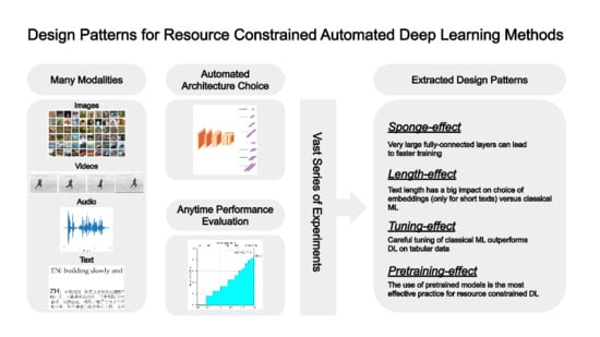
Many approaches exist that automate different aspects of a deep-learning systems (see Section 2), but there exists no general agreement upon the state of the art for fully automated deep learning. The AutoDL 2019 challenge series [18], organized by ChaLearn, Google, and 4paradigm, has to the best of our knowledge been the first effort to define such a state of the art [19]. AutoDL 2019 combines several successive challenges for different data modalities, including images and video, audio, text, and weakly supervised tabular data (see Figure 1). A particular focus is given to efficient systems under tight resource constraints. This is enforced by an evaluation metric that does not simply reward final model accuracy at the end of the training process, but rather the anytime performance, as measured by the integral of the learning curve as a function of logarithmically scaled training time (see Section 3). A good system thus must be as accurate as possible within the first seconds of training, and keep or increase this accuracy over time. This reflects practical requirements especially in mobile and edge computing settings [20].
The design of deep-learning models, by human experts or by an AutoDL system, would greatly benefit from an established theoretical foundation which is capable of describing relationships between model performance, model architecture and training data size [21]. In the absence of such a foundation [22], empirical relationships can be established which are able to serve as a guideline. This paradigm resulted in several recent empirical studies of network performance as a function of various design parameters [23,24,25], as well as novel, high-performing and efficient deep-learning architectures such as EfficientNet [26], RegNet [27] or DistilBERT [28].
In this paper, we systematically evaluate a wide variety of deep-learning models and strategies for efficient architecture design within the context of the AutoDL 2019 challenges. Our contribution is two-fold: first, we distill empirically confirmed behaviors in how different deep-learning models learn, based on a comprehensive survey and evaluation of known approaches; second, we formulate general design patterns out of the distilled behaviors on how to build methods with desirable characteristics in settings comparable to the AutoDL challenges, and highlight especially promising directions for future investigations. In particular, our most important findings are:
- Sponge effect: very large fully connected layers can learn meaningful audio and image features faster. → Resulting design pattern: make the classifier part in the architecture considerably larger than suggested by current best practices and fight overfitting, leading to higher anytime performance.
- Length effect: word embeddings play out their strength only for short texts in the order of hundreds of characters under strict time and computer source constraints. → Resulting design pattern: for longer texts in the order of thousands of characters, use traditional machine learning (ML) techniques such as Support Vector Machines and hybrid approaches, leading to higher performance faster.
- Tuning effect: despite recent trends in the literature, deep-learning approaches are out-performed by carefully tuned traditional ML methods on weakly supervised tabular data. → Resulting design pattern: in data-constrained settings, avoid overparameterization and consider traditional ML algorithms and extensive hyperparameter search.
- Pretraining-effect: leveraging pretrained models is the single most effective practice in confronting computing resources constraints for AutoDL. → Resulting design pattern: prefer fine-tuning of pretrained models over architecture search where pretrained models on large datasets are available.
The overall target of these design patterns is high predictive performance, fast training speed and high out-of-the-box generalization performance for unseen data. The remainder of this work is organized as follows: Section 2 surveys the most important related work. Section 3 introduces the general goals and performance metrics used, before we follow the structure of the sub-challenges of the AutoDL 2019 competition and derive design patterns and directions per modality in Section 4, Section 5, Section 6 and Section 7, based on a thorough evaluation of a broad range of approaches. Section 8 then consolidates our findings from the individual modalities and discusses overarching issues concerning all aspects of architecture design for AutoDL. Finally, in Section 9, we offer conclusions on the presented design choices for AutoDL, highlighting major open issues.
2. Survey of Related Work
Automated machine learning (AutoML) and by extension AutoDL is usually defined as the combined algorithm selection and hyperparameter optimization (CASH) problem [29], which encompasses choice and parameterization of both a machine-learning model and a respective training algorithm—all without any human input. In the following, we give an overview of those AutoDL aspects with highest relevancy to this work.
2.1. Hyperparameter Optimization
The performance of machine-learning and especially deep-learning methods crucially depend well-chosen hyperparameters. The task of optimizing these manually is often laborious or even impossible. Hyperparameter optimization (HPO) [12] research tackles this sub-task of AutoML. Among its most important challenges are (a) the computational expensiveness of evaluating many sets of hyperparameter combinations on a given deep-learning architecture, (b) the high dimensionality and complexity of the search space (including co-dependencies among different hyperparameters), and (c) the lack of information on the shape of the loss surface as well as its gradients with respect to the hyperparameters. Therefore, the HPO problem is typically tackled using general purpose black box optimization techniques:
Common model free black box optimization methods are grid search [30] and random search [31]. In grid search, a range of viable values are chosen per hyperparameter and the model is evaluated for the Cartesian product over all the choices made. Due to scaling exponentially with respect to search space dimensionality and polynomially with respect to grid resolution, an exhaustive grid search is often prohibitively computationally costly. Alternatively, in random search, randomly sampled configurations of hyperparameters are evaluated until a certain budget of computational resources is exhausted. It can also be used in conjunction with local search [32]. Genetic or evolutionary algorithms [33] operate on an evolving population of candidate solutions. Both can be parallelized in a straightforward way [34], and have been applied successfully in deep learning [35].
Bayesian optimization [36] is a powerful framework for optimizing expensive black box functions. The main idea is to model the response surface of the black box using a probabilistic surrogate model described as Gaussian processes [37] or estimated by random forests [38] and the Tree Parzen Estimator [39]. The second core component is the acquisition function, which uses the surface prediction of the surrogate model to decide where to sample the next point of the black box, therefore balancing exploration versus exploitation. The concept of using the true loss in combination with early stopping as a surrogate loss can be taken even further by combining early stopping with learning curve predictions, leading to predictive termination [40]. The fact that there is currently no large difference in performance between random search and more sophisticated methods testifies to the difficulty of the HPO problem [41].
2.2. Neural Architecture Search
Neural architecture search (NAS), which is concerned with automatically finding high-performing neural network architectures, can be categorized along three dimensions [11]:
The search space encompasses all possible model architectures that can be theoretically found using a specific NAS method. However, a search space constrained by prior knowledge might lead to the NAS system not finding an optimal architecture that looks very different from human crafted architectures. A common search space definition is an arbitrary length chain of known operations such as convolution, pooling, or fully connected layers, together with their respective hyperparameters (number of filters, kernel size, activation function etc.) [42]. Limiting the search space to the design of a characteristic block or cell that is then stacked, e.g., the inception module [43], leads to a much reduced search space and thus accelerated search [44].
Common search strategies build on HPO methods and include random search as a strong baseline [45], as well as Bayesian optimization, gradient-based methods, evolutionary strategies, or reinforcement learning (RL). The literature is inconclusive whether the latter two consistently outperform random search [46].
Performance estimation of an architecture under consideration using the standard method of employing training and validation datasets usually leads to a huge, often prohibitive, demand for computational resources. Therefore, NAS often relies on cheaper but less accurate surrogate metrics such as validation of models trained with early stopping [10], on lower-resolution input [47], or with fewer filters [46]. In the context of AutoML, NAS can be employed in two ways: offline, in conjunction with a performance measure that emphasizes generalizability to a new task, or online, to directly find an architecture that is tuned to the task at hand.
2.3. Meta-Learning
Meta-learning [48] comprises methods to gather and analyze relevant data on how machine-learning methods performed in the past (meta-data) to inform the future design and parameterization of machine-learning algorithms (“learning how to learn”). A rich source of such meta-data are the metrics of past training runs, such as learning curves or time until training completion [49]. By statistically analyzing a meta-data database of sufficient size it is possible to create a sensitivity analysis that shows which hyperparameters have a high influence on performance [50]. This information can be leveraged to significantly improve HPO by restricting the search space to parameters of high importance.
A second important source of meta-data are task-specific summary statistics called meta-features, designed to characterize task datasets [51]. Examples for such statistics are the number of instances in a dataset or a class distribution estimate. There are many other commonly used meta-features mostly based on statistics or information theory. An extended overview is available in Vanschoren [48]. A more sophisticated approach is to learn, rather than manually define, meta-features [52,53].
As there is no free lunch [54], it is important to make sure that the meta-data used originates from use cases that carry at least some resemblance to the target task. The closer the use cases from which the meta-data is constructed, and the target task are in distribution, the more effective meta-learning becomes. When the similarity is strong enough (e.g., different computer vision tasks on real world photos), it is helpful to not only inform the algorithm choice and parameterization by meta-learning but also the model weights by using transfer learning [55].
Instead of initializing the model weights from scratch, transfer learning [55] suggests re-using weights from a model that has been trained for a general task on one or multiple large datasets. In a second step, the weights are only fine-tuned on the data for the task at hand. The use of such pretrained models [56] has been applied extensively and successfully e.g., for vision [57] and natural language processing tasks [58], although the opposite effect, longer training and lower prediction quality, is also possible if tasks or datasets are not compatible [59]. Transfer learning can be taken even further by training models with a modified loss that increases transferability, such as MAML [60].
2.4. Empirical Guidelines for Designing Neural Networks
In the light of the aforementioned difficulties to ground design choices in the absence of an overarching theory [61], there has been a trend of using vast empirical studies to distill guidelines on designing neural networks. Several such studies recently established relationships between model performance and various design parameters. The effect of data size on the generalization error in vision, text, and speech tasks was studied and a strikingly consistent power-law behavior was observed in a large set of experiments [23], extended by a recent study of the dependence of the generalization error on both data size and model size for a variety of datasets [24]. In a recent survey, the effect of model size, data size and training time on performance was systematically studied in the context of language models, yielding several empirical scaling laws [25].
EfficientNet [26] is a good example of translating such observations into novel deep-learning model architectures that are at the same time high-performing and resource efficient. Here, it was observed that scaling width, depth, and input resolution has combined positive effects larger than scaling each factor in isolation. More recently, a study aimed at finding neural network design spaces with a high density of good models (RegNet) [27]. This study revealed that having roughly 20 convolutional blocks is a good number across many different network scales (mobile settings up to big networks). The most successful network architectures in the given search space also effectively ignored bottleneck, reverse bottleneck, as well as depth-wise convolutions, which is surprising since all these paradigms are very prevalent in contemporary neural network design best practices.
3. Study Design
In the remainder of this paper, the findings of our systematic evaluation of AutoDL strategies are presented, structured according to the following data modalities: visual, audio, text, and tabular data, based on the sub-challenges of the AutoDL competition. Each modality is presented in a distinct section, each following the same structure (see Figure 2). Each section discusses the search for a suitable model, its evaluation and interim conclusions for a given data modality. The work is reproducible by using our code which has been published on GitHub [62], it is conveniently usable in conjunction with the starting kit provided by the challenge organizers [63].
The quantitative metrics for this study are motivated by the goal of deriving general design patterns for automated deep-learning methods specifically for heavily resource-constrained settings. This study is conducted within the environment of the AutoDL 2019 competition. In accordance with the competition rules, developed models are evaluated with respect to two quantitative metrics: final predictive performance as well as sample and resource efficiency [19]. Final model accuracy thereby is captured by the Normalized Area Under the ROC Curve (NAUC). In the binary classification setting, this corresponds to where AUC is the well-known Area Under the Receiver Operating Characteristic curve. In the multi-class case the AUC is computed per class and averaged. Resource efficiency is measured by the Area Under the Learning Curve (ALC), which takes training speed and hence training sample efficiency into account. Another term for this used throughout this paper is anytime performance.
Learning curves, as depicted in Figure 3, plot the predictive performance in terms of NAUC versus logarithmically transformed and normalized time which is defined in the AutoDL 2019 competition as follows [19]:
Here, T is the available time budget, t is the elapsed time in seconds and is a constant used for scaling and normalization. Time and performance are both normalized to 1 and the area under the learning curve (ALC), computed using the trapezoidal rule, is a normalized measure between 0 and 1. Figure 3 illustrates the workings of NAUC and ALC by means of two models and their performance. The first model shows higher predictive performance at the end; however, it trains significantly slower and therefore demonstrates lower anytime performance. The logarithmic scaling of the time axis emphasizes the early training stages for the computation of ALC.
4. Methods for Visual Data
Our evaluation of AutoDL strategies for visual data in this section is performed in the context of the AutoCV2 sub-challenge of the 2019 AutoDL challenges, which fully contains AutoCV1.
4.1. Background
The goal of the AutoCV2 sub-challenge is the development of a system that is able to perform multi-label and multi-class classification of images and videos of any type without human intervention. Seven datasets are available for offline model development and training (for details see Table 1). Developed models can then be validated on five unknown datasets (two containing images, three containing videos). The final evaluation is performed on five private datasets.
Based on the results of our evaluation we establish specific patterns for designing successful vision systems with respect to the metrics defined in Section 3. As a baseline model we adopt MobileNetV2 [64], inspired by the runner-up of AutoCV1 [65]. Initial tests showed that pretraining on ImageNet [66] is absolutely necessary, therefore all subsequent experiments are conducted using pretrained models.
4.2. Base Architecture Selection
The basic neural network architecture is a crucial choice for any deep-learning system. This is especially true for automated deep learning where next to predictive performance, flexibility is very important. The recently introduced EfficientNets [26] are a strong candidate architecture (see Section 2.4) as they combine top performance with lean design. The most appealing feature of the EfficientNet in the context of AutoDL is that the architecture incorporates two natural scaling parameters, which can be used to scale the base network up (wider and deeper) or down (shallower and narrower). To test our hypothesis that EfficientNet is a solid choice in an AutoDL setting, we benchmark the smallest configuration used in the original publication, EfficientNet-B0 (scaling: ), as well as an even smaller version we call EfficientNet-mini (scaling: ), against our baseline of MobileNetV2 (using otherwise similar hyperparameters). On top of each model, a classifier consisting of two fully connected layers of size 512 and no regularization is used.
The benchmark results in Table 2 show that EfficientNet-B0 has high predictive performance as indicated by the NAUC score. In terms of ALC, the much smaller and faster MobileNetV2 scores highest for each dataset. EfficientNet-mini is not a worthwhile compromise, since it is only marginally faster than EfficientNet-B0 while having a considerably worse predictive performance. These results lead to the verdict that in a time-sensitive setting MobileNetV2 is preferred, while under less tight time constraints or for more complicated vision tasks EfficientNet-B0 definitely is a good choice. For strong anytime performance, it is recommended to use a combination of both architectures and select the more appropriate model based on the availability of data and complexity of the image classification task.
4.3. Classifier Design
Apart from the base architecture, the size and design of the fully connected classifier layers are the most important design choices when building a Convolutional Neural Network (CNN). The first question that needs to be answered is how the extracted features are fed into the classifier. Two common options are to reshape the output to have dimension one in height and width (flatten), or to compute the average over height and width (spatial pooling). For videos, there is the additional time dimension which can be pooled (temporal pooling). Experiments on all datasets (see Table 3) conclusively show that spatial pooling is the best option.
The second important characteristic is the number of layers and number of neurons per layer of the fully connected classifier. We tested different one- and two-layer classifiers from 64 neurons in a single layer up to two times 1024 neurons in two layers. Figure 4 shows a very interesting phenomenon: big classifiers are able to absorb information faster and therefore learn much quicker during the first couple of iterations. We dubbed this the sponge effect, as the fast information intake resembles a sponge being immersed in water. The sponge effect can be exploited whenever a network design needs to be adapted for fast training speeds. As we observe that this phenomenon is not only relevant to vision, we will present a more detailed, multi-modal, investigation in Section 5.6.
4.4. Globally Suitable Hyperparameter Settings
Even a well-designed network architecture can completely fail when the wrong hyperparameters are chosen. Section 2 introduced existing methods for finding suitable hyperparameters, but these methods are too slow to be used in an online fashion when optimizing for an anytime-performance metric such as ALC. Hence, online HPO is not possible and it is mandatory to find good default values that generalize well to as many scenarios as possible. This is achieved by studying different hyperparameter choices on the offline training datasets.
Figure 5 shows the results of a grid search for weight decay and learning rate of the AdamW optimizer [67]. In the case of learning rate, it shows very clearly that a value of performs well for every dataset. For weight decay, the agreement among the datasets is much lower and the result is therefore harder to interpret. When the performance is averaged over all datasets, we obtain a maximum performance point for weight decay that is not strictly optimal for any of the datasets, but performs well on all of them.
4.5. Integrating the Time Dimension of Videos
Video data differs from image data by having an additional dimension: time. There exist different approaches for processing this additional dimension, from 3D CNNs [68] that naturally incorporate a third dimension, to temporal pooling which simply averages over time. 3D convolutions have a very heavy memory and computing consumption. The lightweight 2+1-dimensional (2+1D) architecture for action recognition in videos, proposed in Ref. [69], is based on a modified ResNet-18 architecture [70], where after each residual block a one-dimensional convolution in the temporal direction is inserted. This allows the network to learn temporal and spatial structures independently with a very light model, at the disadvantage of not being able to learn interactions between the temporal and spatial information.
Table 4 shows that the 2+1D model exhibits poor performance in terms of ALC. To speed the model up, we made it even more lightweight by removing all but the last two temporal convolutions (2+1D small), which yields a significant performance boost. The last architecture we evaluate is based on the MobileNetV2 baseline. We use a single three-dimensional convolution in place of temporal pooling (Late 3D). This approach yields by far the best results.
4.6. Interim Conclusions
Our evaluations yield observations that may help optimizing a vision system for AutoDL in an anytime-performance-oriented setting. Making models smaller makes them faster and therefore suited for fast learning. We could show that for certain hyperparameters (e.g., learning rate, pooling), a relatively simple evaluation can conclusively reveal the best choice for a resource-constrained setting. We also established that having a large classifier increases training speed through better sample efficiency. This rather counter-intuitive sponge effect can lead to bigger models training faster than smaller ones and is further discussed in Section 5.6.
5. Methods for Audio Data
This section describes the unique challenges and opportunities in automated audio processing in the context of the AutoSpeech challenge of AutoDL 2019 and presents empirical results. The model search space covers preprocessing, model development, architecture search, and building ensembles. We compare the proposed architectures, present principles for model design and give research directions for future work.
5.1. Background
Although training an ensemble of classifiers for automated computer vision is not possible in a resource-constrained environment, this limitation does not exist for audio data due to the much smaller dataset and model sizes. Lightweight architectures pretrained and optimized on ImageNet [2] are common choices for computer vision tasks. However, in the case of audio classification, such pretrained and optimized architectures are not yet abundant, though starting points exist: AudioSet [71], a dataset of over 5000 h of audio with 537 classes, as well as the VoxCeleb speaker recognition datasets [72,73], aim at providing an equivalent of ImageNet for audio and speech processing. Researchers trained computer vision models, such as VGG16, ResNet-34 and ResNet-50, on these large audio datasets to develop generic models for audio processing [73,74]. However, architecture search and established bases for transfer learning for audio processing remain an open research topic.
The AutoSpeech challenge spans a wide range of speech and music classification tasks (for details see Table 5). The small size of the development datasets provides the chance of developing ensembles even under tight time and computing constraints; nonetheless poses the challenge of overfitting and the general problem of finding good hyperparameter settings for preprocessing. The five development datasets from AutoSpeech are used to optimize and evaluate the proposed models for automated speech processing. The audio sampling rate for all datasets is 16 KHz, and all the tasks are about multi-class classification. The available computing resources are one NVIDIA Tesla P100 GPU, a 4-core CPU, 26 GB of RAM, and the time is limited to 30 min.
5.2. Preprocessing
Both raw audio, in the form of time series data, and preprocessed audio converted to a 2D time-frequency representation, provide the necessary information for pattern recognition. The standard for preprocessing and feature extraction in the case of speech data is to compute the Mel-spectrogram [75] and then derive the Mel-Frequency Cepstral Coefficients (MFCCs) [76]. The main challenge of this preprocessing is the high number of related hyperparameters. Table 6 presents three candidate sets of hyperparameters for automated audio processing: the default hyperparameters of the LibROSA Python library [77], hyperparameters from the first attempt on using deep learning for speaker clustering [78], and our empirically optimized hyperparameters derived for the AutoSpeech datasets There is no single choice of hyperparameters which outperforms the others for all datasets. Therefore, optimizing the preprocessing for specific tasks or datasets based on trainable preprocessing is a potential subject for future research.
5.3. Modeling
One-dimensional CNNs and Recurrent Neural Networks (RNNs) such as Long Short-Term Memory (LSTM) cells [79] or Gated Recurrent Units (GRUs) [80,81] are the prime candidates for processing raw audio signals as time series. Two-dimensional RNNs and CNNs can process preprocessed audio in the form of Mel-spectrograms and MFCCs.
Table 7 presents a performance comparison for three architectures. The first model uses MFCC features and applies GRUs to them for classification. The second model is a four-layer CNN with global max-pooling and a fully connected layer on top. This model is the result of a grid search on kernel size, number of filters, and size of the fully connected layers. The third model is an 11-layer CNN for audio embedding extraction called VGGish [74], pretrained on an audio dataset that is part of the Youtube-8m dataset [82]. Here, it is worth mentioning that training on raw audio using LSTMs or GRUs requires more time, which is at odds with our goal to train the best model under limited time and computing resources. The results presented in Table 7 support the idea that the model produced by architecture search performs better than the other models in terms of accuracy and sample efficiency. The simple CNN model outperforms the rest in terms of NAUC and ALC, except for accent classification, while VGGish profits from pretraining on additional data in language classification.
The models in Table 7 have enough capacity to memorize the entire development datasets for all tasks. Therefore, the pressing issue here is preventing overfitting and optimizing the generalizability of the models to unseen data. Reducing overfitting in small data settings is easier with the smaller CNN model compared to a larger model such as VGGish. Another way to tackle this issue is to develop augmentation strategies. SpecAugment [83] represents one of the first approaches towards augmentation for audio data. The principle of manual augmentation design can be extended to automated augmentation policy search. Investigating possible audio augmentation policies manually or automatically, similar to AutoAugment [84] for image processing, is a promising direction for future studies.
5.4. Ensembles
Given the provided computing resources, size of datasets and model complexity, it is possible to train an ensemble of classifiers. Such models can be trained either in parallel or sequentially. The sequential approach trains the models one after another and the final prediction is computed by averaging the probability estimates of all models. The parallel approach trains a set of models simultaneously and combines the predictions through trainable output weights. Sequential training shows better performance at the beginning of the training by concentrating on smaller models and training them first, optimizing anytime performance. On the other hand, the parallel approach divides the computing resources among all models and optimizes the combination of the predictions: by optimizing the weights of the ensemble members via gradient descent, it naturally focuses on pushing smaller models with earlier predictive performance at the beginning of the training process, and shifts that focus towards the more complex hence better final performing models towards the end. Table 8 presents the results obtained using both types of ensembles. Both approaches show merit although no approach is superior on all datasets.
5.5. Interim Conclusions
Finding the optimal preprocessing for audio classification is challenging due to the large number of hyperparameters. There is not a single set of hyperparameters which outperforms all others for all audio classification tasks. Therefore, a trainable preprocessing unit to adjust the hyperparameters to a given dataset is an exciting possibility for future research. Our experimental results demonstrate that architecture search is the most fruitful direction in model design to achieve optimal performance for small datasets. Furthermore, there is an opportunity to develop more lightweight pretrained architectures specifically for audio processing using the AudioSet and VoxCeleb datasets, similar to what is available to the computer vision community with ImageNet-pretrained models. The results confirm that building an ensemble of models is an efficient way to improve the final performance in the studied setting. Nevertheless, most of the applied methods suffer from overfitting. Establishing best practices for automated augmentation thus represents a final promising line of future studies.
5.6. The Sponge Effect in Vision and Audio Processing
As discussed in Section 4, Figure 4 reveals the interesting phenomenon we dubbed sponge effect that large fully connected classifiers initially learn much faster than small ones. In this section, we study this effect more closely for the modalities of vision and audio. We do this by fitting our models with different classifiers—small to large, one, and two layers—on all datasets available for both modalities. Since the datasets and models are much smaller for audio than for vision, we use 16, 32, 64 and 128 neurons per layer for audio and 64, 256, 512 and 1024 neurons per layer for vision, respectively.
We test for the sponge effect by investigating the performance for the two first evaluations of each model, occurring after 10 and 35 minibatches of size 25 for vision, and after 5 and 11 training epochs for audio. We average the performance over the first two evaluations, as well as over all available datasets. The results are presented in Figure 6, using MobileNetV2 for vision and the average of the 4-layer CNN and VGGish for audio. It clearly shows that the sponge effect is present in the vision and audio models.
Even though the sponge effect is very apparent in the first training stage, the classifier size correlates much less with the final performance of a model. This observation demonstrates that increasing the classifier predictability (size) is not a free win, but there is a trade-off between training speed and proneness of a model to overfitting. Hence, the combination of large classifiers with sample-efficient regularization techniques, such as fast AutoAugment [85] or early stopping, is a promising step forward.
6. Methods for Textual Data
In this section, we report on our findings with respect to natural language processing tasks as evaluated in the AutoNLP sub-challenge of AutoDL 2019.
6.1. Background
The natural language processing (NLP) challenge is about classifying text samples in a multi-class setting for a variety of datasets. We evaluate standard machine learning versus a selection of deep-learning approaches: the successful deep word embeddings [86], a standard approach for text classification, Term-Frequency-Inverse-Document-Frequency (TF-IDF, [87]), for feature extraction and weighting (vectorization) and Support Vector Machines (SVM) [88] with linear kernels as classifiers. This can compete in many cases with the state of the art [89], especially for small datasets. Additionally, it is difficult to develop features as good as TF-IDF, which has a global view of the data, when processing a few samples sequentially.
Deep-learning methods can be developed on patterns mined from large corpora by using methods such as said word embeddings [86] as well as Transformers, e.g., BERT [58], achieving highest prediction quality in text classification tasks. A key aspect to consider when choosing a method to use—as we will see later—is the characteristics of the dataset, implying the length effect.
The data for AutoNLP encompasses 16 datasets with texts in English (EN) and Chinese (ZH). We concentrate on the evaluation on the 6 offline datasets that involve a broad spectrum of classification subject domains (see Table 9). The distribution of samples per class is mostly balanced. Dataset O3 is a notable exception, showing severe class imbalance of 1 negative example for roughly every 500 positive ones. The English datasets have about 3 Million tokens from which 243,515 are unique words (a relatively large vocabulary). The Chinese datasets have 52,879,963 characters with 6641 of them being unique (A comparison is difficult since “这是鸟” means “this is a bird” whereas “工业化” means “industrialization” (from [90])). Since the ALC metric is also used in this competition, producing fast predictions is imperative. Preprocessing is a key component to optimize, especially since some texts are quite long.
6.2. Preprocessing
The first step is to select a tokenizer for the specific languages. After tokenization, the texts are vectorized, meaning words are converted to indices and their occurrences counted. We increased the number of extracted features over time, as we will describe later.
Language dependency: The preprocessing is language dependent, specifically using a different tokenizer, and in part removing stop words in English. The chosen tokenizer for English is a regex-based word tokenizer [91], whereas for Chinese a white-space aware character-wise tokenizer (char_wb) or the Jieba tokenizer is chosen [92].
Vectorization: A traditional word count vectorizer needs to build up and maintain an internal dictionary for checking word identities and mapping them to indices. We instead apply the hashing trick [93] which has several advantages. It removes the need for an internal dictionary by instead applying a hash function to every input token to determine its index. It can therefore be applied in an online fashion without precomputing the whole vocabulary and is trivially parallelizable, which is crucial in a time-constrained setting. We weight the Hashing Vectorizer counts (term frequency) with inverse document frequency (TF-IDF).
N-gram features: Simple unigram feature extraction is the fastest method, but cannot grasp the dependency between words. We therefore increase the width of n-grams, i.e., the number of neighboring tokens we group together for counting, in each iteration and change the tokenization from words to characters and back depending on the number of n-grams. Using multiple word and character n-grams proved to be successful [89] in other NLP competitions. Naively using n-grams, without applying lemmatization or handling synonyms, might produce lower prediction quality, but these more advanced methods need much more time to preprocess than is available in the resource-constrained settings.
Online TF-IDF: IDF weights are usually computed over the whole training corpus. We apply a modified version that can be trained on partial data and is updated incrementally.
Word embeddings: For each language fastText embeddings [94] were available in the competition, i.e., for each word a dense representation in a 300-dimensional space is provided. Even though these embeddings were developed for deep learning they can also be used as features for a SVM by summing the individual embeddings of each word per sample (e.g., sentence) [95].
6.3. Classifiers
In the following section we present our baseline and improved classifiers as well as the three best ranked approaches from the competition (The three highest-ranked participants were requested to publish their code after the competition):
CNN: We used a simple 2 layer stacked CNN as a baseline for deep-learning methods. Each layer of the CNN has a convolutional layer, max-pooling, dropout () and 64 filters. The classifier consists of 3 dense layers (128, 128 and 60 neurons). We choose CNNs because they train much faster and require less data than RNNs or Transformers.
BERT: Since the Huggingface transformers library [96] was allowed in the competition, we perform the classification with some of its models, namely BERT [58] and distilled BERT [28]. We report here only the results using BERT, since it achieves higher final NAUC, whereas distilled BERT has higher ALC. The reason of choosing NAUC over ALC is that we are interested in assessing how much better an unconstrained complex language model can perform compared to our other approaches.
SVM: Unlike deep-learning methods, SVMs with linear kernels converge to a solution very quickly. We focus on feature extraction when designing different solutions since brute-force tuning of hyperparameters is prone to overfitting to certain datasets. In particular, we evaluate the following SVM-based approaches:
- SVM 1-GRAM: A simple combination of word unigrams with a SVM classifier. Predictions are crisp (0 or 1 per class).
- SVM 1-GRAM Logits: We extend the SVM 1-GRAM approach to return confidence scores for the prediction.
- SVM N-GRAM: A single SVM model with the following features: word token uni- and bi-grams; word token 1–3-grams with stop words removed; word token 1–7-grams; and finally character token 2- and 3-grams. The maximum number of hash buckets per feature group is set to 100,000. The Jieba tokenizer is used for Chinese texts.
- SVM N-GRAM Iterative: Like SVM N-GRAM, but multiple models, one per feature group, are trained consecutively and then ensembled (see Figure 7). After every round prediction, confidences are averaged over all the previously trained sub-models. Additionally, some limitations on the data are imposed: in the first round text samples are clamped to 300 characters and the maximum number of samples used per round is increased over time.
- SVM fasttext: Uses N-GRAMS (1–3) as well as the mean of word embeddings. A SVM is used as the classifier and the same limits are used as for SVM N-GRAM Iterative method.
DeepBlueAI [97]: They apply multiple CNNs and RNNs in different iteration steps. In later stages, the word embeddings given by the competition (fasttext for English and Chinese) are used.
Upwindflys [98]: They first use a SVM with calibrated cross validation and TF-IDF with unigrams for feature extraction. In later steps, they switch to a CNN architecture.
TXTA [99]: It is very similar to the SVM 1-GRAM, but uses a much faster tokenization for Chinese. For the feature extraction is applied to keep 90% of the features.
We consider the last three approaches that scored highest in the AutoNLP competition because they are good representatives of the paradigms we compare: DeepBlueAI is a pure deep-learning system, TXTA is a pure TF-IDF+SVM, and Upwindflys is a hybrid system, combining both approaches.
6.4. Experiments
In Table 10 we present the obtained performance results for the above approaches. It is visible that in these 6 datasets no system is dominant. The best results are distributed across the three competition winners. A more detailed analysis shows that in some datasets the SVM-based systems are more successful (O1, O2, O4), and in O3 and O5 the word-embedding systems perform better. This correlates very well with the average characters per instance, i.e., the longer the text, the more difficult it is for the deep-learning algorithms to perform classification, as shown later. In particular, the maximum number of tokens allowed for the models is fixed in Keras, Tensorflow, and Pytorch. The values vary from 800 for Upwindflys to 1600 for DeepBlueAI, where in later stages a data-dependent number of tokens was allowed (greater than the length of 95% of the samples). Interestingly, BERT achieves a very good result in terms of NAUC in the O1 dataset. We can already see here that the length of the input is a parameter with a larger degree of variability for which the deep-learning approaches—and also one that they are particularly sensitive to.
Using the confidence (logits) of the classifiers instead of crisp predictions already improves the ALC score by on average about 28%. Especially in O3 this is a major factor. The use of multiple n-gram ranges allows the final NAUC value to consistently be slightly higher except for dataset O3 for which it ran out of memory. This is probably due to the calculation of the n-grams being made independently, causing a large amount of redundant words being stored. Adding fasttext features to our approach but limiting the n-gram range to only 1–3 does not change the NAUC much, but in 3 datasets the ALC is much higher for the embedding approach and for two of them slightly lower. A major difference between our CNN and the first step of the DeepBlueAI and Upwindflys approaches is that they use CNN blocks in parallel and not sequentially, and use multiple filter sizes. The end results show the superiority of the parallel approach.
Table 11 gives an overview of all results, ranked by ALC. It can be seen that our approaches are the best over both languages in the offline datasets, by consistently achieving high performance. Looking at each individual language, Upwindflys achieves slightly better results for English. Interestingly, there is a noticeable correlation between the performance and the average number of characters used by certain approaches, pointing to the length effect. DeepBlueAI system’s ranks display a strong correlation with the average number of characters (). The approaches based on TF-IDF on the other hand show a negative correlation, i.e., they perform better when the text is longer, especially our approach (SVM N-GRAM Iterative with a correlation coefficient of ). The hybrid approaches, SVM fasttext and Upwindflys, have approximately the same negative correlation of about , not far from TXTA with . The TF-IDF baseline with logits shows no correlation. The baseline CNN clearly achieves better ranks when the samples are long (), although this improvement is not usually high (ranks improving from 10 to 8, see Table 10), and more due to other approaches not finishing at all (e.g., BERT and SVM N-GRAM). Since the deep-learning approaches seek to find correlations even between the start and the end of the text sample, this might cost much time when training. Especially the speed of convergence to a low error might be hurt by the sentence length in this context. On the other hand, TF-IDF approaches will likely scale linearly with the sentence length.
6.5. Interim Conclusions
A very clear pattern and conclusion of the challenge is the length effect, namely that TF-IDF with SVMs are unmatched for long texts to optimize anytime performance with resource limitations. By contrast, deep-learning methods (especially pretrained) are very difficult to beat in the setup with short texts. The number of instances does not show such a significant correlation. Clearly a basic understanding of preprocessing each language is a key factor to speed up this fundamental step in the pipeline. Although many systems are based on CNNs, these networks are very sensitive to their initialization. Some approaches chose to use multiple modules in parallel, and so individual model’s shortcomings could be masked. A final observation is that the offline datasets are fairly easy to train well, with the lowest top score of final NAUC being . This could have influenced the visibility of sponge effect that could not be confirmed here, although it has already been observed in textual data [25].
7. Methods for Tabular Data
We investigate tabular data in the context of the AutoWSL challenge of the AutoDL 2019 competition. It consists of binary classification tasks on tabulated data which is either partially labeled or noisily labeled. These settings can occur in different situations, e.g., when data labeling is too expensive (semi-supervised learning), when annotators are not reliable (learning from noisy labels), or when only positive examples are available as e.g., when modeling people who bought a certain item (positive-unlabeled or PU learning).
7.1. Background
The classification tasks are divided into three sub-tasks as follows:
- Semi-supervised learning: The dataset contains a few correctly labeled positive and negative examples. The remaining data is unlabeled.
- Positive-unlabeled (PU) learning: The dataset contains a few correctly labeled positive samples. The rest of the data is unlabeled. In contrast to the previous task, the classifier does not have access to any negative labels in the training data.
- Learning from noisy labels: All the training examples are labeled. However, for some of the examples, the labels are flipped, introducing noise in the dataset.
The available data consists of tabulated data that may contain continuous numerical features, categorical, and multi-categorical features, and timestamps. We use three datasets (one per task) for training and development, while model evaluation is performed using 18 validation and 18 test datasets respectively (each consisting of six datasets per task). In contrast to the other modalities, no GPU support is allowed by the sub-challenge regulations and the allocated resources only consist of 4 CPU cores and 16 GB of memory. Moreover, in contrast to the other modalities, only one trained final instance of each model is evaluated per task. The area under the ROC curve for that model is then used as the evaluation criterion for that dataset.
7.2. Preliminary Findings
The literature on weakly supervised learning is extensive. Most of the current state-of-the-art algorithms use deep-learning architectures [100,101]. During preliminary experiments, the lack of GPU support led to extremely long training times on deep-learning methods to obtain reasonable accuracy, rendering them impractical for the AutoWSL use-case. Other recent work either requires extra information about the data, such as the class-prior probabilities [102], or is incompatible with existing libraries for decision tree-based methods. These methods are however preferable for the task at hand since they can incorporate categorical data without the need to learn any continuous representations for the different categories.
Given the nature of the data (i.e., being composed of different types of features), the lack of any apparent structure (unlike in previous sub-challenges), and based on preliminary experiments on current state-of-the-art models, we decide to develop heuristics-based solutions for this modality.
7.3. Approach per Sub-Task
We base our approach on the library that uses the gradient boosting framework LightGBM [103,104,105] in conjunction with decision tree-based learning algorithms. Since the performance of decision tree methods is heavily dependent on the choice of hyperparameters, we use the hyperopt [106] library for distributed, asynchronous hyperparameter optimization.
Semi-supervised learning task: We use iterative training on the already labeled data and pseudo-labeling of unlabeled data to train LightGBM models. In the first iteration, we start with the provided labeled data and train a boosted ensemble of LightGBM models on it. Following this training, we pseudo-label the unlabeled data using predictions of the trained ensemble. In subsequent iterations, each LightGBM model is trained on the provided labeled data along with data randomly sampled from the originally unlabeled data. Feeding each part of the ensemble with a different sample ensures that the boosted ensemble does not overfit to incorrectly pseudo-labeled samples.
We experimented with different sampling strategies from the pseudo-labeled data. If we prioritize sampling high-confidence examples, we would see a very slow increase in accuracy for new iterations as these examples would be close to the originally labeled data. We also observe that using a large proportion of pseudo-labeled examples compared to the amount of originally labeled examples degrades the performance of our models. Consequently, for each model, we choose to sample uniformly at random, with an equal number of positive and negative newly labeled examples. The number of samples for each class is set to be equal to the minimum of the number of positively and negatively originally labeled samples. We find that the performance of our models saturates after 2 to 3 iterations.
Positive-unlabeled (PU) learning task: We alter the approach used for the semi-supervised learning task to adapt it for PU learning. Since we only have access to positive and unlabeled data points for the first iteration, each model of the ensemble is trained on the positively labeled data points and an equal number of points sampled from the unlabeled points as well as samples pseudo-labeled as negative. Since we use a different sample of unlabeled data for each model, the error rate is kept relatively low. After the first iteration, we follow the exact same approach as for the semi-supervised case. Learning on noisy labels: We use different existing approaches for training classification models using noisy data, e.g., prototype mining [107]. However, we find that training extremely weak LightGBM classifiers and using a boosted ensemble of these classifiers gives the best results in the fixed amount of time given. This observation points to the efficacy of using such a method in a time and resource-constrained setting.
We compare our algorithms with those of the top three ranked approaches in the competition: DeepWisdom [108], Meta_Learners [109], and lhg1992 [110]. Table 12 gives a brief overview of the heuristics and frameworks used by these teams and us. We notice that all the leading submissions have their solutions built around decision trees using LightGBM and differ mostly in the applied heuristics. A strong emphasis is put on hyperparameter optimization.
7.4. Interim Conclusions
A remarkable insight from this work on AutoDL for tabular data is that shallow or decision tree-based models are still relevant to the domain of weakly supervised machine learning—in contrast to the current literature. As we consider a resource-constrained (i.e., no access to GPUs) as well as data-constrained (weak supervision) setting, the poor performance of deep-learning models (extremely low scores or exceeding time constraints) calls for a renewed interest in the usage of classical machine-learning algorithms for computationally efficient yet robust weakly supervised machine learning.
The extensive use and benefit of hyperparameter optimization tools such as hyperopt also stresses the importance of hyperparameter search in data-constrained settings. The success of the use of these tools calls for more research into using other hyperparameter optimization tools such as Bayesian optimization for similar settings.
8. Discussion
In this section, we present all the characteristic behaviors found throughout the evaluations in this paper in a compressed and concise way (see Table 13), followed by an in-depth discussion of the design patterns distilled from said behaviors.
Sponge effect: We discover that large fully connected layers at the top of a neural network drastically increase the initial training speed of the model. A thorough examination of this behavior shows that it is consistently present in models for vision and for audio processing (as well as for text, according to previous research [25]). From this we propose that models built for fast training should use larger classifiers than usual (i.e., larger than advised when focusing on combating overfitting). However, there is a trade-off between obtaining a faster training speed and having a higher chance of overfitting in the later stages of training that can be reduced by other means such as early stopping.
Length effect: Our evaluations in text processing reveal a behavior that resource-constrained deep-learning approaches generally outperform TF-IDF features with classical SVM-based methods on short texts while the latter perform better on long ones. The expected advantage of deep-learning methods is only present in text lengths in the order of hundreds of characters or shorter, especially for models based on pretrained word embeddings. Texts with a length in the order of thousands of characters or more are more efficiently dealt with using traditional ML methods such as SVMs, coupled with feature extraction methods such as TF-IDF when resources are strictly limited.
Tuning effect: In a heavily computing- and data-constrained setting, modern deep-learning models have been out-performed by simple and lightweight traditional ML models in different modalities including text and tabular data. However, pertained models on large datasets demonstrate a better performance than randomly initialized ones for computer vision tasks. This behavior points towards the design pattern that in such settings the best use of time and resources is to use a simple traditional ML model and redirect most of the resources into hyperparameter tuning, since these models have been shown to be very hyperparameter sensitive.
Pretraining-effect: The use of tried and true architectures in conjunction with pretraining has been shown to be incredibly effective in computer vision in contrast to the tuning effect observed for text and tabular datasets. However, tested and pretrained lightweight models are not available for all modalities and applications. From this we conclude that the first step in designing an automated deep-learning system is a thorough check for the availability of such models. The outcome of this test has a profound effect on how the problem at hand is best tackled. With pretrained models available, fine-tuning in combination with hyperparameter tuning is usually the optimal choice. In the absence of such models, however, it is the best choice to employ task-wise architecture search.
Reliable insights through empirical studies: One of the main conjectures of this paper is that in the absence of a solid theoretical foundation to derive practical design patterns and advice, the most promising approach to obtain such design guidance are systematic empirical evaluations. We showed that such evaluations can indeed be leveraged to obtain model design principles, such as the different effects discussed earlier in this section. Our evaluations also reveal information that is slightly narrower in applicability, but is still valid across several data modalities, such as the clear supremacy of spatial pooling and a learning rate of for vision models in our context.
Dominance of expert models: Although task and data modality-specific models persistently outperform generic models in recent research, the holy grail of multi-modal automated deep learning is a single model that is able to process data of any modality in a unified way. Such a model would be able to produce more refined features trained on all modalities, therefore making best use of the available data with highest efficiency. A look at our results as well as at the results of the 2019 AutoDL challenges as a whole reveals that the currently used and top performing models are all expert models for a specific modality and task. This shows that the current state of the art is quite far away from a multi-purpose model powerful enough to compete with its expert model counterparts.
Ensembling helps: Ensembles of models generally perform better than any single model within the ensemble. This comes at the drawback of increased computational cost, which leads to the intuition that ensembling is an unsuited approach for a resource-constrained setting. Our experiments on ensembles in Section 5.4 show that this intuition is wrong and ensembling can also be beneficially employed under strict resource constraints for small datasets.
9. Conclusions and Outlook
In this section, we present concluding remarks and give directions for areas where we deem future work to be necessary.
Multi-modal training as a way forward: The similarities in the architectures used for audio and visual data analysis, except modality-specific preprocessing, lead us to propose a unified audio-visual AutoDL architecture. It has shown first merits in preliminary experiments [111] (see Figure 8). It is appealing due to the following performance-enhancing factors: it makes results and experience in one domain explicitly available in the other (e.g., leverages computer vision results of audio processing), and the core processing block (backbone) of the model makes best use of all the available data, including its inter-dependencies [112]. Finally, similar architectures for audio-visual analysis put a spotlight on the multi-modal information fusion as an important direction for future research if the above-mentioned holy grail of automated (deep) learning is to be accomplished. The architecture depicted in Figure 8 is highly relevant for practical applications in which simultaneous audio-visual analysis is in demand. The modality-specific preprocessing and information fusion blocks provide the flexibility of using similar architectures for audio, image, and video processing.
Automated preprocessing, augmentation, and architecture search: Three main challenges of audio processing are: the number of preprocessing parameters, overfitting, and finding an optimal architecture. Therefore, audio data analysis would greatly profit from automation in optimizing the hyperparameters of the preprocessing step as well, especially since a great deal of knowledge is transferable from the computer vision literature to audio processing when using spectrograms as a two-dimensional input to CNNs. Overfitting has been an issue for most of the modalities discussed in this paper. However, weight penalization methods such as regularization slow down the training speed and are therefore unsuited for a time-sensitive setting. Early stopping is an effective technique, but when training data is sparse it is often unfeasible to set aside enough data in order to estimate the validation error up to a usable precision. Computer vision has another valuable tool at its disposal: automated input augmentation search. This is not commonly used in other modalities such as audio processing. We believe that an input augmentation search technique in the spirit of AutoAugment [84] for audio would be of great benefit for the whole field. Automated architecture search for audio processing, similarly to automated augmentation policy search, is a promising future research direction, especially for work on small datasets.
Renewed interest in classical ML: Although there are efforts to make deep-learning NLP approaches more efficient [28], the contemporary approach is to simply scale existing models up. As large texts have more redundancy and can be handled differently, methods analogous to shotgun DNA sequencing [113] can be applied. Here, randomly selected sections of the DNA sequence are analyzed, which when adapted for text could cover more ground and diminish redundancy in the computations. Our evaluations have also led us to using classical ML in different cases due to data and computing constraints. Especially the case of weakly supervised learning is tied, by definition, to scarce data (at the very least to scarcely available labels). Consequently, all the top teams of the AutoWSL challenge have used classical ML in conjunction with handcrafted heuristics. This stands in contrast to the recent weakly supervised learning literature, which strongly focuses on deep learning. We conjecture that a renewed interest in research on classical ML in the weakly supervised learning domain would lead to results that are very valuable for practitioners.
Scale pattern in sequential textual data: It is not clear why the sponge effect was not observed directly in the textual data, although there is evidence that it exists [25]. The relation is probably dependent on characteristics of the specific dataset. The characteristics that steer this dependency should be investigated.
In short, this paper distills our studies in the context of the 2019 AutoDL challenge series and reports the outstanding patterns we observed in general model design for pattern recognition in image, video, audio, text and tabular data. Its essence are computationally efficient strategies and best practices found empirically to design automated deep-learning models that generalize well to unseen datasets.
Author Contributions
The individual contributions of the authors are as follows: challenge team co-lead (L.T., M.A.); conceptualization (L.T., M.A., F.B., P.v.D., P.G., T.S.); methodology (L.T., M.A., F.B., P.v.D., P.G.); software, (L.T., M.A., F.B., P.v.D., P.G.); validation (L.T., M.A., F.B., P.v.D., P.G.); investigation (L.T., M.A., F.B., P.v.D., P.G.); writing–original draft preparation (L.T., M.A., F.B., P.v.D., P.G., T.S.); writing–review and editing (F.-P.S., T.S.); visualization (L.T., M.A., T.S.); supervision (T.S.); project administration, (T.S.); funding acquisition, (L.T., T.S.). All authors have read and agreed to the published version of the manuscript.
Funding
This research was funded through Innosuisse grant No. 25948.1 PFES-ES “Ada”.
Acknowledgments
The authors are grateful for the fruitful collaboration with PriceWaterhouseCoopers PwC AG (Zurich), and the valuable contributions by Katharina Rombach, Katsiaryna Mlynchyk, and Yvan Putra Satyawan.
Conflicts of Interest
The authors declare no conflict of interest. The funders had no role in the design of the study; in the collection, analyses, or interpretation of data; in the writing of the manuscript, or in the decision to publish the results.
References
- Schmidhuber, J. Deep learning in neural networks: An overview. Neural Netw. 2015, 61, 85–117. [Google Scholar] [PubMed] [Green Version]
- Krizhevsky, A.; Sutskever, I.; Hinton, G.E. ImageNet Classification with Deep Convolutional Neural Networks. In Advances in Neural Information Processing Systems 25, Proceedings of the 26th Annual Conference on Neural Information Processing Systems, Lake Tahoe, NV, USA, 3–6 December 2012; Bartlett, P.L., Pereira, F.C.N., Burges, C.J.C., Bottou, L., Weinberger, K.Q., Eds.; ACM: New York, NY, USA, 2012; pp. 1106–1114. [Google Scholar]
- Mnih, V.; Kavukcuoglu, K.; Silver, D.; Graves, A.; Antonoglou, I.; Wierstra, D.; Riedmiller, M.A. Playing Atari with Deep Reinforcement Learning. arXiv 2013, arXiv:1312.5602. [Google Scholar]
- Van den Oord, A.; Dieleman, S.; Zen, H.; Simonyan, K.; Vinyals, O.; Graves, A.; Kalchbrenner, N.; Senior, A.W.; Kavukcuoglu, K. WaveNet: A Generative Model for Raw Audio. arXiv 2016, arXiv:1609.03499. [Google Scholar]
- Vaswani, A.; Shazeer, N.; Parmar, N.; Uszkoreit, J.; Jones, L.; Gomez, A.N.; Kaiser, L.; Polosukhin, I. Attention is All you Need. In Advances in Neural Information Processing Systems 30, Proceedings of the Annual Conference on Neural Information Processing Systems, Long Beach, CA, USA, 4–9 December 2017; Guyon, I., von Luxburg, U., Bengio, S., Wallach, H.M., Fergus, R., Vishwanathan, S.V.N., Garnett, R., Eds.; Curran Associates: Montreal, QC, Canada, 2017; pp. 5998–6008. [Google Scholar]
- Lee, J.G.; Jun, S.; Cho, Y.W.; Lee, H.; Kim, G.B.; Seo, J.B.; Kim, N. Deep Learning in Medical Imaging: General Overview. Korean J. Radiol. 2017, 18, 570–584. [Google Scholar] [PubMed] [Green Version]
- Stadelmann, T.; Tolkachev, V.; Sick, B.; Stampfli, J.; Dürr, O. Beyond ImageNet: Deep Learning in Industrial Practice. In Applied Data Science—Lessons Learned for the Data-Driven Business; Braschler, M., Stadelmann, T., Stockinger, K., Eds.; Springer: Berlin/Heidelberg, Germany, 2019; pp. 205–232. [Google Scholar]
- Cust, E.E.; Sweeting, A.J.; Ball, K.; Robertson, S. Machine and deep learning for sport-specific movement recognition: A systematic review of model development and performance. J. Sport. Sci. 2019, 37, 568–600. [Google Scholar]
- Paolanti, M.; Romeo, L.; Martini, M.; Mancini, A.; Frontoni, E.; Zingaretti, P. Robotic retail surveying by deep learning visual and textual data. Robot. Auton. Syst. 2019, 118, 179–188. [Google Scholar] [CrossRef]
- Zela, A.; Klein, A.; Falkner, S.; Hutter, F. Towards Automated Deep Learning: Efficient Joint Neural Architecture and Hyperparameter Search. arXiv 2018, arXiv:1807.06906. [Google Scholar]
- Elsken, T.; Metzen, J.H.; Hutter, F. Neural Architecture Search: A Survey. J. Mach. Learn. Res. 2019, 20, 55:1–55:21. [Google Scholar]
- Feurer, M.; Hutter, F. Hyperparameter Optimization. In Automated Machine Learning—Methods, Systems, Challenges; Hutter, F., Kotthoff, L., Vanschoren, J., Eds.; The Springer Series on Challenges in Machine Learning; Springer: Berlin/Heidelberg, Germany, 2019; pp. 3–33. [Google Scholar]
- Sejnowski, T.J. The Unreasonable Effectiveness of Deep Learning in Artificial Intelligence. arXiv 2020, arXiv:2002.04806. [Google Scholar]
- Martín, E.G.; Lavesson, N.; Grahn, H.; Boeva, V. Energy Efficiency in Machine Learning: A position paper. In Linköping Electronic Conference Proceedings, Proceedings of the 30th Annual Workshop of the Swedish Artificial Intelligence Society, SAIS, Karlskrona, Sweden, 15–16 May 2017; Lavesson, N., Ed.; Linköping University Electronic Press: Karlskrona, Sweden, 2017; Volume 137, p. 137:008. [Google Scholar]
- García-Martín, E.; Rodrigues, C.F.; Riley, G.D.; Grahn, H. Estimation of energy consumption in machine learning. J. Parallel Distrib. Comput. 2019, 134, 75–88. [Google Scholar] [CrossRef]
- Sculley, D.; Holt, G.; Golovin, D.; Davydov, E.; Phillips, T.; Ebner, D.; Chaudhary, V.; Young, M.; Crespo, J.; Dennison, D. Hidden Technical Debt in Machine Learning Systems. In Proceedings of the Advances in Neural Information Processing Systems 28: Annual Conference on Neural Information Processing Systems, Montreal, QC, Canada, 7–12 December 2015; Cortes, C., Lawrence, N.D., Lee, D.D., Sugiyama, M., Garnett, R., Eds.; Curran Associates: Montreal, QC, Canada, 2015; pp. 2503–2511. [Google Scholar]
- Stadelmann, T.; Amirian, M.; Arabaci, I.; Arnold, M.; Duivesteijn, G.F.; Elezi, I.; Geiger, M.; Lörwald, S.; Meier, B.B.; Rombach, K.; et al. Deep Learning in the Wild. In Lecture Notes in Computer Science, Proceedings of the Artificial Neural Networks in Pattern Recognition—8th IAPR TC3 Workshop, ANNPR, Siena, Italy, 19–21 September 2018; Pancioni, L., Schwenker, F., Trentin, E., Eds.; Springer: Berlin/Heidelberg, Germany, 2018; Volume 11081, pp. 17–38. [Google Scholar] [CrossRef]
- Liu, Z.; Guyon, I.; Junior, J.J.; Madadi, M.; Escalera, S.; Pavao, A.; Escalante, H.J.; Tu, W.W.; Xu, Z.; Treguer, S. AutoDL Challenges. 2019. Available online: https://autodl.chalearn.org (accessed on 29 July 2019).
- Liu, Z.; Guyon, I.; Junior, J.J.; Madadi, M.; Escalera, S.; Pavao, A.; Escalante, H.J.; Tu, W.W.; Xu, Z.; Treguer, S. AutoCV Challenge Design and Baseline Results. In Proceedings of the CAp 2019—Conférence sur l’Apprentissage Automatique, Toulouse, France, 3–5 July 2019. [Google Scholar]
- Lane, N.D.; Bhattacharya, S.; Mathur, A.; Georgiev, P.; Forlivesi, C.; Kawsar, F. Squeezing Deep Learning into Mobile and Embedded Devices. IEEE Pervasive Comput. 2017, 16, 82–88. [Google Scholar] [CrossRef]
- Kearns, M.J.; Vazirani, U.V. An Introduction to Computational Learning Theory; MIT Press: Cambridge, MA, USA, 1994. [Google Scholar]
- Saxe, A.M.; Bansal, Y.; Dapello, J.; Advani, M.; Kolchinsky, A.; Tracey, B.D.; Cox, D.D. On the information bottleneck theory of deep learning. J. Stat. Mech. Theory Exp. 2019, 2019, 124020. [Google Scholar] [CrossRef]
- Hestness, J.; Narang, S.; Ardalani, N.; Diamos, G.F.; Jun, H.; Kianinejad, H.; Patwary, M.M.A.; Yang, Y.; Zhou, Y. Deep Learning Scaling is Predictable, Empirically. arXiv 2017, arXiv:1712.00409. [Google Scholar]
- Rosenfeld, J.S.; Rosenfeld, A.; Belinkov, Y.; Shavit, N. A Constructive Prediction of the Generalization Error Across Scales. In Proceedings of the 8th International Conference on Learning Representations (ICLR), Addis Ababa, Ethiopia, 26–30 April 2020. [Google Scholar]
- Kaplan, J.; McCandlish, S.; Henighan, T.; Brown, T.B.; Chess, B.; Child, R.; Gray, S.; Radford, A.; Wu, J.; Amodei, D. Scaling Laws for Neural Language Models. arXiv 2020, arXiv:2001.08361. [Google Scholar]
- Tan, M.; Le, Q.V. EfficientNet: Rethinking Model Scaling for Convolutional Neural Networks. In Machine Learning Research, Proceedings of the 36th International Conference on Machine Learning, ICML, Long Beach, CA, USA, 9–15 June 2019; Chaudhuri, K., Salakhutdinov, R., Eds.; JMLR: Cambridge, MA, USA, 2019; Volume 97, pp. 6105–6114. [Google Scholar]
- Radosavovic, I.; Kosaraju, R.P.; Girshick, R.B.; He, K.; Dollár, P. Designing Network Design Spaces. arXiv 2020, arXiv:2003.13678. [Google Scholar]
- Sanh, V.; Debut, L.; Chaumond, J.; Wolf, T. DistilBERT, a distilled version of BERT: Smaller, faster, cheaper and lighter. arXiv 2019, arXiv:1910.01108. [Google Scholar]
- Thornton, C.; Hutter, F.; Hoos, H.H.; Leyton-Brown, K. Auto-WEKA: Combined selection and hyperparameter optimization of classification algorithms. In Proceedings of the 19th ACM SIGKDD International Conference on Knowledge Discovery and Data Mining, KDD, Chicago, IL, USA, 11–14 August 2013; Dhillon, I.S., Koren, Y., Ghani, R., Senator, T.E., Bradley, P., Parekh, R., He, J., Grossman, R.L., Uthurusamy, R., Eds.; ACM: New York, NY, USA, 2013; pp. 847–855. [Google Scholar] [CrossRef]
- Montgomery, D.C. Design and Analysis of Experiments; John Wiley & Sons: Hoboken, NJ, USA, 2017. [Google Scholar]
- Bergstra, J.; Bengio, Y. Random Search for Hyper-Parameter Optimization. J. Mach. Learn. Res. 2012, 13, 281–305. [Google Scholar]
- Ahmed, M.O.; Shahriari, B.; Schmidt, M. Do We Need ‘Harmless’ Bayesian Optimization and ‘First-Order’ Bayesian Optimization; NIPS Workshop on Bayesian Optimization: Barcelona, Spain, 2016. [Google Scholar]
- Simon, D. Evolutionary Optimization Algorithms; John Wiley & Sons: Hoboken, NJ, USA, 2013. [Google Scholar]
- Loshchilov, I.; Hutter, F. CMA-ES for Hyperparameter Optimization of Deep Neural Networks. arXiv 2016, arXiv:1604.07269. [Google Scholar]
- Jaderberg, M.; Dalibard, V.; Osindero, S.; Czarnecki, W.M.; Donahue, J.; Razavi, A.; Vinyals, O.; Green, T.; Dunning, I.; Simonyan, K.; et al. Population Based Training of Neural Networks. arXiv 2017, arXiv:1711.09846. [Google Scholar]
- Brochu, E.; Cora, V.M.; de Freitas, N. A Tutorial on Bayesian Optimization of Expensive Cost Functions, with Application to Active User Modeling and Hierarchical Reinforcement Learning. arXiv 2010, arXiv:1012.2599. [Google Scholar]
- Rasmussen, C.E.; Williams, C.K.I. Gaussian Processes for Machine Learning; In Adaptive Computation and Machine Learning; MIT Press: Cambridge, MA, USA, 2006. [Google Scholar]
- Hutter, F.; Hoos, H.H.; Leyton-Brown, K. Sequential Model-Based Optimization for General Algorithm Configuration. In Lecture Notes in Computer Science, Proceedings of the Learning and Intelligent Optimization—5th International Conference, LION 5, Rome, Italy, 17–21 January 2011; Coello, C.A.C., Ed.; Selected Papers; Springer: Berlin/Heidelberg, Germany, 2011; Volume 6683, pp. 507–523. [Google Scholar] [CrossRef] [Green Version]
- Bergstra, J.; Bardenet, R.; Bengio, Y.; Kégl, B. Algorithms for Hyper-Parameter Optimization. In Advances in Neural Information Processing Systems 24, Proceedings of the 25th Annual Conference on Neural Information Processing Systems, Granada, Spain, 12–14 December 2011; Shawe-Taylor, J., Zemel, R.S., Bartlett, P.L., Pereira, F.C.N., Weinberger, K.Q., Eds.; Curran Associates: Montreal, QC, Canada, 2011; pp. 2546–2554. [Google Scholar]
- Domhan, T.; Springenberg, J.T.; Hutter, F. Speeding Up Automatic Hyperparameter Optimization of Deep Neural Networks by Extrapolation of Learning Curves. In Proceedings of the Twenty-Fourth International Joint Conference on Artificial Intelligence (IJCAI), Buenos Aires, Argentina, 25–31 July 2015; Yang, Q., Wooldridge, M.J., Eds.; AAAI Press: Palo Alto, Santa Clara, CA, USA, 2015; pp. 3460–3468. [Google Scholar]
- Tuggener, L.; Amirian, M.; Rombach, K.; Lörwald, S.; Varlet, A.; Westermann, C.; Stadelmann, T. Automated Machine Learning in Practice: State of the Art and Recent Results. In Proceedings of the 6th Swiss Conference on Data Science (SDS), Bern, Switzerland, 14 June 2019; IEEE: Piscataway, NJ, USA, 2019; pp. 31–36. [Google Scholar] [CrossRef] [Green Version]
- Baker, B.; Gupta, O.; Naik, N.; Raskar, R. Designing Neural Network Architectures using Reinforcement Learning. In Proceedings of the 5th International Conference on Learning Representations (ICLR), Toulon, France, 24–26 April 2017. [Google Scholar]
- Szegedy, C.; Liu, W.; Jia, Y.; Sermanet, P.; Reed, S.E.; Anguelov, D.; Erhan, D.; Vanhoucke, V.; Rabinovich, A. Going deeper with convolutions. In Proceedings of the 2015 IEEE Conference on Computer Vision and Pattern Recognition (CVPR), Boston, MA, USA, 7–12 June 2015; IEEE Computer Society: Piscataway, NJ, USA, 2015; pp. 1–9. [Google Scholar] [CrossRef] [Green Version]
- Zoph, B.; Vasudevan, V.; Shlens, J.; Le, Q.V. Learning Transferable Architectures for Scalable Image Recognition. In Proceedings of the IEEE Conference on Computer Vision and Pattern Recognition (CVPR), Salt Lake City, UT, USA, 18–22 June 2018; IEEE Computer Society: Piscataway, NJ, USA, 2018; pp. 8697–8710. [Google Scholar] [CrossRef] [Green Version]
- Yu, K.; Sciuto, C.; Jaggi, M.; Musat, C.; Salzmann, M. Evaluating The Search Phase of Neural Architecture Search. In Proceedings of the 8th International Conference on Learning Representations (ICLR), Addis Ababa, Ethiopia, 26–30 April 2020. [Google Scholar]
- Real, E.; Aggarwal, A.; Huang, Y.; Le, Q.V. Regularized Evolution for Image Classifier Architecture Search. In Proceedings of the Thirty-Third AAAI Conference on Artificial Intelligence, The Thirty-First Innovative Applications of Artificial Intelligence Conference, The Ninth AAAI Symposium on Educational Advances in Artificial Intelligence, Honolulu, HI, USA, 27 January–1 February 2019; AAAI Press: Palo Alto, Santa Clara, CA, USA, 2019; pp. 4780–4789. [Google Scholar] [CrossRef] [Green Version]
- Chrabaszcz, P.; Loshchilov, I.; Hutter, F. A Downsampled Variant of ImageNet as an Alternative to the CIFAR datasets. arXiv 2017, arXiv:1707.08819. [Google Scholar]
- Vanschoren, J. Meta-Learning. In Automated Machine Learning—Methods, Systems, Challenges; Hutter, F., Kotthoff, L., Vanschoren, J., Eds.; The Springer Series on Challenges in Machine Learning; Springer: Berlin/Heidelberg, Germany, 2019; pp. 35–61. [Google Scholar] [CrossRef] [Green Version]
- Vanschoren, J.; van Rijn, J.N.; Bischl, B.; Torgo, L. OpenML: Networked science in machine learning. SIGKDD Explor. 2013, 15, 49–60. [Google Scholar] [CrossRef] [Green Version]
- Hutter, F.; Hoos, H.H.; Leyton-Brown, K. An Efficient Approach for Assessing Hyperparameter Importance. In JMLR Workshop and Conference Proceedings, Proceedings of the 31th International Conference on Machine Learning, ICML, Beijing, China, 21–26 June 2014; JMLR.org; Microtome Publishing: Brookline, MA, USA; Volume 32, pp. 754–762.
- Castiello, C.; Castellano, G.; Fanelli, A.M. Meta-data: Characterization of Input Features for Meta-learning. In Modeling Decisions for Artificial Intelligence, Proceedings of the Second International Conference (MDAI), Tsukuba, Japan, 25–27 July 2005; Torra, V., Narukawa, Y., Miyamoto, S., Eds.; Lecture Notes in Computer Science; Springer: Berlin/Heidelberg, Germany, 2005; Volume 3558, pp. 457–468. [Google Scholar] [CrossRef]
- Sanders, S.; Giraud-Carrier, C.G. Informing the Use of Hyperparameter Optimization Through Metalearning. In Proceedings of the IEEE International Conference on Data Mining (ICDM), New Orleans, LA, USA, 18–21 November 2017; Raghavan, V., Aluru, S., Karypis, G., Miele, L., Wu, X., Eds.; IEEE Computer Society: Piscataway, NJ, USA, 2017; pp. 1051–1056. [Google Scholar] [CrossRef] [Green Version]
- Sun, Q.; Pfahringer, B. Pairwise meta-rules for better meta-learning-based algorithm ranking. Mach. Learn. 2013, 93, 141–161. [Google Scholar] [CrossRef] [Green Version]
- Wolpert, D.H.; Macready, W.G. No Free Lunch Theorems for Search; Technical Report SFI-TR-95-02-010; Santa Fe Institute: Santa Fe, NM, USA, 1995. [Google Scholar]
- Thrun, S.; Pratt, L.Y. Learning to Learn: Introduction and Overview. In Learning to Learn; Thrun, S., Pratt, L.Y., Eds.; Springer: Berlin/Heidelberg, Germany, 1998; pp. 3–17. [Google Scholar] [CrossRef]
- Erhan, D.; Bengio, Y.; Courville, A.C.; Manzagol, P.; Vincent, P.; Bengio, S. Why Does Unsupervised Pre-training Help Deep Learning? J. Mach. Learn. Res. 2010, 11, 625–660. [Google Scholar]
- Liu, L.; Ouyang, W.; Wang, X.; Fieguth, P.W.; Chen, J.; Liu, X.; Pietikäinen, M. Deep Learning for Generic Object Detection: A Survey. Int. J. Comput. Vis. 2020, 128, 261–318. [Google Scholar] [CrossRef] [Green Version]
- Devlin, J.; Chang, M.; Lee, K.; Toutanova, K. BERT: Pre-training of Deep Bidirectional Transformers for Language Understanding. In Proceedings of the Conference of the North American Chapter of the Association for Computational Linguistics: Human Language Technologies (NAACL-HLT), Minneapolis, MN, USA, 2–7 June 2019; Burstein, J., Doran, C., Solorio, T., Eds.; Long and Short Papers. Association for Computational Linguistics: Minneapolis, MN, USA, 2019; Volume 1, pp. 4171–4186. [Google Scholar] [CrossRef]
- He, K.; Girshick, R.B.; Dollár, P. Rethinking ImageNet Pre-Training. In Proceedings of the IEEE/CVF International Conference on Computer Vision (ICCV), Seoul, Korea, 27 October–2 November 2019; IEEE: Piscataway, NJ, USA, 2019; pp. 4917–4926. [Google Scholar] [CrossRef] [Green Version]
- Finn, C.; Abbeel, P.; Levine, S. Model-Agnostic Meta-Learning for Fast Adaptation of Deep Networks. In Machine Learning Research, Proceedings of the 34th International Conference on Machine Learning (ICML), Sydney, Australia, 6–11 August 2017; Precup, D., Teh, Y.W., Eds.; JMLR: Cambridge, MA, USA, 2017; Volume 70, pp. 1126–1135. [Google Scholar]
- Poggio, T.A.; Liao, Q.; Miranda, B.; Banburski, A.; Boix, X.; Hidary, J. Theory IIIb: Generalization in Deep Networks. arXiv 2018, arXiv:1806.11379. [Google Scholar]
- Tuggener, L. Public Repository with the AutoDL Submissions of Team_ZHAW. 2020. Available online: https://github.com/tuggeluk/AutoDL_Team_ZHAW (accessed on 26 October 2020).
- Liu, Z. AutoCV/ AutoDL Starting Kit. 2018. Available online: https://github.com/zhengying-liu/autodl_starting_kit_stable (accessed on 3 October 2020).
- Sandler, M.; Howard, A.G.; Zhu, M.; Zhmoginov, A.; Chen, L. MobileNetV2: Inverted Residuals and Linear Bottlenecks. In Proceedings of the IEEE Conference on Computer Vision and Pattern Recognition (CVPR), Salt Lake City, UT, USA, 18–22 June 2018; IEEE Computer Society: Piscataway, NJ, USA, 2018; pp. 4510–4520. [Google Scholar] [CrossRef] [Green Version]
- Lee, H.C. AutoCV 2nd Place Solution. 2019. Available online: https://github.com/HeungChangLee/autocv (accessed on 9 July 2019).
- Russakovsky, O.; Deng, J.; Su, H.; Krause, J.; Satheesh, S.; Ma, S.; Huang, Z.; Karpathy, A.; Khosla, A.; Bernstein, M.S.; et al. ImageNet Large Scale Visual Recognition Challenge. Int. J. Comput. Vis. 2015, 115, 211–252. [Google Scholar] [CrossRef] [Green Version]
- Loshchilov, I.; Hutter, F. Decoupled Weight Decay Regularization. In Proceedings of the International Conference on Learning Representations (ICLR), New Orleans, LA, USA, 6–9 May 2019; pp. 1–18. [Google Scholar]
- Ji, S.; Xu, W.; Yang, M.; Yu, K. 3D Convolutional Neural Networks for Human Action Recognition. IEEE Trans. Pattern Anal. Mach. Intell. 2013, 35, 221–231. [Google Scholar] [CrossRef] [Green Version]
- Tran, D.; Wang, H.; Torresani, L.; Ray, J.; LeCun, Y.; Paluri, M. A Closer Look at Spatiotemporal Convolutions for Action Recognition. In Proceedings of the IEEE Conference on Computer Vision and Pattern Recognition, CVPR, Salt Lake City, UT, USA, 18–22 June 2018; IEEE Computer Society: Piscataway, NJ, USA, 2018; pp. 6450–6459. [Google Scholar] [CrossRef] [Green Version]
- He, K.; Zhang, X.; Ren, S.; Sun, J. Deep Residual Learning for Image Recognition. In Proceedings of the IEEE Conference on Computer Vision and Pattern Recognition (CVPR), Las Vegas, NV, USA, 27–30 June 2016; IEEE Computer Society: Piscataway, NJ, USA, 2016; pp. 770–778. [Google Scholar] [CrossRef] [Green Version]
- Gemmeke, J.F.; Ellis, D.P.W.; Freedman, D.; Jansen, A.; Lawrence, W.; Moore, R.C.; Plakal, M.; Ritter, M. Audio Set: An ontology and human-labeled dataset for audio events. In Proceedings of the IEEE International Conference on Acoustics, Speech and Signal Processing (ICASSP), New Orleans, LA, USA, 5–9 March 2017; IEEE: Piscataway, NJ, USA, 2017; pp. 776–780. [Google Scholar] [CrossRef]
- Nagrani, A.; Chung, J.S.; Zisserman, A. VoxCeleb: A Large-Scale Speaker Identification Dataset. Proc. Interspeech 2017, 2017, 2616–2620. [Google Scholar] [CrossRef] [Green Version]
- Chung, J.S.; Nagrani, A.; Zisserman, A. VoxCeleb2: Deep Speaker Recognition. Proc. Interspeech 2018, 2018, 1086–1090. [Google Scholar] [CrossRef] [Green Version]
- Hershey, S.; Chaudhuri, S.; Ellis, D.P.W.; Gemmeke, J.F.; Jansen, A.; Moore, R.C.; Plakal, M.; Platt, D.; Saurous, R.A.; Seybold, B.; et al. CNN architectures for large-scale audio classification. In Proceedings of the IEEE International Conference on Acoustics, Speech and Signal Processing (ICASSP), New Orleans, LA, USA, 5–9 March 2017; IEEE: Piscataway, NJ, USA, 2017; pp. 131–135. [Google Scholar] [CrossRef] [Green Version]
- Rabiner, L.R.; Schafer, R.W. Theory and Applications of Digital Speech Processing; Pearson: London, UK, 2011. [Google Scholar]
- Reynolds, D.A.; Quatieri, T.F.; Dunn, R.B. Speaker Verification Using Adapted Gaussian Mixture Models. Digit. Signal Process. 2000, 10, 19–41. [Google Scholar] [CrossRef] [Green Version]
- McFee, B.; Raffel, C.; Liang, D.; Ellis, D.P.W.; McVicar, M.; Battenberg, E.; Nieto, O. In Librosa: Audio and Music Signal Analysis in Python. Proceedings of the 14th Python in Science Conference, Austin, TX, USA, 6–12 July 2015; Huff, K., Bergstra, J., Eds.; SciPy: Austin, TX, USA, 2015; pp. 18–24. [Google Scholar] [CrossRef] [Green Version]
- Lukic, Y.; Vogt, C.; Durr, O.; Stadelmann, T. Speaker identification and clustering using convolutional neural networks. In Proceedings of the 26th IEEE International Workshop on Machine Learning for Signal Processing (MLSP), Vietri sul Mare, Salerno, Italy, 13–16 September 2016; Palmieri, F.A.N., Uncini, A., Diamantaras, K.I., Larsen, J., Eds.; IEEE: Piscataway, NJ, USA, 2016; pp. 1–6. [Google Scholar] [CrossRef] [Green Version]
- Hochreiter, S.; Schmidhuber, J. Long Short-Term Memory. Neural Comput. 1997, 9, 1735–1780. [Google Scholar] [CrossRef]
- Chung, J.; Gülçehre, Ç.; Cho, K.; Bengio, Y. Empirical Evaluation of Gated Recurrent Neural Networks on Sequence Modeling. arXiv 2014, arXiv:1412.3555. [Google Scholar]
- Cho, K.; van Merrienboer, B.; Bahdanau, D.; Bengio, Y. On the Properties of Neural Machine Translation: Encoder-Decoder Approaches. In Proceedings of the SSST@EMNLP, Eighth Workshop on Syntax, Semantics and Structure in Statistical Translation, Doha, Qatar, 25 October 2014; Wu, D., Carpuat, M., Carreras, X., Vecchi, E.M., Eds.; Association for Computational Linguistics: New York, NY, USA, 2014; pp. 103–111. [Google Scholar]
- Abu-El-Haija, S.; Kothari, N.; Lee, J.; Natsev, P.; Toderici, G.; Varadarajan, B.; Vijayanarasimhan, S. YouTube-8M: A Large-Scale Video Classification Benchmark. arXiv 2016, arXiv:1609.08675. [Google Scholar]
- Park, D.S.; Chan, W.; Zhang, Y.; Chiu, C.; Zoph, B.; Cubuk, E.D.; Le, Q.V. SpecAugment: A Simple Data Augmentation Method for Automatic Speech Recognition. In Proceedings of the Interspeech, 20th Annual Conference of the International Speech Communication Association, Graz, Austria, 15–19 September 2019; Kubin, G., Kacic, Z., Eds.; ISCA: Graz, Austria, 2019; pp. 2613–2617. [Google Scholar] [CrossRef] [Green Version]
- Cubuk, E.D.; Zoph, B.; Mane, D.; Vasudevan, V.; Le, Q.V. AutoAugment: Learning Augmentation Strategies From Data. In Proceedings of the IEEE Conference on Computer Vision and Pattern Recognition (CVPR), Long Beach, CA, USA, 16–20 June 2019; Computer Vision Foundation/IEEE: Piscataway, NJ, USA, 2019; pp. 113–123. [Google Scholar] [CrossRef]
- Lim, S.; Kim, I.; Kim, T.; Kim, C.; Kim, S. Fast autoaugment. In Advances in Neural Information Processing Systems; The MIT Press: Cambridge, MA, USA, 2019; pp. 6665–6675. [Google Scholar]
- Mikolov, T.; Sutskever, I.; Chen, K.; Corrado, G.S.; Dean, J. Distributed Representations of Words and Phrases and their Compositionality. In Advances in Neural Information Processing Systems 26, Proceedings of the 27th Annual Conference on Neural Information Processing Systems, Lake Tahoe, NV, USA, 5–8 December 2013; Burges, C.J.C., Bottou, L., Ghahramani, Z., Weinberger, K.Q., Eds.; The MIT Press: Cambridge, MA, USA, 2013; pp. 3111–3119. [Google Scholar]
- Manning, C.D.; Raghavan, P.; Schütze, H. Introduction to Information Retrieval; Cambridge University Press: Cambridge, UK, 2008. [Google Scholar]
- Cortes, C.; Vapnik, V. Support-Vector Networks. Mach. Learn. 1995, 20, 273–297. [Google Scholar] [CrossRef]
- Benites, F. TwistBytes—Hierarchical Classification at GermEval 2019: Walking the fine line (of recall and precision). In Proceedings of the 15th Conference on Natural Language Processing, KONVENS, Erlangen, Germany, 9–11 October 2019. [Google Scholar]
- Vysokos, T. Word Count in Oriental Languages. 2020. Available online: https://anycount.com/word-count-worldwide/word-count-in-oriental-languages (accessed on 26 October 2020).
- Pedregosa, F.; Varoquaux, G.; Gramfort, A.; Michel, V.; Thirion, B.; Grisel, O.; Blondel, M.; Prettenhofer, P.; Weiss, R.; Dubourg, V.; et al. Scikit-learn: Machine Learning in Python. J. Mach. Learn. Res. 2011, 12, 2825–2830. [Google Scholar]
- Junyi, S. Jieba Chinese Text Segmentation Library in Python. 2020. Available online: https://github.com/fxsjy/jieba (accessed on 26 October 2020).
- Weinberger, K.Q.; Dasgupta, A.; Langford, J.; Smola, A.J.; Attenberg, J. Feature hashing for large scale multitask learning. In ACM International Conference Proceeding Series, Proceedings of the 26th Annual International Conference on Machine Learning, ICML, Montreal, QC, Canada, 14–18 June 2009; Danyluk, A.P., Bottou, L., Littman, M.L., Eds.; ACM: New York, NY, USA, 2009; Volume 382, pp. 1113–1120. [Google Scholar] [CrossRef] [Green Version]
- Bojanowski, P.; Grave, E.; Joulin, A.; Mikolov, T. Enriching Word Vectors with Subword Information. Trans. Assoc. Comput. Linguist. 2017, 5, 135–146. [Google Scholar] [CrossRef] [Green Version]
- Arora, S.; Liang, Y.; Ma, T. A Simple but Tough-to-Beat Baseline for Sentence Embeddings. In Conference Track Proceedings, Proceedings of the 5th International Conference on Learning Representations (ICLR), Toulon, France, 24–26 April 2017; OpenReview.net: Online, 2017. [Google Scholar]
- Wolf, T.; Debut, L.; Sanh, V.; Chaumond, J.; Delangue, C.; Moi, A.; Cistac, P.; Rault, T.; Louf, R.; Funtowicz, M.; et al. HuggingFace’s Transformers: State-of-the-art Natural Language Processing. arXiv 2019, arXiv:abs/1910.03771. [Google Scholar]
- The 1st Place Solution for AutoNLP 2019 (DeepBlueAI). 2020. Available online: https://github.com/DeepBlueAI/AutoNLP (accessed on 11 May 2020).
- The 2nd Place Solution for AutoNLP 2019. 2020. Available online: https://github.com/upwindflys/AutoNlp (accessed on 11 May 2020).
- The 3rd Place Solution for AutoNLP 2019 (txta). 2020. Available online: https://github.com/qingbonlp/AutoNLP (accessed on 11 May 2020).
- Han, J.; Luo, P.; Wang, X. Deep Self-Learning From Noisy Labels. In Proceedings of the IEEE/CVF International Conference on Computer Vision (ICCV), Seoul, Korea, 27 October–2 November 2019; IEEE: Piscataway, NJ, USA, 2019; pp. 5137–5146. [Google Scholar] [CrossRef] [Green Version]
- Dong, J.; Lin, T. MarginGAN: Adversarial Training in Semi-Supervised Learning. In Advances in Neural Information Processing Systems 32, Proceedings of the Annual Conference on Neural Information Processing Systems, NeurIPS, Vancouver, BC, Canada, 8–14 December 2019; Wallach, H.M., Larochelle, H., Beygelzimer, A., d’Alché-Buc, F., Fox, E.B., Garnett, R., Eds.; NeurIPS: Curran Associates, Montreal, QC, Canada, 2019; pp. 10440–10449. [Google Scholar]
- Kiryo, R.; Niu, G.; du Plessis, M.C.; Sugiyama, M. Positive-Unlabeled Learning with Non-Negative Risk Estimator. In Advances in Neural Information Processing Systems 30, Proceedings of the Annual Conference on Neural Information Processing Systems, Long Beach, CA, USA, 4–9 December 2017; Guyon, I., von Luxburg, U., Bengio, S., Wallach, H.M., Fergus, R., Vishwanathan, S.V.N., Garnett, R., Eds.; NIPS: Curran Associates, Montreal, QC, Canada, 2017; pp. 1675–1685. [Google Scholar]
- Ke, G.; Meng, Q.; Finley, T.; Wang, T.; Chen, W.; Ma, W.; Ye, Q.; Liu, T.Y. Lightgbm: A highly efficient gradient boosting decision tree. In Advances in Neural Information Processing Systems; NIPS: Curran Associates, Montreal, QC, Canada, 2017; pp. 3146–3154. Available online: https://github.com/microsoft/LightGBM (accessed on 26 October 2020).
- Ke, G.; Meng, Q.; Finley, T.; Wang, T.; Chen, W.; Ma, W.; Ye, Q.; Liu, T. LightGBM: A Highly Efficient Gradient Boosting Decision Tree. In Advances in Neural Information Processing Systems 30, Proceedings of the Annual Conference on Neural Information Processing Systems, Long Beach, CA, USA, 4–9 December 2017; Guyon, I., von Luxburg, U., Bengio, S., Wallach, H.M., Fergus, R., Vishwanathan, S.V.N., Garnett, R., Eds.; NIPS: Curran Associates, Montreal, QC, Canada, 2017; pp. 3146–3154. [Google Scholar]
- Meng, Q.; Ke, G.; Wang, T.; Chen, W.; Ye, Q.; Ma, Z.; Liu, T. A Communication-Efficient Parallel Algorithm for Decision Tree. In Advances in Neural Information Processing Systems 29, Proceedings of the Annual Conference on Neural Information Processing Systems, Barcelona, Spain, 5–10 December 2016; Lee, D.D., Sugiyama, M., von Luxburg, U., Guyon, I., Garnett, R., Eds.; NIPS: Curran Associates, Montreal, QC, Canada, 2016; pp. 1271–1279. [Google Scholar]
- Bergstra, J.; Yamins, D.; Cox, D.D. Making a Science of Model Search: Hyperparameter Optimization in Hundreds of Dimensions for Vision Architectures. In JMLR Workshop and Conference Proceedings, Proceedings of the 30th International Conference on Machine Learning, ICML, Atlanta, GA, USA, 16–21 June 2013; JMLR.org: Microtome Publishing, Brookline, MA, USA, 2013; Volume 28, pp. 115–123. [Google Scholar]
- Terziyan, V.Y.; Nikulin, A. Ignorance-Aware Approaches and Algorithms for Prototype Selection in Machine Learning. arXiv 2019, arXiv:1905.06054. [Google Scholar]
- The 1st Place Solution for AutoWSL 2019 (DeepWisdom). 2019. Available online: https://github.com/DeepWisdom/AutoWSL2019 (accessed on 11 May 2020).
- The 2nd Place Solution for AutoWSL 2019 (MetaLearners). 2019. Available online: https://github.com/MetaLearners/AutoWSL-of-NeurIPS-2019-AutoDL-Challenge (accessed on 11 May 2020).
- The 3rd Place Solution for AutoWSL 2019. 2019. Available online: https://github.com/Inspur-AutoWSL/AutoWSL-ACML2019 (accessed on 11 May 2020).
- Amirian, M.; Rombach, K.; Tuggener, L.; Schilling, F.P.; Stadelmann, T. Efficient deep CNNs for cross-modal automated computer vision under time and space constraints. In Proceedings of the AutoCV2 Workshop at ECML-PKDD, Würzburg, Germany, 16–19 September 2019. [Google Scholar]
- Arandjelovic, R.; Zisserman, A. Look, Listen and Learn. In Proceedings of the IEEE International Conference on Computer Vision (ICCV), Venice, Italy, 22–29 October 2017; IEEE Computer Society: Piscataway, NJ, USA, 2017; pp. 609–617. [Google Scholar] [CrossRef]
- Anderson, S. Shotgun DNA sequencing using cloned DNase I-generated fragments. Nucleic Acids Res. 1981, 9, 3015–3027. Available online: https://academic.oup.com/nar/article-pdf/9/13/3015/6166406/9-13-3015.pdf (accessed on 26 October 2020). [CrossRef] [Green Version]
Figure 1.
Samples from the AutoDL 2019 training/development datasets show the variety of tasks covered. First row: image data from photographs, medical imaging, CCTV, and aerial imaging with resolutions from to pixels. Second row: video data is confined to short action sequences; here, an overview of the action types is depicted first, followed by four frames of the action “running”. Third row: waveforms and corresponding spectrograms are given for an English speech sample (speaker recognition task) and a rock music snippet (genre recognition) as audio task examples. Row four and five: a shorter English movie review and a longer Chinese news article. Last row: a sample of weakly supervised tabular data including categorical (c), numerical (n) and timestamp (t) columns as well as missing data and labels (-); neither the meaning of the features nor of the classes is disclosed to the developers.

Figure 2.
Study design: we organize the main sections according to data modality, using a unified structure with a few task-specific sub-sections. Only modality-specific findings are presented directly.
Figure 2.
Study design: we organize the main sections according to data modality, using a unified structure with a few task-specific sub-sections. Only modality-specific findings are presented directly.

Figure 3.
The performance trajectory of two example models during training to explain the used metrics. The model with faster training (right) scores better, in terms of ALC, than the model with higher final accuracy but slower training (left).
Figure 3.
The performance trajectory of two example models during training to explain the used metrics. The model with faster training (right) scores better, in terms of ALC, than the model with higher final accuracy but slower training (left).

Figure 4.
Vision: Learning curves as function of training time for MobileNetV2 with varying layout of the fully connected classifier layer(s): 1 layer with 64 neurons (, red), (blue), (yellow) and (green), shown for image datasets Chucky (left) and Pedro (right).
Figure 4.
Vision: Learning curves as function of training time for MobileNetV2 with varying layout of the fully connected classifier layer(s): 1 layer with 64 neurons (, red), (blue), (yellow) and (green), shown for image datasets Chucky (left) and Pedro (right).

Figure 5.
Vision: Performance in terms of ALC of MobileNetV2 as a function of weight decay and learning rate, shown for the four image datasets (top row) as well as averaged over all datasets (bottom row). The best performance is indicated by the green dot.
Figure 5.
Vision: Performance in terms of ALC of MobileNetV2 as a function of weight decay and learning rate, shown for the four image datasets (top row) as well as averaged over all datasets (bottom row). The best performance is indicated by the green dot.

Figure 6.
Sponge effect in vision and audio: Evidence for the increased sample efficiency of larger fully connected classifiers (“sponge effect”), shown by the averaged performance of eight different classifier designs on Vision and Audio data.
Figure 6.
Sponge effect in vision and audio: Evidence for the increased sample efficiency of larger fully connected classifiers (“sponge effect”), shown by the averaged performance of eight different classifier designs on Vision and Audio data.

Figure 7.
Text: Architecture of the SVM N-GRAMiterative model.

Figure 8.
Future work: Block diagram of proposed automated audio-visual deep-learning approach.


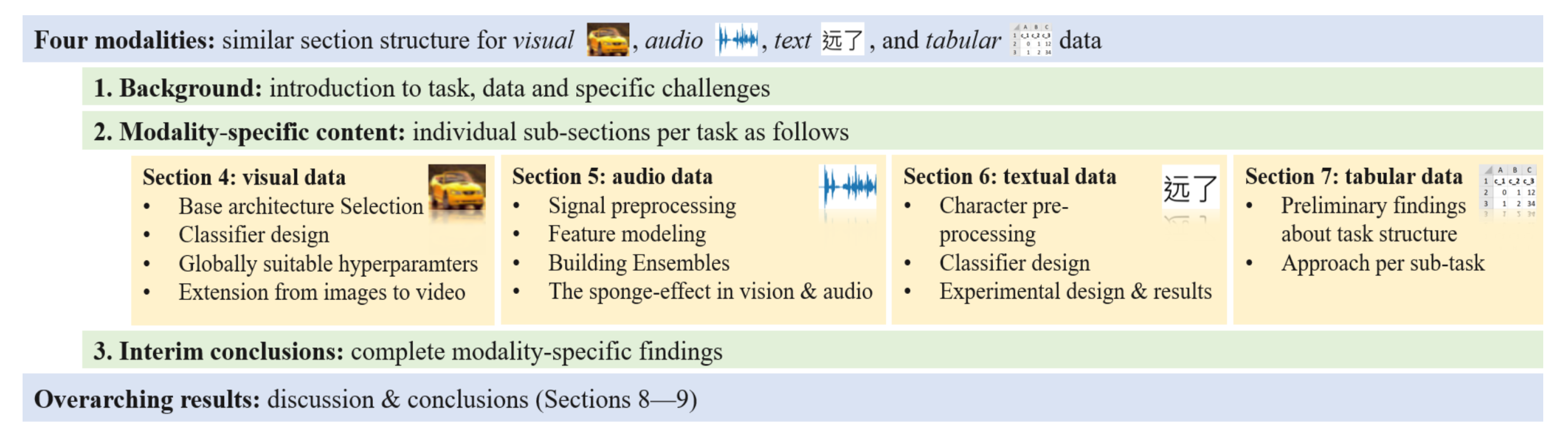
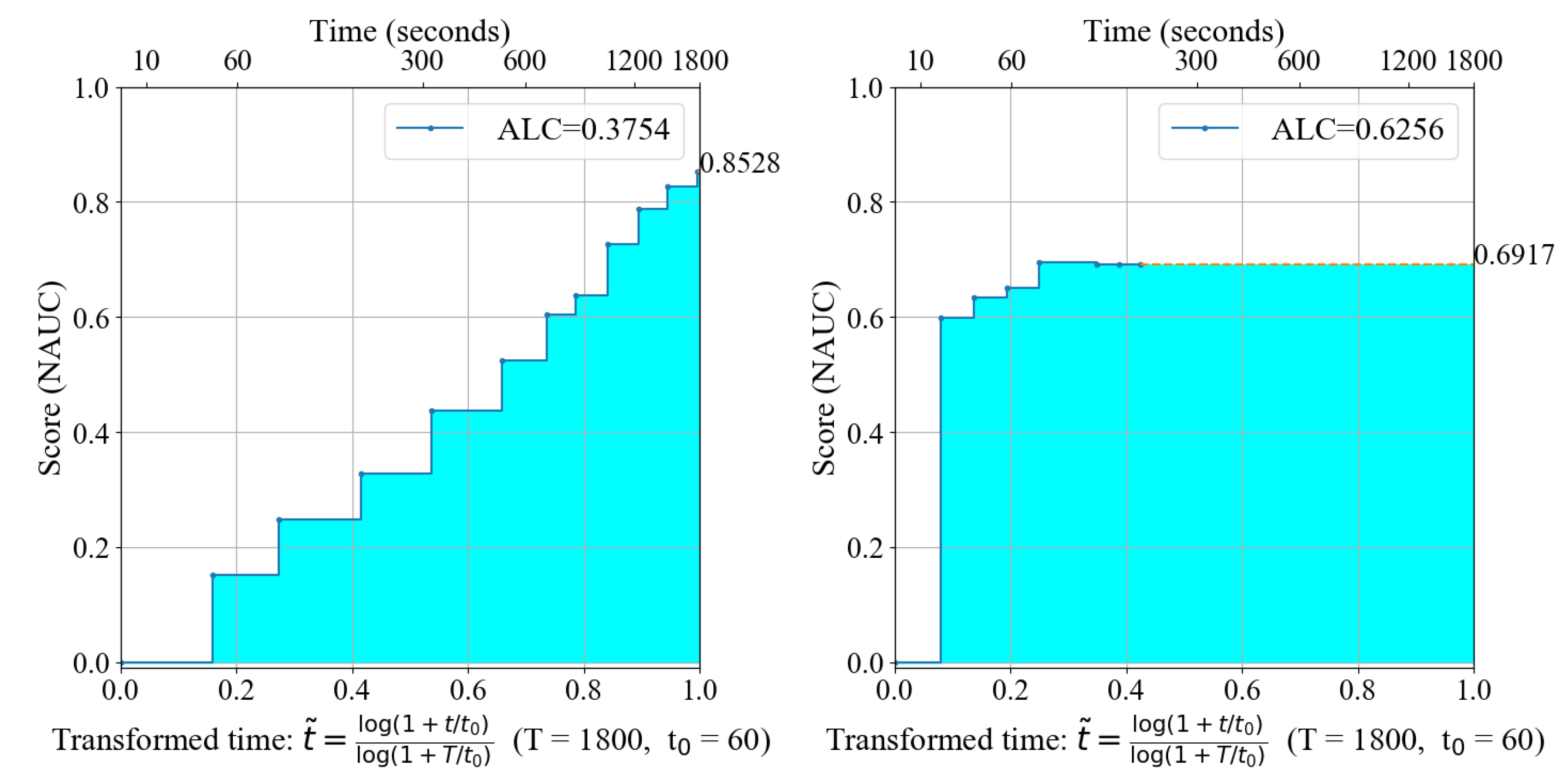
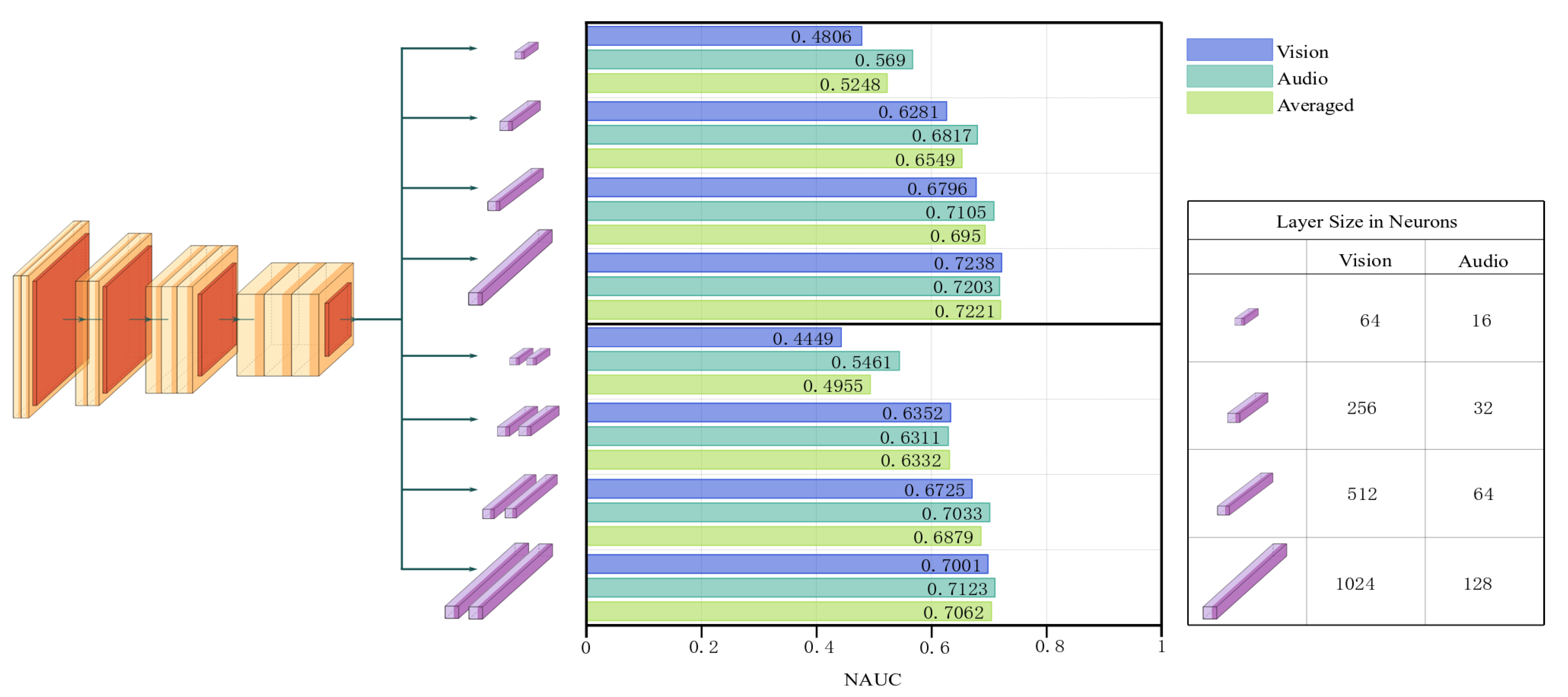
Table 1.
Vision: Summary of vision datasets.
| Dataset | Content | Modality | Size | No. Training Samples | No. Classes |
|---|---|---|---|---|---|
| Chucky | Everyday Objects | Images | 48,061 | 100 | |
| Decal | Satellite Images | Images | Varying | 634 | 11 |
| Hammer | Medical Images | Images | 8050 | 7 | |
| Pedro | Pedestrian Images | Images | Varying | 80,095 | 26 |
| Katze | Common Actions | Videos | 1528 | 6 | |
| Kraut | Common Actions | Videos | 1528 | 4 | |
| Kreatur | Common Actions | Videos | 1528 | 6 |
Table 2.
Vision: Numerical evaluation of different network architectures on the image and video training datasets.
Table 2.
Vision: Numerical evaluation of different network architectures on the image and video training datasets.
| Datatype | Image | Video | ||||||
|---|---|---|---|---|---|---|---|---|
| Dataset | Chucky | Decal | Hammer | Pedro | Katze | Kraut | Kreatur | |
| MobileNetV2 | Return Time (s) | |||||||
| ALC | ||||||||
| NAUC | ||||||||
| Overfit? | Yes | Minor | No | No | No | No | No | |
| EfficientNet-mini | Return Time (s) | |||||||
| ALC | ||||||||
| NAUC | ||||||||
| Overfit? | Yes | Minor | No | No | No | No | No | |
| EfficientNet B0 | Return Time (s) | |||||||
| ALC | ||||||||
| NAUC | ||||||||
| Overfit? | Yes | Yes | No | No | No | No | No | |
Table 3.
Vision: Comparison of different pooling methods for image and video classification, using the MobileNetv2 architecture.
Table 3.
Vision: Comparison of different pooling methods for image and video classification, using the MobileNetv2 architecture.
| Datatype | Image | Video | ||||||||||||
|---|---|---|---|---|---|---|---|---|---|---|---|---|---|---|
| Dataset | Chucky | Decal | Hammer | Pedro | Katze | Kraut | Kreatur | |||||||
| Measure | ALC | NAUC | ALC | NAUC | ALC | NAUC | ALC | NAUC | ALC | NAUC | ALC | NAUC | ALC | NAUC |
| Flatten | ||||||||||||||
| Spat. pooling | ||||||||||||||
| Tmp. pooling | − | − | − | − | − | − | − | − | ||||||
| Spat. & tmp. | − | − | − | − | − | − | − | − | ||||||
Table 4.
Vision: ALC performance of the evaluated video classification models for the various video datasets.
Table 4.
Vision: ALC performance of the evaluated video classification models for the various video datasets.
| Model | 2+1D | 2+1D Small | Late 3D |
|---|---|---|---|
| Kreatur | |||
| Katze | |||
| Kraut | − |
Table 5.
Audio: Summary of audio datasets.
| Avg. | Max. | Min. | |||
|---|---|---|---|---|---|
| Dataset | Classes | Length (s) | Length (s) | Length (s) | Samples |
| Speaker | 100 | 3000 | |||
| Emotion | 7 | 428 | |||
| Accent | 3 | 976 | |||
| Genre | 20 | 939 | |||
| Language | 10 | 199 |
Table 6.
Audio: List of parameters used to compute Mel-spectrograms and MFCCs.
| LibROSA | Speaker | Empirically | |
|---|---|---|---|
| Parameter | Default [77] | Clust. [78] | Optimal |
| Audio segment length (s) | or 3 | 3 | |
| Down sampling rate | 1 | 2 | 1 |
| Proc. sampling rate (kHz) | 16 | 8 | 16 |
| Frame length | 2048 | 256 | 2048 |
| Hop length | 512 | 128 | 512 |
| FFT length (samples) | 2048 | 512 | 2048 |
| Number of Mel bins | 40 or 128 | 128 | 128 |
| Number of Mel features | 40 | 24 | 24 |
| Lower/upper edge freq. (Hz) |
Table 7.
Audio: Performance of various architectures on the training datasets.
| Speaker | Emotion | Accent | Music | Language | ||
|---|---|---|---|---|---|---|
| Model | Metric | Identification | Recognition | Detection | Genre | Classification |
| MFCCs + GRUs | ALC | |||||
| NBAC | ||||||
| CNNs + Global pooling | ALC | |||||
| NBAC | ||||||
| VGGish [74] | ALC | |||||
| NBAC |
Table 8.
Audio: Performance of a sequential and a parallel ensemble on the training datasets.
| Speaker | Emotion | Accent | Music | Language | ||
|---|---|---|---|---|---|---|
| Ensemble Type | Metric | Identification | Recognition | Detection | Genre | Classification |
| Sequential | ALC | |||||
| NAUC | ||||||
| Parallel | ALC | |||||
| NAUC |
Table 9.
Text: Characteristics of the used textual datasets; ACI refers to the average number of characters per instance.
Table 9.
Text: Characteristics of the used textual datasets; ACI refers to the average number of characters per instance.
| Name | Language | Domain | # Train | # Test | ACI | # Classes |
|---|---|---|---|---|---|---|
| DEMO | ZH | Hotel Reviews | 6k | 4k | 2 | |
| O1 | EN | Movie Reviews | 7k | 2k | 2 | |
| O2 | EN | News Groups | 11k | 7k | 20 | |
| O3 | EN | Enron Mails | 60k | 50k | 2 | |
| O4 | ZH | Short News | 55k | 10k | 10 | |
| O5 | ZH | Product Teasers | 156k | 72k | 18 |
Table 10.
Text: ALC and NAUC performance of evaluated text classification models. Best performances are marked in bold.
Table 10.
Text: ALC and NAUC performance of evaluated text classification models. Best performances are marked in bold.
| Dataset | DEMO-ZH | O1-EN | O2-EN | O3-EN | O4-ZH | O5-ZH | ||||||
|---|---|---|---|---|---|---|---|---|---|---|---|---|
| Metric | ALC | NAUC | ALC | NAUC | ALC | NAUC | ALC | NAUC | ALC | NAUC | ALC | NAUC |
| CNN | ||||||||||||
| SVM 1-GRAM | ||||||||||||
| SVM 1-GRAM Logits | ||||||||||||
| SVM N-GRAM | NA | NA | ||||||||||
| BERT | NA | NA | ||||||||||
| SVM N-GRAM Iterative | ||||||||||||
| SVM fasttext | ||||||||||||
| DeepBlueAI | ||||||||||||
| Upwindflys | ||||||||||||
| TXTA | ||||||||||||
Table 11.
Text: Average rank over ALC, for all datasets and per language; Corr-char: correlation between rank and average number of characters per sample.
Table 11.
Text: Average rank over ALC, for all datasets and per language; Corr-char: correlation between rank and average number of characters per sample.
| Language | ALL | EN | ZH | Corr-Char |
|---|---|---|---|---|
| CNN | ||||
| SVM 1-GRAM | ||||
| SVM 1-GRAM Logits | ||||
| SVM N-GRAM | ||||
| BERT | ||||
| SVM N-GRAM Iterative | ||||
| SVM fasttext | ||||
| DeepBlueAI | ||||
| Upwindflys | ||||
| TXTA |
Table 12.
Tabular: Brief overview of ingredients used by leading submissions in the AutoWSL competition.
Table 12.
Tabular: Brief overview of ingredients used by leading submissions in the AutoWSL competition.
| Team (Rank) | PU and Semi-Supervised Learning Tasks | Learning on Noisy Data | |||||
|---|---|---|---|---|---|---|---|
| LightGBM | Using a Meta-Classifier to Generate Labels for Unlabeled Data | Learning Importance of Each Feature Using a Metamodel | LightGBM | Data Cleaning for Learning on Noisy Labels | Using an Ensemble of Extremely Weak Classifiers | Down-Weighing and Removal of Potentially Noisy Data | |
| DeepWisdom (1) | ✔ | ✔ | ✔ | ||||
| Meta_Learners (2) | ✔ | ✔ | ✔ | ||||
| lhg1992 (3) | ✔ | ✔ | ✔ | ✔ | |||
| Ours (6) | ✔ | ✔ | ✔ | ✔ | |||
Table 13.
Discussion: Overview of the identified patterns in the evaluations throughout this paper.
| Modality | Finding | Section(s) |
|---|---|---|
| Images | MobileNetV2 is preferred over EfficientNet in a resource constrained environment for simple datasets | Section 4.2 |
| Images, Video | Spatial pooling is preferred over flattening or temporal pooling | Section 4.3 |
| Images, Audio | Increasing the size of the fully connected classifier increases the sample efficiency of the model | Section 4.3 and Section 5.6 |
| Audio | Audio preprocessing hyperparameters are non-universal | Section 5.2 |
| Audio | Architecture search is preferred in model design for small datasets | Section 5.3 |
| Audio | Small sized datasets allow using model ensembles even under resource constraints | Section 5.4 |
| Text | The hashing trick allows for fast computation of TF-IDF | Section 6.2 |
| Text | In NLP neither SVM nor deep-learning or hybrid systems are clearly superior | Section 6.4 |
| Text | The use of multiple n-gram ranges consistently improves final performance | Section 6.4 |
| Text | The use of multiple CNN blocks in parallel clearly improves anytime performance | Section 6.4 |
| Text | SVMs work better on long texts while deep learning is superior on short text samples | Section 6.5 |
| Tabular | Decision tree-based methods in a weakly supervised setting are extremely dependent on good hyperparameters | Section 7.2 |
| Tabular | Sample selection for pseudo-labeling has to be carefully tuned not to be too slow (no progress) or too fast (degrading performance) | Section 7.2 |
| Tabular | A combination of boosting and very weak LightGBM classifiers works best for noisy labels | Section 7.2 |
| Tabular | Shallow machine learning is still very relevant especially in data- and computing-constrained scenarios | Section 7.4 |
Publisher’s Note: MDPI stays neutral with regard to jurisdictional claims in published maps and institutional affiliations. |
© 2020 by the authors. Licensee MDPI, Basel, Switzerland. This article is an open access article distributed under the terms and conditions of the Creative Commons Attribution (CC BY) license (http://creativecommons.org/licenses/by/4.0/).
Share and Cite
MDPI and ACS Style
Tuggener, L.; Amirian, M.; Benites, F.; von Däniken, P.; Gupta, P.; Schilling, F.-P.; Stadelmann, T. Design Patterns for Resource-Constrained Automated Deep-Learning Methods. AI 2020, 1, 510-538. https://doi.org/10.3390/ai1040031
AMA Style
Tuggener L, Amirian M, Benites F, von Däniken P, Gupta P, Schilling F-P, Stadelmann T. Design Patterns for Resource-Constrained Automated Deep-Learning Methods. AI. 2020; 1(4):510-538. https://doi.org/10.3390/ai1040031
Chicago/Turabian StyleTuggener, Lukas, Mohammadreza Amirian, Fernando Benites, Pius von Däniken, Prakhar Gupta, Frank-Peter Schilling, and Thilo Stadelmann. 2020. "Design Patterns for Resource-Constrained Automated Deep-Learning Methods" AI 1, no. 4: 510-538. https://doi.org/10.3390/ai1040031