Deep Learning for Lung Cancer Nodules Detection and Classification in CT Scans


1
Perception, Robotics, and Intelligent Machines (PRIME), Department of Computer Science, Université de Moncton, Moncton, NB E1A3E9, Canada
2
Department of Electronic Engineering, Universidad Técnica Federico Santa Maria, Valparaiso, Chile
*
Author to whom correspondence should be addressed.
†
These authors contributed equally to this work.
AI 2020, 1(1), 28-67; https://doi.org/10.3390/ai1010003
Submission received: 10 December 2019
/
Revised: 31 December 2019
/
Accepted: 3 January 2020
/
Published: 8 January 2020
(This article belongs to the Section Medical & Healthcare AI)
Abstract
:Detecting malignant lung nodules from computed tomography (CT) scans is a hard and time-consuming task for radiologists. To alleviate this burden, computer-aided diagnosis (CAD) systems have been proposed. In recent years, deep learning approaches have shown impressive results outperforming classical methods in various fields. Nowadays, researchers are trying different deep learning techniques to increase the performance of CAD systems in lung cancer screening with computed tomography. In this work, we review recent state-of-the-art deep learning algorithms and architectures proposed as CAD systems for lung cancer detection. They are divided into two categories—(1) Nodule detection systems, which from the original CT scan detect candidate nodules; and (2) False positive reduction systems, which from a set of given candidate nodules classify them into benign or malignant tumors. The main characteristics of the different techniques are presented, and their performance is analyzed. The CT lung datasets available for research are also introduced. Comparison between the different techniques is presented and discussed.

1. Introduction
Lung cancer is considered as the deadliest cancer worldwide. For this reason, many countries are developing strategies for the early diagnosis of lung cancer. The NLST trial [1], showed that three annual screening rounds of high-risk subjects using low-dose Computed Tomography (CT) reduce the death rates considerably [2]. These measures mean that an overwhelming quantity of CT scan images will have to be inspected by a radiologist. Since nodules are very difficult to detect, even for experienced doctors, the burden on radiologists increases heavily with the number of CT scans to analyze.
With the expected increase in the number of preventive/early-detection measures, scientists are working in computerized solutions that help alleviate the work of doctors, improve diagnostics’ precision by reducing the subjectivity factor, speedup the analysis and reduce medical costs.
In order to detect malignant nodules, specific features need to be recognized and measured. Based on the detected features and their combination, cancer probability can be assessed. However, this task is very difficult, even for an experienced medical doctor, since nodule presence and positive cancer diagnosis are not easily related. Common computer aided diagnosis (CAD) approaches use previously studied features which are somehow related to cancer suspiciousness, such as volume, shape, subtlety, solidity, spiculation, sphericity, among others. They use these features and Machine Learning (ML) techniques such as Support Vector Machine (SVM) to classify the nodule as benign or malignant. Even though many works use similar machine learning frameworks [3,4,5,6,7,8], the problem with these methods is that, in order for the system to work at its best performance, many parameters need to be hand-crafted, thus making it difficult to reproduce state-of-the-art results. Additionally, this makes these approaches vulnerable to the variability between different CT scans and different screening parameters.
The advantage of using deep learning in CAD systems is that it can perform and end-to-end detection by learning the most salient features during training. This allows the network to be robust to variations as it captures nodules’ features in various CT scans with varying parameters. By having a training set which is rich in variability, the system can inherently learn invariant features from malignant nodules and enables better performances. Since no features are engineered, the network is able to learn, on its own, the relation between features and cancer using the provided ground-truth. Once the network is trained, it is expected to be able to generalize its learning and detect malignant nodules (or patient-level cancer) on new cases which have never been seen before by the system.
In this work, we present a review of recent deep learning techniques for lung cancer detection. Most of the proposed works are based on deep Convolutional Neural Networks (CNN). CNN are a class of neural networks designed to learn, during training, convolution parameters from a set of available data. In general, they are comprised of different layers such as convolutional layers, deconvolutional layers, pooling layers and so forth. Different architectures were proposed in recent years to improve the performance and overcome some limitations of the standard CNN. Among them Residual Networks (ResNets) [9], Inception [10,11], Xception [12] or Dense Networks [13,14]. CNN have shown interesting performances in the tasks of classification, segmentation, object detection and so forth. Mainly applied to image data, they have been successfully used with other type of data such as text in NLP applications [15]. More details about deep learning and CNN are given in Reference [16]. In the following, we will present the main datasets used in lung cancer research (Section 2) and introduce the common metrics used to assess the deep learning models (Section 3). The techniques are divided into two categories—Nodule detection frameworks (Section 4) and false positive reduction models (Section 5). Comparative analysis of the different algorithms is presented and discussed (Section 6).
2. Datasets
Datasets are an important part of any machine learning or deep learning approach. The quality of the available data help develop, train and improve the algorithms. In medical imaging applications, the available data must be validated and labeled by experts in order to be useful in any development. This section present the datasets used in recent works related to deep learning for lung cancer detection.
2.1. The Lung Image Database Consortium (LIDC-IDRI)
The LIDC-IDRI dataset [17] consists of 1018 cases gathered from a collaboration of seven academic centers and eight medical imaging companies. Each case includes an XML file containing annotations of the CT scan. These annotations are performed by four experienced thoracic radiologists, in a 2-stage process. In the first stage, each radiologist independently categorizes findings into three categories (nodule ≥ 3 mm, nodule ≤ 3 mm and non-nodule ≥ 3 mm). Then, in the second stage, each radiologist reviews its classification and the classifications done by the other radiologists anonymously. So every nodule annotation is reviewed by all four radiologists independently.
The dataset consists of 1018 CT scans from 1010 patients, with a total of 244,527 images. With this dataset, the diagnosis can be made at two levels. Diagnosis at the patient level (diagnosis associated with the patient) and diagnosis at the nodule level.
The CT scan DICOM images have a resolution of 512 × 512 × width, where the width varies from 65 to 764 slices. The average number of slices width is 240 for this dataset.
The nodules are categorized into 4 levels. (1) Unknown (no data available), (2) Benign or non-malignant disease, (3) A malignancy that is primary lung cancer, (4) A metastatic lesion that is associated with an extra-thoracic primary malignancy. Furthermore, for each lesion, there is also information available about how the diagnosis was established. Including options as (1) Unknown (not clear how the diagnosis was established), (2) review of radiological images to show 2 years of stable nodule, (3) biopsy, (4) surgical resection and (5) progression or response [18].
2.2. LUNA16
The LUNA16 dataset [19] is a subset of LIDC-IDRI dataset, in which the heterogeneous scans are filtered by different criteria. Since pulmonary nodules can be very small, a thin slice should be chosen. Therefore scans with a slice thickness greater than 2.5 mm were discarded. Furthermore, scans with inconsistent slice spacing or missing slices were also excluded. This led to 888 CT scans, with a total of 36,378 annotations by radiologists. In this dataset, only the annotations categorized as nodules ≥ 3 mm are considered relevant, as the other annotations (nodules ≤ 3 mm and non-nodules) are not considered relevant for lung cancer screening protocols [2]. Nodules found by different readers that were closer than the sum of their radii were merged. In this case, positions and diameters of these merged annotations were averaged. This results in a set of 2290, 1602, 1186 and 777 nodules annotated by at least 1, 2, 3 or 4 radiologist, respectively.
In Figure 1, different slices from a LUNA16 CT scan with malignant nodules are shown as an example of a Lung CT scan. For the other datasets, the same kind of image is obtained.
Figure 2 shows how similar are the benign and the malignant lesions. Thus, revealing the hard task of classifying them.
2.3. SPIE-AAPM-NCI LungX
This dataset [20] was built for a challenge sponsored by SPIE, AAPM, NCI and investigators from the University of Chicago, University of Michigan and Oak Ridge National Laboratory. The objective of this challenge was the computerized classification of lung nodules as benign or malignant in CT scans. The DICOM images were divided into a calibration and testing phase. The calibration set consisted of 10 thoracic CT scans, five containing a single confirmed benign nodule and five with a single confirmed malignant nodule. The annotations contained the location of the nodule and the diagnosis as benign or malignant. The test set contained 60 thoracic CT scans with a total of 73 nodules (13 scans contained two nodules each). Annotations were provided in which the location of the nodule is indicated.
2.4. National Lung Screening Trial (NLST)
The National Lung Screening Trial (NLST) [1] was a randomized controlled clinical trial of screening tests for lung cancer. Approximately 54,000 participants were enrolled between August 2002 and April 2004. Participants were randomly assigned to two study arms in equal proportions. One arm received low-dose helical computed tomography (CT), while the other received single-view chest radiography. Participants were offered three exams (T0, T1 and T2) at one-year intervals, with the first (T0) performed soon after entry. The goal of the study was to assess whether low-dose CT screening reduces lung cancer mortality among high-risk individuals compared to chest radiography. Data were collected on cancer diagnoses and deaths that occurred through 31 December 2009. NLST was a collaborative effort of the National Cancer Institute’s Division of Cancer Prevention (DCP) and Division of Cancer Treatment and Diagnosis (DCTD). A positive screening result (suspicious for lung cancer) was assigned if any non-calcified nodules or masses ≥ 4 mm in diameter were noted or if any other abnormalities were judged suspicious for lung cancer by the radiologist. Three types of negative screening results were possible: clinically significant abnormalities not suspicious for lung cancer, minor abnormalities not suspicious for lung cancer and no significant abnormalities.
2.5. Automatic Nodule Detection (ANODE09)
This dataset [21] was provided by the Nelson study, which is the largest CT lung cancer screening trial in Europe. Each scan contains annotations of the findings, including spatial location and the type of finding—label 1 for the true nodule and label 2 for irrelevant finding (which is not cancer-related). The dataset contains 55 CT scans. Annotations are available for 5 examples. For the remaining scans, annotations are not publicly available since they are used for testing the performance of CAD systems. Findings were divided into four groups in Nelson’s study [22]. Class 1 contained nodules with fat, benign calcifications or other benign characteristics. The other groups contained nodules without benign characteristics. Class 2 nodules had a volume below 50 mm. Class 3 contained solid, part-solid or non-solid nodules with a volume between 50 and 500 mm. Larger nodules fell into class 4 and participants with such a nodule were referred to a pulmonologist for diagnosis.
2.6. The Danish Lung Cancer Screening Trial (DLCST)
The Danish Lung Cancer Screening Trial [23] assessed participants with high lung cancer risk. Two experienced chest radiologists evaluated the images, where size was manually measured. A nodule diameter of 3 mm was considered the lower limit of a positive finding in the initial evaluation. A chest radiologist, unaware of lung cancer diagnoses, recorded spiculation and malignancy observations and categorized the nodules according to type—perifissural, solid, part-solid or non-solid (pure ground glass). This yielded to 823 patients with 1385 diagnosed nodules of which 233 nodules were classified as benign calcification and excluded, leaving a total of 718 persons and 1152 nodules [24].
2.7. Data Science Bowl 2017 (DSB)
The Data Science Bowl 2017 (DSB), a challenge organized by Kaggle [25], released a database of CT scans on two stages, DSB1 and DSB2. This dataset provides annotations at a patient level, indicating whether the patient was diagnosed with cancer within one year after the scan was taken. It contains over a thousand low-dose CT scan images in a DICOM format from high-risk patients. This database is not publicly available at the moment due to usage restrictions. DSB scan resolutions and scan parameters vary in source and quality. The source of the CT scans was not released. This might generate problems when using this dataset, for both training or testing. Because, if the model is assessed on other datasets, it is not possible to know if samples from those data are already included in the DSB dataset.
Table 1 summarizes the datasets used for developing deep learning lung cancer detection algorithms.t
3. Performance Metrics
To analyze the performance of the developed deep learning algorithms for detecting and classifying lung nodules, different metrics are used. In the reviewed papers, the authors use statistical measures [26] such as sensitivity (SE), specificity (SP), accuracy (ACC), precision (PPV), F1-score, Receiver Operating Characteristic (ROC) curve, Free Response Operating Characteristic (FROC) and area under the ROC curve (AUC). Another measure was introduced in the ANODE09 challenge and was later used in the LUNA16 Challenge to assess the performance of the different models, this measure is the Competition Performance Metric (CPM) [21]. The different metrics used in assessing the performance of lung cancer algorithms are given in Table 2.
4. Deep Nodule Detection Frameworks
Due to the complexity of detecting pulmonary nodules and the importance of trying to detect all of them, the typical framework is divided into two main tasks. The first one focuses on detecting nodule candidates. This tries to detect from the CT scan volume all the true nodules, which usually includes a high number of false positives. Then, the second task specializes in classifying the previously generated candidates into benign nodules or malignant nodules. The second step basically aims to reduce the large number of false positives generated on the previous step. Some works do not use this strategy and from the CT scans they detect and classify nodules directly.
In this section, we present works which propose a whole pipeline from the CT scans to the final classification of the detected nodules. As aforementioned, some of them divide the task into candidate generation and false positive reduction, while other do not. Different works may differ in architecture, pre-processing of the images, training strategy, among others. A relevant difference between approaches is if they are using a two-dimensional or three-dimensional approach. 3D architectures demand the use of three-dimensional convolutions, which increases considerably the number of parameters, the computational cost and the training time. For this reason, some approaches use 2D convolutions, which have fewer parameters and allow to train deeper and more complex architectures with less powerful hardware. 2D and 3D approaches are presented in the following.
4.1. 2D Deep Learning Approaches
Here we present works that are based on a 2D approach. This means that two-dimensional kernels are convoluted with two-dimensional images or that the input of the deep neural network is two-dimensional. This does not necessarily means that these architectures miss out all 3D information. Some approaches make use of adjacent slices or different axial cuts in order to retain some volumetric information.
Van Ginneken et al. [27] propose the use of transfer learning from OverFeat [28], a previously trained network for object detection in natural images. First, from the CT scan they extract 2D sagittal, coronal and axial patches for each nodule candidate. Then, they extract 4096 features from the penultimate layer of the network and classify them with linear SVM. Each patch is 50 × 50 mm and rescaled to 8-bit grayscale 221 × 221 pixels using Hounsfield unit rescaling and linear interpolation. They use 865 scans from the LIDC dataset, considering nodules ≥ 3 mm labeled by 3 or 4 radiologists as positive samples. Scan with a section thickness of more than 2.5 mm is excluded as well as scans with inconsistent or invalid DICOM. This results in 865 CT scans with 1147 pulmonary nodules and 3271 excluded doubtful lesions. As the starting point of this framework, nodule candidate’s locations are extracted from an existing CAD system approved by the U.S. Food and Drug Administration (FDA) [29] and commercially available (MeVis Medical Solutions AG, Bremen, Germany). The CAD system produces a list of candidates, each with a score indicating the likelihood that the location is a nodule. The OverFeat network uses a 221 × 221 RGB image patch as input. It consists of Convolutional Layers (CL) containing 96 to 1024 kernels of sizes 3 × 3 to 7 × 7. It uses half-wave rectification and max-pooling kernels of sizes 3 × 3 and 5 × 5. The resulting 4096 features from the first Fully Connected (FC) layer are used as input to the linear Support Vector Machine (SVM) classifier with C optimized cross-validation [30]. The authors constructed three separate systems, one for each orthogonal patch, designated x, y and z. To fuse these results, the best performing model was a late fusion approach using the CAD information. This was done by using the output of the three systems x, y, z plus the score reported by the CAD system. Then, they use a second stage classifier (linear SVM) to estimate the probability that the candidate is a nodule. The CAD system by itself generated 37,262 candidate locations. Among those candidates 78% were true nodules (i.e, the maximum sensitivity the study could achieve). The complete model achieves a CPM of 0.71.
Kumar et al. [31] propose a CAD system that uses deep features extracted from an autoencoder to classify lung nodules. They use CT scans from patients with diagnostic data from the LIDC dataset. There are 157 patients with diagnostic information obtained from biopsy, surgical resection, progression or reviewing the radiological images to show 2 years of nodule state at two levels (the patient level and the nodule level). They decided to use diagnostic data since it is the only way to judge the certainty of malignancy. First, nodules are extracted from the 2D CT images using the annotations provided in the dataset. Then they are individually fed into a five-layered de-noising autoencoder trained by L-BFGS [32]. Learned features are then extracted from the 4th layer. The features from the 4th layer were used to create a feature vector of 200 dimensions for each instance (instance meaning one slice containing nodules). Then this vector is fed into a binary decision tree to obtain the classification for nodules. For each nodule ≥ 3 mm in diameter, the annotations provided by the radiologist are used to extract features from the autoencoder. They created an adaptive rectangle window based on the nodule size. Then each rectangular area is resized to a fixed dimension, to create a fixed length input for the autoencoder. Nodules with rating 0, 2, 3 are treated as malignant. They achieved an overall accuracy of 75.01% with a sensitivity of 0.8325 at a 0.39 FP/scan.
In Reference [33], the authors use two models based on Deep Belief Networks (DBN) and Convolutional Neural Networks (CNN), respectively. The authors used the LIDC dataset where the training samples were resized to 32 × 32 ROIs. For the DBN they used the strategy proposed by Hinton et al. [34], which consists of a greedy layer-wise unsupervised learning algorithm for DBN. Figure 3 shows the learning framework, where RBM (Restricted Boltzmann Machine) is trained with stochastic gradient descent. For the CNN, the dimensionality of the Convolutional layers is set as 2 to capture local spatial patterns. A sigmoid is used as an activation function and max-pooling to reduce the dimensionality. They use 4 feature maps for the first layer followed by 6 features maps, finally a FC layer is used to classify the nodule. The DBN is first trained in an unsupervised fashion to get a preliminary model. Then it is fine-tuned in a supervised process for the classification task. The DBN trains one layer at a time, from the bottom-up. The training is based on the stochastic gradient descent method and the contractive divergence algorithm to approximate the maximum log-likelihood. The DBN achieves a sensitivity of 0.734 and a specificity of 0.822. While the CNN achieves a sensitivity of 0.733 and a specificity of 0.787.
Another work using DBNs and CNNs is proposed by Sun et al. [35]. In this work, the authors implement three different deep learning approaches. Using cropped 52 × 52 pixels patches from the LIDC database, they trained and tested CNN, DBNs and Stacked Denoising Autoencoder (SDAE) [36]. The proposed CNN consists of 3 CL, each one with max-pooling. 5 × 5 kernels were used to generate 12, 8 and 6 features maps, respectively. The second network is a DBN. It was obtained by training and stacking four layers of RBM in a greedy fashion. Each layer contained 100 RBM. The trained stack was used to initialize a feed-forward neural network for classification. The hyperbolic tangent () was used as an activation function. The last model was a three-layer SDAE, where each autoencoder was stacked on top of each other. Each autoencoder has 2000, 1000 and 400 hidden neurons, with corruption level of 0.5. From the 5 levels of malignancy available in the LIDC dataset (annotated by experts), they considered benign the ones with levels 1 and 2, while the 4 and 5 were considered malignant cases. The level 3 nodules were eliminated. For each nodule, they averaged the ratings from the four radiologists. For every nodule, its area was segmented based on the union of the four radiologists’ truth files. If the segmented area fits into 52 × 52 pixels, this ROI was placed at the center of the box. The ones that exceeded this size were downsampled to the reference size of 52 × 52 pixels. Then each ROI was rotated to four different directions and each rotated ROI was converted into four single vectors. The pixel values were converted to 8 bits. With this preprocessing, from the 1018 cases 174,412 vectors were generated. Each vector with 2704 elements. After discarding the level 3 nodules, 114,728 vectors remained, consisting of 54,880 benign cases and 59,848 malignant cases. The performance of the proposed algorithms were assessed on accuracy where CNN, DBNs and SDAE achieved 0.7976, 0.8119 and 0.7929, respectively.
The framework in Reference [37] uses an architecture based on the popular deep object detector called YOLO (You Only Look Once) [38]. YOLO is used to detect nodules in CT scans. A regression problem is optimized with a single CNN simultaneously predicting multiple bounding boxes and class probabilities for those boxes. The input is divided into a regular grid, with spacing slightly smaller than the smallest object expected for detection (smallest nodule). Each grid square has a label associated with it (the class of the object it contains) and the pixel coordinates of the bounding box. The grid square in which the center of an object falls is responsible for detecting that object. When multiple objects are present in the same grid square, the network selects the object which covers the maximum number of pixels within the grid. Features obtained from the entire image are used to predict each bounding box, allowing the network to learn the objects in the full image. The network architecture and workflow for the training and validation processes used in DetectNet are shown in Figure 4a,b. Both object classification and regression are performed at the same time to estimate object bounding boxes, which give a higher inference performance than an ordinary classifier applied in a sliding window manner. The fully convolutional layer of DetectNet has the same structure as GoogLeNet [39] which has 22 layers. The inception module of GoogLeNet concatenates filters of different sizes and dimensions into a single new filter. GoogLeNet has two convolution layers, two pooling layers and nine Inception layers. Each inception layer consists of six convolution layers and one pooling layer. Data input layers, final pooling layer and the output layers of GoogLeNet are eliminated from DetectNet. The architecture is shown in Figure 4c. There are no FC layers, this allows the network to accept input images with varying sizes and the CNN can be applied in a sliding window fashion with appropriate strides. The CNN has a receptive field of 555 × 555 pixels and a stride of 16 pixels. The system is evaluated on the LIDC dataset. It takes advantage of depth information by including CT slices as RGB channels. Also, it makes use of transfer learning by using the weights of a pre-trained object detection network. Online augmentation is performed in the training set extracted from LIDC-IDRI database, consisting of pixel shifts and flips. Level 2 of agreement is used for nodules and only the ones with a diameter between 3 mm and 30 mm are used. 3300 images containing nodules met these requirements. Non-linear contrast enhancement was performed as preprocessing. CT scans were resized to 1024 × 1024 using bicubic interpolation. DetectNet uses a linear combination of two separate loss functions to produce its final loss, coverage loss and L1 loss of the predicted and true bounding boxes. The system achieves 0.89 sensitivity at 6 false positives per image on the LIDC database and a precision of 0.93.
Trajanovski et al. [40] present a two-stage framework, in which the first part employs a nodule detector based on SVM. The second stage uses both contextual information about the nodule and nodule features as input to a CNN, inspired by a ResNet architecture, to estimate the malignancy risk of the whole CT scan. This approach uses a multi-instance weakly-labeled method to train the model, which only requires cancer diagnosis confirmed at the patient level. It is trained on heterogeneous data sources (NLST, LHMC and DSB). The first stage uses a nodule detector to localize nodules in CT scans. Then the 10 largest nodules are used as input for the second stage, which consists of a deep and wide neural network, to evaluate the risk of cancer. For the nodule detection algorithm, an SVM-based nodule detector is used with multi-thresholding to get a robust detection that tries to contain all true nodules while reducing the number of irrelevant findings. To reduce the number of found candidates a cascaded SVM strategy is used. First, the lung is segmented to limit the search on the volume of interest. Then iso-contours are used to find bright circular or semi-circular objects and a binary image with a corresponding distance map is computed. Two-dimensional seed points are created at all ridge points in the distance map. Finally, based on multiple 3D iso-surfaces around each seed, only the 3D-sphere-like objects are kept. To reduce the high number of false positives, detected in the previous step, a hierarchical SVM strategy is used with 35 image features containing geometric features, grayscale features, location features, as well as image properties. From these features, a first SVM is trained. Then, from the remaining candidates, a second SVM is trained. This approach yielded to a sensitivity of 0.859 at 2.5 FPs/scan evaluated on the LIDC-IDRI dataset. The Deep Neural Network for cancer risk assessment uses the information obtained by the nodule detection step, which provides candidates with indications about the location, nodule size, nodule sphericity and confidence of suggestion. These are referred to as metadata. Then, patches of size 32 × 32 × 32 mm are extracted around the nodule. Isotropic resampling was used to make every voxel correspond to 1 mm. During training, a random crop of 28 × 28 × 28 mm is extracted from the patch on every batch iteration to avoid overfitting. Finally, from the 3D patches, 3 different orthogonal 2D projections are extracted as channels, resulting on a 3 × 28 × 28 mm input for the network. To further improve the performance, the metadata is added at the penultimate layer of the architecture. The deep network is a ResNet-like deep and wide model. It uses sigmoid activation function. At the end of the network a global max-pooling is performed, over the maximum of ten branches representing the different nodules, to estimates the final cancer risk probability. The model was trained on a subset of the NLST data (3410 volumes, with 680 diagnosed cancer cases). It was verified on NLST and other datasets. AUC scores for the model, evaluated against confirmed cancer diagnosis, range from 0.82 to 0.88. The AUC on LHMC, UCM, NLST validation set, DSB 1 and DSB 2, are 0.87, 0.83, 0.88, 0.82 and 0.84, respectively.
The work in Reference [41] fuses texture, shape and deep model-learned information (Fuse-TSD) for automated classification of lung nodules. The algorithm uses three types of features extracted using gray level co-occurrence matrix (GLCM) texture descriptors and Fourier shape descriptors to characterize the heterogeneity of nodules and a DCNN to learn features of nodules on a slice-by-slice basis. An ensemble classifier based on back-propagation neural network (BPNN) and AdaBoost is constructed. The decisions made by the different classifiers are fused by a weighted sum of likelihood, where the weights are proportional to the accuracy recorded on the validation set. A 64 × 64 square region centered on the nodule is cropped (the largest nodule is 64 mm). The area of the nodule is defined as the intersection of the marked areas by the four radiologists. The non-nodule voxels are set to zero. For DCNN-based feature extraction, they needed to address size variability. The patches are resized to 32 × 32 using bicubic interpolation. They are used as input to a network made of three CL with 32, 32, 64 kernels of size 5 × 5, respectively. Each CL is followed by a 3 × 3 average-pooling layer with a stride of 2. Finally, two FC layers are used with 64 and 2 hidden units, respectively. Figure 5 shows the DCNN architecture. Kernels were randomly initialized, ReLU activation function and 0.5 dropout are used on the first FC layer to avoid overfitting. The GLCM-based texture feature extraction is used to evaluate the spatial dependence of voxel values by measuring energy, contrast, entropy and inverse difference, which proved to be effective for image classification. Four GLCMs computed at 0°, 45°, 90° and 135° are used to obtain a 16-dimensional GLCM texture descriptor for each image patch. For Fourier shape descriptor, 52 low-frequency coefficients are used as descriptors of the nodule boundary. For patch classification, the AdaBoost algorithm is used in which BPNN is the weak learner. To construct the one-hidden-layer BPNN weak learner, 90% of training data is sampled according to the distribution of their weights, which are initialized uniformly. The other 10% are used as a validation set. In the BPNN, the number of neurons is set to D, which is the dimension of the input data that is, either the depth, texture or shape features of an image. The number of output units is 2, and the number of hidden neurons is set to . The number of weak BPNN classifiers was set to 10 empirically. Since there are three groups of image features, three AdaBoosted BPNNs are trained. On the LIDC-IDRI dataset, the nodules with a composite malignancy rate of 1 and 2 are considered as benign, the ones with 4 and 5 as malignant, and the ones with 3 are left as uncertain. In this work, the authors assessed if including the uncertain nodules on one of the classes during training would increase the performance. The best performance was achieved discarding the uncertain nodules. This provided 1324 benign cases and 648 malignant nodules. Te best results achieved an AUC of 0.9665, an accuracy of 89.53%, a sensitivity of 0.8419 and a specificity of 0.9202.
Xie et al. [42] propose a nodule detection framework using a 2D CNN. A modified version of Faster R-CNN with two region proposal networks and a deconvolutional layer is designed to detect nodule candidates. Then, three models are trained for three different kind of slices. Their results are then merged to integrate 3D information about the nodules. A boosting architecture based on 2D CNN is used for false positive reduction. Here, three models are sequentially trained, allowing the models to learn different features each one having a finer discrimination than the previous one. The misclassified samples are kept to retrain a model to achieve an improvement in the sensitivity of the nodule detection task. Due to computational cost, 2D axial slices are chosen as inputs instead of 3D images. This design can be described as three sub-networks: feature extraction network, region proposal network and ROI classifier. The feature extraction network is a VGG-16 with 5-group convolutions, which are shared by the subsequent sub-networks. For the region proposal network, an image is set as input to a network composed of a FCN which outputs a set of rectangular object proposals. Each object with a particular objectness score. To generate region proposals, a small network is slid over the feature map output by the feature extraction network. This small network uses a 3 × 3 spatial window as input. Each sliding window is mapped to a feature vector (512-d for VGG). Then, this vector is fed to a box-classification and box-regression layers, consisting of two sibling FC layers. Seven anchors (12 × 12, 18 × 18, 27 × 27, 36 × 36, 51 × 51, 75 × 75 and 120 × 120) are used to predict multiple region proposals, at each sliding window location. Two different region proposal networks are used, in order to capture different information about the nodules. Both outputs are concatenated to a deconvolutional layer and the middle convolution layer (conv3_3 according to the notation used in Reference [43]), respectively. The multitask loss for an image is defined as:
where and are:
where i is the index of proposals produced by region proposal networks. is the predicted probability of proposal i being a nodule. The ground-truth label is 1 if the proposal is positive, otherwise 0. is a vector representing the 4 parameterized coordinates of the predicted bounding box and is the vector of the ground-truth box associated with a positive proposal. The classification loss is a log-loss over two classes (nodule vs. non nodule). j is the index of an anchor which is chosen as a training sample in a region proposal network training mini-batch. k is the index of the two region proposal networks, and are similar to the symbols mentioned above but in the region proposal network.
The regression loss is written as:
where R is a smooth function defined in Reference [44]. The number of the training anchors N is used as a normalizing and balancing factor. Parameter controls the balance between and . is set to 1 in all the experiments.
To take advantage of the 3D information three networks are trained separately. Each one takes into consideration 3 slices of the nodule as input. One network uses the middle slice and its two neighboring slices. The second one uses the top slice and its two neighboring slices. The third one takes the bottom slice and its two neighboring slices. Then, during the test, slices are input into the three networks separately and their outputs are merged to obtain a final result. For the false positive reduction step, several CNNs are used to obtain a final result by voting. To further improve classification performance, a boosting-based algorithm [45] is used. As input, 35 × 35 patches are used, obtained by different slices of the nodule. The size of the patch was based on the statistics about the nodules’ size. This patch size allows to capture most nodules and also contextual information. The LUNA16 dataset is used to evaluate the system. Data augmentation is used to address the class imbalance issue. Image translation and horizontal flipping are used. Also, as pre-screening, randomly downsampling the negative class, help to even the number between classes. To tackle the problem of heterogeneity between different CT scans, isomorphic sampling is used to normalize all objects to 1 × 1 × 1 (mm) pixels. Nine patches are extracted corresponding to all symmetry planes of a cube. A hard negative mining strategy is used to obtain the training set. The training subset is divided into 3 parts, each part is used to independently train the classification model. The first subset is employed to train a weak classification model1 and then misclassified samples from model1 and a second subset are used to independently train a new model2 from scratch. Similarly, model 3 is independently trained with the wrong data form model1 and model2 and a third subset. All models are based on the architecture of AlexNet. The weights are initialized with the model pre-trained on ImageNet. For false positive reduction, pixel intensity of the image was clipped and scaled to [0,1]. The mean was subtracted. Weights were initialized by a Gaussian distribution. The candidate detection model achieved a sensitivity of 0.8642 and a CPM of 0.775, while the false positive reduction model obtained an AUC of 0.954, a CPM of 0.790 and sensitivity of 0.734 and 0.744 at 1/8 and 1/4 FPs/scan, respectively.
4.2. 3D Deep Learning Approaches
3D deep learning approaches use 3D convolutions on 3D data. The use of 3D kernels allows the network to learn volumetric features that may help in the task of nodule detection and classification. Some of the works presented make use of both 2D and 3D approaches, for different stages.
In Reference [46], the authors propose the use of a 3D CNN to learn key features from CT scan images and properly detect malignant pulmonary nodules. Furthermore, they propose a strategy to relieve the duty of radiologists in making detailed nodule annotations by training the network with weakly labeled data. This task consists of simply annotating one voxel indicating the potential location of the center of a nodule and its largest cross-sectional area. The results are tested on the AAPM-SPIE-LungX nodule classification dataset [20]. The images are preprocessed using 2D SLIC superpixels [47] and 3D Gaussian filtering. These images capture the nodule and its neighborhood which is given by the cross-sectional area indicated by the experts. Also, lung segmentation is applied and for each voxel, enhancement is performed using a 3D Hessian filter. Then a threshold is used to reduce FP rates. After preprocessing the images, they train a network to discriminate whether the indicated voxel is likely to be a nodule or not. Given a location where V is an entire CT volume, they crop a patch and use it as input volume, where w is the window size in X and Y planes and h in the Z plane. The values of w and h are in the range of 10–25 and 3.5, respectively. The designed network has 5 CL followed by ReLU activation, 2 max-pooling layers and a final 2-way softmax layer for the classification. Dropout is also used to regularize the learning. Two of the five CL have a kernel size of 1 × 1. In the proposed framework, they use 2 different networks to consider different contexts. Figure 6 shows the sizes for the larger context. For the smaller one, the same architecture is used, but the kernel sizes are modified accordingly. The two considered context scales were 25 × 25 × 7 and 41 × 41 × 7, dimensions obtained experimentally. The training is done separately and the independent results of the two networks are merged to obtain a final result. As data augmentation strategy, they augment the positive class by centering the input volumes in several different randomly sampled voxels and use them as different positive training samples. For augmenting the negative samples, they chose patches from inside the lung which have an intensity above a threshold (≈400–500 on the Hounsfield scale). This resulted in about 15 K positive samples and around 20 K negative samples. From the 70 scans available in the dataset, 20 were used for training and 47 for testing. Three scans were discarded because of ambiguity on the presence of nodules. For a given threshold, a match is declared, if the estimation is around a small radius (typically 5–10 mm) of the ground truth. For the best configuration, the system achieved a sensitivity of 0.80 for 10 FP/scan.
Golan et al. [48] propose a 3D Deep Convolutional Neural Network to detect lung nodules in sub-volumes of CT images. The proposed pipeline does not include an FP reduction step. The network is composed of two parts. The first one is designed to extract valuable volumetric features from the input data and is composed of 3D CL, ReLU activations and max-pooling layers. The second part consists of the network responsible for the classification. Which is composed of multiple FC and threshold layers, followed by a softmax layer. The CNN is composed of 5 × 20 × 20 − 96C3 × 9 × 9 − MP1 × 2 × 2 − 256C2 × 4 × 4 − MP2 × 2 × 2 − 384C1 × 3 × 3 − 384C1 × 3 × 3 − 256C1 × 3 × 3 − MP1 × 2 × 2 − 4096FC − 4096FC − 2FC. From input to output. Where, for example, 96C3 × 9 × 9 denotes a CL that have 96 kernels of size 3 × 9 × 9. The stride value is set to 1 for both CL and max-pooling. ReLU activation is used and a threshold activation function set at 1 × for the FC layers. Softmax is used for the output. Furthermore, in addition to the activation of its previous layer, the first FC layer of the CNN receives 7 additional values. They represent location information of the receptive field in relation to the entire CT image for all three axes, slice thickness (in mm), pixel spacing in each of the two in-plane axes (in mm) and the image orientation. The receptive field was chosen to be 5 × 20 × 20 empirically. During training, the sub-volumes were randomly extracted from the CT images of the training set and were normalized according to the estimated normal distribution of the voxel values in the dataset. Given a 3D CT image of size [65,764] × 512 × 512, the CNN is applied in a sliding window approach which computes three-dimensional voting grid (of the same size as the CT scan) by averaging the outputs of the CNN in various positions. Then by the use of 2 thresholds, predicted nodules are obtained. A grouping procedure is then performed. Given the ground-truth number of nodules in each CT scan and the number of nodules markings made by the four radiologists in each CT scan, the closest pair of nodules are merged until the two numbers are equal. The framework achieves a sensitivity of 0.789 with 20 FP/scan or 0.71.2 at 10 FP/scan. The authors propose 4 ways to improve their system by using a larger dataset to learn more features, segmenting the lungs to reduce FP, adding an FP reduction step to the pipeline and, finally, since the framework generates a voting grid it is possible to use it with other methods.
Ding et al. [49] make use of the deconvolution structure of the Faster R-CNN for the task of candidate detection on axial slices. Later, a 3D DCNN is used for the false positive reduction task. For the candidate detection, each slice of the CT scan is concatenated with its two neighbors and rescaled into 600 × 600 × 3 pixels. The network pipeline contains two steps. The first one is a Region Proposal Network (RPN), which generates different Regions of Interests (ROIs). These ROIs are fed into an ROI classifier which discriminates whether the ROI is a nodule or not. To save the computational cost of training two DCNNs, the two above-mentioned networks share the same feature extraction layers. The RPN network takes a 3-channel image as input and outputs a set of rectangular object proposals (ROIs), each with an objectness score. Since Faster R-CNN was trained on natural images and it did not perform well on pulmonary images, a deconvolution layer was added after the feature extractor (VGG-16). The kernel size, stride size, padding size and kernel number are 4, 4, 2 and 512 for the deconvolution layer, respectively. This design choice led to a better performance. To generate ROIs, a small network with a 3 × 3 window is slid through the feature map of the deconvolutional layer, outputting a 512-dimensional feature vector. This is finally fed into two siblings FC layers for regressing the bounding box of the regions and predicting objectness score, respectively. In order to fit the different sizes of the nodules, six different anchor boxes are designed for each sliding window. The sizes are 4 × 4, 6 × 6, 10 × 10, 16 × 16, 22 × 22 and 32 × 32. For the ROI Classification with DCNN, a ROI pooling layer is used to map each ROI to a small feature map. It works by dividing the ROI into a 7 × 7 grid and then max-pooling each sub-window into its corresponding output grid cell. This output is then fed into an FC network composed of two 4096-way FC layers, which map the feature map into a feature vector. A regressor and a classifier based on the feature vector are used to obtain the bounding boxes of candidates and predict their confidence score. For training purposes, a loss which includes the RPN and ROI networks is defined in Equation (5).
where , , and denote the total number of inputs in Cls Layer, Reg Layer, BBox Cls and BBox Reg, respectively. The and respectively denotes the predicted and true probability of anchor i being a nodule. is a vector representing the 4 parameterized coordinates of the predicted bounding box of RPN and is that of the ground-truth box associated with a positive anchor. In the same fashion, , , and denote the corresponding concepts in the ROI classifier. The detailed definitions of classification loss and regression loss are the same as the corresponding definitions in the literature [50], where is log loss over two classes (object vs non-object), while uses a robust loss function (smooth L1). To reduce the number of false positives, a 3D DCNN approach is chosen. This network contains six 3D CL, 3 max-pooling layers, three FC layers and a final 2-way softmax activation layer for the classification. All layers, except the last one uses ReLU activation. Dropout is used after max-pooling layers and FC layers to regularize the network. The initialization of parameters is determined by a Gaussian distribution with zero mean and standard deviation , where denotes the number of connections of the response on the l-th layer [51]. As input, they first normalize each CT scan with a mean of -600 HU and a standard deviation of -300 HU. Then a 40 × 40 × 24 cube centered on the nodules’ centroid is cropped. To train and test the architecture, the LUNA16 Dataset is used. As a data augmentation strategy, for each 40 × 40 × 24 patches, they crop smaller patches of 36 × 36 × 20 from it, augmenting 125 times for each candidate. Moreover, each smaller patch is flipped in three orthogonal dimensions. Then, they duplicate positive patches by 8 times, to further balance classes. The proposed model achieved a CPM of 0.891. Additionally, for the false positive reduction task, a sensitivity of 0.922 and 0.944 at 1 and 4 FPs/scan were obtained. Candidate detection achieves a sensitivity of 0.946 with 15 candidates per scan.
In Reference [52], the authors propose a 3D CNN for automatic detection of pulmonary nodules in CT scans. This network is converted into a Fully Convolutional Network (FCN) which can generate a score map for the entire volume efficiently in a single pass, avoiding the sliding window approach which is time-consuming. The FCN approach leads to an 800-time speedup compared to the sliding window. The overall pipeline consists of the FCN for a fast candidate generation, which is followed by a CNN for the classification task. A subset of 509 cases from the LIDC database with slice thickness between 1.5 mm and 3 mm was used to train the models. The model performance was assessed on 25 additional cases. Nodules ≥3 mm that were detected by two or more radiologist were considered as positive samples. This yields to a training and testing set with 833 and 104 nodules, respectively. Positive samples in the training set were further augmented by flipping and rotating copies of the patches. The CAD system consists of two steps. First a screening where nodule candidates are proposed in Volumes of Interest (VoIs) and a discrimination step where the candidates are classified. For training, 3D patches containing nodules were cropped as positive samples and randomly selected 3D patches without nodules were used as negative samples. The FCN [53] is used to generate a set of hard negatives (negatives that are difficult for the network to distinguish from the positive samples) to train a second and more specialized CNN, which is again converted into a new FCN, and used to generate candidates. Then, a third CNN is trained with the false positives generated by the new FCN, which is applied to 3D patches found during the previous screening in order to reduce the false positives and classify each candidate as a nodule or not. The network consists of three successive layers of convolution and max-pooling followed by an FC layer, and a final FC softmax layer. Padding was set to zero. Nesterov momentum and dropouts were used. The output of the FCN is a score volume, where the intensity of each voxel indicates the probability of the voxel being a nodule. A threshold is used to reduce the number of false positives. The last CNN is trained with the same architecture but using the FCN screened candidates patches as training to further reduce FP and classify nodules. The FCN model reaches 0.80 sensitivity at 22.4 FPs/scan, and 0.95 sensitivity at 563 FPs/scan. The CNN reaches a sensitivity of 0.80 at 15.28 FPs/scan.
A 3D CNN for nodule detection is proposed in Reference [54]. Moreover, this work tested 3 different models having different strategies for feeding the 3D nodule volume into the network. Independent 2D slices with nodule-level voting, simultaneous multi-slice input, and full 3D volumetric input were used. The LIDC-IDRI dataset was used, both for training and testing. The nodules with a score greater than 3 were considered malignant, while the samples with a score of less than 3 were considered benign. The ones with score 3 were discarded. These criteria yielded to 1882 nodules. Data augmentation was used to balance classes. The configuration of the slice-level 2D CNN consists of the following. First, the images are fed into 2D convolution layers with 20, 40, 80 and 80 filters of size 5 × 5, 5 × 5, 4 × 4 and 4 × 4, respectively. ReLU activation was used. Then the output feature maps are fed into a 2 × 2 max-pooling layers. Finally, an FC layer with 64 neurons with batch normalization, 50% dropout and a softmax layer with two outputs were used. The weights were initialized randomly. Five patches of 64 × 64 pixels in the x-y plane were chosen as input. During testing, the majority vote of the output from the network for the five patches was used for the final result. As the previous approach processed each slice independently, it discarded all information along the z-axis. To address this problem, a Nodule-Level 2D CNN approach is proposed in order to consider different slices as different channels of the same image. The network has the same architecture as the previous one. As input, the network takes a 64 × 64 × 5 patch. This allows the network to be trained and tested on a nodule basis, and eliminates the need for voting. To further take advantage of 3D information, three-dimensional convolutions are used in a 3D CNN. The network architecture consists of 4 sets of 3D convolution-ReLU-pooling layers, followed by two FC layers with 50% dropout. The last layer is a two-way softmax. Each convolutional layer consists of 20, 40, 80 and 80 filters with kernels of size 5 × 5 × 2, 5 × 5 × 2, 4 × 4 × 2 and 4 × 4 × 2, respectively. 2 × 2 max-pooling layers are used in x-y dimensions. The FC layers have 64 and 2 nodes, respectively. 300 nodules were randomly selected as testing, and the remaining (over 1500 nodules) were used for training. To balance the classes, positive samples were doubled by adding a copy with a small random translation. To further augment the training set, they added 4 rotated (90°) and flipped copies, yielding to over 25,000 nodules. The 3D CNN approach outperformed the other models with an accuracy of 87.4%, a sensitivity of 0.894 and an AUC of 0.947. The obtained results are shown in Table 3.
In Reference [55] a novel architecture is presented, which considers different scales at feature level in a single network instead of using many parallel networks which require more computational power. It is called Multi-Crop CNN (MC-CNN) and uses multi-crop pooling operations which produces multi-scale features. Moreover this network besides detecting and classifying nodules, it adds semantic labels and estimates the nodules’ diameter to further assist evaluation. The best performance of the network was achieved with 32 neurons on the final hidden layer and 64 convolution kernels for each of the three convolutional layers, with a multi-crop surrogating the first max-pooling layer. The input was a volume of 64 × 64 × 64 voxels. The network uses RReLU as activation function.This activation gives the advantage of being less prone to overfitting than ReLU [56,57]. This work proposes an extension of the max-pooling layer called Multi-crop pooling strategy, which allows the capture of nodule-centric visual features. The concatenated nodule-centric feature is formed from three nodule-centric feature patches respectively. Specifically, let the size of be , where is the dimension of the feature map and n is the number of feature maps:
where , are two center regions with a size of and . The superscript of "max-pool" indicates the frequency of the utilized max-pooling operation on . This strategy allows to feed a multi-scale nodule sensitive information into the convolutional layers. The network also predicts nodule attributes including nodule subtlety, margin, and diameter. Malignancy suspiciousness, subtlety, and margin, were modeled as a binary classification problem. While for diameter estimation, the MC-CNN was modified to be a regression by replacing the last softmax layer with a single neuron which predicts the estimated diameter. To assess the model, the LIDC-IDRI dataset was used. Spline interpolation was used to fix the resolution to 0.5 mm/voxel along all three axes. The malignancy score for each nodule was averaged. For those scoring less than 3 were labeled as low malignancy-suspicious nodules (LMNs), while for those greater than 3 were labeled as high malignancy-suspicious (HMNs). This led to 880 LMN and 495 HMN. Those with rating 3 were considered as uncertain nodules (UN). Data augmentation was used by random image translations (in the range of [−6,6] voxels), rotations and flip operations. Models with different parameters were trained and the top 3 models were ensembled to make predictions on the test set. The final result was obtained by averaging the 3 outputs from each model. The model achieves an accuracy of 87.14%, an AUC of 0.93, a sensitivity of 0.77 and a specificity of 0.93.
The framework proposed by Huang et al. [58] can be described in two steps. First nodule candidates are generated by a local geometric-model-based filter. Then, the candidates are fed into a 3D CNN oriented specifically to reduce structure variability, through candidate orientation estimation using intensity-weighted PCA. For the model-based candidate generation, geometric model-based metric computed locally from the CT scans has proved to be effective. It uses the curvature based metric [59] and explicit local shape modeling of nodules, vessels, and vessel junctions in a Bayesian framework [60]. A neural network may be able to capture and learn orientation-invariant features. Nevertheless, to further assist the learning process, nodules are oriented using intensity-weighted PCA method [61]. This is encoded by a rotation matrix at the candidate voxel. Then a ROI is extracted from a 32 × 32 × 32 (30 mm × 30 mm × 30 mm) cube with a sampling grid aligned with the principal direction. Also, the intensity is clipped to the range of [−1000 HU, 1000 HU] and scaled to a [0, 1] range. The oriented 32 × 32 × 32 nodule patches are fed into a 3D CNN. This network consists of three convolutional layers with 32, 16 and 16 kernels of size 3 × 3 × 3, respectively. Each convolutional layer is followed by a max-pooling layer with overlapping 2 × 2 × 2 windows. Finally, three FC layers with 64, 64, and 2 hidden units, respectively, are used for classification. ReLU activation is used in all CL and FC layers. weight regularization and 50% dropout in the first two FC layers help avoid overfitting. This architecture yields to about 34K parameters. The neural network is trained using stochastic gradient descent algorithm with adaptive learning rate scheme Adadelta [62]. To initialize the network weights, normalized initialization is used as proposed in Reference [63]. The best model was chosen based on the lowest loss on the validation set. The data was obtained from the LIDC database. 99 scans with ≤ 1.25 mm slice thickness were chosen. Ground Glass Opacity (GGO) and juxta-pleural nodules were excluded from the experiment since the candidate generator model [60] was not developed to handle these nodules. To augment the data and balance classes, copies with randomly perturbed estimated principal direction were obtained, with perturbations up to 18° along each axis. Randomly flipping the first principal direction was also used. For the non-nodule samples, a sampling grid is applied and also aligned with the local principal direction. A dense evaluation and pooling method is used as proposed in Reference [43]. Meaning that to classify a candidate, multiple cubes were densely sampled inside the candidates’ cluster and fed into the 3D CNN. Then the final result is given by the average of multiple predictions. The proposed method achieved a sensitivity of 0.90 at 5 FPs/scan. The authors noticed that 3D CNN outperformed 2D approaches and that the candidate principal direction alignment and dense evaluation improved the performance.
The pipeline of the work presented in Reference [64] can be described in two steps, a candidate screening, and a false positive reduction. First, a 3D FCN is trained with an online sample filtering scheme. Then in the next stage, a hybrid-loss residual network is designed which add location and size information about the nodule to improve the classification performance. To tackle the class imbalance problem, a novel online sample filtering scheme is proposed. It selects highly informative samples on-the-fly to effectively train the model and enhance its discrimination capability. In the 3D FCN with online sample filtering for candidate screening, a binary classification 3D network is designed, which contains 5 CL and 1 max-pooling layer. The model was trained with small 3D patches containing positive and negative samples. It is built in a fully convolutional manner. Then candidates are extracted from the output score volume, each position indicating a suspicious probability value. An online scheme is constructed to deal with the imbalance between easy and hard (to classify) samples. This is based on the observation that hard samples usually produce higher classification losses, compared to the easy ones. To implement the scheme, random samples are extracted from the initial training set with large batch size. After forward propagation of each batch, samples are sorted by their loss, and the top 50% are extracted as hard samples. The scheme still retains half of the remaining low-loss samples as easy samples. Finally, less informative samples are excluded from the current iteration of the optimization phase. To obtain candidates, first 3D Non-Maximum Suppression (NMS) is used on the score volume. Due to the fact that the output and input dimensions are not the same, index-mapping [65] is used to get the estimate of the coordinates in the input dimension. Hybrid-loss 3D residual learning for false positive reduction is used for reducing the false positives. A 3D residual network is designed with a novel hybrid-loss objective function. First a modularized 3D residual unit is defined as , where the and are the input and output respectively. The is a 3D residual transformation, that is, a stack of convolutional, batch normalization and ReLU layers which are associated with the set of parameters . The loss function considers classification errors and localized information. With a set of N training pairs , the shared early-layer parameters and the classification branch weights in the residual network, the classification loss is computed as the negative log-likelihood as follows:
For the regression branch, considering that the target objects are three-dimensional, the localization ground truth named , where the first three are the centroid position of the nodule and the fourth one being the diameter of the nodule. Denoting the 3D FCN proposal position by , and the second stage cropped patch size by , the continuous-valued regression target is defined in Equations (8) and (9).
where specifies a scale-invariant translation and log-space size shift relative to the cropped patch size S. Denoting the output of the regression branch by , the loss from location information of a training sample i is:
where the function if , otherwise , which is a robust loss less sensitive to outliers than the loss. The is the indicator function. Therefore, the hybrid loss objective function is formulated as follows:
where represents the number of samples considered in the regularization. The third term is a weight decay of the shared, classification and regression parameters. The and are balancing weights. The LUNA16 Database is used for evaluation, and augmentations are conducted for positive samples including random translations within a radius region of the nodule, flipping, random scaling between [−0.9,+1.1], and random rotations of [90°, 180°, 270°] in the transverse plane. A small training patch size of 30 × 30 × 10 is used in the first stage for fast screening, then the second stage employed a larger size of 60 × 60 × 24 to include more contextual information. The 3D FCN model was initialized using a Gaussian distribution . The score volume threshold for candidate screening was set to 0.85, which was determined by a grid search on the validation set. For training the hybrid-loss residual network, the first three CL were initialized from the FCN model, and the other parameters were randomly initialized. The convolutions in the residual units used padding to preserve the dimension of feature maps. The and of Equation (11) were set to 0.5 and 1 ×, respectively. The system achieved a CPM of 0.839 and a sensitivity of 0.906 at 2 FPs/scan.
In Reference [66], the proposed framework is divided into two modules. The first part is a 3D region proposal network for nodule detection, which outputs all suspicious nodules for a subject. The second one selects the top five nodules based on their detection confidence, evaluates their cancer probabilities and combines them with a leaky noisy-or gate to obtain the probability of lung cancer at the patient level. Both networks are based on a modified U-Net. A 3D Region Proposal Network (RPN) is built to predict the bounding boxes for nodules. The noisy-or [67] is a local causal probability model used in graph models, it assumes that an event can be caused by different factors, and the happening of any one of those can lead to the happening of the event with independent probability. A modified version is called leaky noisy-or, which also allows a leakage probability for the event when none of the factors occur. A 3D CNN is designed for detecting suspicious nodules. It is a region proposal network with a U-Net like architecture named N-Net. Due to GPU memory limitations, small 3D patches are extracted from lung scans and used as input for the network. The patch size is 128 × 128 × 128 × 1. Two kinds of patches are randomly selected. First, 70% of the inputs are selected in such a way they contain one or more nodules. Second, the remaining inputs are cropped randomly from lung scans that may not contain any nodule. The network has a feedforward path and a feedback path. The first one has two 3 × 3 × 3 convolutional layers, both with 24 channels. Then, four 3D residual blocks interleaved with four 3D max-pooling layers with size 2 × 2 × 2 and stride 2, are used. Each 3D residual block is composed of three residual units. All the convolutional kernels in the feedforward path have a kernel size of 3 × 3 × 3 and a padding of 1. The feedback path is composed of two deconvolutional layers with a stride of 2, a kernel size of 2, and two combining units which concatenates a feedforward block with a feedback block and send the output to a residual block. In the left combining unit, the location information is introduced as an extra input. This feature map has a size of 32 × 32 × 32 × 131. It is followed by two 1 × 1 × 1 convolutions with 64 and 15 channels respectively. Then, it is resized to 32 × 32 × 32 × 3 × 5. The last two dimensions correspond to the anchors and regressors respectively. The network has three anchors of different scales, corresponding to three bounding boxes with a length of 10, 30 and 60 mm, respectively. The five regression values are (). A sigmoid activation function is used for the first one, and no activation function is used for the others. For each image patch, a location crop sized 32 × 32 × 32 × 3 is outputted. The three channels correspond to coordinates in X, Y and Z axis, which are normalized between −1 and 1. For the loss function, Intersection over Union (IoU) is used. IoU evaluates performance by comparing two areas. The intersection between the ground truth bounding box and the current detection bounding box is divided by the union of the ground truth and the detection bounding boxes. IoU is used to determine the label of each anchor box. In which the ones with an IoU larger than 0.5 and smaller than 0.02 are treated as positive and negative samples, respectively. The classification loss for a box is defined by:
where p and are the ground truth label and predicted label, respectively. The total regression loss is defined by:
where d and are the bounding box regression labels and their corresponding predictions, respectively. The loss metric S is a smoothed L1-norm function. The loss function for each anchor box is defined by:
From Equation (14), it can be seen that the regression loss only applies to positive samples because only in these cases . To balance the nodule samples, big nodules’ sampling frequencies are increased, since these are less represented in the database. Also, hard negative mining is used to collect hard (to classify) samples. This is done by first feeding the network with patches to obtain proposed bounding boxes with different confidences. Then, N negative samples are randomly selected from a candidate pool. Finally, these are sorted in descending order based on their classification confidence scores, and the top N samples are selected as hard negatives. Since the network is an FCN, the entire CT scan can be fed as an input. However, due to memory limitations, CT scans are split into 208 × 208 × 208 × 1 patches, which are processed independently and then combined. These patches have a 32 pixels overlap margin. And Non-Maximum Suppression (NMS) is used to discriminate overlapping proposals. Once proposals are obtained, another model is used to predict their cancer probability. For cancer classification, proposals are picked stochastically in training, where the probability of being picked, for a nodule, is proportional to its confidence score. During testing, top five proposals are directly chosen. The N-Net architecture is reused, where for each selected proposal, a 96 × 96 × 96 × 1 patch centered on the nodule is fed. Then the last convolutional layer whose size is 24 × 24 × 24 × 128 is extracted. Finally, the central 2 × 2 × 2 voxels of each proposal are extracted and max-pooled, resulting in a 128-D feature. Features from the top five nodules are fed separately into the same two-layer perceptron with 64 hidden units and one output which indicates the probability. The final cancer probability is given by the Leaky noisy-or method: , where is the probability of a hypothetical dummy nodule. is learned automatically during training. To train the model, two lung scans datasets are used, the LUNA16 and the DSB. Data augmentation is used, by random left-right flipping and resizes with a ratio between 0.75 and 1.25, rotation and shifting. First, a mask extraction is performed to filter the image with a convex hull & dilation strategy for lung segmentation. Then, intensity is normalized to a [0,255] interval. The training procedure has three stages: (1) transfer the weights from the trained detector and train the classifier in the standard mode, (2) train the classifier with gradient clipping, then freeze the Batch Normalization (BN) parameters, (3) train the network for classification and detection alternately with gradient clipping and the stored BN parameters. The model was assessed with the DSB validation set, consisting of 198 cases. A CPM of 0.8562 and an AUC of 0.87 was achieved. With a threshold set to 0.5, a classification accuracy of 81.42% was obtained. Moreover, the cross-entropy loss for the Leaky noisy-or model was 0.4060.
The objective of the work proposed in Reference [68] is to develop and validate a reinforcement learning approach on deep neural networks for early detection of lung nodules in thoracic CT images. A 3D CNN architecture with ReLU activation is used, where the input is a complete volume of 10 × 512 × 512 pixels. Network details are shown in Figure 7. The LUNA16 database is used for both training and validation. First, the data is normalized. The mean pixel value is subtracted and the result divided by the standard deviation of the pixel intensities of all images. Data augmentation is applied by using a random combination of translations, rotations, horizontal/vertical flipping, and inversions, on each sample. To balance the nodule and non-nodule states, a state is defined as every 10 stacked axial images. The balanced dataset contains a total of 2296 states, with an equal number of both states. For every epoch, 20% of the training set is left for cross-validation. The test sample consisted of 668 nodules. These reported results are based on a cutoff value of 0.5. For training the network achieved more than 99% in all the metrics (Accuracy, sensitivity, specificity, PPV and NPV). However, for testing the results were very low, with an accuracy of 64.4%, a sensitivity of 0.589, a specificity of 0.553, a PPV of 0.542 and an NPV of 0.6. As the results show, there is overfitting, which is explained by the authors to be the effect of the small dataset. Even though the model includes dropout and data augmentation, together barely damped the effect. It is worth noticing that one of the strengths of this approach is the non use of preprocessing. Since CT scans vary in their parameters, preprocessing approaches add more complexity in reproducing the experimental results.
The pipeline of the work in Reference [69] is divided into nodule detection and nodule classification. Two deep 3D Dual Path Networks (DPN) are designed for nodule detection and classification, respectively. For nodule detection, a 3D Faster R-CNN is designed with 3D dual path blocks and a U-Net-like encoder-decoder structure to learn nodule features. For nodule classification, Gradient Boosting Machine (GBM) with 3D dual path network features is proposed. Due to the computational cost of 3D CNN, 3D dual path networks are proposed as a building block, since deep DPN is more compact and provides better performance than residual networks [70]. For the nodule classification, GBM is chosen in virtue of its performance when we have effective features. First, a 3D Faster R-CNN with Deep 3D Dual Path Net for Nodule Detection is implemented. Dual path networks take the advantages of both residual learning which enables feature reuse and the reduction of the vanishing gradient problem, and dense connections that have the advantage of exploiting new features, and merge them in its implementation. One part, , is used for residual learning, the other part, , is used for dense connection (d is a hyper-parameter for deciding how many new features to exploit). In the 3D Faster R-CNN network for region proposal generation, dual path blocks are used in the decoder network as shown in Figure 8a, where feature maps are processed by deconvolution layers and dual path block, which are subsequently concatenated with the corresponding layer in the encoder network. 3 anchors are designed (5, 10, 20) for different scales. Anchors use IoU with the ground truth to determine whether it is positive (>0.5) or negative (<0.02). For nodule classification, a Gradient Boosting Machine with Dual Path Network feature is designed and shown in Figure 8b. First, a 32 × 32 × 32 patch centered in the nodule candidate is cropped as input to the network. A convolutional layer is used to extract features. Then 30 3D dual path blocks are employed to learn higher level features. Finally, average pooling and binary logistic regression layer are used to estimate malignancy. By combining nodule size with raw 3D cropped nodule pixels and GBM classifier, they achieved 86.12% average test accuracy. For the network’s input, the CT is split into several 96 × 96 × 96 patches which are processed by the detector. Then all detected results are combined together. A threshold on the detected probabilities is set to 0.12. NMS is used based on detection probability with the IoU threshold of 0.1. Once the nodule candidates are obtained, they are cropped to a 32 × 32 × 32 size. The detected nodule size is kept as feature input for later downstream classification. For the pixel feature, a cropped size of 16 × 16 × 16 centered on the detected nodule is used. The system is evaluated on both nodules-level and patient-level diagnosis in the LUNA16 dataset. Data augmentation is used by randomly flipping the image and cropping at scales between 0.75 to 1.25. Also, for the classification network, random patches of size 4 × 4 × 4 are set to zero and the data is normalized with the mean and standard deviation obtained from training data. The 3D DPN Faster R-CNN with 26 dual path blocks achieves a CPM of 0.842, without any false positive reduction stage. The system with 3D DPN features and 3D Faster R-CNN for nodule size and raw nodule pixels detection achieved a 90.44% accuracy.
A pipeline without a candidate detection step is proposed by Jenuwine et al. [71]. This framework, once trained, it can be directly applied to CT overlapping-subvolumes to detect nodules. The designed CNN consists of convolutional, ReLU, and max-pooling layers to extract volumetric features, followed by FC layers, and a softmax function. Kernels were initialized using Gaussian distributions, scaled according to kernel size. Categorical cross-entropy was used as the cost function with Adam as an optimization algorithm [72]. Batch normalization, dropout, and early stopping of training were used to avoid overfitting. The architecture of the CNN is based on the VGG-16 network [43]. Using a scaled-down adaptation of this network, consisting of four convolutional layers, alternated with two max-pooling layers and followed by two FC layers. Kernel size is chosen to be 3 × 3 × 3 with zero-padding and max-pooling of 2 × 2 × 2, both applied with a stride of 1. To select the remaining hyper-parameters, random search is performed, which has been proved to be more efficient than manual and grid-based search algorithms [73]. 30 iterations were performed for the search, which guarantees a 95% chance of finding a result within a 10% interval of the true optimum. The performance of each set of hyperparameters was evaluated using 3-fold cross-validation on a subset of 1318 subvolumes from the training data. The LIDC-IDRI dataset is used for training and validation. The scans with slice thickness >2.5 mm were excluded. From the remaining 666 scans, 86 were set aside to evaluate the system. The nodules which boundary coordinates are outliers in any axis are also excluded. Outliers are defined as values that fall more than 1.5 times in the inter-quartile range above the third quartile, yielding upper limits of 31 pixels × 29 pixels × 13 slices. Nodules found only by 1 or 2 radiologists were also excluded. Finally, 775 nodules lie within the described criteria. As input, based on the largest nodules in the dataset, an input size of 40 pixels × 40 pixels × 18 slices is chosen, in order to allow the network to capture contextual information about the nodules. Data augmentation is also used, by performing random translations of up to 10 pixels in the x-y planes and 4 slices in the z plane, also reflections and rotations in all possible directions were used, yielding to 5425 subvolumes. In addition, intensity clipping is used with a range of [−1434, 2446]. All the negative subvolumes from one scan are used, together with the complete set of positives, to further train the existing network, using class weights to compensate for the unbalanced dataset. The network is then applied to all of the negatives from the next two training scans, the false positives are selected and used as a set of negative examples for the next iteration of training, allowing to train selectively on hard examples. A sliding window approach was used, segmenting the scan into overlapping subvolumes. A stride of 20 is chosen in the x-y directions, while 9 in the z-direction. Due to the overlapping subvolumes. An adjusted FP metric was defined by using the average number of subvolumes which detected each true nodule as an estimate for the number of FP subvolumes per FP "object". Using these calculations, they constructed the FROC curve comparing sensitivities to both original and adjusted FPs rates per scan. The hyperparameters found by a second random search on a narrower parameter space resulted in a learning rate of 0.00024, batch size of 60, dropout rates of 0.09 in CL and 0.56 in the FC layers, 32 kernels in the first two CL, 64 kernels in the next two CL, and 64 nodules in the FC layers. The iterative training scheme showed a significant improvement over the first few iterations. Improvement is especially notable between the second and third iteration. This test only incorporates 5 training scans from among the hundreds available, serving as a proof of concept that continued iterative training could lead to greater gains in performance. The initial performance was not accurate enough for the system to be usable or comparable to existing CAD systems.
The NODULe model proposed in Reference [74], uses a conventional method for nodule detection and a deep learning model for nodule identification. A multi-scale Laplacian of Gaussian (LoG) filters and prior shape and size constraints are used to detect nodules. As deep learning model, a densely dilated 3D DCNN is used to both nodule identification and diameter estimation. By using dense blocks and dilated convolution, the network is able to encode rich receptive fields and extract spatial discriminatory representations, thanks to the multi-scale hierarchical and superimposed architecture [13,75]. This framework consists of three parts: lung segmentation, detection of nodule candidates and identification of a genuine nodule from candidates. To segment the lung in each CT scan three steps are performed: (1) the value is set to −400 HU as threshold to extract the lung region; (2) The morphological closing to fill holes and the morphological dilation with a disk structure element of size 5 is adopted to produce a lung mask that covers as much lung tissues as possible; (3) This mask is applied to the CT scan to get the volume of lung. For the detection of nodule candidates, a scaled-normalized LoG filter approach is used. To manage different scales, 21 scale-normalized LoG filters are applied to each CT slice, obtaining 21 response maps. Then the Otsu algorithm [76] is used to binarize each response map and compute the union of 21 binarized response maps, in which each connected region is defined as a nodule candidate region. Then, a threshold on circularity is used to filter candidates. Connectedness of candidate regions with their adjacent slices is computed to finally obtain nodule candidate volumes. The identification of genuine nodules is achieved with a densely dilated 3D DCNN. It contains seven 3D convolutional layers, four 3D pooling layers and two densely dilated convolutional blocks (DDCBs). The first four CL kernels are sized 3 × 3 × 3, the fifth CL uses 32 2 × 2 × 2 kernels, and the last two CL are flattened to be two parallel output layers: one used for nodule classification, and the other for nodule diameter estimation. The first pooling layer uses 3D average pooling, the other three pooling layers are max-pooling. The DDCB is shown in Figure 9. It consists of three CL with 16 kernels, with a dilation rate of 2. To add multi-scale contextual information, the feature maps generated in each layer are concatenated into one feature map with a larger number of channels. As input, a patch of size 32 × 32 × 32 is cropped according to the center coordinate provided by the LUNA16 dataset. Data augmentation is performed as rotations along the z-axis and left-right flipping. Negative samples are cropped which include false positives detected and randomly selected samples, to ensure the ratio of positive and negative samples is 1:10. For training, the nodule classification layer uses cross-entropy error loss, while the diameter regression layer uses the mean square error as the loss function. Batch normalization and 50% dropout is used at the CLs’ inputs. The weights are initialized from a normal distribution and biases set to zero. 10-fold cross-validation was used to evaluate the model, which achieves a CPM of 0.947 and an average diameter estimation error of 1.23mm. The average false negative rate (FNR) was 0.053 (details are given in Table 4).
Bronmans et al. [77] propose a simple 5-layer 3D CNN for pixel-wise nodule segmentation, that can achieve competitive performance without extensive preprocessing or feature engineering. The architecture consists of four CL followed by a single FC layer. The input consists of 8 slices of 60 × 60 pixels, also the batch size of the input is set to 3. Each CL uses 3 × 3 × 3 kernels, and all convolutions have a stride of 1 in all dimensions. Zero padding was applied to preserve the dimensions of the data. ReLU activation is used along with batch normalization, after every CL. The first two CL are followed by a 2 × 2 max-pooling operation with a stride of 2. The fourth CL is followed by a binary interpolation to upsample the data to the original input size. Then, an FC layer with 2048 features connects to a final FC layer with two output channels per pixel, providing the raw logits for pixel-wise binary classification. A final softmax activation is used to interpret the output as probabilities. Xavier algorithm is used for weight initialization and bias was initialized to zero. Weighted cross-entropy between the output and the true labels is used to assess the model’s error. The average error of all pixels in a sample is used as the loss function to evaluate the performance on that sample. Then the average loss over all samples is used to quantify the overall performance. For training, 75% of the data available on the LIDC dataset is used, which was further augmented. The samples of size 8 × 512 × 512 were taken from the image data, these contain at least 4 slices with a malignant nodule greater than 3mm in radius. From these samples, ground truth data is generated by taking the union of the location annotated by experts. This yielded to a total of 1132 samples, in which 849 were used for training, 135 for testing and 148 for validation, respectively. Data augmentation was used by allowing in every epoch a 50% chance of flip horizontally, vertically, or rotated 90°, 180° or 270° with 1/3 probability for each original sample. This process was performed online. The images were reduced to 8 × 60 × 60 using bilinear interpolation. Images were transformed to HU, and then sample-wide normalized to increase the performance of the CNN. Also, during the training, the masks given by each radiologist for each nodule were different and yielded to disputed pixels. To address this problem, during training the union of all annotated masks was considered. But the performance was evaluated considering the intersection between them. The model achieved 88.8% accuracy on the test set, a sensitivity of 0.486 and a specificity of 0.904.
The proposed system in Reference [78] uses two 3D deep learning models, one for candidate generation and the other for false positive reduction. An overview of the pipeline is shown in Figure 10. First a nodule segmentation DNN is used to generate candidates. This network generates nodule candidates, in which there are many false positives. For that purpose, a second DNN used a binary classification of nodules or non-nodules to classify the candidates. To tackle the differences in thickness among CT scans, isotropic resampling of the images using third-order spline interpolation is used to resize all voxels to a uniform size of 1 mm. To reduce computational costs, and reduce false positives, lung segmentation is performed, using a threshold-based technique. This study presents a 3D U-Net architecture specifically adapted for nodule segmentation. The candidate generation is obtained with a 3D CNN, specifically a U-Net-inspired DNN architecture. This network takes an input volume of size 64 × 64 × 64 and outputs a 32 × 32 × 32 volume. Due to the size difference between input and output, a 16-unit buffer was created on all sides of ROI, to generate a size-coherent output. A sliding window approach with a step size of 32 was used to scan the whole ROI. Then, a threshold was applied to filter irrelevant findings. Since the output is a probability volume, all values less than 0.1 were set to zero. Then, the remaining probabilities were converted into a binary map, where labels were generated and centroids were computed. Also, features are obtained from this procedure, including the volume of each nodule candidate. From this feature, another threshold is used to reduce false positives, where all nodules smaller than 8 mm were discarded. This value was found empirically. For false positive reduction, a 3D CNN is used. The architecture for this network was based on the Inception ResNet proposed by Szegedy et al. [11], but adapted for 3D images. Scaled exponential linear units are used as activation function since it has been proved that they perform better than ReLU for very deep networks [79]. Weights are initialized by a Gaussian distribution, and alpha dropout is used as regularization. 1 × 1 × 1 convolutions are used between concurrent residual blocks, to maintain a constant number of features. The entire architecture contains 1.28 million trainable parameters. The LUNA16 dataset was used to evaluate the system. Data augmentation was employed by applying random translations up to 14 units along each axis, random rotations up to 90° on each axis, and random flipping on each axis. For training the candidate generation network, 10-fold cross-validation was used. For optimization the Dice coefficient [80,81] was used to measure the overlap between the prediction and the ground-truth. To optimize the network the objective function is defined as , where P is the set of prediction results, G is the set of ground truth, and DC is the Dice Coefficient. The false positive reduction network was trained as a binary classifier, with the candidates generated from the best performing models. Data augmentation was also used, considering random translations up to 2 units, random rotations up to 15° about each axis, and random flipping on each axis. Data were normalized by subtracting the mean and divided by the image’s standard deviation. The system achieves a detection rate of 0.9477 with 30.39 FPs/scan for candidate generation, while for false positive reduction a sensitivity of 0.9421 with 1.789 FPs/scan is reached. The overall detection rate on the test data was 0.8929 with 1.789 FPs/scan. The CPM for the whole system was 0.8135. More results are shown in Table 5.
The work in Reference [82] proposes a 3D-UNet-like architecture for nodule detection and three 3D CNN for false positive reduction. These three nets are ensembled to get a final probability for each candidate. This 3D UNet-like architecture for the nodule detection takes a cropped volume of size 128 × 128 × 128 as input and produces a 5 × 1 vector, representing the location, radius, and probability of the candidate nodule. Nodules located closer than 3 mm are merged together. NMS is used for computing the final probability. Nodules with a probability of less than 0.1 are discarded. The probability derived from this step is denoted . For the purpose of false positive reduction, three different models are used as an ensemble to reduce false positives. These models are a 3D-DCNN, 3D-WRN-18-2, and a cascaded 3D-DCNN, which outputs are averaged. The 3D-DCNN Model can be described in three stages. In each stage, there are two convolutional layers, followed by a batch normalization and a leaky ReLU layer, respectively. A max-pooling layer is connected to the second activation layer. The number of kernels for the CL on each stage are 32, 64, 128 respectively. A 2-way softmax activation layer is used after the last max-pooling layer. Also to avoid overfitting, 50% dropout is added after max-pooling layers and FC layers. The second model consists of a 3D-WRN-18-2, which is a 3D version of the WRN-18-2 proposed in Reference [83]. The 18 represent the total number of CL and the 2 stands for the widen factor. There are three stages in total, each with 6 CL. Then a max-pooling layer is applied, and finally a 2-way softmax activation layer. 10% dropout is added after max-pooling layers and FC layers as regularization. The final model consists of a 5-stage cascaded 3D-DCNN model, meaning that there are five 3D-DCNN just like the first model, cascaded one after the other. After each stage, the training set is reduced leaving samples that are hard to classify. This enables every network to learn different and specific features to better discriminate nodules. Once all the 3 probabilities from the different models are obtained, these are averaged and yield to a probability for each nodule candidate, denoted as . Finally, the ensemble probability is computed as . These weights were set empirically. The nodule detector network was evaluated using 10-fold cross-validation on the LUNA16 dataset. The values of the CT scan were set to [−1000, 1000] HU interval. Then data is interpolated to have the same voxel spacing between different CT scans (x:0.5556 mm, y:0.5556, z:1 mm). Finally, a 40 × 40 × 24 cubes are cropped around a nodule. From that cube, a random crop of size 36 × 36 × 24 (20 mm × 20 mm × 20 mm) is obtained. Data augmentation is used to tackle the issue of imbalanced classes. Rotations of 90°, 180°, 270° are performed, along with a shift within 2 pixels on the XY plane, zoom out, zoom in and flip along the x and y-axis. This increased by 7 times the number of positive samples. The weights of the networks were initialized from a normal distribution and trained by minimizing the cross-entropy loss with Adam optimizer and a learning rate initialized to 0.0001. The recall for the nodule detection network was 0.991 with an FP/TP ratio of 16. A CPM of 0.966 is obtained in the false positive reduction task. This model obtained a second place on the false positive reduction task on the LUNA16 Challenge. The whole CAD system achieves a CPM of 0.947, yielding to the third place in the LUNA16 Challenge Leaderboard on the complete nodule detection task.
Another proposed work [82] ranked first at the LUNA16 Challenge, at both nodule detection and false positive reduction categories. For Nodule detection, a network motivated by Feature Pyramid Networks (FPN) is used as architecture. False positive reduction is based on two 3D CNN classifiers. Focal loss [84] is used, since it has been proven to better manage the problem of class imbalance. Batch normalization and weight initialization by Xavier are used. Nodule detection is based on FPN. These type of networks have a similar architecture to U-Net, but leverages it as feature pyramid, with predictions made independently at all levels. The FPN network showed significant improvement compared to existing methods. A volume of size 128 × 128 × 128 is cropped from the CT scan, and set as the input of the network. Also, adding hard negatives is used. First, N negative samples are randomly selected from a candidate pool. The samples are sorted in descending order based on their confidence score, then the top n samples are chosen as hard negatives. This method showed to be more effective than focal loss alone. For false positive reduction, two 3D DCNN are used for the classification purpose. First, a 4-stage classifier network is proposed, which, in the first 3 stages contain two 3D CL followed by batch normalization, ReLU activation layers, and 3D max-pooling layers. Each stage contains dropout to avoid overfitting. Finally, the last stage contains 3 FC layers with dropout. The second network is based on a 3D U-Net architecture. It is first trained for nodule detection, then changed and fine-tuned for classification. This network also uses focal loss function, as it can focus the training on the hard-to-class samples by reducing the weights of easy-to-class samples. The final outcome results from the fusion of both classification models. This work uses LUNA16 dataset to evaluate the model. First, a −600 HU threshold is used to get a 0–1 3D map and extract the lung area. Then, the final image pixels values are clipped to [−1200, 600] and normalized to [0, 255]. Pixels for a non-lung area are set to 170. Finally, a 128 × 128 × 128 cube is extracted. For the false positive reduction task, a multi-scale strategy is used, and two cubes of sizes 36 × 48 × 48 and 20 × 36 × 36, are cropped around the nodule, respectively. Oversampling over positive samples is used to tackle the class imbalance. Methods like sliding window crop, flipping in all axes, rotations of 90°, 180°, 270°, and multi-scale transform are used as data augmentation. This yielded to an expansion of positive samples up to 300 times the original size. For the 3D DCNN, it was found empirically that using a 36 × 48 × 48 cube for training and then fine-tuning it with 20 × 36 × 36 samples achieved good results. The U-Net classifier network uses a volume of size 32 × 32 × 32. 10-fold cross-validation on the LUNA16 dataset was used to assess the model, achieving a CPM of 0.968 on false positive reduction task and a CPM of 0.951 on nodule detection task.
A two-stage nodule detection framework is proposed in Reference [82]. It detects nodule candidates with CNN trained separately on 2D axial images and 3D CT volumes. Then it is followed by a 3D deep residual network to reduce false positives. For the purpose of nodule candidate detection, both 2D and 3D DCNN are used. The 3D DCNN for segmentation is inspired by a U-Net like structure. This network uses volume patches of size 80 × 80 × 80 as input, fed into three down-sampling blocks. Each block contains consecutive CLs of size 3 × 3 × 3, stride 1 and padding for keeping the input dimension, followed by 2 × 2 × 2 3D max-pooling layers. The coarsest resolution features are convoluted with 3 × 3 × 3 filters twice to learn high-level representations. The resulting feature maps are then fed into consecutive up-sampling blocks. Each block up-samples features by 2 to finally restore the input resolution. In order to enhance the spatial restoration, up-sampled features are merged with down-sampled features at the same spatial resolution. Finally, a 1 × 1 × 1 convolution is used to reshape the feature map to the original input shape to feed the sigmoid activation which enables to output a probability segmentation map. Batch normalization is used on each block, and 25% dropout is applied on the coarsest resolution layers. Also, ReLU activation was used on the network. The 2D DCNN on the other hand, adopts the same structure proposed above, with the exception of using 2D filters and inputs an image of size 128 × 128 for training. Samples are interpolated into 0.6 mm spacing for all dimensions, this allows the network to extract finer details compared to the previous network. After thresholding both outputs masks, the results that are found in one mask and are not included in the other, are kept. While for the ones that are included in both masks, the intersection is used. For reducing the false positives and classifying the nodules captured by the previous step, a 3D DCNN binary classifier is used. For training, the 3D DCNN, minimizing the Dice coefficient over a mini-batch with Adam optimizer is used. For testing, CT images are interpolated to 1 mm in all axes. Then, a sliding window approach is used with 25% overlap. Then overlapping zones are averaged. The training of the 2D DCNN is also performed by using Dice coefficient loss with Adam optimizer. Since this network required less computational resources, it was applied directly to the whole image. For training the false positive reduction network, the input is first reshaped to have 0.8 mm spacing by using interpolation. Pixel intensity is normalized to [0,1] interval. Then 40 × 40 × 40 patches are cropped. The crop size is 1.5 times larger than the original box size. Also, the patches are standardized to zero mean and unitary variance. In order to tackle the class imbalance problem, data augmentation techniques are used, like horizontal and vertical flips, random variations in patch intensity within (−0.15, 0.15), Gaussian blur, rotation at random angles within (−60, 60) degree range, and random cropping with a crop size N times larger than the bounding box size, where N is a uniformly distributed variable between [1.25, 1.75]. In the testing stage, Test Data Augmentation (TDA) is used by using flipped and rotated patches from the same candidate, finally the probabilities are merged by averaging the outputs. 10-fold cross-validation in LUNA16 is performed to assess the models. For the nodule detection task, the model achieves a CPM of 0.95, obtaining the 2nd position at the LUNA16 Challenge Leaderboard on the Nodule Detection category. For the false positive reduction, the network achieves a CPM of 0.916, reaching the fifth place on that category.
Ardila et al. [85] propose a deep learning algorithm that uses both the current and the prior CT scan (when available) to detect, localize and evaluate cancer risk of lung nodules. The approach consists of three main parts. First, a 3D CNN, called full-volume model, performs an analysis of the entire CT scan which is trained by CT volumes with pathology-confirmed cancer. The model was implemented by a 3D inflated Inception V1 [10,86] pre-trained on ImageNet, and tuned to predict cancer. Focal loss was used to train the network. Second, an ROI detection CNN is trained to detect cancer candidate regions. It was implemented using RetinaNet [84] adapted for 3D images and removing the feature pyramid network [87]. It was trained on the LIDC dataset and a subset of NLST. Third, a cancer risk prediction CNN model evaluates the malignancy of both the output of the full-volume model and the ROI detection model. This might also include the regions of prior CT scans, to evaluate cancer risk of the corresponding region in the previous scan and assigning a case-level malignancy score. The third part is also trained on case-level pathology-confirmed cancer labels. For the lung segmentation, Mask-RCNN [88] was used and trained with the LUNA16 dataset. The network is used to find the center of the corresponding bounding box. All these deep learning models were trained, finetuned and tested with the NLST dataset. The proposed approach achieved an AUC of 0.944. Tests were also conducted in two phases to compare the performance of the approach against 6 radiologists on a different dataset. First, both model and radiologists evaluated a set of CT scans. The model achieved an AUC of 0.959 outperforming all 6 radiologists. A second test was conducted, where prior CT scans from the previous year was available for both radiologists and the deep model. The model achieved an AUC of 0.926 which on average outperformed the radiologists.
Huang et al. [89] propose the use of a non-sharpening mask to help a deep learning architecture to learn the features of a malignant nodule. The deep learning framework consists of three 3D-CNN which detect malignant nodules. Each one focuses on different image sizes, 32 × 32 × 32, 64 × 64 × 64, and 96 × 96 × 96, respectively. The output of each CNN is fused using an AdaBoost classifier. First, lung sections are segmented using an unsharp mask filter. Then as a data augmentation strategy, images are rotated 90°, 180°, 270° and some are downsampled from 96 × 96 size to 64 × 64 and 32 × 32, resulting in 326,570 images from which 18,125 are pulmonary nodules. The authors use RT-ReLU (Random Translation ReLU) [90] as an activation function to avoid dead neurons and overfitting during training. ReLu is used for testing. Training is conducted using LUNA16 and Ali Tianchi [91] datasets. The model achieves a sensitivity of 0.817 and 0.851 at 0.125 and 0.25 false positives per scan on LUNA16 dataset. The dataset was divided into training, testing, and validation containing 14,674, 1795 and 1656 nodules respectively. More results are shown in Table 6.
5. False Positive Reduction
In this section, we present the works which focus only on false positive reduction task without a nodule detection step. Here, the input is a nodule candidate and the proposed model is a classifier that outputs the label of the nodule as benign or malignant. These works are divided into 2D and 3D approaches.
5.1. 2D Deep Learning Approaches
Two main works were proposed for 2D deep learning. They are presented in the following.
In Reference [92], the authors propose two methods based on CNNs and Extreme Learning Machines (ELM). They use an unsupervised method, proposing a deep Sparse Autoencoder (SAE) [93] called multi-SAE (MSAE), in order to obtain features characterizing the lung nodules. Moreover, they use staked SAE instead of one-dimensional higher SAE network to avoid feature dimension issues. Using an MSAE network, feature extractors for different scales are learned from raw lung nodule image patches. These are then convoluted to produce feature vectors for SVM classification. The SAE is based on a feed-forward neural network, in which, the parameters of the network are trained to generate an output equal to the input. In other words, trying to minimize the discrepancy between the input and its reconstruction. This process allows the network to learn features that are important for the representation. To avoid a huge number of hidden nodes, which are harder to train, they use a deep SAE network stacked with multi-layer SAE to extract robust features. In order to learn from the different sizes and morphologies of lung nodules, three different scale networks are used. The input is a 1024-dimension column vector that represents the 32 × 32 nodule patch. In the CNN of this framework, the convolutional layers are used as a feature extractor at the beginning of the pipeline, with learned feature extractors of size 5 × 5, 10 × 10 and 13 × 13. Then extraction is performed using an autoencoder with 16 hidden units. Given the 32 × 32 patches, weight matrix from MSAE can be obtained. Its size is 16 × (32 − + 1) × (32 − + 1) where is the size of a feature extractor. From the LIDC data, they extracted 283 nodules with a diameter greater than 3 mm. For each nodule, only the slice in which the nodule has the largest area is considered. Nodules are grouped into three categories. Nodules classified as 2, 3 and 4 are denoted as uncertain, while those classified as 5 and 1 are regarded as malignant and benign, respectively. They use 10,663 lung patches in their dataset. In this framework, they use a linear SVM for classification. Training is conducted following the leave-one-subject-out scheme. So no patch from the same subject is used in the training, to avoid overfitting. The proposed framework achieved an accuracy of 96% on malignant nodules classification.
The work in Reference [94] proposes a CAD system consisting of a multi-view Convolutional network, which for each candidate a set of 2D patches are extracted from differently oriented planes. These are processed in one CNN stream and their outputs are merged by a dedicated fusion method in order to obtain a final classification. Candidates are generated by three existing CAD systems [95,96,97]. The candidates located closer than 5 mm to each other are merged and their measurements (position and probability) are averaged. The LUNA16 database is used for training and testing. Furthermore, they use ANODE09 and DLCST database to test the model. Each stream of CNN processes a different view of the candidate (referred to as multi-view architecture). Fusing the results of different views with different methods yields to a network that takes advantage of different three-dimensional features. Two hyper-parameters were identified as critical, the number of views and the fusion method. Each 2D CNN consists of 3 CL and max-pooling layers. The input is a 64 × 64 pixel patch. The first layer has 24 kernels of 5 × 5 × 1, the second layers consists of 48 kernels of size 3 × 3 × 24, while the third CL consists of 48 kernels of size 3 × 3 × 32. The max-pooling layers are sized 2 × 2 with stride 2. The last layer is FC with 16 output units. ReLU activation is used in the network. RMSprop [98] is used as optimizer and cross-entropy is used as loss. The weights are updated using mini-batches of 128 examples. Also, a dropout of 0.5 in the first FC layer for regularization. Weights were initialized using normalized initialization, and biases were set to zero. For the fusion approaches, three different methods were tested. Committee-fusion, which consisted of adding a classification layer made of an additional FC layer with softmax activation function. Each network was trained separately and the results were combined using a product rule. Late-Fusion, that concatenates the outputs of the first FC layers as input to the classification layer. Mixed-fusion, that uses a combination of the previous two approaches, combining multiple late-fused CNN in a committee-fusion. In particular, from the nine patches, 3 groups are divided, each with 3 different patches. Patches of 50 × 50 mm centered on the nodule were extracted and resized to 64 × 64 pixels at a resolution of 0.78 mm. The pixel intensity range was scaled to [0,1]. To obtain the different oriented patches, a 50 × 50 × 50 cube enclosing the nodule candidate is considered, then nine patches were extracted on the planes of symmetry of the cube. Data augmentation was used by translating candidates by 1mm in each axis, scaling the patches to 40, 45, 50 and 55 mm and randomly upsampling the candidates from the nodule class to further balance both classes. Also, test-data augmentation (TDA) is used on each candidate, by adding resized versions of the patches. The prediction was obtained by averaging predictions computed from the augmented data. To assess the data, 5-fold cross-validation is performed on the LUNA16 dataset. This method achieves sensitivities of 0.854 and 0.901 at 1 and 4 FP/scan, respectively. With a best CPM of 0.827 using 9 views and late-fusion. The best AUC is 0.996 using mixed-fusion. Further information about the obtained results is shown in Table 7. The evaluation on the independent DLCST dataset achieves a sensitivity of 0.765 at 6 FPs/scan. They also obtained 0.637 CPM on solid set of ANODE09 dataset. It is noted by the authors that adding more views may improve the performance.
5.2. 3D Deep Learning Approaches
The work in Reference [99] proposes the use of three 3D CNN in parallel, each one with a different receptive field in order to capture the variation of nodule characteristics such as size, shape and contextual information around the nodules, which could help in nodule detection. This model uses 3D kernels, which allows the network to learn 3D information about the nodules. To obtain the final result, the output prediction of each network are merged. All three networks have 3 CL, a max-pooling after the first CL, and two FC layers after the last CL, followed by a softmax layer to estimate the nodules’ probability. All networks use ReLU activation. Since the networks are different, they encode different information, and by merging their predictions a more complete feature representation estimate can be obtained. For any given candidate j, each network outputs a prediction . Then the final fused probability is given by , where is the fused prediction probability of belonging to class c outputted by the whole framework. The constant values were determined using a grid search on a small subset of the training data ( = 0.3, = 0.4, = 0.3), and represent all the parameters yet to train. Weights are initialized from a Gaussian distribution . 20% dropout was used in both convolutional and FC layers to avoid overfitting. The LUNA16 database was used, and as data augmentation strategy to balance the classes, translations and rotations were used for ground truth nodule positions. One voxel in each direction was used as translation, while 90°, 180°, and 270° were implemented as rotations in the transverse plane. A total of 650,000 training samples were obtained, they were clipped into a [−1000 HU, 400 HU] and then normalized to the [0, 1] interval. Also, the mean grayscale was subtracted. 10-fold cross-validation on the LUNA16 database was used to assess the model. A CPM of 0.827 and a sensitivity of 0.922 at 8 FPs/scan were achieved.
Another work is proposed by Nasrullah et al. [100]. The authors propose a multiple staged framework with a nodule classification network as its final stage. To be able to identify nodule malignancy, the approach learns complex features using a Gradient Boosting Machine and MixNet [101] which combines efficiently the advantages of Dual Path Networks (DPN), Residual Networks (ResNet) and Densly Connected Networks (DenseNet). The CT scan image is cropped to a volume of 32 × 32 × 32 and fed to the convolutional layers in a 3D MixNet architecture responsible of feature extraction. First, a 3 × 3 × 3 convolution with 64 kernels is applied, then 30 3D MixNet blocks are used in sections of 3, 4, 20 and 3 blocks respectively. Average pooling was used after two convolutional layers, and the final classification of benign or malignant is obtained using logistic regression. Training and evaluation of the network was conducted on LIDC-IDRI and LUNA16 datasets. 3250 nodules were used for training with an equal number of benign and malignant nodules. The 32 × 32 × 32 nodule patches were zero-padded to get a 36 × 36 × 36 size, and then randomly cropped to augment the data. The model achieved an accuracy of 88.83%.
6. Discussion and Comparative Results
From the different methods presented, it can be seen that some of them divided the work into two stages (candidate detection and false positive reduction) and others tackle the problem in just one network.
Due to these different approaches, different results are presented. In order to compare the reviewed models, we present three different tables in which the metrics are shown. Table 8 shows the results presented for the candidate detection stage and Table 9 presents the results for the false positive reduction stage. Finally, the models that present the results from the whole CAD system, nodule detection to nodule classification, are shown in Table 10. Some papers, present results from the complete model with different metrics, while others only showed the results for each stage of the framework. It is worth noticing that the models use different datasets, a different number of samples, and different criteria for positive/negative samples. As another consideration, since the DSB dataset did not reveal the origin of its sources, it might or might not contain samples from other databases.
For candidate detection models in Table 8, the best CPM is obtained by team Patech from the LUNA16 competition [82] which achieved 0.951, followed by team JianPeiCAD which obtained a 0.95 CPM. Both these approaches are based on 3D CNN. The best CPM achieved by a 2D approach was obtained by Xie [42], reaching a CPM of 0.775. The three models were evaluated on the LUNA16 dataset.
It is worth noticing that the team LUNA16FONOVACAD, from the LUNA16 competition, achieved a sensitivity of 0.991 with a PPV of 0.059 using a 3D CNN approach. While Ding et al. [49] obtained a sensitivity of 0.946 with 15 FPs/scan using a 2D CNN architecture.
Finally, for false positive reduction, it can be observed from Table 9 that the best three CPM are obtained by Patech, LUNA16FONOVACAD, and JianPeiCAD teams from LUNA16 competition [82]. These teams achieved a CPM of 0.968, 0.966, and 0.916, respectively. All of these frameworks are 3D CNN based. When compared with the AUC metric, the best performing methods are from the works of Setio et al. [94], Gruetzemacher et al. [78] and Xie et al. [42], achieving an AUC of 0.996, 0.9835 and 0.954, respectively. Gruetzemacher et al. [78], used a 3D CNN approach, while the other two authors used a 2D CNN based architecture.
From Table 10 it can be seen that Zhang et al. [74] and the team of LUNA16FONOVACAD [82] presents the highest CPM with 0.947, obtained by testing on the LUNA16 dataset. Followed by a CPM of 0.876 achieved by Huang et al. [89] in the LUNA16/Ali Tianchi dataset. In third place, a CPM of 0.856 was obtained by Liao et al. [66] on the DBS dataset. All the above-mentioned works were based on 3D Convolutional Neural Networks. The closest performance in CPM that uses a 2D approach is Setio et al.’s work [94], reaching a CPM of 0.824 on the LUNA16 dataset. If AUC is used as a metric of performance, Setio et al. [94] achieve the best performance with 0.996 on the LUNA16 dataset. Then an AUC of 0.9665 is obtained by Xie [41] on the LIDC-IDRI dataset. Third, an AUC of 0.949 is achieved by Ardila et al. [85] on the NLST dataset. In this case, the first two are 2D approaches, based on CNN and Fuse-TSD respectively, while the third is a 3D CNN approach.
Overall, we can see that the best performing models used architectures based on three-dimensional convolutional neural networks. While 2D approaches are computationally less expensive, due to the fact that CT volumes are 3D images, three-dimensional kernels can detect more details about the nodules, which are inherently a three-dimensional structure. However, since the different models were tested on different databases and with different augmentations, the comparison between their performances is not straight forward. Still the analysis help points out important characteristics for building a robust deep learning architecture for lung cancer detection.
7. Conclusions
In this work, we presented different deep CAD systems and models that pursue the common objective of alleviating the work of radiologists in lung nodule detection. It is shown that deep learning has achieved a level of precision that allows implementation, not only as a second opinion in diagnosis but as a powerful tool that can be considered by physicians in their work.
The surveyed work shows that deep learning techniques have led to high performances for lung cancer detection using CT scans. The proposed techniques are based on deep Convolutional Neural Networks (CNN). Some of the proposed approaches used hybrid deep and classical machine learning techniques. 3D convolutional neural network architectures showed their usefulness on obtaining representative features of malignant nodules, as most of the best-performing methods used them. In particular, densely connected networks and wide residual networks along with the U-Net architecture obtained very interesting results. While 3D CNN show the best performances overall, 2D CNN techniques also give some very interesting results.
Popular techniques such as U-Net, Faster R-CNN, Mask R-CNN, YOLO, VGG, ResNet, and so forth, were used to build the convolutional networks for nodule detection and false positive reduction. Future works can further improve convolutional architectures for the purpose of lung cancer detection. Both the design of new architectures and the study of the existing ones could improve the performance and the computational cost especially for three-dimensional networks. Some recent deep learning techniques have shown important improvements in the results of segmentation and classification. It is worth developing a new CAD system using such techniques. For example, for nodule detection we can use the new YOLO v3 [102] which adds some scale invariance and can help detect lung nodules of different sizes. New segmentation techniques such as DeepLabv3+ [103] and Gated-SCNN [104] can also be used to extract nodules candidates. The classification of the nodule into malignant or benign can benefit from the performance of the recently proposed deep EfficientNet architectures [105]. These recent techniques can be used for 2D or adapted to 3D data processing. Using multiple slices as input in the 2D deep networks can also be considered. 2D networks are more efficient in term of processing time and memory requirement, which makes them an interesting solution for processing large medical DICOM data.
A benchmarking of the most performing architectures on available datasets using similar metrics can help in their comparative analysis. Finally, one of the current limitations is the data and their imbalanced nature. The use of new loss functions designed to tackle the problem of unbalanced classes such as focal loss, could improve the existing results, and help achieve more efficient training. With more datasets and more balanced data, we think that better results can be achieved.
Author Contributions
Conceptualization, M.A.A. and D.R.; formal analysis, M.A.A. and D.R.; writing—original draft preparation, D.R.; writing—review and editing, M.A.A.; supervision, M.A.A.; project administration, M.A.A.; funding acquisition, M.A.A. All authors have read and agreed to the published version of the manuscript.
Funding
This work was partially supported by the New Brunswick Health Research Foundation (NBHRF), and the government of Canada under the Canada-Chile Leadership Exchange Scholarship.
Conflicts of Interest
The authors declare no conflict of interest.
References
- Trial Summary—Learn—NLST—The Cancer Data Access System. Available online: https://biometry.nci.nih.gov/cdas/learn/nlst/trial-summary/ (accessed on 7 January 2020).
- National Lung Screening Trial Research Team. Reduced Lung-Cancer Mortality with Low-Dose Computed Tomographic Screening. N. Engl. J. Med. 2011, 365, 395–409. [Google Scholar] [CrossRef] [PubMed] [Green Version]
- Choi, W.J.; Choi, T.S. Automated Pulmonary Nodule Detection Based on Three-Dimensional Shape-Based Feature Descriptor. Comput. Methods Progr. Biomed. 2014, 113, 37–54. [Google Scholar] [CrossRef] [PubMed]
- Peña, D.M.; Luo, S.; Abdelgader, A.M.S. Auto Diagnostics of Lung Nodules Using Minimal Characteristics Extraction Technique. Diagnostics 2016, 6, 13. [Google Scholar] [CrossRef] [PubMed] [Green Version]
- Camarlinghi, N.; Gori, I.; Retico, A.; Bellotti, R.; Bosco, P.; Cerello, P.; Gargano, G.; Lopez Torres, E.; Megna, R.; Peccarisi, M.; et al. Combination of Computer-Aided Detection Algorithms for Automatic Lung Nodule Identification. Int. J. Comput. Assist. Radiol. Surg. 2012, 7, 455–464. [Google Scholar] [CrossRef]
- Teramoto, A.; Fujita, H. Fast Lung Nodule Detection in Chest CT Images Using Cylindrical Nodule-Enhancement Filter. Int. J. Comput. Assist. Radiol. Surg. 2013, 8, 193–205. [Google Scholar] [CrossRef]
- Thomas, R.A.; Kumar, S.S. Automatic Detection of Lung Nodules Using Classifiers. In Proceedings of the 2014 International Conference on Control, Instrumentation, Communication and Computational Technologies (ICCICCT), Kanyakumari, India, 10–11 July 2014; pp. 705–710. [Google Scholar] [CrossRef]
- Santos, A.M.; de Carvalho Filho, A.O.; Silva, A.C.; de Paiva, A.C.; Nunes, R.A.; Gattass, M. Automatic Detection of Small Lung Nodules in 3D CT Data Using Gaussian Mixture Models, Tsallis Entropy and SVM. Eng. Appl. Artif. Intell. 2014, 36, 27–39. [Google Scholar] [CrossRef]
- He, K.; Zhang, X.; Ren, S.; Sun, J. Deep Residual Learning for Image Recognition. In Proceedings of the 2016 IEEE Conference on Computer Vision and Pattern Recognition (CVPR), Las Vegas, NV, USA, 27–30 June 2016; pp. 770–778. [Google Scholar] [CrossRef] [Green Version]
- Szegedy, C.; Vanhoucke, V.; Ioffe, S.; Shlens, J.; Wojna, Z. Rethinking the Inception Architecture for Computer Vision. In Proceedings of the 2016 IEEE Conference on Computer Vision and Pattern Recognition (CVPR), Las Vegas, NV, USA, 27–30 June 2016; pp. 2818–2826. [Google Scholar] [CrossRef] [Green Version]
- Szegedy, C.; Ioffe, S.; Vanhoucke, V.; Alemi, A. Inception-v4, Inception-ResNet and the Impact of Residual Connections on Learning. arXiv 2016, arXiv:1602.07261. [Google Scholar]
- Chollet, F. Xception: Deep Learning with Depthwise Separable Convolutions. In Proceedings of the 2017 IEEE Conference on Computer Vision and Pattern Recognition (CVPR), Honolulu, HI, USA, 21–26 July 2017; pp. 1800–1807. [Google Scholar] [CrossRef] [Green Version]
- Huang, G.; Liu, Z.; van der Maaten, L.; Weinberger, K.Q. Densely Connected Convolutional Networks. In Proceedings of the 2017 IEEE Conference on Computer Vision and Pattern Recognition (CVPR), Honolulu, HI, USA, 21–26 July 2017; pp. 2261–2269. [Google Scholar] [CrossRef] [Green Version]
- Huang, G.; Liu, Z.; Pleiss, G.; Van Der Maaten, L.; Weinberger, K. Convolutional Networks with Dense Connectivity. IEEE Trans. Pattern Anal. Mach. Intell. 2019, 1. [Google Scholar] [CrossRef] [Green Version]
- Dauphin, Y.N.; Fan, A.; Auli, M.; Grangier, D. Language Modeling with Gated Convolutional Networks. In Proceedings of the 34th International Conference on Machine Learning, Sydney, Australia, 6–11 August 2017; Volume 70, pp. 933–941. [Google Scholar]
- Standford.edu. Deep Learning Tutorial. Available online: http://deeplearning.stanford.edu/tutorial/ (accessed on 8 December 2019).
- Armato Samuel, G., III; McLennan, G.; Bidaut, L.; McNitt-Gray, M.F.; Meyer, C.R.; Reeves, A.P.; Zhao, B.; Aberle, D.R.; Henschke, C.I.; Hoffman, E.A.; et al. Data From LIDC-IDRI. 2015. Available online: https://wiki.cancerimagingarchive.net/display/Public/LIDC-IDRI (accessed on 7 January 2020). [CrossRef]
- Armato, S.G.; McLennan, G.; Bidaut, L.; McNitt-Gray, M.F.; Meyer, C.R.; Reeves, A.P.; Zhao, B.; Aberle, D.R.; Henschke, C.I.; Hoffman, E.A.; et al. The Lung Image Database Consortium (LIDC) and Image Database Resource Initiative (IDRI): A Completed Reference Database of Lung Nodules on CT Scans. Med. Phys. 2011, 38, 915–931. [Google Scholar] [CrossRef]
- Setio, A.A.A.; Traverso, A.; de Bel, T.; Berens, M.S.N.; van den Bogaard, C.; Cerello, P.; Chen, H.; Dou, Q.; Fantacci, M.E.; Geurts, B.; et al. Validation, Comparison, and Combination of Algorithms for Automatic Detection of Pulmonary Nodules in Computed Tomography Images: The LUNA16 Challenge. Med. Image Anal. 2017, 42, 1–13. [Google Scholar] [CrossRef]
- Armato Samuel, G., III; Hadjiiski, L.; Tourassi, G.D.; Drukker, K.; Giger, M.L.; Li, F.; Redmond, G.; Farahani, K.; Kirby, J.S.; Clarke, L.P. SPIE-AAPM-NCI Lung Nodule Classification Challenge Dataset. 2015. Available online: https://wiki.cancerimagingarchive.net/display/Public/SPIE-AAPM+Lung+CT+Challenge (accessed on 7 January 2020). [CrossRef]
- Van Ginneken, B.; Armato, S.G.; de Hoop, B.; van Amelsvoort-van de Vorst, S.; Duindam, T.; Niemeijer, M.; Murphy, K.; Schilham, A.; Retico, A.; Fantacci, M.E.; et al. Comparing and Combining Algorithms for Computer-Aided Detection of Pulmonary Nodules in Computed Tomography Scans: The ANODE09 Study. Med. Image Anal. 2010, 14, 707–722. [Google Scholar] [CrossRef] [PubMed] [Green Version]
- Ru Zhao, Y.; Xie, X.; de Koning, H.J.; Mali, W.P.; Vliegenthart, R.; Oudkerk, M. NELSON Lung Cancer Screening Study. Cancer Imaging 2011, 11, S79–S84. [Google Scholar] [CrossRef] [PubMed] [Green Version]
- Danish Lung Cancer Screening Trial (DLCST)—Full Text View— ClinicalTrials.Gov. Available online: https://clinicaltrials.gov/ct2/show/NCT00496977 (accessed on 7 January 2020).
- Winkler Wille, M.M.; van Riel, S.J.; Saghir, Z.; Dirksen, A.; Pedersen, J.H.; Jacobs, C.; Thomsen, L.H.; Scholten, E.T.; Skovgaard, L.T.; van Ginneken, B. Predictive Accuracy of the PanCan Lung Cancer Risk Prediction Model -External Validation Based on CT from the Danish Lung Cancer Screening Trial. Eur. Radiol. 2015, 25, 3093–3099. [Google Scholar] [CrossRef] [PubMed]
- Data Science Bowl. 2017. Available online: https://www.kaggle.com/c/data-science-bowl-2017 (accessed on 7 January 2020).
- Powers, D.M.W. Evaluation: From precision, recall and f-measure to roc., informedness, markedness & correlation. J. Mach. Learn. Technol. 2011, 2, 37–63. [Google Scholar]
- Van Ginneken, B.; Setio, A.A.A.; Jacobs, C.; Ciompi, F. Off-the-Shelf Convolutional Neural Network Features for Pulmonary Nodule Detection in Computed Tomography Scans. In Proceedings of the 2015 IEEE 12th International Symposium on Biomedical Imaging (ISBI), Brooklyn, NY, USA, 16–19 April 2015; pp. 286–289. [Google Scholar] [CrossRef]
- Sermanet, P.; Eigen, D.; Zhang, X.; Mathieu, M.; Fergus, R.; LeCun, Y. OverFeat: Integrated Recognition, Localization and Detection Using Convolutional Networks. arXiv 2013, arXiv:1312.6229. [Google Scholar]
- U S Food and Drug Administration Home Page. Available online: https://www.fda.gov/ (accessed on 7 January 2020).
- Burges, C.J.C. A Tutorial on Support Vector Machines for Pattern Recognition. Data Min. Knowl. Discov. 1998, 2, 121–167. [Google Scholar] [CrossRef]
- Kumar, D.; Wong, A.; Clausi, D.A. Lung Nodule Classification Using Deep Features in CT Images. In Proceedings of the 2015 12th Conference on Computer and Robot Vision, Halifax, NS, Canada, 3–5 June 2015; pp. 133–138. [Google Scholar] [CrossRef]
- Liu, D.C.; Nocedal, J. On the Limited Memory BFGS Method for Large Scale Optimization. Math. Program. 1989, 45, 503–528. [Google Scholar] [CrossRef] [Green Version]
- Hua, K.L.; Hsu, C.H.; Hidayati, S.C.; Cheng, W.H.; Chen, Y.J. Computer-Aided Classification of Lung Nodules on Computed Tomography Images via Deep Learning Technique. OncoTargets Ther. 2015, 8, 2015–2022. [Google Scholar] [CrossRef] [Green Version]
- Hinton, G.E.; Osindero, S.; Teh, Y.W. A Fast Learning Algorithm for Deep Belief Nets. Neural Comput. 2006, 18, 1527–1554. [Google Scholar] [CrossRef]
- Sun, W.; Zheng, B.; Qian, W. Computer Aided Lung Cancer Diagnosis with Deep Learning Algorithms. In SPIE Medical Imaging; Tourassi, G.D., Armato, S.G., Eds.; International Society for Optics and Photonics: San Diego, CA, USA, 2016; p. 97850Z. [Google Scholar] [CrossRef]
- Bengio, Y.; Lamblin, P.; Popovici, D.; Larochelle, H. Greedy Layer-wise Training of Deep Networks. In Proceedings of the 19th International Conference on Neural Information Processing Systems; MIT Press: Cambridge, MA, USA, 2006; pp. 153–160. [Google Scholar]
- Ramachandran, S.; George, J.; Skaria, S.; Varun, V. Using YOLO Based Deep Learning Network for Real Time Detection and Localization of Lung Nodules from Low Dose CT Scans. In Proceedings of the Medical Imaging 2018: Computer-Aided Diagnosis, International Society for Optics and Photonics, Houston, TX, USA, 27 February 2018; Volume 10575, p. 105751I. [Google Scholar] [CrossRef]
- Redmon, J.; Divvala, S.; Girshick, R.; Farhadi, A. You Only Look Once: Unified, Real-Time Object Detection. arXiv 2015, arXiv:1506.02640. [Google Scholar]
- Szegedy, C.; Wei, L.; Jia, Y.; Sermanet, P.; Reed, S.; Anguelov, D.; Erhan, D.; Vanhoucke, V.; Rabinovich, A. Going Deeper with Convolutions. In Proceedings of the 2015 IEEE Conference on Computer Vision and Pattern Recognition (CVPR), Boston, MA, USA, 7–12 June 2015; pp. 1–9. [Google Scholar] [CrossRef] [Green Version]
- Trajanovski, S.; Mavroeidis, D.; Swisher, C.L.; Gebre, B.G.; Veeling, B.; Wiemker, R.; Klinder, T.; Tahmasebi, A.; Regis, S.M.; Wald, C.; et al. Towards Radiologist-Level Cancer Risk Assessment in CT Lung Screening Using Deep Learning. arXiv 2018, arXiv:1804.01901. [Google Scholar]
- Xie, Y.; Zhang, J.; Xia, Y.; Fulham, M.; Zhang, Y. Fusing Texture, Shape and Deep Model-Learned Information at Decision Level for Automated Classification of Lung Nodules on Chest CT. Inf. Fusion 2018, 42, 102–110. [Google Scholar] [CrossRef]
- Xie, H.; Yang, D.; Sun, N.; Chen, Z.; Zhang, Y. Automated Pulmonary Nodule Detection in CT Images Using Deep Convolutional Neural Networks. Pattern Recognit. 2019, 85, 109–119. [Google Scholar] [CrossRef]
- Simonyan, K.; Zisserman, A. Very Deep Convolutional Networks for Large-Scale Image Recognition. arXiv 2014, arXiv:1409.1556. [Google Scholar]
- Girshick, R. Fast R-CNN. In Proceedings of the IEEE International Conference on Computer Vision, Santiago, Chile, 7–13 December 2015; pp. 1440–1448. [Google Scholar]
- Schapire, R.E. A Brief Introduction to Boosting. In Proceedings of the 16th International Joint Conference on Artificial Intelligence; Morgan Kaufmann Publishers Inc.: San Francisco, CA, USA, 1999; Volume 2, pp. 1401–1406. [Google Scholar]
- Anirudh, R.; Thiagarajan, J.J.; Bremer, T.; Kim, H. Lung Nodule Detection Using 3D Convolutional Neural Networks Trained on Weakly Labeled Data. In SPIE Medical Imaging; Tourassi, G.D., Armato, S.G., Eds.; International Society for Optics and Photonics: San Diego, CA, USA, 2016; p. 978532. [Google Scholar] [CrossRef]
- Achanta, R.; Shaji, A.; Smith, K.; Lucchi, A.; Fua, P.; Süsstrunk, S. SLIC Superpixels Compared to State-of-the-Art Superpixel Methods. IEEE Trans. Pattern Anal. Mach. Intell. 2012, 34, 2274–2282. [Google Scholar] [CrossRef] [PubMed] [Green Version]
- Golan, R.; Jacob, C.; Denzinger, J. Lung Nodule Detection in CT Images Using Deep Convolutional Neural Networks. In Proceedings of the 2016 International Joint Conference on Neural Networks (IJCNN), Vancouver, BC, Canada, 24–29 July 2016; pp. 243–250. [Google Scholar] [CrossRef]
- Ding, J.; Li, A.; Hu, Z.; Wang, L. Accurate Pulmonary Nodule Detection in Computed Tomography Images Using Deep Convolutional Neural Networks. In Medical Image Computing and Computer-Assisted Intervention—MICCAI 2017; Lecture Notes in Computer Science; Descoteaux, M., Maier-Hein, L., Franz, A., Jannin, P., Collins, D.L., Duchesne, S., Eds.; Springer International Publishing: Berlin, Germany, 2017; pp. 559–567. [Google Scholar]
- Ren, S.; He, K.; Girshick, R.; Sun, J. Faster R-CNN: Towards Real-Time Object Detection with Region Proposal Networks. In Advances in Neural Information Processing Systems 28; Cortes, C., Lawrence, N.D., Lee, D.D., Sugiyama, M., Garnett, R., Eds.; Curran Associates, Inc.: New York, NY, USA, 2015; pp. 91–99. [Google Scholar]
- He, K.; Zhang, X.; Ren, S.; Sun, J. Delving Deep into Rectifiers: Surpassing Human-Level Performance on ImageNet Classification. arXiv 2015, arXiv:1502.01852. [Google Scholar]
- Hamidian, S.; Sahiner, B.; Petrick, N.; Pezeshk, A. 3D Convolutional Neural Network for Automatic Detection of Lung Nodules in Chest CT. Proc. SPIE- Int. Soc. Opt. Eng. 2017, 10134. [Google Scholar] [CrossRef] [Green Version]
- Long, J.; Shelhamer, E.; Darrell, T. Fully Convolutional Networks for Semantic Segmentation. ArXiv 2014, arXiv:1411.40382014. [Google Scholar]
- Yan, X.; Pang, J.; Qi, H.; Zhu, Y.; Bai, C.; Geng, X.; Liu, M.; Terzopoulos, D.; Ding, X. Classification of Lung Nodule Malignancy Risk on Computed Tomography Images Using Convolutional Neural Network: A Comparison Between 2D and 3D Strategies. In Computer Vision – ACCV 2016 Workshops; Lecture Notes in Computer Science; Chen, C.S., Lu, J., Ma, K.K., Eds.; Springer International Publishing: Berlin, Germany, 2017; pp. 91–101. [Google Scholar]
- Shen, W.; Zhou, M.; Yang, F.; Yu, D.; Dong, D.; Yang, C.; Zang, Y.; Tian, J. Multi-Crop Convolutional Neural Networks for Lung Nodule Malignancy Suspiciousness Classification. Pattern Recognit. 2017, 61, 663–673. [Google Scholar] [CrossRef]
- Xu, B.; Wang, N.; Chen, T.; Li, M. Empirical Evaluation of Rectified Activations in Convolutional Network. 2015. Available online: http://xxx.lanl.gov/abs/1505.00853 (accessed on 7 January 2020).
- Maas, A.L.; Hannun, A.Y.; Ng, A.Y. Rectifier nonlinearities improve neural network acoustic models. Proc. ICML 2013, 30, 3. [Google Scholar]
- Huang, X.; Shan, J.; Vaidya, V. Lung Nodule Detection in CT Using 3D Convolutional Neural Networks. In Proceedings of the 2017 IEEE 14th International Symposium on Biomedical Imaging (ISBI 2017), Melbourne, VIC, Australia, 18–21 April 2017; pp. 379–383. [Google Scholar] [CrossRef]
- Mendonça, P.R.S.; Bhotika, R.; Sirohey, S.A.; Turner, W.D.; Miller, J.V.; Avila, R.S. Model-Based Analysis of Local Shape for Lesion Detection in CT Scans. In Medical Image Computing and Computer-Assisted Intervention – MICCAI 2005; Hutchison, D., Kanade, T., Kittler, J., Kleinberg, J.M., Mattern, F., Mitchell, J.C., Naor, M., Nierstrasz, O., Pandu Rangan, C., Steffen, B., et al., Eds.; Springer: Berlin/Heidelberg, Germany, 2005; Volume 3749, pp. 688–695. [Google Scholar] [CrossRef] [Green Version]
- Mendonça, P.R.S.; Bhotika, R.; Zhao, F.; Miller, J.V. Lung Nodule Detection Via Bayesian Voxel Labeling. In Information Processing in Medical Imaging; Karssemeijer, N., Lelieveldt, B., Eds.; Springer: Berlin/Heidelberg, Germany, 2007; Volume 4584, pp. 134–146. [Google Scholar] [CrossRef]
- Bai, J.; Huang, X.; Liu, S.; Song, Q.; Bhagalia, R. Learning Orientation Invariant Contextual Features for Nodule Detection in Lung CT Scans. In Proceedings of the 2015 IEEE 12th International Symposium on Biomedical Imaging (ISBI), Brooklyn, NY, USA, 16–19 April 2015; pp. 1135–1138. [Google Scholar] [CrossRef]
- Zeiler, M.D. ADADELTA: An Adaptive Learning Rate Method. CoRR 2012. Available online: http://xxx.lanl.gov/abs/1212.5701 (accessed on 7 January 2020).
- Glorot, X.; Bengio, Y. Understanding the difficulty of training deep feedforward neural networks. In Proceedings of the Thirteenth International Conference on Artificial Intelligence and Statistics, Proceedings of Machine Learning Research; Teh, Y.W., Titterington, M., Eds.; PMLR: Sardinia, Italy, 2010; Volume 9, pp. 249–256. [Google Scholar]
- Dou, Q.; Chen, H.; Jin, Y.; Lin, H.; Qin, J.; Heng, P.A. Automated Pulmonary Nodule Detection via 3D ConvNets with Online Sample Filtering and Hybrid-Loss Residual Learning. arXiv 2017, arXiv:1708.03867. [Google Scholar]
- Dou, Q.; Chen, H.; Yu, L.; Zhao, L.; Qin, J.; Wang, D.; Mok, V.C.; Shi, L.; Heng, P. Automatic Detection of Cerebral Microbleeds From MR Images via 3D Convolutional Neural Networks. IEEE Trans. Med. Imaging 2016, 35, 1182–1195. [Google Scholar] [CrossRef] [PubMed]
- Liao, F.; Liang, M.; Li, Z.; Hu, X.; Song, S. Evaluate the Malignancy of Pulmonary Nodules Using the 3D Deep Leaky Noisy-or Network. arXiv 2017, arXiv:1711.08324. [Google Scholar]
- Pearl, J. Probabilistic Reasoning in Intelligent Systems: Networks of Plausible Inference; Elsevier: Amsterdam, The Netherlands, 2014. [Google Scholar]
- Ali, I.; Hart, G.R.; Gunabushanam, G.; Liang, Y.; Muhammad, W.; Nartowt, B.; Kane, M.; Ma, X.; Deng, J. Lung Nodule Detection via Deep Reinforcement Learning. Front. Oncol. 2018, 8. [Google Scholar] [CrossRef] [Green Version]
- Zhu, W.; Liu, C.; Fan, W.; Xie, X. DeepLung: Deep 3D Dual Path Nets for Automated Pulmonary Nodule Detection and Classification. arXiv 2018, arXiv:1801.09555. [Google Scholar]
- Chen, Y.; Li, J.; Xiao, H.; Jin, X.; Yan, S.; Feng, J. Dual Path Networks. In Advances in Neural Information Processing Systems 30; Guyon, I., Luxburg, U.V., Bengio, S., Wallach, H., Fergus, R., Vishwanathan, S., Garnett, R., Eds.; Curran Associates, Inc.: New York, NY, USA, 2017; pp. 4467–4475. [Google Scholar]
- Jenuwine, N.M.; Mahesh, S.N.; Furst, J.D.; Raicu, D.S. Lung Nodule Detection from CT Scans Using 3D Convolutional Neural Networks without Candidate Selection. In Proceedings of the Medical Imaging 2018 Computer-Aided Diagnosis International Society for Optics and Photonics, Houston, TX, USA, 12–15 February 2018; Volume 10575, p. 1057539. [Google Scholar] [CrossRef]
- Kingma, D.P.; Ba, J. Adam: A Method for Stochastic Optimization. arXiv 2014, arXiv:1412.6980. [Google Scholar]
- Bergstra, J.; Bengio, Y. Random Search for Hyper-parameter Optimization. J. Mach. Learn. Res. 2012, 13, 281–305. [Google Scholar]
- Zhang, J.; Xia, Y.; Zeng, H.; Zhang, Y. NODULe: Combining Constrained Multi-Scale LoG Filters with Densely Dilated 3D Deep Convolutional Neural Network for Pulmonary Nodule Detection. Neurocomputing 2018, 317, 159–167. [Google Scholar] [CrossRef]
- Yu, F.; Koltun, V. Multi-Scale Context Aggregation by Dilated Convolutions. arXiv 2015, arXiv:1511.07122. [Google Scholar]
- Otsu, N. A Threshold Selection Method from Gray-Level Histograms. IEEE Trans. Syst. Man Cybern. 1979, 9, 62–66. [Google Scholar] [CrossRef] [Green Version]
- Bronmans, B.; Haasdijk, E. Lung Nodule Segmentation Using 3D Convolutional Neural Networks. Research Paper Business Analytics. 2018, p. 6. Available online: https://www.semanticscholar.org/paper/Lung-Nodule-Segmentation-Using-3-D-Convolutional-Bronmans-Haasdijk/e61d3b65664e0534229fed59daefd3532b151653 (accessed on 7 January 2020).
- Gruetzemacher, R.; Gupta, A.; Paradice, D. 3D Deep Learning for Detecting Pulmonary Nodules in CT Scans. J. Am. Med. Inf. Assoc. 2018, 25, 1301–1310. [Google Scholar] [CrossRef]
- Klambauer, G.; Unterthiner, T.; Mayr, A.; Hochreiter, S. Self-Normalizing Neural Networks. In Advances in Neural Information Processing Systems 30; Guyon, I., Luxburg, U.V., Bengio, S., Wallach, H., Fergus, R., Vishwanathan, S., Garnett, R., Eds.; Curran Associates, Inc.: New York, NY, USA, 2017; pp. 971–980. [Google Scholar]
- Sørensen, T.J. A Method of Establishing Groups of Equal Amplitude in Plant Sociology Based on Similarity of Species Content and Its Application to Analyses of the Vegetation on Danish Commons; I kommission hos E. Munksgaard: Copenhagen, Denmark, 1948. [Google Scholar]
- Dice, L.R. Measures of the Amount of Ecologic Association Between Species. Ecology 1945, 26, 297–302. [Google Scholar] [CrossRef]
- LUNA16—Results. Available online: https://luna16.grand-challenge.org/Results/ (accessed on 7 January 2020).
- Zagoruyko, S.; Komodakis, N. Wide Residual Networks. arXiv 2016, arXiv:1605.07146. [Google Scholar]
- Lin, T.; Goyal, P.; Girshick, R.; He, K.; Dollar, P. Focal Loss for Dense Object Detection. In Proceedings of the 2017 IEEE International Conference on Computer Vision (ICCV), Venice, Italy, 22–29 October 2018; pp. 2999–3007. [Google Scholar] [CrossRef] [Green Version]
- Ardila, D.; Kiraly, A.P.; Bharadwaj, S.; Choi, B.; Reicher, J.J.; Peng, L.; Tse, D.; Etemadi, M.; Ye, W.; Corrado, G.; et al. End-to-End Lung Cancer Screening with Three-Dimensional Deep Learning on Low-Dose Chest Computed Tomography. Nat. Med. 2019, 25, 954–961. [Google Scholar] [CrossRef]
- Carreira, J.; Zisserman, A. Quo Vadis, Action Recognition? A New Model and the Kinetics Dataset. In Proceedings of the 2017 IEEE Conference on Computer Vision and Pattern Recognition (CVPR), Honolulu, HI, USA, 21–26 July 2017; pp. 4724–4733. [Google Scholar] [CrossRef] [Green Version]
- Lin, T.Y.; Dollar, P.; Girshick, R.; He, K.; Hariharan, B.; Belongie, S. Feature Pyramid Networks for Object Detection. In Proceedings of the 2017 IEEE Conference on Computer Vision and Pattern Recognition (CVPR), Honolulu, HI, USA, 21–26 July 2017; pp. 936–944. [Google Scholar] [CrossRef] [Green Version]
- He, K.; Gkioxari, G.; Dollar, P.; Girshick, R. Mask R-CNN. In Proceedings of the 2017 IEEE International Conference on Computer Vision (ICCV), Venice, Italy, 22–29 October 2017; pp. 2980–2988. [Google Scholar] [CrossRef]
- Huang, W.; Xue, Y.; Wu, Y. A CAD System for Pulmonary Nodule Prediction Based on Deep Three-Dimensional Convolutional Neural Networks and Ensemble Learning. PLoS ONE 2019, 14, e0219369. [Google Scholar] [CrossRef] [PubMed] [Green Version]
- Krishnamurthy, S.; Narasimhan, G.; Rengasamy, U. An Automatic Computerized Model for Cancerous Lung Nodule Detection from Computed Tomography Images with Reduced False Positives. In Recent Trends in Image Processing and Pattern Recognition; Santosh, K., Hangarge, M., Bevilacqua, V., Negi, A., Eds.; Springer: Singapore, 2017; Volume 709, pp. 343–355. [Google Scholar] [CrossRef]
- Ali Tianchi Data. Available online: https://tianchi.aliyun.com/competition/entrance/231601/information (accessed on 7 January 2020).
- Jia, T.; Zhang, H.; Bai, Y.K. Benign and Malignant Lung Nodule Classification Based on Deep Learning Feature. J. Med. Imaging Health Inf. 2015, 5, 1936–1940. [Google Scholar] [CrossRef]
- Liou, C.Y.; Huang, J.C.; Yang, W.C. Modeling Word Perception Using the Elman Network. Neurocomputing 2008, 71, 3150–3157. [Google Scholar] [CrossRef]
- Setio, A.A.A.; Ciompi, F.; Litjens, G.; Gerke, P.; Jacobs, C.; van Riel, S.J.; Wille, M.M.W.; Naqibullah, M.; Sanchez, C.I.; van Ginneken, B. Pulmonary Nodule Detection in CT Images: False Positive Reduction Using Multi-View Convolutional Networks. IEEE Trans. Med. Imaging 2016, 35, 1160–1169. [Google Scholar] [CrossRef]
- Murphy, K.; van Ginneken, B.; Schilham, A.M.R.; de Hoop, B.J.; Gietema, H.A.; Prokop, M. A Large-Scale Evaluation of Automatic Pulmonary Nodule Detection in Chest CT Using Local Image Features and k-Nearest-Neighbour Classification. Med. Image Anal. 2009, 13, 757–770. [Google Scholar] [CrossRef]
- Jacobs, C.; van Rikxoort, E.M.; Twellmann, T.; Scholten, E.T.; de Jong, P.A.; Kuhnigk, J.M.; Oudkerk, M.; de Koning, H.J.; Prokop, M.; Schaefer-Prokop, C.; et al. Automatic Detection of Subsolid Pulmonary Nodules in Thoracic Computed Tomography Images. Med. Image Anal. 2014, 18, 374–384. [Google Scholar] [CrossRef]
- Setio, A.A.A.; Jacobs, C.; Gelderblom, J.; van Ginneken, B. Automatic Detection of Large Pulmonary Solid Nodules in Thoracic CT Images. Med. Phys. 2015, 42, 5642–5653. [Google Scholar] [CrossRef] [PubMed]
- Tieleman, T.; Hinton, G. RmsProp: Divide the gradient by a running average of its recent magnitude—Lecture 6.5. COURSERA Neural Netw. Mach. Learn. 2012, 4, 26–31. [Google Scholar]
- Dou, Q.; Chen, H.; Yu, L.; Qin, J.; Heng, P. Multilevel Contextual 3-D CNNs for False Positive Reduction in Pulmonary Nodule Detection. IEEE Trans. Biomed. Eng. 2017, 64, 1558–1567. [Google Scholar] [CrossRef] [PubMed]
- Nasrullah, N.; Sang, J.; Alam, M.S.; Xiang, H. Automated Detection and Classification for Early Stage Lung Cancer on CT Images Using Deep Learning. In Pattern Recognition and Tracking XXX; Alam, M.S., Ed.; SPIE: Baltimore, MD, USA, 2019; p. 27. [Google Scholar] [CrossRef]
- Wang, W.; Li, X.; Yang, J.; Lu, T. Mixed Link Networks. IJCAI Int. Jt. Conf. Artif. Intell. 2018, arXiv:1802.01808, 2819–2825. [Google Scholar]
- Redmon, J.; Farhadi, A. YOLOv3: An Incremental Improvement. CoRR 2018. Available online: http://xxx.lanl.gov/abs/1804.02767 (accessed on 7 January 2020).
- Chen, L.C.; Zhu, Y.; Papandreou, G.; Schroff, F.; Adam, H. Encoder-Decoder with Atrous Separable Convolution for Semantic Image Segmentation. In Computer Vision—ECCV 2018; Ferrari, V., Hebert, M., Sminchisescu, C., Weiss, Y., Eds.; Springer International Publishing: Cham, Germany, 2018; pp. 833–851. [Google Scholar]
- Takikawa, T.; Acuna, D.; Jampani, V.; Fidler, S. Gated-SCNN: Gated Shape CNNs for Semantic Segmentation. In Proceedings of the ICCV, Seoul, Korea, 27 October–2 November 2019. [Google Scholar]
- Tan, M.; Le, Q.V. EfficientNet: Rethinking Model Scaling for Convolutional Neural Networks. In Proceedings of the ICML, Seoul, Korea, 27 October–2 November 2019. [Google Scholar]
Figure 1.
Computed tomography (CT) slices, with malignant nodules of different sizes.

Figure 2.
Examples of different lesions, the top row shows benign lesions and the bottom row shows malignant.
Figure 2.
Examples of different lesions, the top row shows benign lesions and the bottom row shows malignant.

Figure 3.
Deep belief network learning framework, illustration of the concept of training a nodule classifier as in Reference [33].
Figure 3.
Deep belief network learning framework, illustration of the concept of training a nodule classifier as in Reference [33].

Figure 4.
Training (a) and Validation (b) processes using DetectNet. (c) Network Architecture of the Nodule Detector.
Figure 4.
Training (a) and Validation (b) processes using DetectNet. (c) Network Architecture of the Nodule Detector.

Figure 5.
Structure of proposed eight-layer DCNN in Reference [41].
Figure 5.
Structure of proposed eight-layer DCNN in Reference [41].

Figure 6.
Overall design of the 3D convolutional neural network trained for lung nodule detection.

Figure 7.
The Convolutional Neural Network (CNN) architecture in Reference [68].
Figure 7.
The Convolutional Neural Network (CNN) architecture in Reference [68].

Figure 8.
(a) 3D Faster R-CNN with 3D dual path block, U-Net-like structure. (b) Deep 3D dual path network for classification (30 3D dual path blocks). The number in boxes are feature map sizes (#slices*#rows*#cols*#maps). The numbers above the connections are (#filters #slices*#rows*#cols)
Figure 8.
(a) 3D Faster R-CNN with 3D dual path block, U-Net-like structure. (b) Deep 3D dual path network for classification (30 3D dual path blocks). The number in boxes are feature map sizes (#slices*#rows*#cols*#maps). The numbers above the connections are (#filters #slices*#rows*#cols)

Figure 9.
Structure of the proposed densely dilated convolutional block (DDCB).

Figure 10.
Process diagram of the proposed detection system.


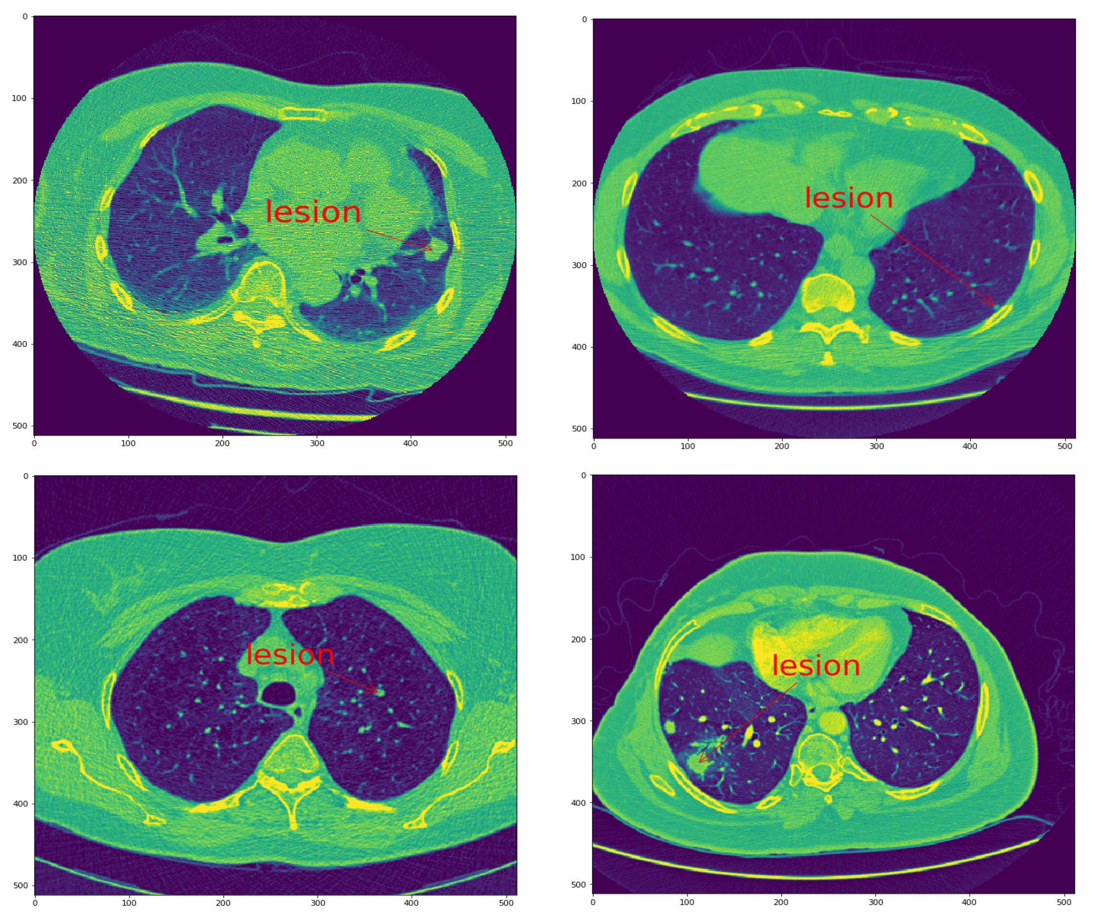
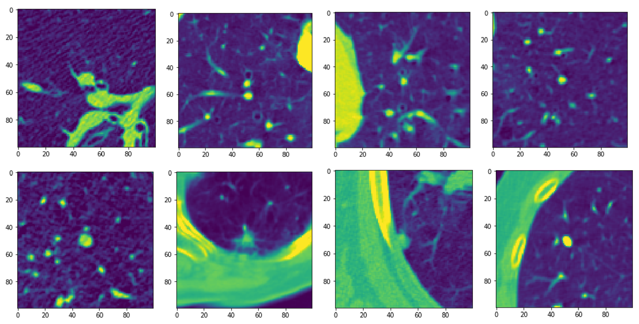
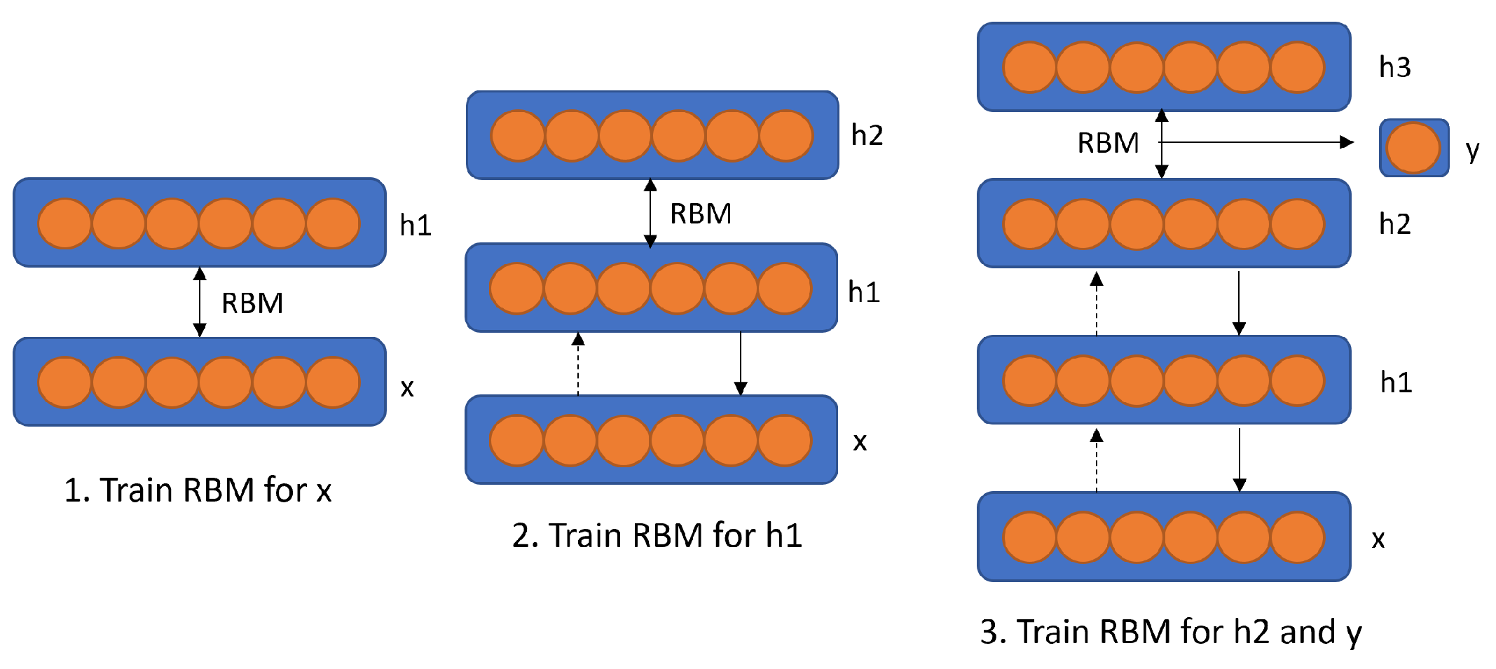
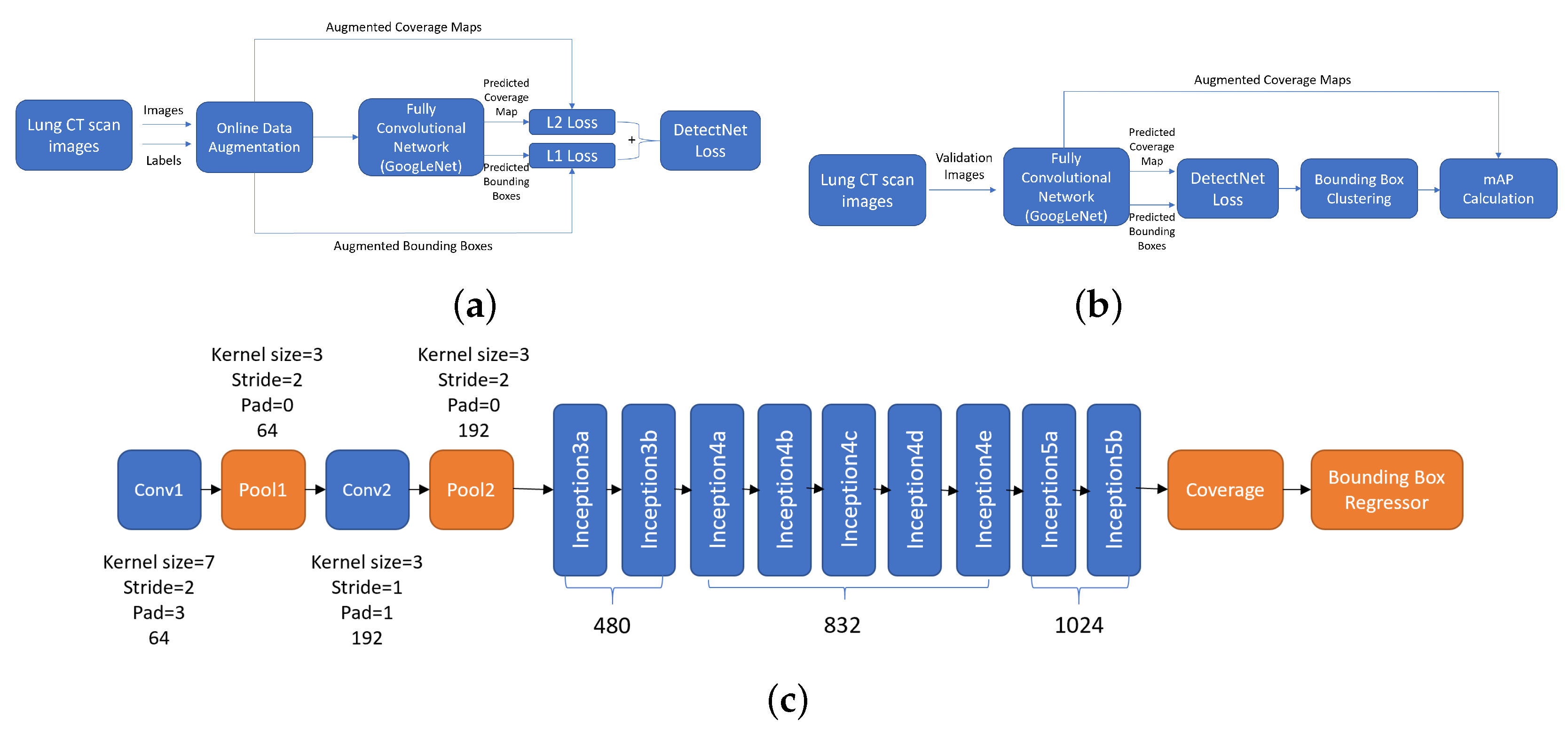
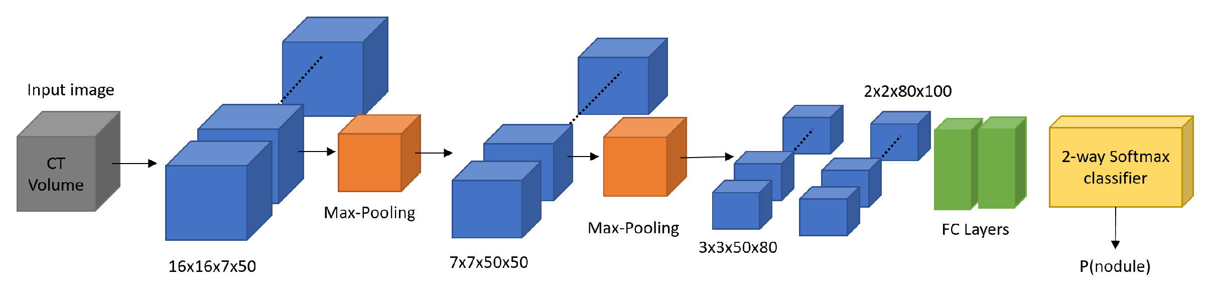
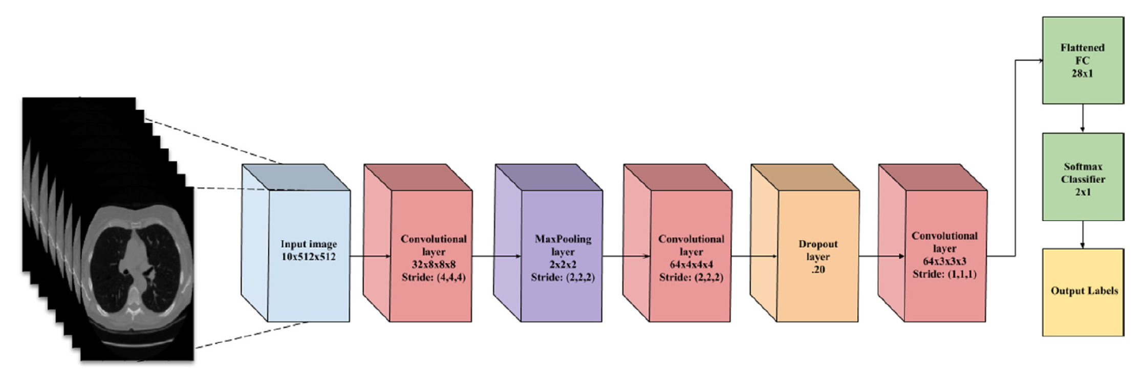
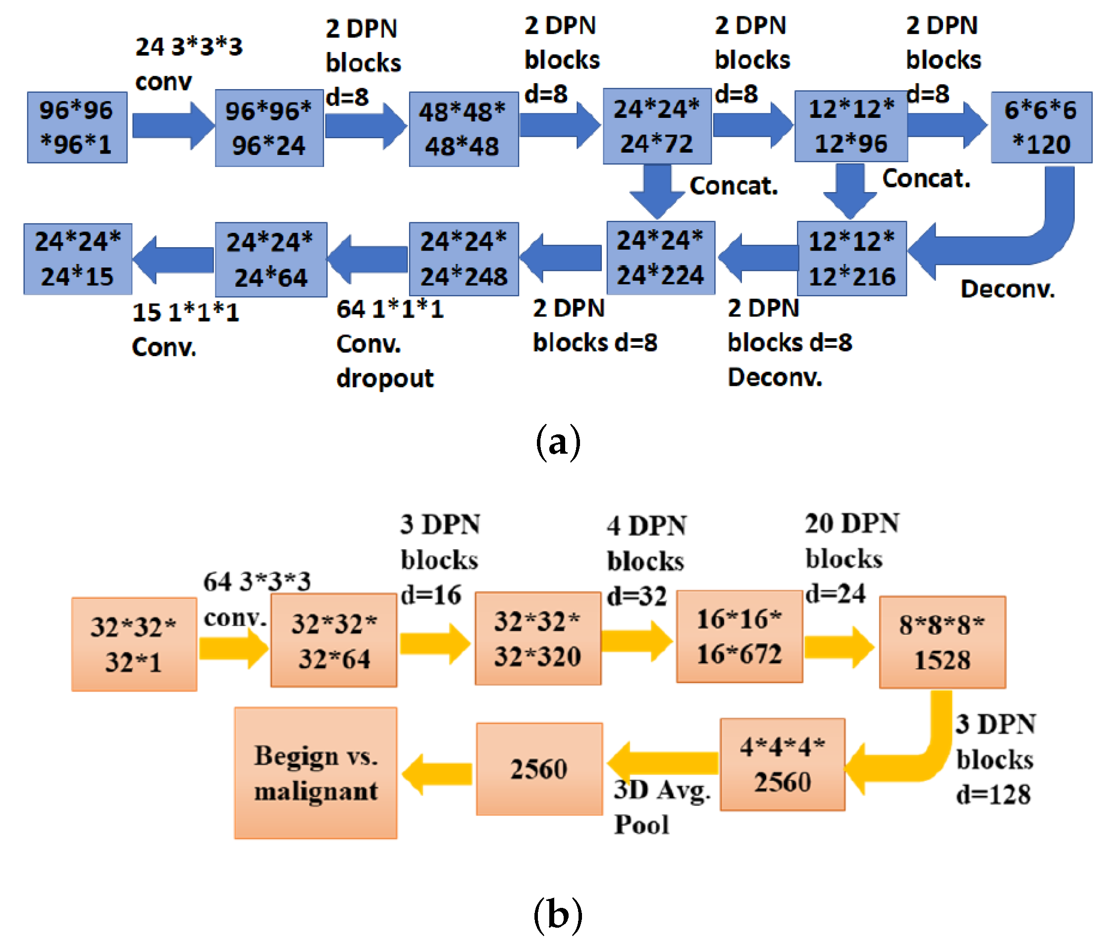
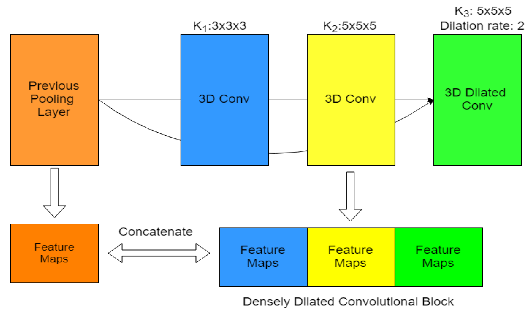
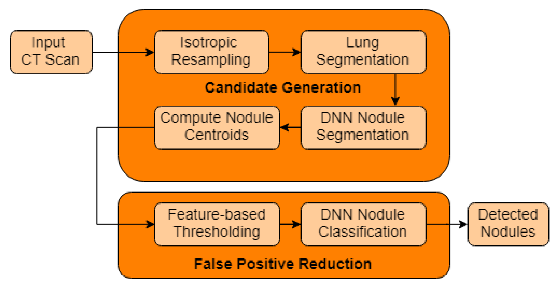
Table 1.
CT Scans datasets for lung cancer detection (* shows the datasets that have associated nodule annotations).
Table 1.
CT Scans datasets for lung cancer detection (* shows the datasets that have associated nodule annotations).
| Dataset | Number of CT Scans | Annotations |
|---|---|---|
| LIDC-IDRI [17] | 1018 | * |
| LUNA16 [19] | 888 | * |
| SPIE-AAPM-NCI [20] | 70 | * |
| NLST [1] | 3410 | * |
| ANODE09 [21] | 55 | * |
| DLCST [23] | 612 | * |
| DSB [25] | 1902 | - |
Table 2.
Metrics used in deep learning lung cancer detection literature.
| Metric | Definition | Note |
|---|---|---|
| Sensitivity | True positive rate (TPR) or recall | |
| Specificity | True negative rate (TNR) | |
| Accuracy | Total true results | |
| Precision | Positive predicted value (PPV) | |
| F1-Score | Relates the sensitivity and precision measures | |
| ROC | Curve depicting the relationship between the sensitivity and specificity (Y-axis is the true positive rate and the X-axis is the false positive rate) | Receiver Operating Characteristic (ROC) curve |
| FROC | Similar to the ROC curve, differing only in the X-axis. The X-axis is the false positive rate per image (or per scan) | Free Response Operating Characteristic (ROC) curve |
| AUC | Total area under the ROC curve | Area Under Curve (AUC) |
| CPM | Average of the sensitivity at seven defined false positive rates in the FROC curve: , , , 1, 2, 4 and 8 FPs/scan | Competition Performance Metric (CPM) |
= True Positives; = True Negatives; = False Positives; = False Negatives.
Table 3.
Measured performance of the three different models.
| Models | Accuracy % | Sensitivity % | Specificity % | AUC |
|---|---|---|---|---|
| 2D CNN slice-level | 86.7% | 78.6% | 91.2% | 0.926 ± 0.014 |
| 2D CNN nodule-level | 87.3% | 88.5% | 86.0% | 0.937 ± 0.014 |
| 3D CNN | 87.4% | 89.4% | 85.2% | 0.947 ± 0.014 |
Table 4.
Performance at 1/8, 1/4, 1/2, 1, 2, 4, 8 FPs/scan.
| FPs/scan | 0.125 | 0.25 | 0.5 | 1 | 2 | 4 | 8 | Average |
| DNs | 1056 | 1104 | 1120 | 1126 | 1144 | 1153 | 1158 | 1123 |
| Sensitivity | 0.890 | 0.931 | 0.944 | 0.949 | 0.965 | 0.972 | 0.976 | 0.947 |
| FNR | 0.110 | 0.069 | 0.056 | 0.051 | 0.035 | 0.028 | 0.024 | 0.053 |
Table 5.
Results obtained in Reference [78].
Table 5.
Results obtained in Reference [78].
| Task | Sensitivity | FPPS | ROC AUC |
|---|---|---|---|
| CG | 0.9477 | 30.39 | - |
| FPR | 0.9421 | 1.789 | 0.9835 |
| Complete system | 0.8929 | 1.789 | 0.9324 |
Table 6.
Results of the Architecture on LUNA16 as in Reference [89].
Table 6.
Results of the Architecture on LUNA16 as in Reference [89].
| FPs per scan | 0.125 | 0.25 | 0.5 | 1 | 2 | 4 | 8 |
| Sensitivity (%) | 81.7 | 85.1 | 86.9 | 88.3 | 89.1 | 90.7 | 91.4 |
Table 7.
Performance benchmark of the multi-view CNN configurations on LUNA16 as in Reference [94].
Table 7.
Performance benchmark of the multi-view CNN configurations on LUNA16 as in Reference [94].
| Configuration | Number of Views | AUC | CPM |
|---|---|---|---|
| Combined Algorithms | - | 0.969 | 0.573 |
| Single-view | 1 | 0.969 | 0.481 |
| Committee-fusion | 3 | 0.981 | 0.696 |
| 9 | 0.987 | 0.780 | |
| Late-fusion | 3 | 0.987 | 0.742 |
| 9 | 0.993 | 0.827 | |
| Mixed-fusion | 3×3 | 0.996 | 0.824 |
Table 8.
Comparative results of candidate detection models.
| Ref. | Database | SE % | FPs/scan | CPM | PPV | Architecture | Approach |
|---|---|---|---|---|---|---|---|
| [49] | LUNA16 | 94.6 | 15 | CNN | 2D | ||
| [42] | LUNA16 | 86.42 | 0.775 | CNN | 2D | ||
| [52] | LIDC | 80/95 | 22.4/563 | CCN | 3D | ||
| [78] | LUNA16 | 94.77 | 30.39 | CNN | 3D | ||
| [82] | LUNA16 | 99.1 | 0.059 | CNN | 3D | ||
| [82] | LUNA16 | 0.951 | CNN | 3D | |||
| [82] | LUNA16 | 0.95 | CNN | 3D |
Table 9.
Comparative results of false positive reduction models.
| Ref. | Database | SE % | FPs/scan | ACC % | CPM | AUC | Architecture | Approach |
|---|---|---|---|---|---|---|---|---|
| [42] | LUNA16 | 73.4/74.4 | 0.125/0.25 | 0.79 | 0.954 | CNN | 2D | |
| [92] | LIDC | 96 | MSAE/CNN | 2D | ||||
| [94] | LUNA16 | 85.4/90.1 | 1.0/4.0 | 0.824 | 0.996 | CNN | 2D | |
| [94] | ANODE09 | 0.637 | CNN | 2D | ||||
| [94] | DLCST | 76.5 | 6 | CNN | 2D | |||
| [49] | LUNA16 | 92.2/94.4 | 1.0/4.0 | 0.891 | CNN | 3D | ||
| [52] | LIDC | 80 | 15.28 | CNN | 3D | |||
| [78] | LUNA16 | 94.21 | 1.789 | 0.983 | CNN | 3D | ||
| [82] | LUNA16 | 0.966 | CNN | 3D | ||||
| [82] | LUNA16 | 0.968 | CNN | 3D | ||||
| [82] | LUNA16 | 0.916 | CNN | 3D | ||||
| [99] | LUNA16 | 92.2 | 8 | 0.827 | CNN | 3D | ||
| [100] | LUNA16/LIDC | 88.83 | CNN | 3D |
Table 10.
Comparative results of the different proposed nodule detection models
| Ref. | Database | SP % | SE % | FPs/scan | ACC % | CPM | AUC | PPV | Architecture | Approach |
|---|---|---|---|---|---|---|---|---|---|---|
| [31] | LIDC | 83.25 | 0.39 | Autoencoder | 2D | |||||
| [33] | LIDC | 82.2 | 73.4 | DBN | 2D | |||||
| [33] | LIDC | 78.7 | 73.3 | CNN | 2D | |||||
| [54] | LIDC | 86 | 88.5 | 87.3 | 0.937 | CNN | 2D | |||
| [35] | LIDC | 79.76 | CNN | 2D | ||||||
| [35] | LIDC | 81.19 | DBN | 2D | ||||||
| [35] | LIDC | 79.29 | SDAE | 2D | ||||||
| [37] | LIDC | 89 | 6 | 0.93 | CNN | 2D | ||||
| [40] | LHMC/UCM/NLST/DBS1&2 | 0.87/0.83/0.88/0.82/0.84 | CNN | 2D | ||||||
| [41] | LIDC | 92.02 | 84.19 | 89.53 | 0.9665 | Fuse-TSD | 2D | |||
| [27] | LIDC | 60/66/73/76/77 | 0.125/0.25/1/2/4 | 0.71 | CNN | 2D | ||||
| [92] | LIDC | 96 | MSAE/CNN | 2D | ||||||
| [94] | LUNA16 | 85.4/90.1 | 1/4 | 0.824 | 0.996 | CNN | 2D | |||
| [94] | ANODE09 | 0.637 | CNN | 2D | ||||||
| [94] | DLCST | 76.5 | 6 | CNN | 2D | |||||
| [46] | AAPM-SPIE | 80 | 10 | CNN | 3D | |||||
| [48] | LIDC | 78.9/71.2 | 20/10 | CNN | 3D | |||||
| [54] | LIDC | 85.2 | 89.4 | 87.4 | 0.947 | CNN | 3D | |||
| [55] | LIDC | 93 | 77 | 87.14 | 0.93 | MC-CNN | 3D | |||
| [58] | LIDC | 90 | 5 | CNN | 3D | |||||
| [64] | LUNA16 | 90.6 | 2 | 0.839 | FCN/CNN | 3D | ||||
| [66] | DBS | 81.42 | 0.8562 | 0.87 | CNN | 3D | ||||
| [68] | LUNA16 | 55.3 | 58.9 | 64.4 | 0.542 | CNN | 3D | |||
| [69] | LIDC | 81.41 | DPN | 3D | ||||||
| [74] | LUNA16 | 89.0/93.1/94.9/96.5/97.2 | 0.125/0.25/1/2/4 | 0.947 | CNN | 3D | ||||
| [77] | LIDC | 90.4 | 48.6 | 88.8 | CNN | 3D | ||||
| [78] | LUNA16 | 89.29 | 1.789 | 0.8135 | 0.9324 | CNN | 3D | |||
| [82] | LUNA16 | 0.947 | CNN | 3D | ||||||
| [99] | LUNA16 | 92.2 | 8 | 0.827 | CNN | 3D | ||||
| [89] | LUNA16/Ali Tianchi | 81.7/85.1/88.3/89.1/90.7 | 0.125/0.25/1/2/4 | 0.876 | CNN | 3D | ||||
| [85] | NLST | 0.949 | CNN | 3D |
© 2020 by the authors. Licensee MDPI, Basel, Switzerland. This article is an open access article distributed under the terms and conditions of the Creative Commons Attribution (CC BY) license (http://creativecommons.org/licenses/by/4.0/).
Share and Cite
MDPI and ACS Style
Riquelme, D.; Akhloufi, M.A. Deep Learning for Lung Cancer Nodules Detection and Classification in CT Scans. AI 2020, 1, 28-67. https://doi.org/10.3390/ai1010003
AMA Style
Riquelme D, Akhloufi MA. Deep Learning for Lung Cancer Nodules Detection and Classification in CT Scans. AI. 2020; 1(1):28-67. https://doi.org/10.3390/ai1010003
Chicago/Turabian StyleRiquelme, Diego, and Moulay A. Akhloufi. 2020. "Deep Learning for Lung Cancer Nodules Detection and Classification in CT Scans" AI 1, no. 1: 28-67. https://doi.org/10.3390/ai1010003