
Subsurface Lateral Solute Transport in Turfgrass
by
 ,
,
Manuel E. Camacho
1,2,
Carlos A. Faúndez-Urbina
3,
Aziz Amoozegar
1,
Travis W. Gannon
1,
Joshua L. Heitman
1 and
Ramon G. Leon
1,* 1
Department of Crop and Soil Sciences, North Carolina State University, Campus Box 7620, Raleigh, NC 27695, USA
2
Escuela de Agronomía (EA) y Centro de Investigaciones Agronómicas (CIA), Universidad de Costa Rica, San Pedro 11503-2060, Costa Rica
3
Núcleo de Investigaciones Aplicadas en Ciencias Veterinarias y Agronómicas, Universidad de Las Américas, Avenida Manuel Montt 948, Santiago 7500975, Chile
*
Author to whom correspondence should be addressed.
Agronomy 2023, 13(3), 903; https://doi.org/10.3390/agronomy13030903
Submission received: 26 February 2023
/
Revised: 14 March 2023
/
Accepted: 16 March 2023
/
Published: 18 March 2023
(This article belongs to the Section Grassland and Pasture Science)
Abstract
:Turfgrass managers have suspected that runoff-independent movement of herbicides and fertilizers is partially responsible for uneven turfgrass quality in sloped areas. We hypothesized that subsurface lateral solute transport might explain this phenomenon especially in areas with abrupt textural changes between surface and subsurface horizons. A study was conducted to track solute transport using bromide (Br−), a conservative tracer, as a proxy of turfgrass soil inputs. Field data confirmed the subsurface lateral movement of Br− following the soil slope direction, which advanced along the boundary between soil horizons over time. A model based on field data indicated that subsurface lateral movement is a mechanism that can transport fertilizers and herbicides away from the application area after they have been incorporated within the soil, and those solutes could accumulate and resurface downslope. Our results demonstrate that subsurface lateral transport of solutes, commonly ignored in risk assessment, can be an important process for off-target movement of fertilizers and pesticides within soils and turfgrass systems in sloped urban and recreational landscapes.
1. Introduction
The use of chemicals, such as fertilizers, herbicides, and other pesticides, has become a fundamental tool for growing plants in agricultural and non-agricultural systems [1]. However, there are concerns about the risk of transport of these chemicals from agricultural, recreational, and urban sites (non-point sources) to terrestrial and aquatic systems where they can cause health, economic, and environmental problems [2,3]. Off-target movement of herbicides/pesticides and fertilizers occurs in diverse forms such as drift, leaching through soil, and surface runoff. Of these, surface runoff has been reported as one of the main pathways by which these chemicals move away from application areas [2,4]. For instance, in turfgrass, herbicides with differing water solubility and soil adsorption affinity exhibited runoff movement along the soil surface, and this runoff increased under sloped conditions and heavy rainfall events [5].
Turfgrass managers have reported herbicide injury at the bottom of sloped turfgrass landscapes, but the injury pattern did not match runoff transport of the herbicide from the original application area [6]. A possible explanation is the transport of dissolved chemicals (including herbicides) through subsurface lateral flow [7,8], which is more likely to occur in hillslope soils, allowing solute displacement from upslope and accumulation in downslope areas.
Subsurface lateral flow has been reported in forestry, perennial systems, and catchments [9,10,11,12], and it is more likely to occur in soils with distinct soil horizon boundaries due to substantial change in the hydraulic properties of the two layers [9,13,14]. However, the mechanisms of subsurface lateral flow and its role on herbicides/fertilizer movement have not been described in turfgrass landscapes where its consequences are easily detected with changes in turfgrass quality, especially when phytotoxicity occurs due to herbicide accumulation. Furthermore, turfgrass is an important component of managed vegetation systems in urban (e.g., home lawn) and recreational (e.g., golf course) sites, representing the largest acreage of any irrigated crop in the US [15]. In addition, due to the extensive use of lawns in urban landscapes in highly populated areas, there is more interest in understanding the impact of this crop on natural resources [16,17].
Studies of subsurface lateral water flow in soils are scarce, and even scarcer are those with texture-contrast soils under slope conditions. Hardie et al. [7] described that lateral water movement is likely to occur in soils with texture contrast in the vertical direction as a consequence of hydraulic discontinuity among A and B horizons. However, they pointed out that these lateral transport mechanisms were unclear, and further field research should be conducted. Furthermore, the mechanisms described by Hardie et al. [7] were uncharted for layered soils under sloped conditions.
The main goal of the present study was to determine whether subsurface lateral movement is a mechanism that could explain solute off-target movement in turfgrass. Thus, the objectives were to: (1) investigate the potential subsurface lateral movement of solutes in a sloped soil with divergent surface and subsurface soil textures, and (2) develop a model to characterize the mechanics of lateral subsurface solute movement under conditions generally present in turfgrass.
2. Materials and Methods
2.1. Field Experiment
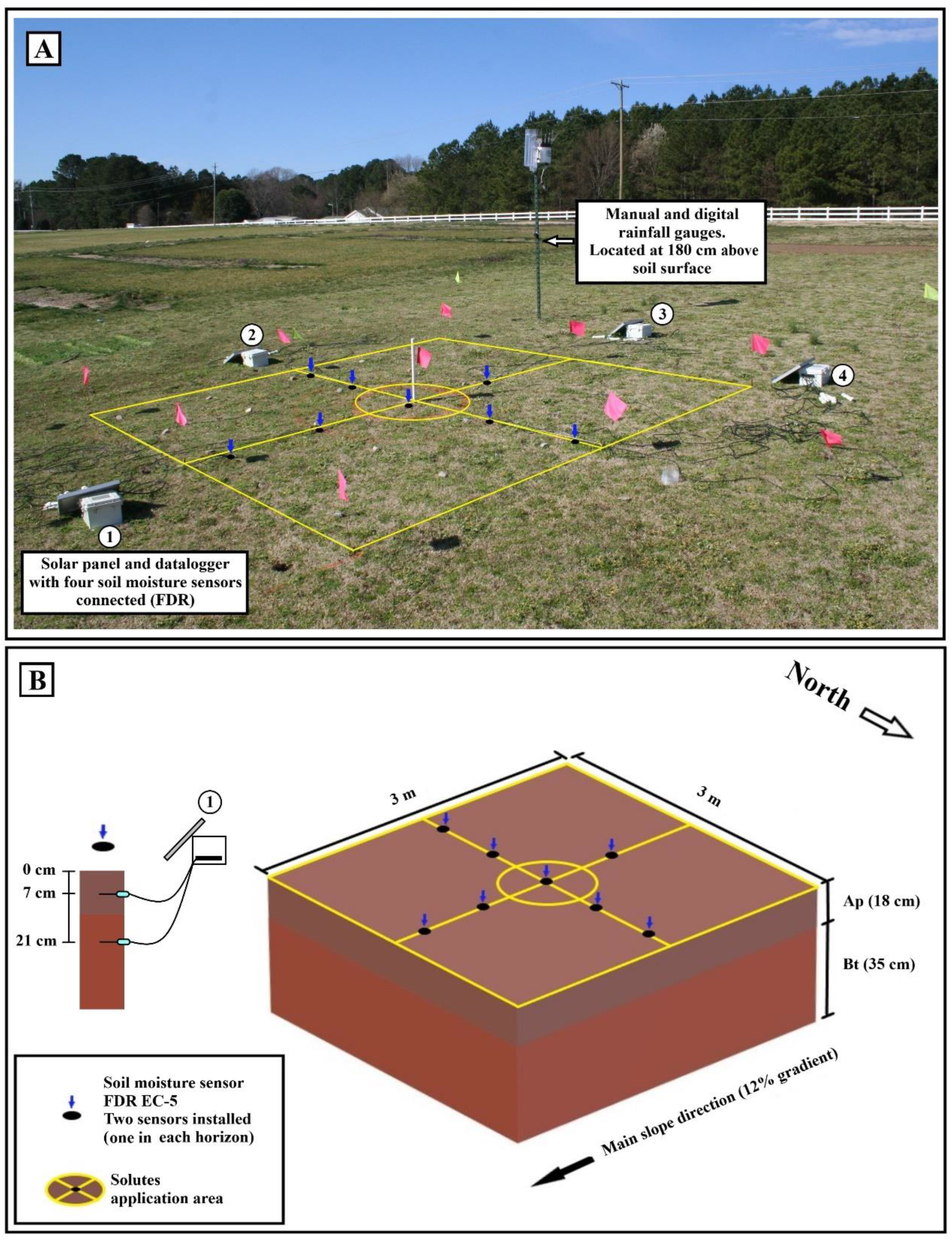
A field experiment was conducted between the months of January and April, 2021 at the Lake Wheeler Turf Field Laboratory at North Carolina State University in Raleigh, NC. The experiment was conducted during the winter season, with several rainfall events (>1 cm) during February and March. The soil in the field is a Cecil sandy loam (fine, kaolinitic, thermic Typic Kanhapludult). The Ap horizon (sand texture) is on average 0.18 m thick, overlaying the Bt horizon (clay texture) that is more than 0.35 m thick (Table 1). The plot and the surrounding area have 12% slope covered with hybrid bermudagrass [Cynodon dactylon (L.) Pers. × Cynodon transvaalensis Burtt-Davey ‘Tifway 419’], which was dormant at the time of the experiment. A 3 × 3 m area, established as the experimental area, was divided into four equal sections (Figure 1). The sides of the four sections were marked with nylon strings as guides for installing water content monitoring sensors and collecting samples for solute transport assessment.
2.2. Soil Sampling and Laboratory Analysis
Using 7.62 cm diameter and 7.62 cm long aluminum cylinders (347.5 cm3) in an Uhland soil sampler [18], undisturbed soil cores were collected from two depth intervals in the Ap and the upper part of the Bt horizon at six different locations surrounding the experimental area. The soil cores were trimmed in the field and transported to the laboratory for analysis. The intact soil cores were divided into two groups, one used to quantify saturated hydraulic conductivity (Ks) and the other for soil water retention analysis after slowly saturating them from the bottom over a 24-h period. In addition, three bulk samples were collected from each soil horizon and used for particle size distribution analysis using the hydrometer method [19].
Saturated hydraulic conductivity of the undisturbed soil cores (from the first group) was measured using the constant head method [20], and intact soil cores (from the second group) were used to generate water retention curves [21]. Water retention was determined separately for high-water potential (0 to −0.032 MPa) and low-water potential (−0.1 to −1.5 MPa). After reaching equilibrium for each pressure, bulk density and final water content were determined [22,23]. For low soil water potential, the analysis was carried out using disturbed soil samples, porous plates, and pressure vessels (Soil Moisture Equipment Corp., Santa Barbara, CA, USA) [24].
2.3. Weather and Soil Water Content Monitoring
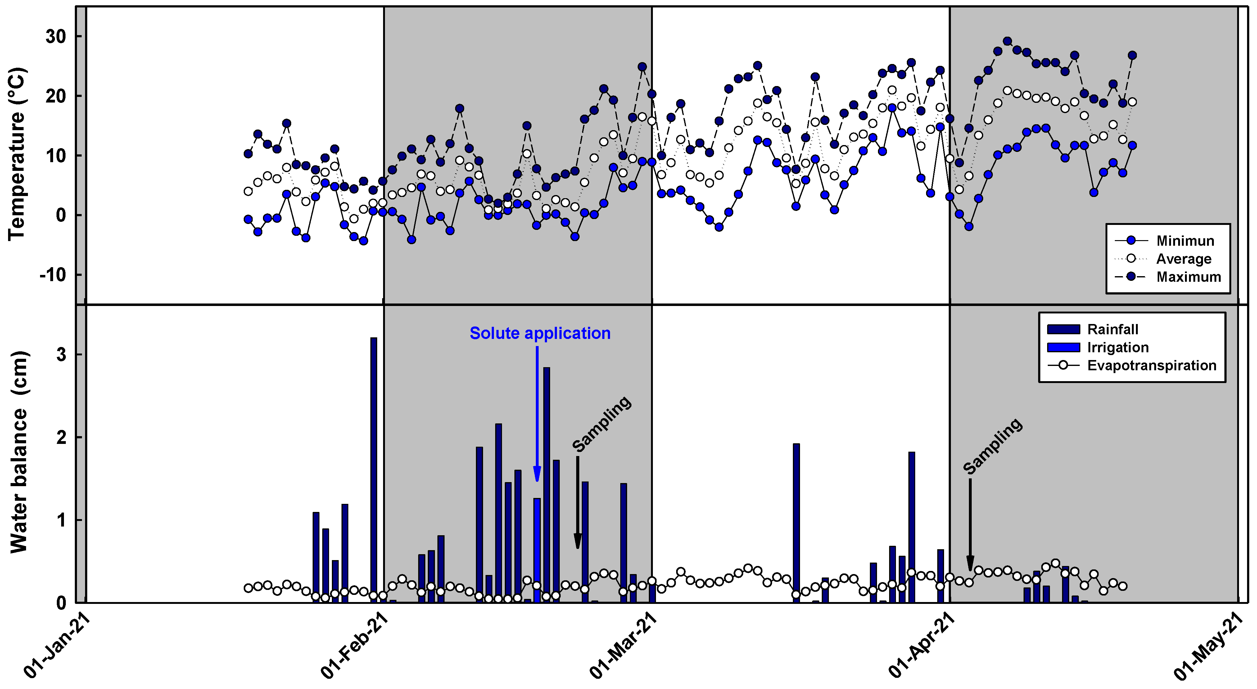
Two rain gauges, one manual (Stratus® RG-202, RainmanWeather, Jacksonville, FL, USA, with 0.25 mm resolution), and another digital (Onset® RG3-M Bourne, MA, USA, with a resolution of 0.20 mm) were installed at 180 cm above the ground close to the experimental plot (Figure 1A) to monitor rainfall. Soil water content was monitored every 15 min at an average depth of 7 cm (Ap horizon) and 21 cm (top part of Bt horizon) using EC-5 frequency domain reflectometry (FDR) soil moisture sensors (Onset Computer Corporation ® Bourne, MA, USA) with a reading resolution of 0.001 cm3 cm−3 and accuracy of ±0.03 cm3 cm−3. Eight monitoring points were established in a concentric arrangement (Figure 1B). At each monitoring location, an auger hole (7.5 cm diameter, 0 to 40 cm depth) was dug for horizontally installing the two soil moisture sensors into each soil horizon (Figure 1B). These sensors were connected to HOBO U30 data loggers (Onset Computer Corporation®, Bourne, MA, USA). The auger holes were backfilled with the original soil and then allowed to settle for one month prior to the initiation of the experiment. In addition to site monitoring, daily minimum and maximum temperature, precipitation, and potential evapotranspiration (ETp, estimated using Penman-Monteith model) (Figure 2) were obtained from an ECONET automated weather station (North Carolina State Climate Office, NC, USA) located within 1 km of the experimental site.
2.4. Solute Application and Post Irrigation Treatment
Bromide (Br−) was selected as indicator of solute movement as a proxy for herbicides and fertilizers. As a conservative tracer, Br− does not bind to soil particles, allowing to describe solute movement in the soil more easily and in shorter periods of time. Furthermore, it prevents the confounding effects associated with chemical changes and soil microbial degradation of more complex molecules. Solute application was conducted on 17 February 2021 following three consecutive rainfall events (>1.5 cm) under low evapotranspiration conditions (Figure 2). This date was selected with the intent that soil conditions were near saturation at the boundary between the Ap and Bt horizons. Measured soil water content values at the application date were 0.33 and 0.41 cm3 cm−3 for the Ap and Bt horizons, respectively. One liter of potassium bromide (KBr 99+%, Thermo Scientific Chemicals, Waltham, MA, USA) solution, at a concentration of 1.52 mol L−1, was uniformly applied by hand to a 0.38-m2 circular area at the center of the plot (Figure 1). The solute was applied using a CO2 pressurized backpack sprayer with a flat-fan spray nozzle (XR11002VS, TeeJet®, Spraying Systems Co., Wheaton, IL, USA). This equipment was calibrated to deliver 280 L ha−1 of solution at 12.3 mL sec−1. Three hours after the solute application, the entire experimental area was irrigated with 1.26 cm of water in three events (114 L of water split into three applications: 49, 46, and 19 L) that were spaced one hour apart to allow the KBr solution to infiltrate into the soil. This amount of irrigation was chosen to supplement rainfall events and ensure soil saturation at the boundary between Ap and Bt horizons while avoiding surface runoff. Irrigation was carried out using a hose coupled with a wand with an electronic flow meter (GPI® 01N31GM, Great Plains Industries Inc., Wichita, KS, USA). Irrigation was withheld for the rest of the experiment period.
2.5. Soil Sampling for Br− Extraction and Measurement
Soil samples were collected at 5 and 46 days after the solute application (DASA). These dates were selected based on the amount and distribution of the rainfall received after the application to allow enough time to detect Br− movement through the soil (Figure 2). Samples were systematically collected in a 60 × 60 cm grid to characterize lateral movement of the solutes within the whole experimental area. This grid sampling system was designed to include a central transect (3 m length) that encompassed the solute application area and sampling points up- and downslope following the main slope direction. Soil samples were taken as described in Table 2. The second sampling presented finer depth increments in the Ap to increase the resolution for Br− recovery and analysis to account for any potential dilution and solute loss.
Bromide quantification was performed by mixing 120 g of soil of each sample with 240 mL of deionized water in a mason jar (473 mL capacity) and vigorously shaken for 30 min using a reciprocal shaker (Eberbach Corporation®, MI, USA) at 240 oscillations min−1. The samples were allowed to settle overnight, and the supernatant was filtered using Whatman No. 42 filter paper. Bromide concentration was measured using an Oakton® pH 450 (pH/mV meter, Thermo Fisher Scientific, Waltham, MA, USA) and a Cole-Parmer® combination Ion-Selective Electrode (ISE, Cole-Parmer, Vernon Hills, IL, USA) [25].
2.6. HYDRUS-2D Modelling
HYDRUS-2D software package was used to simulate the lateral water flow and solute movement for soil conditions mimicking the field experiment [26,27]. The two-dimensional variably saturated flow was solved numerically via the Galerkin finite element method using the Richards equation [28]. Bromide transport was predicted employing the advection-dispersion equation (ADE) using transversal and longitudinal dispersivity (L) and molecular diffusion into the water phase (L2 T−1) [28]. This was performed under the assumption of isotropic conditions within each soil horizon.
Unsaturated soil hydraulic conductivity (Kh) and the volumetric soil water content (θh) as functions of soil water pressure head (h) (i.e., matric potential expressed on weight basis) were fitted for each soil horizon using the van Genuchten model [29]:
where θs and θr are the saturated and residual water contents (L3 L−3), respectively; Ks is saturated hydraulic conductivity (L T−1); α (L−1) and n (dimensionless) are empirical fitting parameters; m is related to n by m = 1 − 1/n; l is an empirical pore-connectivity parameter (fixed at 0.5); and Se is the dimensionless soil effective saturation. The parameters θs, θr, α, and n were fitted from the soil water retention data generated as described above through nonlinear least-squares optimization with the RETC program [30]. The same parameters were used together with measured Ks to estimate Kh using Equation (2). For the Bt horizon, a 2 cm air entry pressure was assigned as recommended for fine-textured soils [31].
For Br−, we used 10.0 and 1.0 cm as longitudinal and transversal dispersivity, respectively [28], and a molecular diffusion coefficient in free water of 1.6 cm2 d−1. We did not include Kd for bromide, an anion, because it is considered a non-reactive (i.e., non-adsorbing), conservative tracer with low risk of attenuation by soil [32,33].
Soil Domain, Initial and Boundary Conditions, and Numerical Implementation
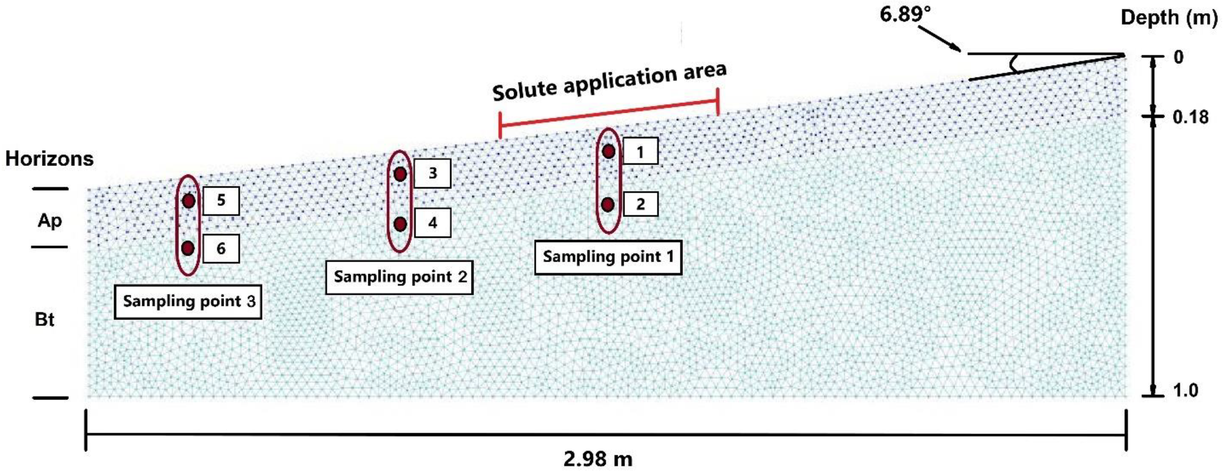
The soil 2D domain was represented in the model by a finite element grid, composed of 8147 non-uniform triangular elements and 4202 nodes. The mesh was refined around the surface to produce a relatively fine grid pattern for the Ap horizon and a relatively coarse grid pattern for the Bt horizon, including a slope angle of 6.89° (i.e., 12%) (Figure 3).
Two initial conditions (IC) for pressure head corresponding to the two soil horizons were set in the model. The Ap horizon had a linear distribution with depth and slope in the x-direction with top and bottom pressure head iCs of −780 and −400 cm, respectively. The Bt horizon had a linear distribution with depth and 12% slope in the x-direction with top and bottom pressure head iCs of −400 and −333 cm, respectively. These values were chosen based on the initial soil water content obtained from the FDR sensors and their corresponding pressure head from the measured water retention curve. The initial concentration of the solutes in the soil was set as 0 mg cm−3, and the solute pulse concentration after application was calculated using the following equation:
where ϑ is a reduction factor (between 0 and 1) for ETp measured at the weather station (aiming to adjust this ETp to just evaporation, assuming no transpiration due to plant dormancy), I is irrigation, and R is rainfall obtained for the application day (a). A time-variable flux boundary condition was assigned to a 70 cm diameter circle (3848 cm2) in the center of the experimental plot (Figure 3). This variable flux was estimated for each day i using the following equation:
An atmospheric boundary condition was assigned to the rest of the soil surface (115 cm downslope and 115 cm upslope), where HYDRUS 2D performed the corresponding calculations automatically using rainfall and evaporation. A free drainage boundary condition was applied to the bottom of the soil domain, and no-flow boundary condition was established along the vertical upslope edge of the domain. For the vertical downslope edge, a gradient boundary condition was assigned. This is a special boundary condition available in HYDRUS, which can be used for flow simulations under hill slope conditions where the side-gradient is almost parallel with the slope’s main direction. We used a factor of 0.12, which was calculated using the following equation:
where grad is the gradient factor, and α is the soil slope angle (6.89° = 0.12π for this case).
For solute transport, a third-type boundary condition (Cauchy) was assigned to the top and the bottom of the domain. For the application area, we assigned an independent third-type boundary condition to maintain the variable flux boundary conditions for this region [34].
All simulations were performed considering a period of 80 days, aiming to cover: (1) all the rainfall events since the soil moisture sensors were installed at day 1 (t0), (2) the solute application 30 days after t0, (3) the two sampling dates after solute application, and (4) to have sufficient data aiming to perform long-term simulations.
2.7. Statistical Analysis
The model performance was evaluated with the root mean square error (RMSE), the Willmott agreement index (d), and the Nash-Sutcliffe efficiency (NSE) index. All these indices were calculated using the package “ie2misc” in R Studio (R v. 4.0.4, 2021-02-15) “Lost Library Book” [35].
The Br− distribution within the plot graphs (contour maps) were produced using contour plot option of SigmaPlot 11.0 software (Systat Software Inc., Chicago, IL, USA), which performs a bicubic interpolation between the data points.
3. Results
3.1. Field Observations
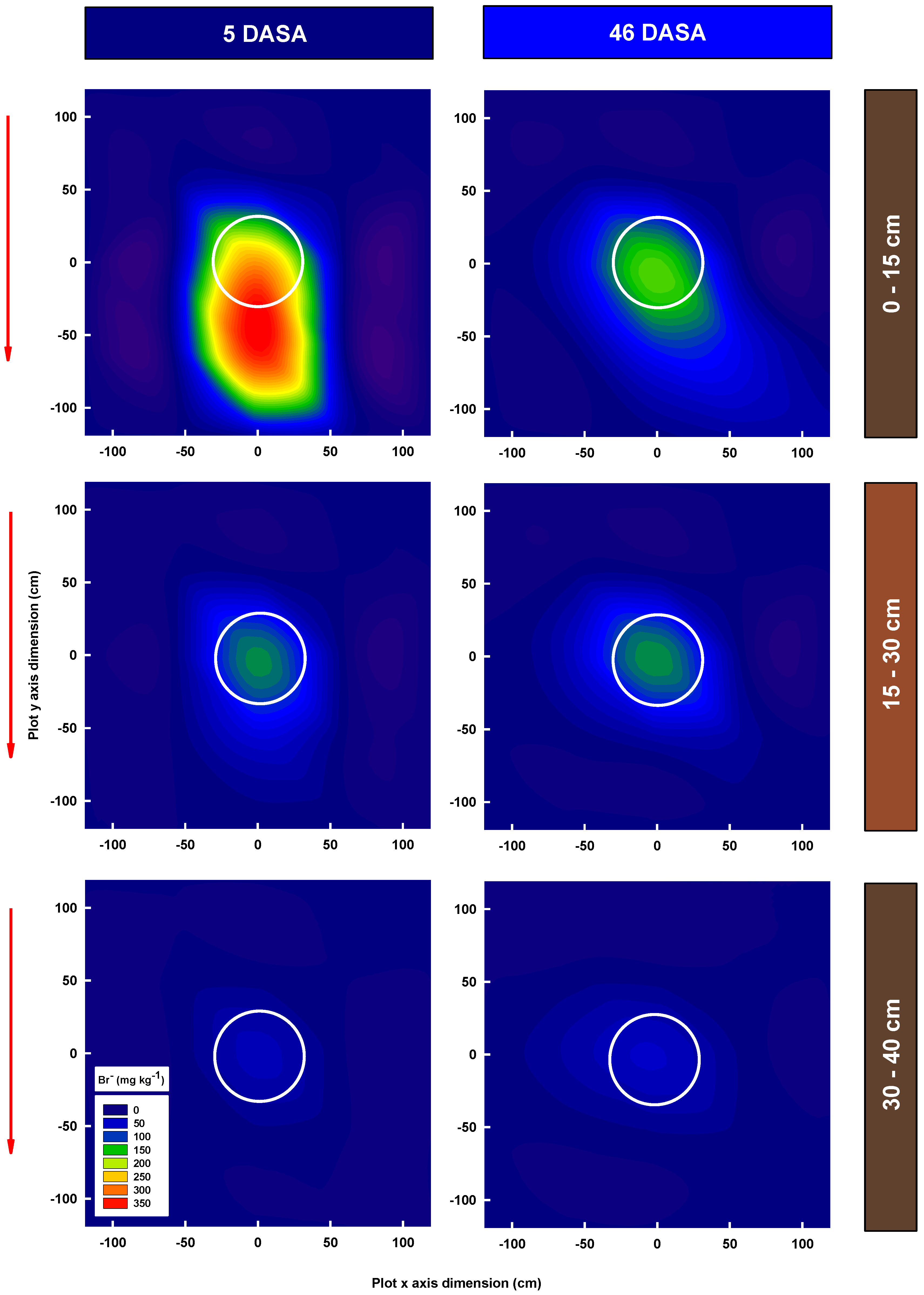
In both evaluation dates (5 and 46 DASA), Br− concentrations decreased with soil depth (Figure 4), but 5 DASA, Br− moved laterally downslope forming a plume, around 90 cm away from the application area (central white circle). This movement was more evident in the top 15 cm of the soil profile (Ap horizon), but a similar pattern was also observed within 15–30 cm depth.
When assessing the Br− distribution 46 DASA, a pattern of lateral movement similar to 5 DASA was observed at 0–15 cm depth with considerably lower concentrations (due to solute dilution). The plume continued moving along the main slope direction with a slight angle towards the North-East. Although Br− moved vertically within the soil and the concentration increased within 15–30 and 30–40 cm depths compared with 5 DASA, lateral movement was predominantly along the slope.
3.2. Modeling Results and Comparison with Measured Data
Results obtained with HYDRUS 2D for Br− concentration and soil water content dynamics were more accurate for the latter than for the former (Table 3). For example, the RMSE for Br− concentration was higher than 0.4 mg cm−3, and the Willmott agreement index (d) obtained was lower than 0.5. Conversely, the volumetric soil water content values obtained with HYDRUS 2D were closer to corresponding measured data in both soil horizons and sampling points assessed. This model presented an excellent performance predicting the water content dynamics in both soil horizons, with the RMSE was lower than 0.030 m3 m−3, and the Willmot agreement (d) and Nash-Sutcliffe efficiency (NSE) were higher than 0.8.
3.3. Spatial and Temporal Solute Movement
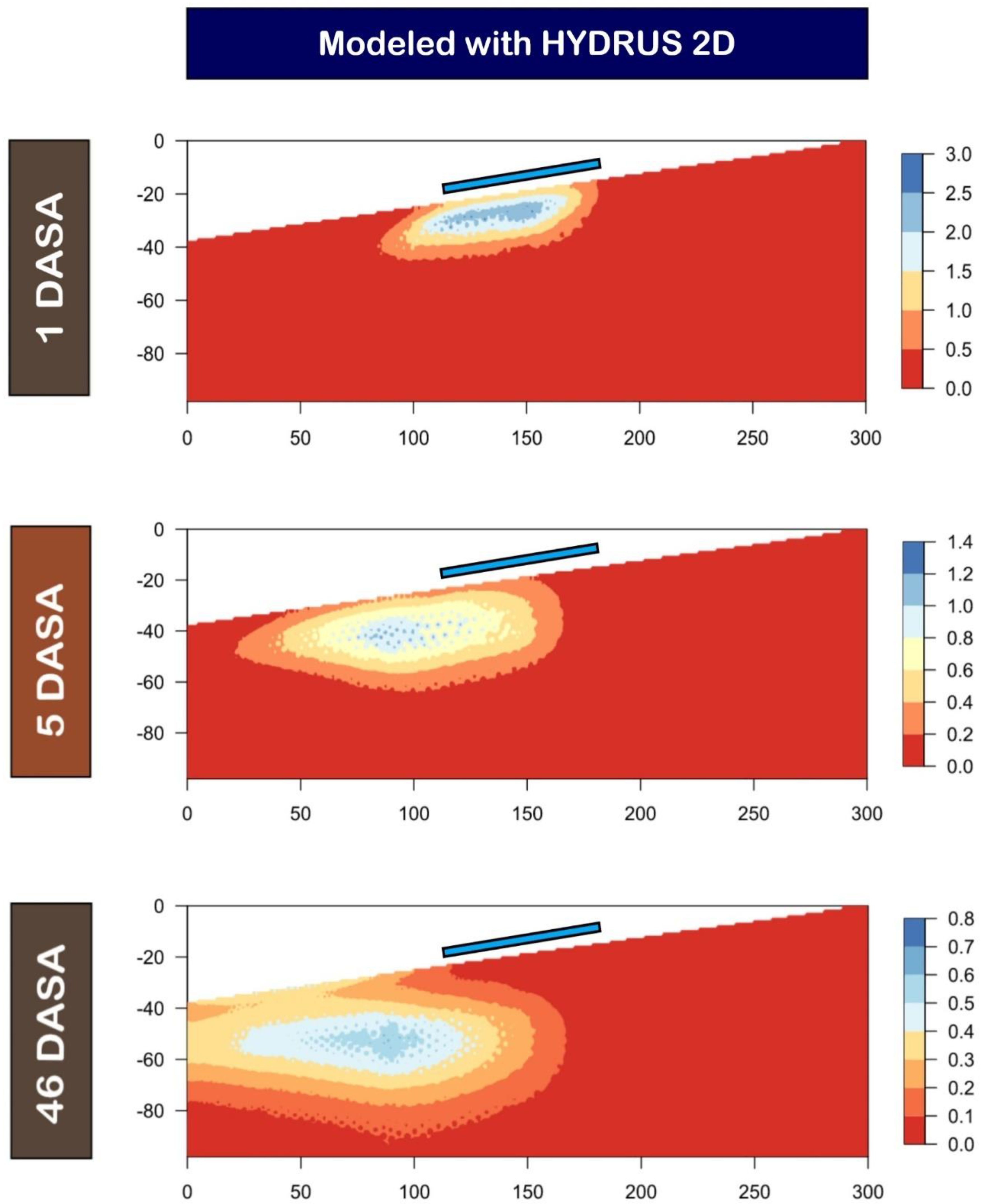
One of the main advantages of modelling with HYDRUS 2D is its versatility to simulate and graphically represent the solute movement within the soil domain under specific boundary conditions with a time progression. Using this approach, it was predicted that Br− moved as a plume preferentially along the slope, following the horizon boundary (Figure 5). This result agrees with our field findings for both sampling dates, where the subsurface lateral movement was more evident within the Ap horizon (Figure 4).
One day after the solute application (1 DASA), the highest concentration in the field plot was mostly located in the first 10 cm right below the application area (Figure 5). Over time, the plume moved both vertically and laterally, but the movement was more pronounced laterally mainly due to limited infiltration into the Bt horizon with lower hydraulic conductivity. For instance, the model predicted that Br− moves parallel to the soil surface and slightly towards deeper layers within the soil matrix during the first sampling date (5 DASA).
Interestingly, the model predicted a resurfacing of Br− traces when the plume was 110 cm away from the application center, with an increase in Br− concentration at shallower depths reaching values from 0.4 and 0.5 mg cm−3 during the second sampling date (46 DASA) (Figure 5). This was probably due to imposing evaporation and lack of water infiltration during the corresponding period (Figure 2).
The model tended to overestimate solute concentration specifically in the farthest point downslope of the experimental plot (Figure 5), where calculated values were almost twice as high as those obtained from measured data, but the model correctly predicted the directionality of the movement.
4. Discussion
4.1. Lateral Solute Transport
Filipović et al. [13] observed relatively little lateral subsurface movement of the tracer under rainstorm events in a layered soil when the phenomenon was studied through simulations with HYDRUS 2D. Even though their results are based on simulations from a “virtual experiment”, they highlighted the importance of several factors involved in the subsurface lateral flow, such as abrupt changes in the physical and hydrological properties of soil between neighboring horizons or underlying horizons, the timing and location of the tracer application, and the presence of extreme rainfall events.
Under sloped conditions, the lateral transport of solutes through soil may represent an important process in solute fate, with the magnitude depending on the water input amount (i.e., rainfall or irrigation), and the antecedent soil water content [11,12]. In addition, the differing magnitude of hydraulic properties due to variations in soil horizons with contrasting texture becomes a crucial factor for subsurface lateral flow [7,8,13,14]. Our experimental area presented those conditions (Table 1), and subsurface lateral flow was confirmed on the basis of both observed and simulated Br− movement documented (Figure 4 and Figure 5). The clear formation of a plume moving along the slope and the Ap horizon provided evidence that subsurface lateral flow might be a significant but underestimated water and solute movement mechanism. Moreover, the results indicated that special attention must be paid to reductions in hydraulic conductivity in lower soil profiles when determining the risk of subsurface lateral movement.
Having subsurface lateral movement at rates that are higher than the vertical flow can result in the underestimation of nonpoint source pollution by risk models that base their analysis on runoff and infiltration rates. Importantly, as shown in our model (Figure 5), subsurface lateral movement can maintain solutes closer to the soil surface, making the accumulation of high concentrations possible that could impact plant growth, as suspected by turfgrass managers in the case of herbicide injury downslope or generate a second phase of runoff risk. [5,6,36]
4.2. Caveats
Because Br− was used as an indicator for solute movement instead of herbicides and fertilizers, the results could be potentially considered a “worst case scenario”. The rate of solute movement with Br− is considerably higher than that for elements and organic molecules that have the capacity to adsorb to soil particles. Nevertheless, the movement in soil with herbicides and fertilizers is also water mediated, so although the rate might be different, the directionality of their movement should be similar to that of Br−. Unlike previous studies based solely on modeled data [13], the fact that the research reported here used field observations (Figure 4) provides more reliable evidence for the directionality of subsurface lateral solute movement.
The present study was conducted on a relatively small area (Figure 1), which had a slope that can be considered moderate in many turfgrass systems. If this factor influenced the outcome of the results, it likely did so by underestimating the magnitude of the subsurface lateral flow and solute transport. Longer and steeper slopes would favor faster movement and higher accumulation of solutes at the bottom of the slope.
4.3. Practical Implications
Nonpoint source pollution due to the movement of chemicals, including pesticides, has been a subject of great interest for developing best management practices in turfgrass, especially because turfgrass systems represent a large portion of urban and highly populated rural landscapes [37,38]. While runoff is considered the most important mechanism for pesticide transport to surface water bodies, next to wind-caused drift during application, their subsurface transport can also be significant in soils with coarse-textured surface horizon over fine-textured subsoil [39,40,41]. This is likely the result of the fact that runoff is easier to quantify than subsurface lateral movement, and that its effects on aboveground plant integrity are more visible, especially when herbicides or fertilizers are involved [5]. The present study showed the importance of their lateral movement at the subsurface level when considering the risk of nonpoint source pollution (Figure 4). The fact that percolated pesticides can resurface downslope (Figure 5), depending on the level of vertical variations in soil hydraulic properties, highlights the importance of pathways other than surface runoff that can determine the fate of the applied pesticides and their impact on ecosystems.
Our findings are particularly relevant to consider the implications of off-target movement of agricultural inputs such as herbicides, pesticides, and fertilizers in turfgrass landscapes, where ponds and creeks as well as ornamental plants and turf species could be negatively affected. Modeling approaches, as the one used here, can be a particularly valuable tool for assessing the likelihood of subsurface lateral movement in turfgrass systems with irregular topography common in golf courses, lawns, and recreational areas [42,43]. This predictive approach could be coupled with geographical information systems (GIS) to identify areas with high risk of herbicide and pesticide off-target movement and accumulation, allowing the optimization of their application [44]. Furthermore, this system does not have to be limited to reactive or remedial actions, but instead, it can be used in a preventive manner. For example, turfgrass and landscaping involve design and construction practices that may significantly alter topography and soil profile through the application of artificially made soil (e.g., mixing sand, mulch, and other materials with parent material), creating variability in slope and abrupt changes in soil layers with contrasting properties. Thus, our findings can inform the design and construction of landscapes to prevent subsurface lateral water movement. Furthermore, identifying the areas with a higher risk of subsurface lateral movement allows the use of management practices that mitigate that risk and prevent negative impacts on the turfgrass and the environment. For example, proper selection of herbicides and fertilizers with chemical properties that diminish the movement (such as herbicides with high sorption to soil particles, slow-release fertilizer formulations, and low-intensity irrigation) can be selected for turf management practices. If the areas of high risk are clearly defined, the use of low herbicide and fertilizer rates are another alternative to reduce the risk of off-target movement.
5. Conclusions
The first objective of the present study investigated the potential subsurface lateral movement of solutes in a sloped soil with divergent surface and subsurface soil textures. The results confirmed that water and solutes can move laterally faster than vertically within the soil profile, forming a plume that moves along the slope and the soil textural transition layer. To meet the second objective of the project, field data were used to develop a model that provided a mechanistic view of how subsurface lateral flow operates in a sloped turfgrass system. This model gave an explanation to the observations of turfgrass managers that herbicide injury can occur downslope from where herbicides are applied without exhibiting the injury pattern usually associated with runoff. [6] The experimental approach used here was designed to prevent surface runoff. This allowed us to reliably attribute to subsurface movement the detection of the tracer downslope from the application area. A challenge for future research will be to develop ways to quantitively differentiate the magnitude of surface and subsurface lateral movement under field conditions, especially during and after intense rainfall events. This will be critical for improving nonpoint pollution risk models.
The results described here have implications not only for turfgrass but for other agricultural and horticultural systems, where pesticides and fertilizers are applied to the soil, and topographic, edaphic, and climatological conditions can favor off target movement, negatively impacting the integrity of the crop and other organisms.
Author Contributions
Conceptualization, M.E.C., T.W.G., A.A., J.L.H. and R.G.L.; methodology, M.E.C., C.A.F.-U., A.A., and R.G.L.; formal analysis, M.E.C., J.L.H. and C.A.F.-U.; investigation, M.E.C.; resources, T.W.G., J.L.H. and R.G.L.; data curation, M.E.C.; writing—original draft preparation, M.E.C., C.A.F.-U. and R.G.L.; writing—review and editing, A.A., J.L.H. and R.G.L.; supervision, R.G.L.; project administration, R.G.L.; funding acquisition, T.W.G. and R.G.L. All authors have read and agreed to the published version of the manuscript.
Funding
This research was funded by a grant from the Center for Turfgrass Environmental Research and Education (CENTERE), as well as USDA-Hatch (NC-02653) and North Carolina Agriculture Research Service (NCARS). Manuel Camacho received partial financial support from the University of Costa Rica (OAICE-684-2021).
Data Availability Statement
Data will be provided upon request.
Acknowledgments
We would like to thank Adam Howard, Raymond McCauley, Marty Parish, and Daniel Freund for technical advice and support. The use of trade names in this publication does not imply endorsement of the products named or criticism of similar ones not mentioned by CENTERE, USDA, and NCAR.
Conflicts of Interest
The authors declare that they have no known competing financial interest or personal relationship that could have appeared to influence the work reported in this paper.
References
- Oerke, E.C. Crop losses to pests. J. Agric. Sci. 2006, 14, 31–43. [Google Scholar] [CrossRef]
- Haith, D.A.; Rossi, F.S. Risk assessment of pesticide runoff from turf. J. Environ. Qual. 2003, 32, 447–455. [Google Scholar] [CrossRef]
- Lee, S.J.; Mehler, L.; Beckman, J.; Diebolt-Brown, B.; Prado, J.; Lackovic, M.; Calvert, G.M. Acute pesticide illnesses associated with off-target pesticide drift from agricultural applications: 11 States, 1998–2006. Environ. Health Perspect. 2011, 119, 1162–1169. [Google Scholar] [CrossRef] [PubMed] [Green Version]
- Cessna, A.J.; McConkey, B.G.; Elliott, J.A. Herbicide transport in surface runoff from conventional and zero—Tillage fields. J. Environ. Qual. 2013, 42, 782–793. [Google Scholar] [CrossRef] [Green Version]
- Leon, R.G.; Unruh, J.B.; Brecke, B.J. Relative lateral movement in surface soil of amicarbazone and indaziflam compared with other preemergence herbicides for turfgrass. Weed Technol. 2016, 30, 229–237. [Google Scholar] [CrossRef]
- Gannon, T.W.; (North Carolina State University, Raleigh, NC, USA); Leon, R.G.; (North Carolina State University, Raleigh, NC, USA). Personal communication, 2018.
- Hardie, M.A.; Doyle, R.B.; Cotching, W.E.; Lisson, S. Subsurface lateral flow in texture-contrast (duplex) soils and catchments with shallow bedrock. Appl. Environ. Soil Sci. 2012, 2012, 861358. [Google Scholar] [CrossRef] [Green Version]
- Zaslavsky, D.; Sinai, G. Surface Hydrology: III Causes of lateral flow. J. Hydraul. Div. 1981, 107, 37–52. [Google Scholar] [CrossRef]
- Dusek, J.; Vogel, T. Modeling subsurface hillslope runoff dominated by preferential flow: One-vs. two-dimensional approximation. Vadose Zone J. 2014, 13, 1–13. [Google Scholar] [CrossRef]
- Dusek, J.; Vogel, T.; Sanda, M. Hillslope hydrograph analysis using synthetic and natural oxygen-18 signatures. J. Hydrol. 2012, 475, 415–427. [Google Scholar] [CrossRef]
- Kahl, G.; Ingwersen, J.; Nutniyom, P.; Totrakool, S.; Pansombat, K.; Thavornyutikarn, P.; Streck, T. Micro-Trench experiments on interflow and lateral pesticide transport in a sloped soil in Northern Thailand. J. Environ. Qual. 2007, 36, 1205–1216. [Google Scholar] [CrossRef]
- Kim, H.J.; Sidle, R.C.; Moore, R.D. Shallow lateral flow from a forested hillslope: Influence of antecedent wetness. Catena 2005, 60, 293–306. [Google Scholar] [CrossRef]
- Filipović, V.; Gerke, H.H.; Filipović, L.; Sommer, M. Quantifying subsurface lateral flow along sloping horizon boundaries in soil profiles of a hummocky ground moraine. Vadose Zone J. 2018, 17, 1–12. [Google Scholar] [CrossRef] [Green Version]
- McCord, J.T.; Stephens, D.B.; Wilson, J.L. Hysteresis and state dependent anisotropy in modeling unsaturated hillslope hydrologic processes. Water Resour. Res. 1991, 27, 1501–1518. [Google Scholar] [CrossRef]
- Milesi, C.; Running, S.W.; Elvidge, C.D.; Dietz, J.B.; Tuttle, B.T.; Nemani, R.R. Mapping and modeling the biogeochemical cycling of turf grasses in the United States. Environ. Manag. 2005, 36, 426–438. [Google Scholar] [CrossRef]
- Petrovic, A.M.; Easton, Z.M. The role of turfgrass management in the water quality of urban environments. Int. Turfgrass Soc. Res. J. 2005, 10, 55–69. [Google Scholar]
- Smith, A.E.; Bridges, D.C. Movement of certain herbicides following application to simulated golf course greens and fairways. Crop Sci. 1996, 36, 1439–1445. [Google Scholar] [CrossRef]
- Blake, G.R.; Hartge, K.H. Bulk density. In Methods of Soil Analysis, Part 1, Physical and Mineralogical Methods; Klute, A., Ed.; American Society of Agronomy: Madison, WI, USA, 1986; pp. 363–375. [Google Scholar]
- Gee, G.W.; Orr, D. 2.4 Particle-size analysis. In Methods of Soil Analysis, Part 4—Physical Methods; Dame, J.H., Topp, G.C., Eds.; Soil Science Society of America: Madison, WI, USA, 2002; pp. 255–293. [Google Scholar]
- Klute, A.; Dirksen, C. Hydraulic Conductivity and Diffusivity: Laboratory Methods. In Methods of Soil Analysis, Part 1, Physical and Mineralogical Methods; Klute, A., Ed.; American Society of Agronomy: Madison, WI, USA, 1986; pp. 674–687. [Google Scholar]
- Dane, J.H.; Hopmans, J.W. 3.3.2 Laboratory. In Methods of Soil Analysis, Part 4—Physical Methods; Dame, J.H., Topp, G.C., Eds.; Soil Science Society of America: Madison, WI, USA, 2002; pp. 675–720. [Google Scholar]
- Grossman, R.B.; Reinsch, T.G. 2.1 Bulk density and linear extensibility. In Methods of Soil Analysis, Part 4—Physical Methods; Dame, J.H., Topp, G.C., Eds.; Soil Science Society of America: Madison, WI, USA, 2002; pp. 201–228. [Google Scholar]
- Topp, G.C.; Ferré, P.A. 3.1 Water Content. In Methods of Soil Analysis, Part 4—Physical Methods; Dame, J.H., Topp, G.C., Eds.; Soil Science Society of America: Madison, WI, USA, 2002; pp. 417–545. [Google Scholar]
- Klute, A. Water Retention: Laboratory Methods. In Methods of Soil Analysis, Part 1, Physical and Mineralogical Methods; Klute, A., Ed.; American Society of Agronomy: Madison, WI, USA, 1986; pp. 635–662. [Google Scholar]
- Abdalla, N.A.; Lear, B. Determination of inorganic bromide in soils and plant tissues with a bromide selective-ion electrode. Commun. Soil Sci. Plant Anal. 1975, 6, 489–494. [Google Scholar] [CrossRef]
- Šimůnek, J.; van Genuchten, M.T.; Šejna, M. Recent developments and applications of the HYDRUS computer software packages. Vadose Zone J. 2016, 15, 1–25. [Google Scholar] [CrossRef] [Green Version]
- Šimůnek, J.; Sejna, M.; van Genuchten, M.T. New features of version 3 of the HYDRUS (2D/3D) computer software package. J. Hydrol. Hydromech. 2018, 66, 133–142. [Google Scholar] [CrossRef] [Green Version]
- Boivin, A.; Šimůnek, J.; Schiavon, M.; van Genuchten, M.T. Comparison of pesticide transport processes in three tile-drained field soils using HYDRUS-2D. Vadose Zone J. 2006, 5, 838–849. [Google Scholar] [CrossRef] [Green Version]
- van Genuchten, M.T. A closed-form equation for predicting the hydraulic conductivity of unsaturated soils. Soil Sci. Soc. Am. J. 1980, 44, 892–898. [Google Scholar] [CrossRef] [Green Version]
- Leij, F.J.; van Genuchten, M.T.; Yates, S.R.; Russell, W.B. RETC: A computer program for analyzing soil water retention and hydraulic conductivity data. In Proc. Int. Workshop, Indirect Methods for Estimating the Hydraulic Properties of Unsaturated Soils; van Genuchten, M.T., Leij, F.J., Lund, L.J., Eds.; University of California: Riverside, CA, USA, 1991; pp. 263–272. [Google Scholar]
- Vogel, T.; van Genuchten, M.T.; Cislerová, M. Effect of the shape of the soil hydraulic functions near saturation on variably-saturated flow predictions. Adv. Water Resour. 2001, 24, 133–144. [Google Scholar] [CrossRef]
- Abit, S.M.; Amoozegar, A.; Vepraskas, M.J.; Niewoehner, C.P. Fate of nitrate in the capillary fringe and shallow groundwater in a drained sandy soil. Geoderma 2008, 146, 209–215. [Google Scholar] [CrossRef]
- Shinde, D.; Savabi, M.R.; Nkedi-Kizza, P.; Vazquez, A. Modeling transport of atrazine through calcareous soils from south Florida. Trans. ASABE 2001, 44, 251. [Google Scholar] [CrossRef]
- Radcliffe, D.E.; Šimůnek, J. Soil Physics with HYDRUS: Modeling and Applications; CRC Press: Boca Raton, FL, USA, 2010; 373p. [Google Scholar]
- R Studio Team. R Studio: Integrated Development for R. R Studio, Inc., Boston. 2015. Available online: http://www.rstudio.com/ (accessed on 30 July 2021).
- Guo, L.; Fan, B.; Zhang, J.; Lin, H. Occurrence of subsurface lateral flow in the Shale Hills Catchment indicated by a soil water mass balance method. Eur. J. Soil Sci. 2018, 69, 771–786. [Google Scholar] [CrossRef]
- Dietz, M.E.; Clausen, J.C.; Filchak, K.K. Education and changes in residential nonpoint source pollution. Environ. Manag. 2004, 34, 684–690. [Google Scholar] [CrossRef] [Green Version]
- Erickson, J.E.; Cisar, J.L.; Volin, J.C.; Snyder, G.H. Comparing nitrogen runoff and leaching between newly established St. Augustinegrass turf and an alternative residential landscape. Crop Sci. 2001, 41, 1889–1895. [Google Scholar] [CrossRef] [Green Version]
- Amoozegar, A.; Niewoehner, C.; Lindbo, D. Water flow from trenches through different soils. J. Hydrol. Eng. 2008, 13, 655–664. [Google Scholar] [CrossRef]
- Gali, R.K.; Cryer, S.A.; Poletika, N.N.; Dande, P.K. Modeling pesticide runoff from small watersheds through field-scale management practices: Minnesota watershed case study with chlorpyrifos. Air Soil Water Res. 2016, 9, 113–122. [Google Scholar] [CrossRef] [Green Version]
- Tiryaki, O.; Temur, C. The fate of pesticide in the environment. J. Biol. Environ. Sci. 2010, 4, 29–38. [Google Scholar]
- Dann, R.L.; Close, M.E.; Lee, R.; Pang, L. Impact of data quality and model complexity on prediction of pesticide leaching. J. Environ. Qual. 2006, 35, 628–640. [Google Scholar] [CrossRef] [PubMed]
- Urbina, C.A.F.; van Dam, J.; Tang, D.; Gooren, H.; Ritsema, C. Estimating macropore parameters for HYDRUS using a meta-model. Eur. J. Soil. Sci. 2021, 72, 2006–2019. [Google Scholar] [CrossRef]
- Anlauf, R.; Schaefer, J.; Kajitvichyanukul, P. Coupling HYDRUS-1D with ArcGIS to estimate pesticide accumulation and leaching risk on a regional basis. J. Environ. Manag. 2018, 217, 980–990. [Google Scholar] [CrossRef] [PubMed]
Figure 1.
Photograph of the experimental plot (A), and 3D schematic diagram of the soil profile (B) with dimensions, soil horizons depth, and soil moisture sensor locations within the plot.
Figure 1.
Photograph of the experimental plot (A), and 3D schematic diagram of the soil profile (B) with dimensions, soil horizons depth, and soil moisture sensor locations within the plot.

Figure 2.
Air temperature and atmospheric water balance assessed during the tracer experiment in Raleigh, NC, USA. Black arrows represent the soil sampling days. Gray and white background used to contrast consecutive months. Blue arrow represents the solute application date.
Figure 2.
Air temperature and atmospheric water balance assessed during the tracer experiment in Raleigh, NC, USA. Black arrows represent the soil sampling days. Gray and white background used to contrast consecutive months. Blue arrow represents the solute application date.

Figure 3.
Finite element grid in HYDRUS 2D representing the soil domain assessed to evaluate soil water content dynamics and solute lateral movement in soil mapped as Cecil series located in Raleigh, NC. Grid contains 8147 triangular elements and 4202 nodes. Red dots correspond to frequency domain reflectometry (FDR) sensors and dark red ovals correspond to the soil sampling points.

Figure 4.
Bromide distribution in the experimental plot assessed for three soil depths at two different sampling times in Raleigh, NC, USA. Bromide values (mg kg−1) were obtained from soil samples collected from the field. Numbers on the x- and y-axes represent the coordinates within the plot. White circle located in the center of the plot represents the solute application area. Red arrow shows the main slope direction.

Figure 5.
Simulations for Br− distribution and movement within soil domain in the model during three different dates. Simulations were conducted at 1, 5 and 46 days after solute application (DASA). Bromide values were simulated with HYDRUS 2D. The x- and y-axes in the soil domain are in cm. Light blue bar above the soil surface indicates the solute application area. Color scale bar units for Br− are in mg cm−3.


Table 1.
Selected soil physical properties for the soil (mapped as Cecil series) in the experimental plot in Raleigh, NC.
Table 1.
Selected soil physical properties for the soil (mapped as Cecil series) in the experimental plot in Raleigh, NC.
| Horizon | Depth (cm) | Ks (cm h−1) | Bulk Density * (g cm−3) | Porosity * (cm3 cm−3) | Sand (%) | Silt (%) | Clay (%) | A (cm−1) | n † | ϴs (cm3 cm−3) | ϴr (cm3 cm−3) |
|---|---|---|---|---|---|---|---|---|---|---|---|
| Ap | 0–18 | 36.32 ± 4.48 | 1.20 ± 0.04 | 0.55 ± 0.01 | 91 | 5 | 4 | 0.006 | 1.460 | 0.47 | 0.08 |
| Bt | 18–60 | 3.28 ± 1.25 | 1.32 ± 0.03 | 0.50 ± 0.01 | 21 | 11 | 68 | 0.015 | 1.085 | 0.46 | 0.27 |
* Average values ± standard error (n = 6). Ks: Saturated soil hydraulic conductivity. † Unitless.
Table 2.
Soil sampling depth intervals for Br− movement determination.
| Date | Sampling Depth Intervals (cm) |
|---|---|
| 5 days after solute application | 0–15 |
| 15–30 | |
| 30–40 | |
| 40–50 | |
| 46 days after solute application | 0–5 |
| 5–10 | |
| 10–15 | |
| 15–30 | |
| 30–45 |
Table 3.
Statistical parameters to assess overall model performance while predicting soil water content and bromide concentration with HYDRUS 2D.
Table 3.
Statistical parameters to assess overall model performance while predicting soil water content and bromide concentration with HYDRUS 2D.
| Predicting Variable | Statistical Parameter * | Modeled with HYDRUS 2D |
|---|---|---|
| Soil water content (cm3 cm−3) | RMSE (cm3 cm−3) | 0.030 |
| d | 0.941 | |
| NSE | 0.802 | |
| Bromide concentration (mg cm−3) | RMSE (mg cm−3) | 0.453 |
| d | 0.247 | |
| NSE | –0.030 |
* RMSE: Root mean square error; d: Willmott agreement index; NSE: Nash-Sutcliffe efficiency.
Disclaimer/Publisher’s Note: The statements, opinions and data contained in all publications are solely those of the individual author(s) and contributor(s) and not of MDPI and/or the editor(s). MDPI and/or the editor(s) disclaim responsibility for any injury to people or property resulting from any ideas, methods, instructions or products referred to in the content. |
© 2023 by the authors. Licensee MDPI, Basel, Switzerland. This article is an open access article distributed under the terms and conditions of the Creative Commons Attribution (CC BY) license (https://creativecommons.org/licenses/by/4.0/).
Share and Cite
MDPI and ACS Style
Camacho, M.E.; Faúndez-Urbina, C.A.; Amoozegar, A.; Gannon, T.W.; Heitman, J.L.; Leon, R.G. Subsurface Lateral Solute Transport in Turfgrass. Agronomy 2023, 13, 903. https://doi.org/10.3390/agronomy13030903
AMA Style
Camacho ME, Faúndez-Urbina CA, Amoozegar A, Gannon TW, Heitman JL, Leon RG. Subsurface Lateral Solute Transport in Turfgrass. Agronomy. 2023; 13(3):903. https://doi.org/10.3390/agronomy13030903
Chicago/Turabian StyleCamacho, Manuel E., Carlos A. Faúndez-Urbina, Aziz Amoozegar, Travis W. Gannon, Joshua L. Heitman, and Ramon G. Leon. 2023. "Subsurface Lateral Solute Transport in Turfgrass" Agronomy 13, no. 3: 903. https://doi.org/10.3390/agronomy13030903
Note that from the first issue of 2016, this journal uses article numbers instead of page numbers. See further details here.