Advanced Data Analysis as a Tool for Net Blotch Density Estimation in Spring Barley


1
Control Engineering, Environmental and Chemical Engineering Research Unit, University of Oulu, 90014 Oulu, Finland
2
Natural Resources Institute Finland, 31600 Jokioinen, Finland
*
Author to whom correspondence should be addressed.
Agriculture 2020, 10(5), 179; https://doi.org/10.3390/agriculture10050179
Submission received: 27 April 2020
/
Revised: 12 May 2020
/
Accepted: 14 May 2020
/
Published: 19 May 2020
(This article belongs to the Section Crop Protection, Diseases, Pests and Weeds)
Abstract
:A novel data analysis method for the evaluation of plant disease risk that utilizes weather information is presented in this paper. This research considers two different datasets: open weather data from the Finnish Meteorological Institute and long-term (1991–2017) plant disease severity observations in different hardiness zones in Finland. Historical net blotch severity data on spring barley were collected from official variety trials carried out by the Natural Resources Institute Finland (Luke) and the analysis was performed with existing data without additional measurements. Feature generation was used to combine different datasets and to enrich the information content of the data. The t-test was applied to validate features and select the most suitable one for the identification of datasets with high net blotch risk. Based on the analysis, the selected daily measured variables for the estimation of net blotch density were the average temperature, minimum temperature, and rainfall. The results strongly indicate that thorough data analysis and feature generation methods enable new tools for plant disease prediction. This is crucial when predicting the disease risk and optimizing the use of pesticides in modern agriculture. Here, the developed system resolves the correlation between weather measurements and net blotch observations in a novel way.
1. Introduction
Barley, Hordeum vulgare L., is a cereal plant of the grass family Poaceae. It is the fourth largest grain crop, and it was grown globally on 47 million hectares in 2016 [1]. Barley is primarily grown as animal fodder and as a source of malt for alcoholic beverages, but is also commonly used in food products, e.g., breads, soups and stews, and health products. However, barley production is challenged by several biotic and abiotic pressure factors. On average, plant diseases caused by microbes can decrease the annual average yield of the barley crop by up to 20% [2]. One of the most commonly distributed fungal diseases in barley is net blotch, which is caused by the ascomycete Pyrenophora teres Drechsler. In Finland, net blotch was present in 86% of barley fields investigated in 2009 [3]. The pathogen overwinters on barley debris or seed. During the growing season, it reproduces asexually on barley leaves. The symptoms start as small brown lesions, which elongate and produce dark brown streaks across the leaf blades, creating a net-like pattern surrounded by a yellow margin. Environmental conditions play a significant role in disease development. The leaf wetness period that is required for conidium germination relates to the temperature. In studies by van den Berg and Rossnagel [4], it was shown that the minimum leaf wetness period required for P. teres infection was halved as the temperature was doubled in degrees Celsius. Martin and Clough [5] reported that the spore release of P. teres correlated positively with temperature, but negatively with relative humidity and leaf wetness. In addition to the environmental factors, the host plant and agricultural factors influence the development of disease epidemics. Plants have evolved different resistance mechanisms against pathogens, and barley varieties vary in tolerance and resistance [6].
To avoid the negative impacts of agrochemicals, legal obligations have been established at global and national levels. The optimization of chemical control is one of the key issues in Integrated Pest Management (IPM), which in the European Union has been codified into the form of a directive. According to the IPM directive, chemical protection needs to be justified and well documented [7].
Accurate prediction, or disease forecasting, plays an important role when optimizing the use of agrochemicals. In Abdullah et al. [8], the excessive usage of pesticides in Pakistan is briefly discussed. The authors have shown that data mining integrated with agricultural data, e.g., pest scouting, pesticide usage and meteorological recordings, is a useful tool for pesticide optimization. Overall, data analysis and modeling as well as knowledge of plant diseases are the components of reliable disease forecasting [9]. The article by Kerr and Keane [10] discusses the prediction of disease outbreaks with details. The authors present the basis of plant disease prediction and deal with the information extensively with examples. According to the authors, disease forecasting is the use of both weather data and biological data to predict disease incidence [10]. Another way to predict diseases that was mentioned is based on the monitoring of the highs and lows of an annual disease cycle.
Sentelhas et al. [11] have studied the parameters influencing plant disease occurrence and pointed out the importance of leaf wetness duration (LWD) in plant disease warning systems. In the article, the LWD measuring system and the effects of sensor positioning are discussed. However, measurement of leaf wetness duration is problematic because of the lack of a standard sensor and the lack of a standard exposure protocol.
Kim et al. [12] reported that costly and arduous measurements could be replaced with a reliable estimation of LWD. The authors [12] presented an extensive literature survey of LWD estimation with a comparison of the reported LWD models. They applied some corrections to existing models (e.g. a height correction to SkyBit wind speed estimates) to enhance estimation accuracy. The model-derived estimates utilized hourly weather data from 15 weather stations in Iowa, Illinois, and Nebraska during May to September in 1997, 1998 and 1999 [12]. Furthermore, the modeling of LWD and estimation accuracy have been studied by Sentelhas et al. [13] and the usability of weather radar data in a plant disease management system has been studied by Rowlandson et al. [14].
Data analysis and machine learning have been utilized in agriculture and several applications have been published. Bhor et al. [15] presented a framework for an agricultural web portal, which helps farmers to predict crop diseases and prevent economic losses. Furthermore, various articles [16,17,18,19] have demonstrated the utilization of data analysis and modeling in crop farming and plant breeding. Big data technology in plant science has been reviewed in an article by Ma et al. [20]. A more general presentation of the principles of big data analysis and some applications are reviewed in the article by Tien [21]. One research study about plant diseases and crop production simulation as a tool for farmers’ decision-making is presented in an article by Bregaglio and Donatelli [22].
Wang et al. [23] have used the deep learning approach in the estimation of plant disease severity. The authors trained a neural network to classify apple black rot severity using the images from an open access database, PlantVillage, with promising results. Moreover, the deep learning technique has been utilized in an image-based, real-time approach to detect diseases and pests in tomato plants [24]. The effects of plant diseases, pests, weather conditions, and climate issues are topics with the highest priority in agriculture, and the reliable prediction of phenomena affecting the crop is a valuable tool in modern agriculture.
However, the complexity or unreliability of models and the difficulties in obtaining informative data or performing reliable observations may complicate the applicability of present plant disease forecasting methods. The main contribution of this paper is to show that by combining the information from existing measurements with data mining methods (feature generation and analysis), years with a high risk for net blotch can be distinguished from years with a smaller risk even in the early stage of the growing season using existing measurements. This information forms the basis for predicting net blotch occurrence that can be used in deciding on the use of pesticides. To avoid complex model structures, multiple models, and the costs of extra measurement arrangements, this research aims solely at combining existing data from different sources, public and private. The resulting methodology is available for future routine analysis without any specific tests. In addition to data analysis, the usability of open weather data is demonstrated and discussed.
2. Materials and Methods
This study combines information from two different datasets—weather measurements and the prevalence of net blotch at the observation fields. During the research, no extra measurements were arranged; instead, the available data were mathematically combined for a new purpose. The principle of this study is presented in Figure 1.
Net blotch data had been collected and pre-processed by the Natural Resources Institute Finland (Luke) during the years 1991–2017. The numerical data used in this research exists in the Oracle database. Measurements included information about the observation year, field location (municipality), cultivated barley genotype, and the disease severity of net blotch. The test fields were located in Central and Southern Finland. In this research, the net blotch observation data from hardiness zones I–IV were utilized. The approximate locations of the observation fields can be seen in Figure 2. The data analysis, feature generation, and evaluation steps were exactly the same in each of the four cases.
Field experiments had been conducted in 1991–2017 in different locations in Finland, representing areas where spring barley is typically grown. Experiments were included as part of the Official Variety Trials and they all followed the standard procedures specified for that purpose [25]. These were managed by Luke Finland at its numerous regional research units and by plant breeding companies and private agricultural research stations. All experiments were arranged as randomized complete block designs or incomplete block designs. The number of replicates varied from three to four depending on the location and year. In each year, the set of cultivars and breeding lines changed, but only partly; long-term check cultivars were also used. A typical trial included 30 cultivars. Long-term check cultivars ensure that, in any well-defined linear model analysis, the effects of cultivars and environments can always be estimated [26].
The plots were 7–10 m × 1.25 m, depending on the location and year. The seeding rate was 450–550 viable seeds per square metre, conforming to the commonly used seeding rates in Finland. Fertilizer use depended on cropping history, soil type, and fertility. Weeds and pests were chemically controlled with the active ingredients largely used in commercial farming. However, diseases were not controlled with fungicides.
The disease pressure, a risk index depending on environmental factors and the genotype of cereal, is quantified by Luke Finland by means of equation 1 and using the following steps. The effects of the environment and genotype were separated by the following statistical model based on the structure of the data collection:
where yijk is the observed value for the ith cultivar in the jth year and the kth experimental site. In addition, all experiments have 3 or 4 replications, and the replication is a nested factor: replication l is nested in the environmental effect of the jth year and kth experimental site. Parameter µ is the intercept, bl(jk) is the random effect of the lth replication, gi the effect of the ith genotype, ejk is the effect of the environment, geijk is the error term for the environmental effect, and εijkl is the residual. For the incomplete block design, the effect of the block was divided into two parts: variance between incomplete and complete blocks.
yijkl = µ + bl(jk) + gi + ejk + geijk + εijkl
In this research, the estimated values of the environment, , are mutually comparable estimates, i.e., despite the fact that the set of genotypes (cultivars) varied between trials and disease resistance between genotypes vary, trials can be put into order according to the disease pressure. This is important because modern genotypes have a higher disease resistance than older genotypes. The estimated values (per year and location) were scaled into three categories: 0 (maximum value 0.5%), 1 (0.6–5%), and 2 (over 5.1%). One example of the scale for appraising plant disease severity in cereals is presented in Saari and Prescott [27].
The weather data were obtained from the open database of the Finnish Meteorological Institute (FMI). More information about FMI open weather data is available in the report by Honkola et al. [28]. In every presented case, the distance between the local weather station and the observation field was the same throughout the observation years. The information content of weather data was compared during the whole period under the review. The loaded data were in the .xlsx format and usable in MATLAB®. The variables analyzed in this study were:
- place of observation,
- date of observation,
- rainfall per day [mm], R,
- average temperature per day, Tav [°C],
- daily minimum temperature, Tmin [°C], and
- daily maximum temperature, Tmax [°C].
The FMI data included some missing information and the data required further pre-processing. First, FMI data were arranged into datasets according to the year of observation. The datasets which included consecutive missing observations were discarded at this stage. The FMI datasets were then grouped according to the observation place and the net blotch category (0–2). Later, the datasets in the 0-category were referred to as the reference data and the datasets from categories 1 or 2 were compared to them. Four years’ data of independent weather observations from each hardiness zone and each net blotch category were utilized, except for hardiness zone IV and category 0 data, where measurements from three years were available. Brief information about the utilized data is presented in Table 1. It is important to notice that the different datasets were later indexed both spatially and temporally. The particular years and weather stations related to the data used are presented in Appendix A.
The net blotch observation data included one value per year while the weather data consisted of daily observations. The number of weather variables was four in each analysis and the number of tested feature candidates was 1760.
Because of the different weather conditions, the beginning of the growing season and the sowing date varied according to the year and the observation field. This must be taken into account in deciding the starting point of the analyzed period (to). Two variants were compared in this study. The first one defined the starting point as the beginning of the growing season, defined as the time when the mean temperature remained over plus five degrees Celsius for five consecutive days. In the second variant, the sowing date was used as the starting point. The data before this starting point and after the growing season was omitted. The analyzed period was 14 days from the starting point.
All of the data analysis and result evaluation were performed in the MATLAB® programming environment. First, the statistical values of the weather measurements were analyzed to find out whether the reference data differed from the datasets in category 1 or 2. The mean value of daily rainfall, R [mm], increased as well as the net blotch category when referring to the datasets related to the beginning of the growing season. In most cases with the datasets starting from the sowing date, R also increased by net blotch category, but in the case of hardiness zone III, categories 0 and 2 had the same mean R value. The statistical characteristics of the variables are presented in Table 2.
The feature generation was performed because it was not possible to classify the datasets into different net blotch categories with the initial calculated statistical values. This means that new computational variables were generated from the original data by mathematical operations and the features with the highest information content were selected by using the t-test. More information about the feature generation methods is published, for example, in [29,30,31,32,33].
The feature generation method used in this study is presented by Ruusunen [34] (p. 50). The method used composes new variables from the original ones (R, Tav, Tmax, and Tmin) with different mathematical operations, such as addition, subtraction, multiplication, division, involution, logarithm, square root, and combinations of them. A list of possible feature prototypes which were generated as mentioned above are presented with details in [34] (Appendix A). All of those candidates were tested in this study and the feature validation was performed with the t-test. The utilization of the t-test was carried out in a MATLAB® environment with the function t-test2 and 70% confidence intervals. Two-sample t-tests were selected with the assumption that the data vectors were from independent random samples with unknown variance. The selected features were then the candidates with which categories 1 or 2 could be separated with most certainty from the reference datasets (category 0). The data analysis procedure is presented in Figure 3.
The two-sample t-test was applied to evaluate the analysis results. In this case, where two data samples are assumed to be from populations with unequal variances, the test statistic t under the null hypothesis has an approximate Student’s t distribution with a number of degrees of freedom given by Satterthwaite’s approximation [35]. This arrangement can also be called Welch’s t-test.
3. Results and Discussion
The statistical characteristics (mean value, standard deviation, and median) of the weather data are listed in Table 2. The characteristics are indexed by variables, locations and net blotch categories, and analysis was performed for two alternatives of the starting point, to:t0 equals the beginning of the growing season and t0 equals the sowing time. From the statistical point of view, the weather conditions were quite similar in the selected years. The temperature increased from the beginning of the growing season to the sowing time, which is quite understandable since the beginning of the growing season was typically two to four weeks earlier than the sowing time.
All of the generated features were tested. The weather data belonging to net blotch categories 1 and 2 were compared with the reference data category 0 with the t-test and the following hypotheses:
H0.
the daily feature values have equal means and equal but unknown variances in tested datasets,
H1.
the daily feature values have unequal means.
The number of days and feature values from categories 1 and 2 that differed statistically from the reference data were computed. Feature generation and validation were demonstrated with the datasets (four years from category 0 and four years from category 2) from hardiness zone III and with the generated feature (Tmin2 x Tav2). The feature values from categories 0 and 2 are first presented in Figure 4, where the category 0 data points are marked by crosses (x) and category 2 data points as dots. The observation period is 14 days and t0, the starting point, is the beginning of the growing season.
In this case (Hardiness zone III), the null hypothesis was rejected nine times and accepted five times during the 14-day observation period. Then, the two tested datasets differed statistically with the feature generation technique and t-test with a 70% confidence interval in the case of nine days.
The results of analyzed locations and categories 0 compared to 1, and 0 compared to 2 are presented in Table 3.
As can be seen from Table 3, the separation ability of the most suitable features, where t0 equals the beginning of the growing season, was at least sufficient and in several cases statistically stronger than the separation ability of the datasets where t0 equals sowing dates. Consequently, the following results are presented only with the datasets where t0 equals the beginning of the growing season. It seems that the information content of the data varies during the growing season, and the optimal starting point for the analyzed time window has to be studied carefully.
Several features were generated from every spatial dataset with which the best separation results were achieved. The features that were the most suitable for separating the reference data and categories 1 and 2 are listed in Table 4. The original variables are marked as a, b, c, and d and are R, Tav, Tmax, and Tmin respectively. According to the t-test, the daily feature values included unequal means 8–11 times (out of 14) when comparing the reference data and category 1 data, and 9–11 times (out of 14) when comparing the reference data and category 2 data. The separation ability increased or remained the same when comparing categories 0 vs. 1 and 0 vs. 2, except for hardiness zone III.
The cumulative summed feature values (features of Table 4 for each hardiness zone) calculated for hardiness zones I–IV and categories 0 vs. 1 are presented in Figure 5 and those for categories 0 vs. 2 in Figure 6. The idea to test the cumulative sum here was based on the assumption that the growth of net blotch is some kind of dynamic phenomenon. Thus, the effects, for example, of rainfall were assumed to accumulate during the growing period. With the cumulative sum applied to the time series of listed features, the effectiveness of the utilization of these features can be demonstrated visually.
The separation ability of the presented features is shown in Figure 5 and Figure 6. The results show that the infected years can be potentially separated from the reference data using the weather measurements and the feature generation technique. Feature selection was based on summing up the number of days in a certain time window when the two datasets differed statistically at the 70% confidence level. Thus, for example, in Table 3 and in hardiness zone I, the day sums of 9 and 11 both indicate full classification capability with the method at the respective time. This way, the numbers in Table 3 are related to the robustness of the features against uncertainties in the measured data.
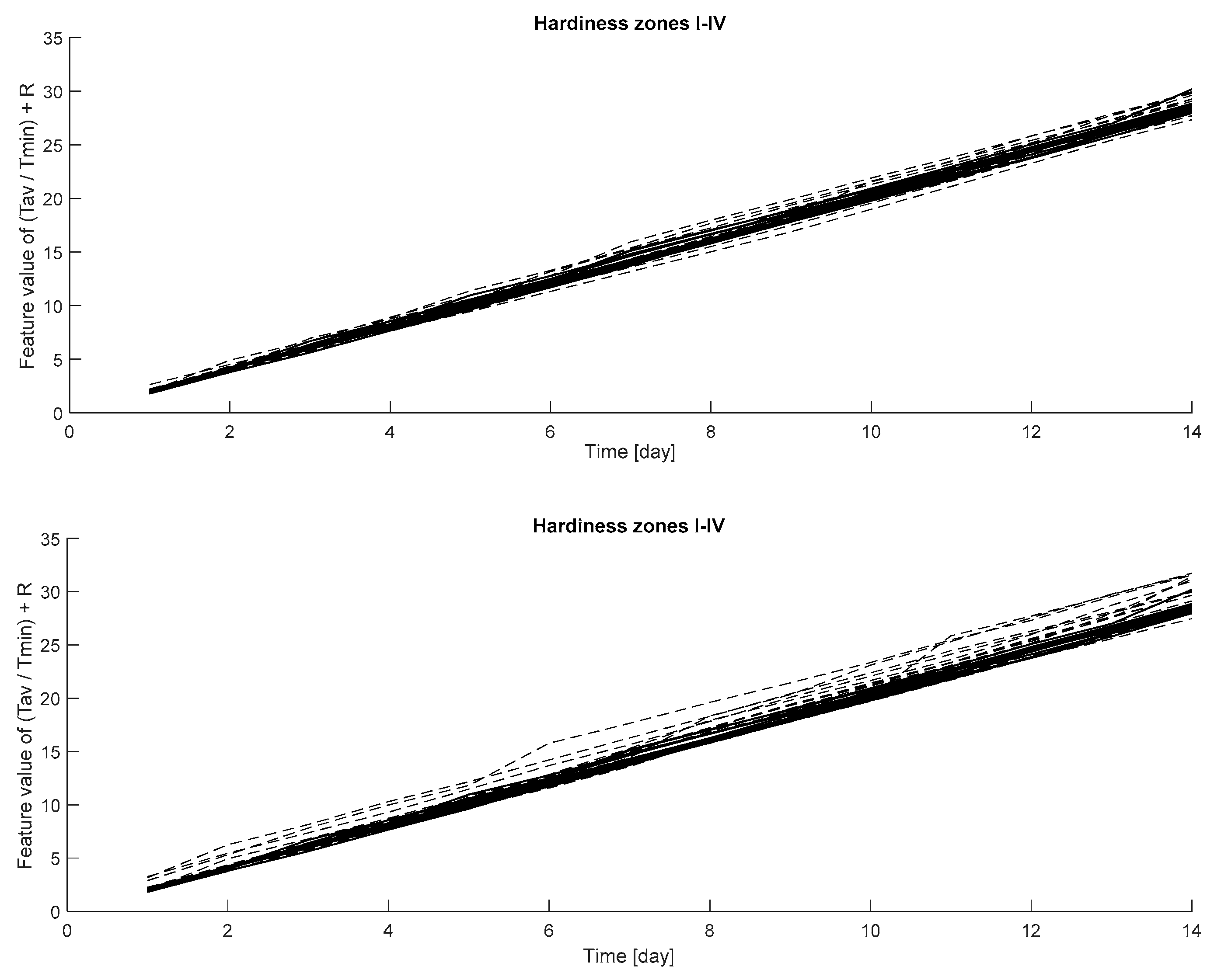
However, the best suitable features (selected by the t-test) depend on the hardiness zone and the estimation should be further extended to a form that is more general in order to increase practical usability of the analysis. For that reason, the hardiness zone I–IV datasets were merged and the earlier described analyzing steps were then performed. This new dataset included the weather measurements from 15 reference years, 16 category 1 years, and 16 category 2 years. The cumulative summed feature values for both cases are presented in Figure 7. The selected feature based on the analysis in the cases of the reference data vs. category 1 data and the reference data vs. category 2 data is Tav/Tmin + R.
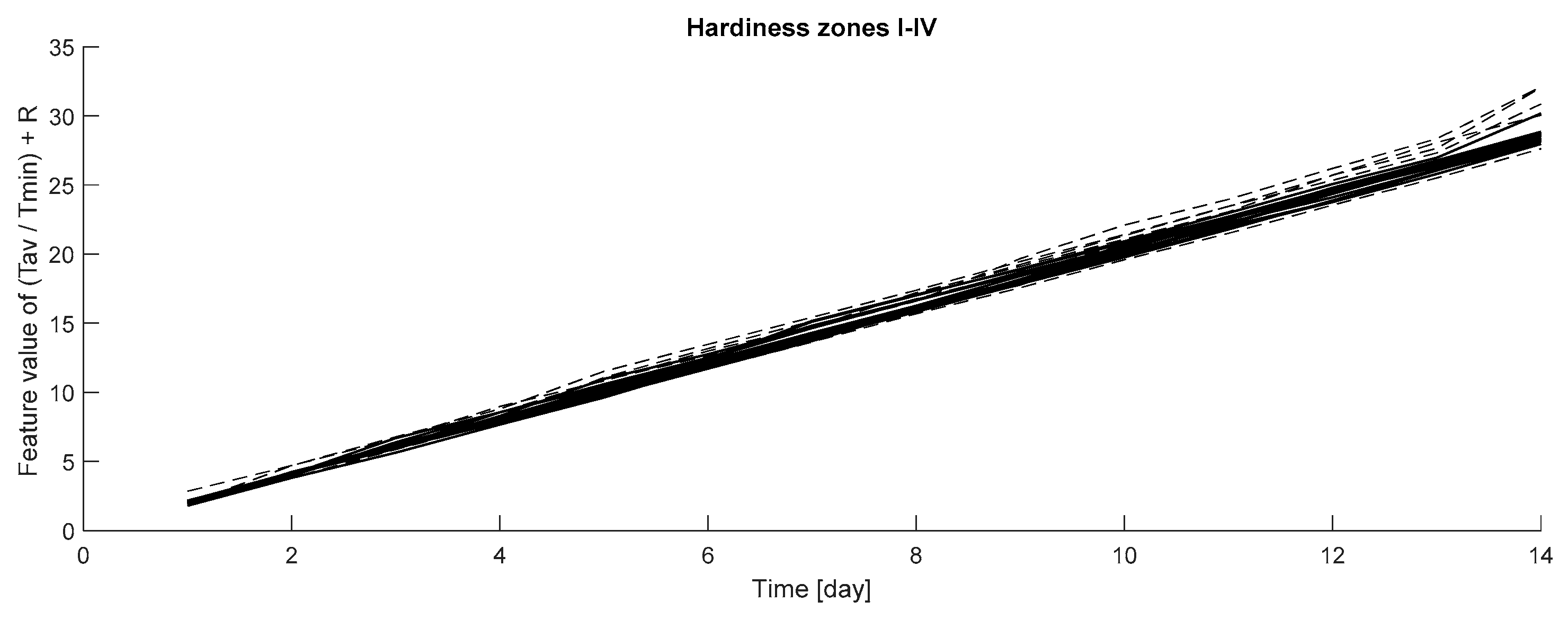
The classification task was repeated with the new independent dataset applying the same feature as above. Seven years’ data (category 2) was analyzed as described and compared to the original reference data (category 0). The classification results with the new dataset are presented in Figure 8.
The results are interesting and especially the lower graphs in Figure 7 and the graphs in Figure 8 show that there is a difference between the cumulative summed feature values when comparing the reference data and the category 2 data. Nevertheless, the classification accuracy needs to be improved, and therefore the generalization potentiality of the method needs further study.
4. Conclusions
Thorough statistical analyses of weather measurements and net blotch observations were performed, and the results are presented in this article. This research confirms that weather conditions have a significant effect on net blotch density. Using advanced data analysis, the information content of the existing weather measurements was enriched, and extra measurement campaigns were unnecessary. The feature generation and validation results show that the most suitable features were combinations of the original measurements, which supports the assumption that the influence of the weather and the infection of plants are a complex phenomenon.
The analysis was performed with data from four different hardiness zones, each zone separately, and also jointly as one set of data to test the generalization ability of the developed method. Each spatial dataset was also analyzed from the temporal point of view in a time window of 14 days using two datasets: one where the starting point, t0, is the very early stage of the growing season and the other where t0 is the sowing date. According to the analysis, the separation ability of datasets where t0 equals the beginning of the growing season was at least sufficient and, in several cases, statistically stronger than the separation ability of datasets where t0 equals sowing dates. However, the information content of the data varies during the growing season and the optimal date of t0 still needs thorough research.
The datasets were categorized according to the yearly net blotch density. Category 0 (no net blotch) was used as the reference data and the datasets from categories 1 and 2 were compared with that. The aim was to develop a method that can identify the increasing risk for barley net blotch and verify it with existing data. This method is valuable when predicting net blotch occurrence and possible need for pesticide use. The best suitable features were evaluated by the t-test. Here, the t-test was a sufficient evaluation method; however, the feature evaluation step still needs more research.
The reliable identification of the weather conditions that led to a net blotch infection can be utilized for modeling and eventually for the optimization of pesticides. The FMI open database includes reliable and usable weather measurements, and the applicability of public data has been demonstrated in this paper.
This study proves the effectiveness of data analysis and offers a new perspective for net blotch estimation. Accurate plant disease prediction is a valuable tool for optimizing pesticides and minimizing their harmful effects on the environment. To achieve a reliable model for net blotch forecasting, data on the combined four hardiness zones needs more research. The estimation accuracy and the generalization of the presented method need to be tested with new datasets. In addition, new measurements such as air humidity should be considered. In conclusion, justified and optimized chemical protection saves money and the environment in the long run and is part of sustainable agriculture.
Author Contributions
Conceptualization, O.R.; Formal analysis, O.R. and L.J.; Methodology, O.R. and M.R.; Supervision, K.L.; Writing—original draft, O.R., M.J. and L.J.; Writing—review & editing, M.J., L.J., M.R. and K.L. All authors have read and agreed to the published version of the manuscript.
Funding
This research was funded by the Ministry of Agriculture and Forestry of Finland, Document number 632/03.01.02/2017.
Conflicts of Interest
The authors declare no conflict of interest.
Appendix A: The Data Used
The weather data used has been downloaded from the FMI open database: https://www.ilmatieteenlaitos.fi/havaintojen-lataus#!/
Hardiness zone I: until year 2011, the FMI weather station “Turku airport” and 2012–2017 the FMI weather station “Kaarina, Yltöinen”.
Hardiness zone II: the FMI weather station “Jokioinen”.
Hardiness zone III: the FMI weather station “Seinäjoki, Pelmaa”.
Hardiness zone IV: the FMI weather station “Siikajoki, Revonlahti”.
| Weather Data, listed by Hardiness Zones and Net Blotch Density | |||
| Hardiness zone I, net blotch density <0.5% | Hardiness zone II, net blotch density <0.5% | Hardiness zone III, net blotch density <0.5% | Hardiness zone IV, net blotch density <0.5% |
| 1994 | 1993 | 1994 | 1992 |
| 1999 | 1994 | 2000 | 1993 |
| 2000 | 1999 | 2005 | 1994 |
| 2004 | 2006 | 2007 | |
| Hardiness zone I, net blotch density 0.6–5.0% | Hardiness zone II, net blotch density 0.6–5.0% | Hardiness zone III, net blotch density 0.6–5.0% | Hardiness zone IV, net blotch density 0.6–5.0% |
| 2002 | 2003 | 2004 | 1991 |
| 2005 | 2004 | 2006 | 2007 |
| 2007 | 2005 | 2011 | 2009 |
| 2011 | 2013 | 2013 | 2010 |
| Hardiness zone I, net blotch density >5.1% | Hardiness zone II, net blotch density >5.1% | Hardiness zone III, net blotch density >5.1% | Hardiness zone IV, net blotch density >5.1% |
| 2009 | 2014 | 2002 | 2012 |
| 2013 | 2015 | 2003 | 2013 |
| 2014 | 2016 | 2008 | 2014 |
| 2016 | 2017 | 2016 | 2015 |
| Validation | |||
| Hardiness zone I, net blotch density >5.1% | Hardiness zone II, net blotch density >5.1% | Hardiness zone III, net blotch density >5.1% | Hardiness zone IV, net blotch density >5.1% |
| 1998 | 1996 | 2009 | 1999 |
| 2008 | 1998 | 2000 | |
References
- FAO. FAOSTAT. 2016. Available online: http://www.fao.org/faostat/en/ (accessed on 13 July 2019).
- Murray, G.M.; Brennan, J.P. Estimating disease losses to the Australian barley industry. Australas. Plant Pathol. 2010, 39, 85–96. [Google Scholar] [CrossRef]
- Jalli, M.; Laitinen, P.; Latvala, S. The emergence of cereal fungal diseases and the incidence of leaf spot diseases in Finland. Agric. Food Sci. 2011, 20, 62–73. [Google Scholar] [CrossRef]
- Berg, C.G.J.; van den Rossnagel, B.G. Effects of temperature and leaf wetness period on conidium germination and infection of barley by Pyrenophora teres. Can. J. Plant Pathol. 1990, 12, 263–266. [Google Scholar] [CrossRef]
- Martin, A.R.; Clough, K.S. Relationship of airborne load of Pyrenophora teres and weather variables to net blotch development on barley. Can. J. Plant Pathol. 1984, 6, 105–110. [Google Scholar] [CrossRef]
- Jalli, M. The Virulence of Finnish Pyrenophora Teres f. Teres Isolates and Its Implications for Resistance Breeding. MTT Science 9. Ph.D. Thesis, Helsinki University, Helsinki, Finland, 2010. [Google Scholar]
- European Union. Directive 2009/128/EC of the European Parliament and the Council of 21 October 2009: Establishing a Framework for Community Action to Achieve the Sustainable use of Pesticides; Official Journal of the European Union L: Brussels, Belgium, 2009; Volume 309, pp. 71–86. [Google Scholar]
- Abdullah, A.; Brobst, S.; Pervaiz, I.; Umer, M.; Nisar, A.; Learning dynamics of pesticide abuse through data mining. In: Proceedings of the Second Workshop on Australasian Information Security, Data Mining and Web Intelligence, and Software Internationalization. ACSW Front. 2004, 32, 151–156. [Google Scholar]
- Hardwick, N.V. Disease Forecasting. The Epidemiology of Plant Diseases, 2nd ed.; Springer: Dordrecht, The Netherlands, 2006; pp. 239–267. [Google Scholar]
- Kerr, A.; Keane, P. Prediction of disease outbreaks. In Plant Pathogens and Plant Diseases; Brown, J.F., Ogle, H.J., Eds.; Rockvale Publications: Armidale, Australia, 1997; pp. 299–313. [Google Scholar]
- Sentelhas, P.C.; Gillespie, T.J.; Gleason, M.L.; Monteiro, J.E.B.A.; Helland, S.T. Operational exposure of leaf wetness sensors. Agric. For. Meteorol. 2004, 126, 59–72. [Google Scholar] [CrossRef]
- Kim, K.S.; Taylor, S.E.; Gleason, M.L.; Koehler, K.J. Model to enhance site-specific estimation of leaf wetness duration. Plant Dis. 2002, 86, 179–185. [Google Scholar] [CrossRef] [Green Version]
- Sentelhas, P.C.; Gillespie, T.J.; Gleason, M.L.; Monteiro, J.E.B.M.; Pezzopane, J.R.M.; Pedro, M.J., Jr. Evaluation of a Penman–Monteith approach to provide ‘‘reference’’ and crop canopy leaf wetness duration estimates. Agric. For. Meteorol. 2006, 141, 105–117. [Google Scholar] [CrossRef]
- Rowlandson, T.L.; Gillespie, T.J.; Ford, R.P. Application of Canadian weather radar data to plant disease management schemes in southern Ontario. Atmos. Ocean 2009, 47, 154–159. [Google Scholar] [CrossRef]
- Bhor, S.; Kotian, S.; Shetty, A.; Sawant, P. Developing An Agricultural Web Portal For Crop Disease Prediction Using Data Mining Techniques. Int. J. Recent Sci. Res. 2017, 8, 15507–15509. [Google Scholar]
- Torres-Avilés, F.; Romeo, J.S.; López-Kleine, L. Data mining and influential analysis of gene expression data for plant resistance gene identification in tomato (Solanum lycopersicum). Electron. J. Biotechnol. 2014, 17, 79–82. [Google Scholar] [CrossRef] [Green Version]
- Meirelles, W.C.L.; Zárate, L.E. Data mining in the reduction of the number of places of experiments for plant cultivates. Comput. Electron. Agric. 2015, 113, 136–147. [Google Scholar] [CrossRef]
- Ureta, C.; González-Salazara, C.; Gonzálezc, E.J.; Álvarez-Buyllad, E.R.; Martínez-Meyera, E. Environmental and social factors account for Mexican maize richness and distribution: A data mining approach. Agric. Ecosyst. Environ. 2013, 179, 25–34. [Google Scholar] [CrossRef]
- Papageorgiou, E.I.; Markinos, A.T.; Gemtos, T.A. Fuzzy cognitive map based approach for predicting yield in cotton crop production as a basis for decision support system in precision agriculture application. Appl. Soft Comput. 2011, 11, 3643–3657. [Google Scholar] [CrossRef]
- Ma, C.; Zhang, H.H.; Wang, X. Machine learning for Big Data analytics in plants. Trends Plant Sci. 2014, 19, 798–808. [Google Scholar] [CrossRef]
- Tien, J.M. Big Data: Unleashing information. J. Syst. Sci. Syst. Eng. 2013, 22, 127–151. [Google Scholar] [CrossRef]
- Bregaglio, S.; Donatelli, M. A set of software components for the simulation of plant airborne diseases. Environ. Model. Softw. 2015, 72, 426–444. [Google Scholar] [CrossRef]
- Wang, G.; Sun, Y.; Wang, J. Automatic Image-Based Plant Disease Severity Estimation Using Deep Learning. Comput. Intell. Neurosci. 2017, 2017, 2917536. [Google Scholar] [CrossRef] [Green Version]
- Fuentes, A.; Yoon, S.; Kim, S.C.; Park, D.S. A Robust Deep-Learning-Based Detector for Real-Time Tomato Plant Diseases and Pests Recognition. Sensors 2017, 17, 2022. [Google Scholar] [CrossRef] [Green Version]
- Kangas, A.; Laine, A.; Niskanen, M.; Salo, Y.; Vuorinen, M.; Jauhiainen, L.; Nikander, H. Results of Official Variety Trials 1997–2005; MTT: N Selvityksia 83. Kasvintuotanto; MTT: Jokioinen, Finland, 2005; p. 192. ISBN 951-729-934-6. (In English) [Google Scholar]
- Searle, S.R. Linear Models for Unbalanced Data; John Wiley & sons: New York, NY, USA, 2008. [Google Scholar]
- Saari, E.E.; Prescott, M. A scale for appraising the foliar intensity of wheat diseases. Plant Dis. Rep. 1975, 59, 377–379. [Google Scholar]
- Honkola, M.-L.; Kukkurainen, N.; Saukkonen, L.; Petäjä, A.; Karasjärvi, J.; Riihisaari, T.; Tervo, R.; Visa, M.; Hyrkkänen, J.; Ruuhela, R. The Finnish Meteorological Institute–Final Report for the Open Data Project. Finnish Meteorological Institute Reports, 2013; No 2013:6, 26p. Finnish Meteorological Institute (FMI) Web Page. Available online: https://en.ilmatieteenlaitos.fi/open-data (accessed on 20 October 2015).
- Dash, M.; Liu, H. Feature selection for classification. Intell. Data Anal. 1997, 1, 131–156. [Google Scholar] [CrossRef]
- Blum, A.L.; Langley, P. Selection of relevant features and examples in machine learning. Artif. Intell. 1997, 97, 245–271. [Google Scholar] [CrossRef] [Green Version]
- García-Torres, M.; Gómez-Vela, F.; Melián-Batista, B.; Moreno-Vega, J.M. High-dimensional feature selection via feature grouping: A Variable Neighborhood Search approach. Inf. Sci. 2016, 326, 102–118. [Google Scholar] [CrossRef]
- Uncu, Ö.; Türkşen, I.B. A novel feature selection approach: Combining feature wrappers and filters. Inf. Sci. 2007, 177, 449–466. [Google Scholar] [CrossRef]
- Pérez-Rodríguez, J.; Arroyo-Peña, A.G.; García-Pedrajas, N. Simultaneous instance and feature selection and weighting using evolutionary computation: Proposal and study. Appl. Soft Comput. 2015, 37, 416–443. [Google Scholar]
- Ruusunen, M. Signal Correlations in Biomass Combustion—An Information Theoretic Analysis. PhD Thesis, Acta Univ Oulu C, Oulu, Finland, 2013; p. 2013. [Google Scholar]
- Matlab Help Documentation. T-test. © 1994-2017; The MathWorks, Inc: Natick, MA, USA, 2019. [Google Scholar]
Figure 1.
Feature generation and extraction for net blotch risk estimation.

Figure 2.
The approximate locations of the observation fields. The Roman numerals refer to the corresponding hardiness zone.
Figure 2.
The approximate locations of the observation fields. The Roman numerals refer to the corresponding hardiness zone.

Figure 3.
Data analysis procedure.

Figure 4.
The feature (Tmin2 x Tav2[C°]) values of hardiness zone III data. The category 0 data points (four years) are marked by x and category 2 data points (four years) by circles. The observation period is 14 days and t0 is the beginning of the growing season.
Figure 4.
The feature (Tmin2 x Tav2[C°]) values of hardiness zone III data. The category 0 data points (four years) are marked by x and category 2 data points (four years) by circles. The observation period is 14 days and t0 is the beginning of the growing season.

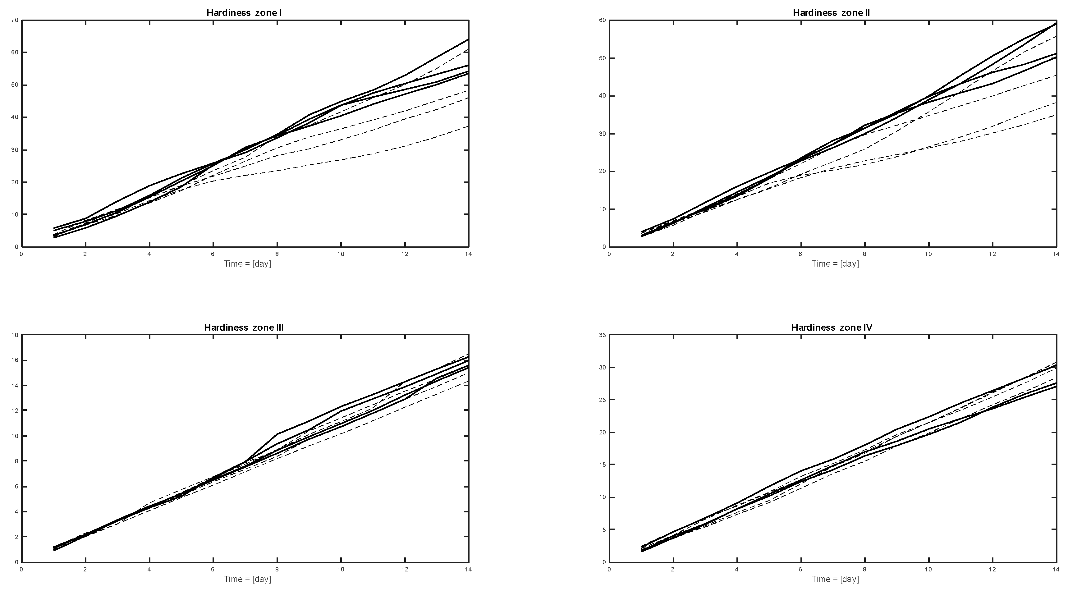
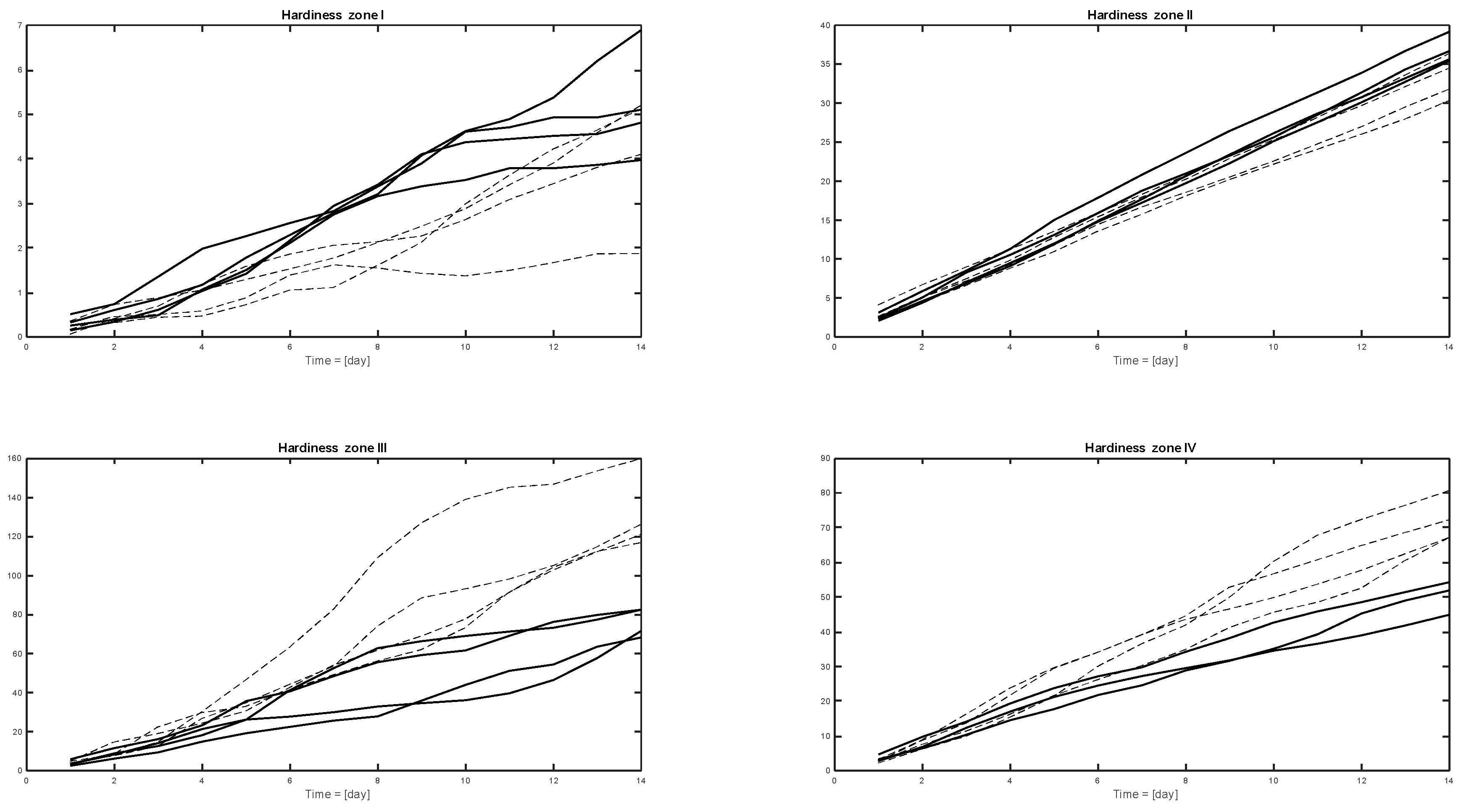
Figure 5.
The cumulative summed feature values (y-axis) generated from weather data of the different hardiness zones. The category 0 data (four years’ data in hardiness zones I, II and III, and three years data in hardiness zone IV) are marked with a solid line and category 1 data (four years in each hardiness zone) with a dashed grey line. The observation period is 14 days, t0 is the beginning of growing season, and the time step is one day (x-axis).

Figure 6.
The cumulative summed feature values (y-axis) generated from weather data of the different hardiness zones. The category 0 data (four years’ data in hardiness zones I, II and III, three years’ data in hardiness zone IV) are marked with a solid line and the category 2 data (four years in each hardiness zone) with a dashed grey line. The observation period is 14 days, t0 is the beginning of growing season, and the time step is one day.

Figure 7.
The cumulative summed feature values (y-axis) for the cases’ reference data vs. category 1 data (above) and reference data vs. category 2 data (below). The weather data used included hardiness zones I–IV.
Figure 7.
The cumulative summed feature values (y-axis) for the cases’ reference data vs. category 1 data (above) and reference data vs. category 2 data (below). The weather data used included hardiness zones I–IV.

Figure 8.
The cumulative summed feature values (y-axis) for the cases’ reference data vs. independent category 2 data. The weather data used included hardiness zones I–IV.
Figure 8.
The cumulative summed feature values (y-axis) for the cases’ reference data vs. independent category 2 data. The weather data used included hardiness zones I–IV.


Table 1.
General information about the data selected for analysis.
| Barley Leaf Area (Percentage), Infected by Net Blotch | <0.5% Category 0 | 0.6–5% Category 1 | >5% Category 2 |
|---|---|---|---|
| Number of Available Datasets (Years) Per Category | |||
| Hardiness zone I | 8 | 5 | 12 |
| Hardiness zone II | 6 | 7 | 8 |
| Hardiness zone III | 6 | 6 | 13 |
| Hardiness zone IV | 3 | 8 | 11 |
Table 2.
Statistical values of the weather data variables at the starting point of the analysis.
| Mean value | ||||||||
| Hardiness zone I | ||||||||
| Beginning of growing season | Sowing time | |||||||
| R [mm] | Tav [°C] | Tmax [°C] | Tmin [°C] | R[mm] | Tav [°C] | Tmax [°C] | Tmin [°C] | |
| Category 0 | 0.5 | 8.8 | 14.8 | 2.6 | 0.9 | 10.0 | 15.3 | 4.4 |
| Category 1 | 0.8 | 7.6 | 13.2 | 2.1 | 1.0 | 11.9 | 17.4 | 6.3 |
| Category 2 | 0.8 | 9.6 | 15.4 | 3.6 | 1.1 | 12.9 | 18.1 | 7.2 |
| Hardiness zone II | ||||||||
| Beginning of growing season | Sowing time | |||||||
| R[mm] | Tav [°C] | Tmax [°C] | Tmin [°C] | R[mm] | Tav [°C] | Tmax [°C] | Tmin [°C] | |
| Category 0 | 0.8 | 7.8 | 13.9 | 1.4 | 1.7 | 9.4 | 15.0 | 3.8 |
| Category 1 | 0.7 | 9.1 | 15.1 | 3.1 | 1.6 | 11.7 | 17.2 | 6.0 |
| Category 2 | 1.4 | 8.6 | 14.5 | 2.4 | 1.8 | 12.8 | 18.1 | 7.2 |
| Hardiness zone III | ||||||||
| Beginning of growing season | Sowing time | |||||||
| R[mm] | Tav [°C] | Tmax [°C] | Tmin [°C] | R[mm] | Tav [°C] | Tmax [°C] | Tmin [°C] | |
| Category 0 | 0.6 | 7.1 | 13.0 | 1.1 | 2.1 | 10.1 | 15.7 | 4.1 |
| Category 1 | 0.9 | 8.4 | 14.6 | 2.3 | 1.8 | 12.0 | 17.8 | 5.9 |
| Category 2 | 1.2 | 9.7 | 15.6 | 3.5 | 2.1 | 11.3 | 16.9 | 5.1 |
| Hardiness zone IV | ||||||||
| Beginning of growing season | Sowing time | |||||||
| R[mm] | Tav [°C] | Tmax [°C] | Tmin [°C] | R[mm] | Tav [°C] | Tmax [°C] | Tmin [°C] | |
| Category 0 | 0.8 | 8.4 | 14.1 | 2.4 | 1.1 | 10.5 | 15.6 | 4.2 |
| Category 1 | 1.1 | 9.5 | 15.3 | 3.4 | 1.3 | 11.4 | 16.8 | 5.7 |
| Category 2 | 1.5 | 8.9 | 14.2 | 3.7 | 2.8 | 11.0 | 15.9 | 6.0 |
| Standard deviation | ||||||||
| Hardiness zone I | ||||||||
| Beginning of growing season | Sowing time | |||||||
| R[mm] | Tav[°C] | Tmax[°C] | Tmin[°C] | R[mm] | Tav[°C] | Tmax[°C] | Tmin[°C] | |
| Category 0 | 1.6 | 3.6 | 4.4 | 3.8 | 2.2 | 3.5 | 4.0 | 4.1 |
| Category 1 | 1.9 | 3.2 | 4.2 | 3.7 | 2.2 | 3.5 | 4.4 | 3.8 |
| Category 2 | 2.4 | 3.7 | 4.1 | 4.6 | 2.2 | 3.5 | 4.4 | 3.8 |
| Hardiness zone II | ||||||||
| Beginning of growing season | Sowing time | |||||||
| R[mm] | Tav [°C] | Tmax [°C] | Tmin [°C] | R[mm] | Tav [°C] | Tmax [°C] | Tmin [°C] | |
| Category 0 | 2.2 | 3.6 | 4.5 | 3.6 | 4.2 | 2.9 | 3.4 | 3.9 |
| Category 1 | 2.4 | 4.2 | 4.7 | 4.7 | 3.3 | 3.8 | 4.7 | 4.1 |
| Category 2 | 3.6 | 3.7 | 4.6 | 3.6 | 3.3 | 3.8 | 4.6 | 3.9 |
| Hardiness zone III | ||||||||
| Beginning of growing season | Sowing time | |||||||
| R[mm] | Tav [°C] | Tmax [°C] | Tmin [°C] | R[mm] | Tav [°C] | Tmax [°C] | Tmin [°C] | |
| Category 0 | 1.4 | 3.0 | 4.1 | 3.4 | 5.7 | 3.5 | 4.2 | 4.2 |
| Category 1 | 2.5 | 3.4 | 4.8 | 3.3 | 3.7 | 4.3 | 5.6 | 3.7 |
| Category 2 | 4.3 | 3.1 | 4.0 | 3.8 | 6.2 | 3.7 | 4.6 | 4.1 |
| Hardiness zone IV | ||||||||
| Beginning of growing season | Sowing time | |||||||
| R[mm] | Tav [°C] | Tmax [°C] | Tmin [°C] | R[mm] | Tav [°C] | Tmax [°C] | Tmin [°C] | |
| Category 0 | 1.8 | 4.0 | 5.3 | 3.5 | 2.5 | 4.6 | 5.6 | 4.5 |
| Category 1 | 2.6 | 3.6 | 4.4 | 3.9 | 2.8 | 3.4 | 4.3 | 3.5 |
| Category 2 | 2.6 | 4.3 | 5.0 | 4.6 | 5.4 | 3.8 | 4.6 | 4.4 |
| Median | ||||||||
| Hardiness zone I | ||||||||
| Beginning of growing season | Sowing time | |||||||
| R[mm] | Tav[°C] | Tmax[°C] | Tmin[°C] | R[mm] | Tav[°C] | Tmax[°C] | Tmin[°C] | |
| Category 0 | 0 | 8.25 | 14.6 | 2.4 | 0 | 9.85 | 14.8 | 4.15 |
| Category 1 | 0 | 7.6 | 13.2 | 2.4 | 0 | 11.15 | 16.7 | 6.45 |
| Category 2 | 0 | 9.05 | 14.6 | 3.9 | 0 | 12.6 | 17.65 | 8.05 |
| Hardiness zone II | ||||||||
| Beginning of growing season | Sowing time | |||||||
| R[mm] | Tav [°C] | Tmax [°C] | Tmin [°C] | R[mm] | Tav [°C] | Tmax [°C] | Tmin [°C] | |
| Category 0 | 0 | 7.7 | 13.5 | 1.55 | 0.1 | 9.5 | 14.9 | 4.45 |
| Category 1 | 0 | 8.75 | 15.25 | 2.85 | 0 | 11.15 | 16.35 | 6.15 |
| Category 2 | 0 | 8.2 | 14.05 | 2.5 | 0.05 | 12.45 | 17.55 | 7.15 |
| Hardiness zone III | ||||||||
| Beginning of growing season | Sowing time | |||||||
| R[mm] | Tav [°C] | Tmax [°C] | Tmin [°C] | R[mm] | Tav [°C] | Tmax [°C] | Tmin [°C] | |
| Category 0 | 0 | 6.85 | 12.9 | 0.75 | 0 | 10.3 | 15.5 | 4.3 |
| Category 1 | 0 | 8.2 | 14.6 | 1.6 | 0 | 11.6 | 16.9 | 5.9 |
| Category 2 | 0 | 9.5 | 15.0 | 3.45 | 0 | 11.4 | 16.95 | 5.2 |
| Hardiness zone IV | ||||||||
| Beginning of growing season | Sowing time | |||||||
| R[mm] | Tav [°C] | Tmax [°C] | Tmin [°C] | R[mm] | Tav [°C] | Tmax [°C] | Tmin [°C] | |
| Category 0 | 0 | 7.7 | 13.3 | 2.1 | 0 | 10.95 | 15.2 | 4.25 |
| Category 1 | 0 | 9 | 14.8 | 3.35 | 0 | 10.9 | 15.9 | 5.85 |
| Category 2 | 0 | 8 | 13.35 | 3.3 | 0.35 | 10.75 | 15.8 | 5.8 |
Table 3.
Results of the statistical feature evaluation.
| The Number of Days When the Null Hypothesis Was Rejected | ||||
|---|---|---|---|---|
| Observation Field | t0 = Beginning of the Growing Season | t0 = Sowing Date | ||
| Category | Category | |||
| 0 vs. 1 | 0 vs. 2 | 0 vs. 1 | 0 vs. 2 | |
| Hardiness zone I | 9 | 11 | 8 | 9 |
| Hardiness zone II | 11 | 11 | 11 | 11 |
| Hardiness zone III | 10 | 9 | 9 | 8 |
| Hardiness zone IV | 10 | 10 | 9 | 9 |
Table 4.
The most suitable features for separating between the reference data (category 0) and category 1 and 2 datasets. The original variables are denoted as a, b, c, and d—namely R, Tav, Tmax, and Tmin.
Table 4.
The most suitable features for separating between the reference data (category 0) and category 1 and 2 datasets. The original variables are denoted as a, b, c, and d—namely R, Tav, Tmax, and Tmin.
| Place of Observations | t0 = Beginning of the Growing Season | |
|---|---|---|
| Category | ||
| 0 vs. 1 | 0 vs. 2 | |
| Hardiness zone I | (a + b)·b | ln(c) + (b)·ln(d) |
| Hardiness zone II | D + b2 | a·d |
| Hardiness zone III | (a·c)/b | d2· b2 |
| Hardiness zone IV | (b + d)/c | (d + a)·d |
© 2020 by the authors. Licensee MDPI, Basel, Switzerland. This article is an open access article distributed under the terms and conditions of the Creative Commons Attribution (CC BY) license (http://creativecommons.org/licenses/by/4.0/).
Share and Cite
MDPI and ACS Style
Ruusunen, O.; Jalli, M.; Jauhiainen, L.; Ruusunen, M.; Leiviskä, K. Advanced Data Analysis as a Tool for Net Blotch Density Estimation in Spring Barley. Agriculture 2020, 10, 179. https://doi.org/10.3390/agriculture10050179
AMA Style
Ruusunen O, Jalli M, Jauhiainen L, Ruusunen M, Leiviskä K. Advanced Data Analysis as a Tool for Net Blotch Density Estimation in Spring Barley. Agriculture. 2020; 10(5):179. https://doi.org/10.3390/agriculture10050179
Chicago/Turabian StyleRuusunen, Outi, Marja Jalli, Lauri Jauhiainen, Mika Ruusunen, and Kauko Leiviskä. 2020. "Advanced Data Analysis as a Tool for Net Blotch Density Estimation in Spring Barley" Agriculture 10, no. 5: 179. https://doi.org/10.3390/agriculture10050179
Note that from the first issue of 2016, this journal uses article numbers instead of page numbers. See further details here.