
Characterisation and Design of Direct Numerical Simulations of Turbulent Statistically Planar Flames


1
Chair of Space Propulsion, Technische Universität München, Boltzmannstraße 15, 85748 Garching, Germany
2
Chair of Space Systems, Technische Universität Dresden, Marschnerstraße 32, 01307 Dresden, Germany
*
Author to whom correspondence should be addressed.
Aerospace 2022, 9(10), 530; https://doi.org/10.3390/aerospace9100530
Submission received: 17 May 2022
/
Revised: 23 August 2022
/
Accepted: 25 August 2022
/
Published: 21 September 2022
(This article belongs to the Special Issue Aerospace Combustion Engineering)
Abstract
:This work aims to provide support for the design of reliable DNSs for statistically planar flames. Improved simulation design strategies are developed. Therefore, design criteria for the simulative domain are discussed. The gained mathematical relations for all of the relevant physical quantities were channelled into a deterministic calculation strategy for mesh features. To choose design parameter values within the mathematical formulations, guidelines were formulated. For less controllable variables, namely the viscosity and Prandtl number, a measurement technique was developed. A new determination strategy to determine characteristic points within the flame front was conducted. In order to present and compare cases with different Prandtl numbers, normalisation of the x-axis of the regime diagram was suggested.
Keywords:
turbulent combustion; premixed flame; DNS; combustion regime; flame brush; flame viscosity1. Introduction
Traditionally, the use of DNSs was restricted to purely academic communities due their prohibitive computational costs. However, their use is very often unavoidable when trying to quantify and understand different phenomena in flow fields. This understanding leads to physical models, which are applied in simulative approaches with lower fidelity [1]. With computational power rising exponentially, the breadth of applications for DNSs is projected to increase in the foreseeable future. New technologies such as quantum computing [2] might accelerate this trend. Alternative to investigation purposes, DNSs serve as training data for ML algorithms. Complex problems with entangled physical interactions such as premixed turbulent flames are predestined for DNS analysis. The current work’s purpose is to present optimisation strategies and limiting factors for designing DNSs with premixed turbulent flames. Despite their simple configurations, these simulations enable various physical phenomena, including detailed structures, turbulence–chemistry interaction (TCI), and anisotropy, to be studied [3,4,5,6,7,8,9,10]. Limited computational power and RAM enforce strict trade-offs regarding simulation parameters and the solution’s fidelity. Careful optimisation processes result in simulations, which target pertinent scientific questions with finite resources. A systematic approach for designing resource-effective DNSs using premixed flames is proposed in the present research. The suitability of the corrections conducted in this work present different levels of relevance depending on the scientific goals behind the simulation. For instance, TCI problems focused on the correct definitions of combustion regimes. Investigations on enthalpy evolution and on how to model it, on the other hand, benefit from discussions on the choice of representative flame characteristic values. However, since this effort was carried out by the authors within their work on space propulsion applications, the operating conditions used here were chosen accordingly, meaning higher Damköhler values at high pressure levels and strong density gradients. The paper is structured as follows:
In the theory section, an overview of all of the important physical relations is derived. In the following section, the conducted work is presented via a thorough discussion of the results. There, mathematical functions required for the calculation of the necessary mesh size depending on a variety of parameters are derived first. Then, a decision strategy for the design parameter within these functions is elaborated. Afterwards, a determination technique that allows the flame characteristic values to be retrieved from within the flame is derived. These values can be applied in the above-mentioned mesh size calculations. Finally, cases with different values are depicted within a regime diagram. In order to improve the comparability between these cases, an adaptive modification of the classical version of a regime diagram [11,12,13,14] is introduced.
2. Theoretical Background
The presented work deals with premixed statistically planar flames, and their characterisation is presented here. Some characterising values (e.g., flame thickness) and dimensionless numbers () have more than one mathematical expression. These definitions are based on common concepts, but they are mathematically adapted according to the research purpose. This circumstance is reflected in this section.
2.1. Laminar Flame Theory
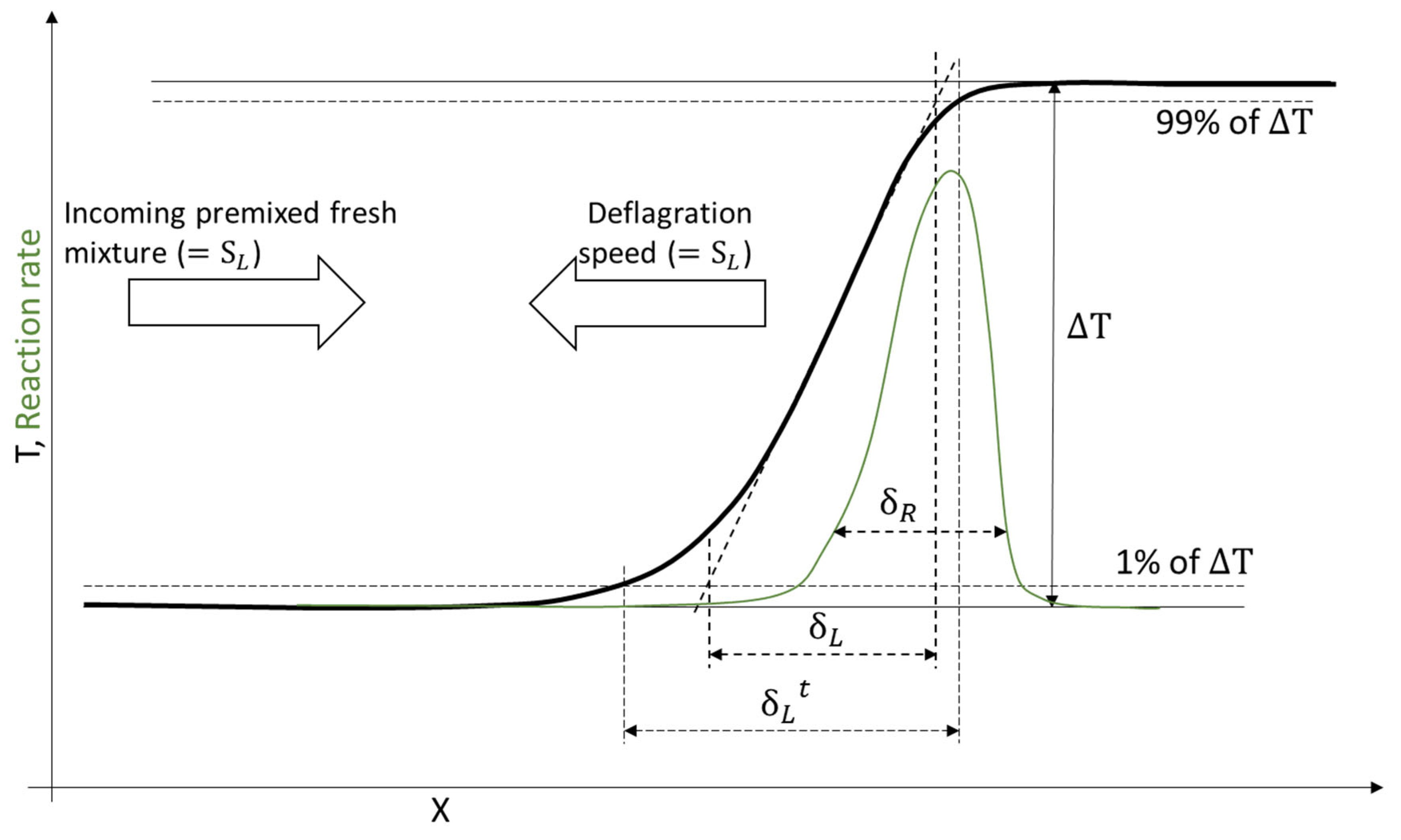
Figure 1 shows a generic temperature distribution through the flame front of a burning low-carbon fuel. is defined as the velocity of the incoming flow, which remains constant. This definition is universal. The laminar flame thickness, however, can be interpreted in many ways. In this work, it is defined by the linearisation of the thermal flame front (). The reason for this is that the thermal gradient of the flame front is the driving force of its impact on the turbulent flow. Alternative definitions are based on empirical relations or on absolute temperature differences () [15].
2.2. Turbulent Flame Theory
For the research on TCI, the time scales of turbulence and reaction are juxtaposed. The universal definitions of the relevant turbulent Damköhler number and the turbulent Karlovitz number are:
The main difference between these two definitions is the correspondence between the turbulent time scales. The Damköhler number is determined according to the turbulent macroscales, and the Karlovitz number is determined according to the microscales. Interpretations of the different time scale statements depend on the literature [11,15]. The definitions used in this work, however, define the time scales as the quotient of the thickness and the speed of the turbulence or flame.
Note that here, u′ is an integral turbulent characteristic according to .
The turbulent Reynolds number was determined according to the characteristic length of the eddies Λ (not the “biggest” eddies). is also an indicator of the ratio of the characteristic length scale to the Kolmogorov length. The Kolmogorov length is also involved in , where it is assumed to be 1.
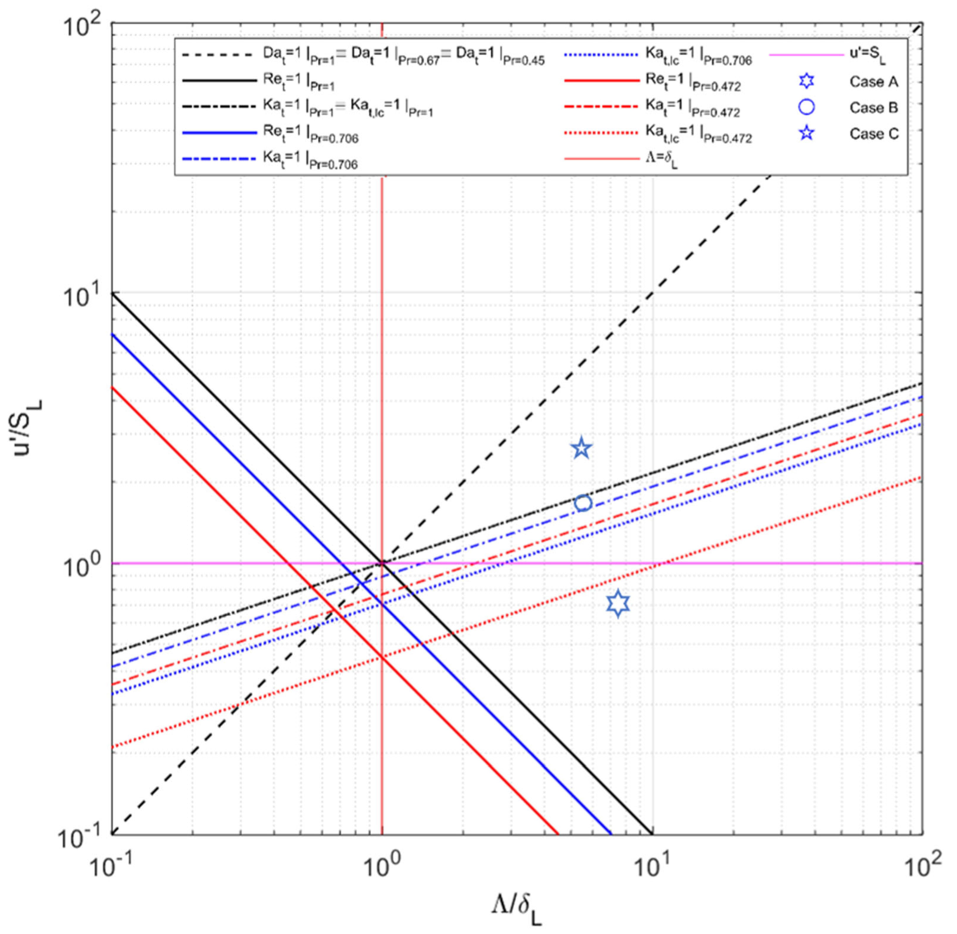
Regime diagrams as proposed by different sources [12,13,14,16,17] visualise different regimes of premixed flames in terms of , and . This way of depiction allows a quick identification of flame features relevant for a respective scientific interest. However, the usually used assumption here is that the Prandtl number is 1. This value can be very misleading, since Prandtl numbers of different gas mixtures at different temperatures and pressures can vary by an order of magnitude. The general way to define the local Prandtl number, especially in flames is in Equation (12), where each value is to be taken from the same local sate of the gas
A juxtaposition of Equations (9) and (12) shows that there are two ways of defining and hence . One way is to use the integral characteristics of the flame front, and the other is to take the values of the local gas. These methods of calculation can result in very different values, as discussed in the following section. This issue is often avoided by equalising with and therefore assuming to be 1 [18,19]. This assumption does not hold for most gases. For example, the characteristic Prandtl number within a CH4-O2 flame under 20 bar is 0.706, where before the reaction, and after the reaction. In case the of a H2-O2 flame, .
The functions in Equations (13)–(16) can be derived by combining the given definitions in Equations (2)–(12) in different ways:
- For the function behind in Equation (13), it is sufficient to rearrange Equation (3).
- The function for is the result of Equation (8) being plugged into Equation (10), leading to . That expression can be rearranged to create Equation (14).
- The function for is derived from Equation (4), where statements from Equations (11) and (6) are plugged, in leading to . Here, Equation (10) and then Equation (8) can be plugged in, resulting in . A simple rearrangement leads to Equation (15).
- For the derivation of , Equation (5) is combined with Equation (6) to create ()/(). Here, the statement from Equation (10) is plugged in, leading to . The insertion of Equation (8) results in Now, Equation (16) can be inferred.
These are the functions behind the isolines in Figure 2. There are various ways to divide the diagram into distinctive regime regions [16,17,20]. These elaborated thresholds are mainly based on the isolines for , , , and . However, in this work, the general treatment of these isolines is discussed. Therefore, the presented version of the regime diagram is reduced to the three essential unity lines of the dimensionless numbers. Any -dependent shift in these unity lines can be easily reproduced for any other value. This way, a shift in any possible regime threshold can be accounted for.
Cases A, B, and C are simulations that were conducted and that are characterised within the regime diagram. Their properties are summarised in Table 1. The underlying decisions about the design parameters of the domain were based on [21,22], as was the design strategy, which is elaborated upon in this work. The results of these simulations serve as the corroboration for the discussions and improvements in Section 3.
2.3. Simulative Setup
The simulation tool that was used was the EBI-DNS [23] solver within the OpenFoam [24,25] environment. The governing equations in this solver were determined according to compressible Navier–Stokes formulation [15]. The conservation of mass and momentum are solved as in Equations (17) and (18), respectively.
The assumption of a Newtonian fluid was made for the stress tensor.
The discretisation schemes are of the second and third orders; thus, the method can be called a quasi-DNS method. It was shown by the creators that for the study of turbulent combustion, low discretisation is an appropriate compromise [26]. Chemical integration was conducted with Cantera algorithms [27] and an averaged transport mixing model [28], which were incorporated into the C++-based environment of the solver. The chemical mechanism of Slavinskaya et al. [29] that was used represents all of the relevant species for near-stochiometric methane–oxygen mixtures at the high pressure levels that occur in different space propulsion applications. It includes 21 species and 97 reactions.
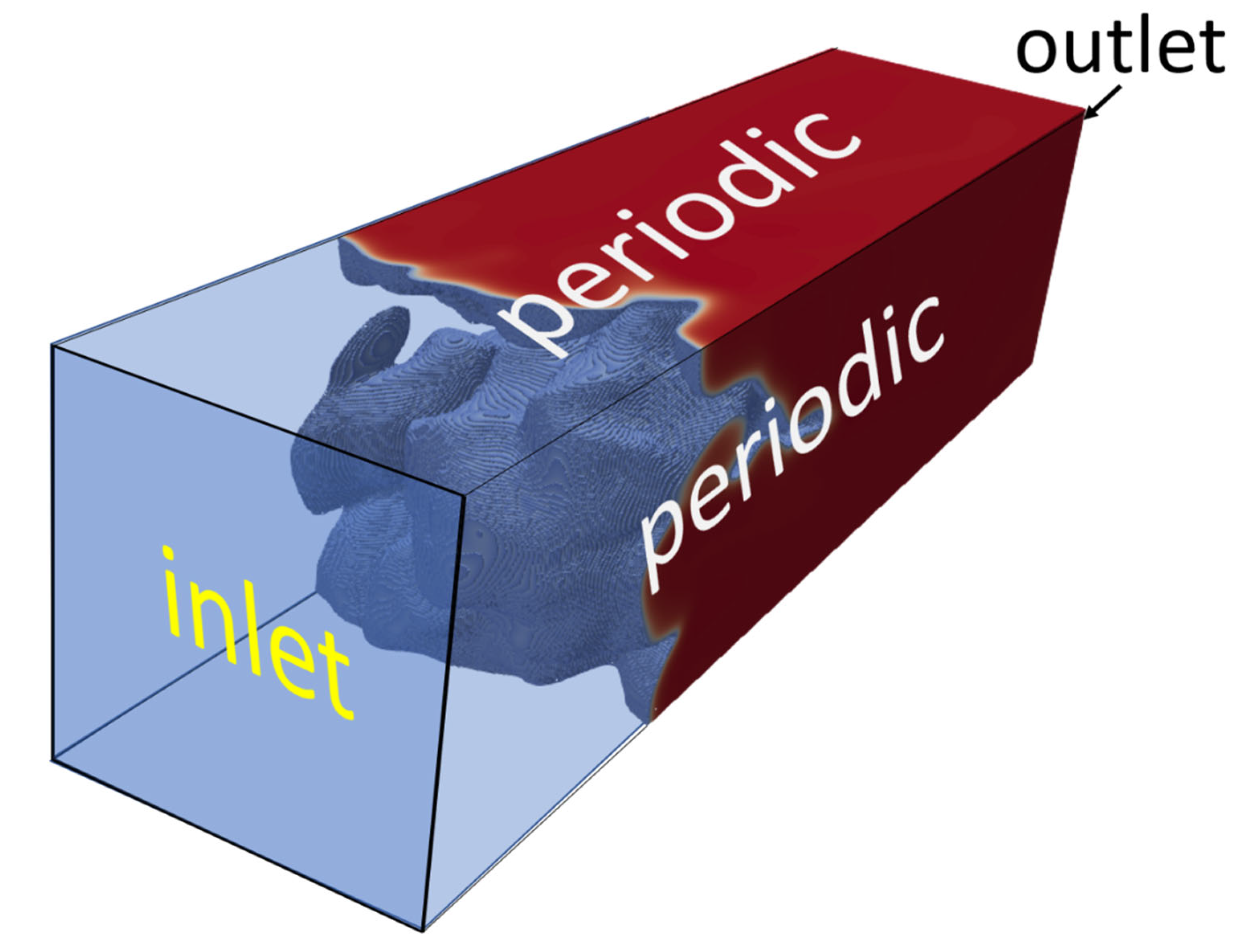
Figure 3 depicts a stationary turbulent flame exposed to an incoming cold premixed turbulent flow. On the left, flow is coming in (“fixedValue” of velocity and pressure), and a moving bulk flow automatically stabilises the flame in the middle of the domain. Synthetic turbulence is patched upon the entering flow. However, it evolves into natural turbulence before reaching the flame brush [22,30]. This natural turbulence corresponds to the widely known HIT-turbulent cascade and is matched by the function in Equation (20) [31]. The production zone, the inertia zone, and the dissipation zone are the typical parts of this type of energy spectrum. Theoretically, this cascade starts at the theoretical wave number of 0. This assumption requires the flame brush to be able to extend infinitely to cover the whole energy spectrum. Nevertheless, the usage of HIT theory in the context of combustion characterisation is currently still a standard approach in the community. Though this issue would be very interesting to research, is not the main focus of this work. The reason for this is that the generic flame configuration treated here avoids introducing relevant anisotropy into the upstream turbulence. The anisotropy after the flame is significant; however, it has only a minor impact on the flame brush.
On the right side of the domain in Figure 3, the flow is exiting the domain. The boundary condition “zeroGradient” offers variable outlet pressure depending on the pressure drop in the system.
Since all side boundaries are “periodic”, this flame can be seen as one-dimensional in macroscopic terms. Therefore, the turbulent flame brush shares features with the 1D-laminar flame front. Such features include the local thickness and local deflagration velocity.
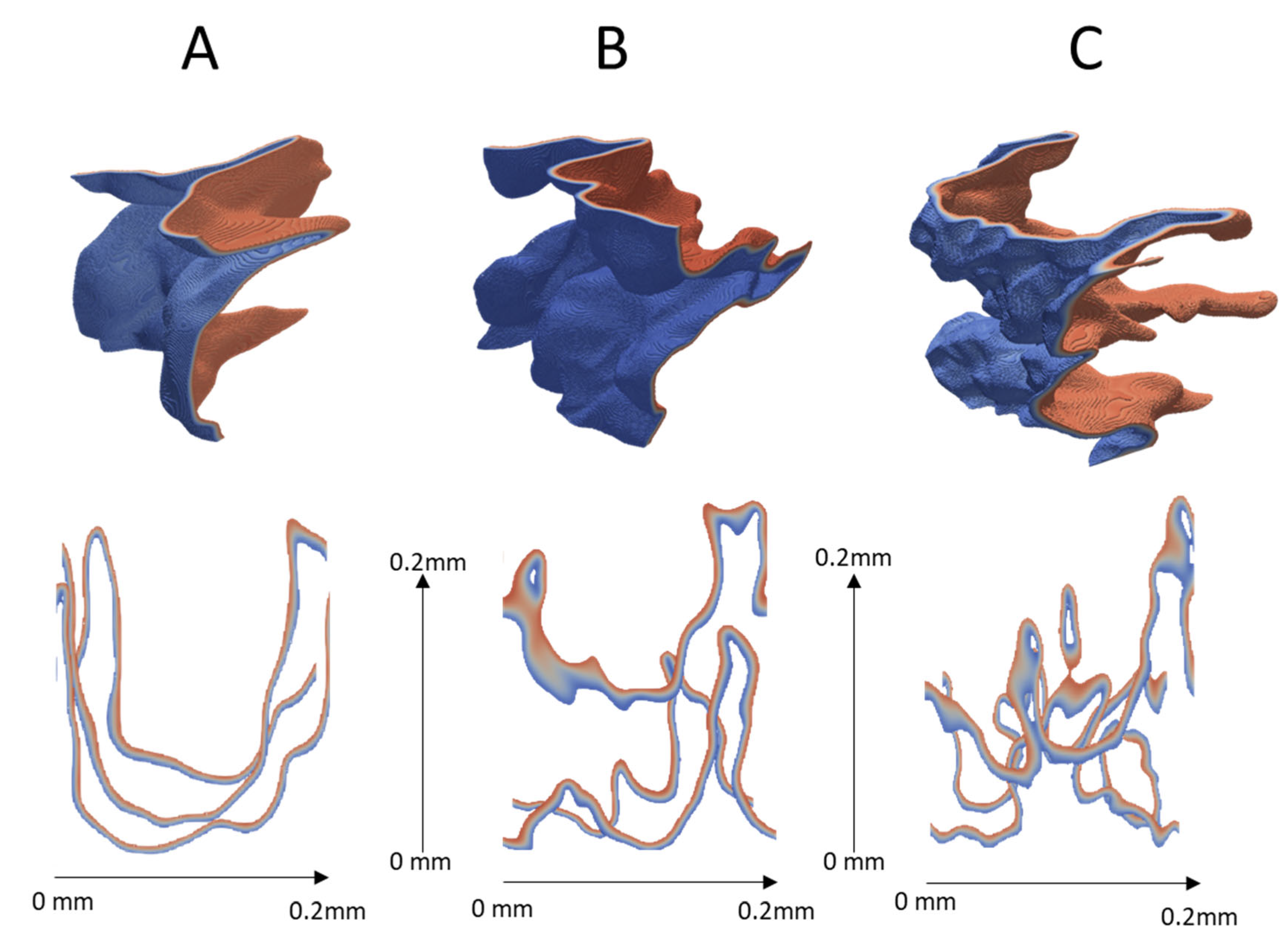
The flame brushes visualised in Figure 4 reveal a known pattern that is distinctive to the respective flame regimes. The length scale of wrinkling depends on the predominancy of the turbulent time scale over the chemical time scale.
As cases A and C are both far away from the threshold of , their optical patterns clearly represent their respective positions in the regime diagram. The closeness of case B to unity makes it difficult to assign it to a distinctive regime.
All of the flame fronts show local chaotic structures. If their DNS results are averaged over 100–200 time steps, they reveal homogeneous flame fronts, as shown in Figure 5. This averaged depiction provides additional characteristics of the flame, such as the turbulent flame brush thickness, as it would appear in an RANS solution. It also becomes obvious that the averaged solution is constantly planar. Only weak deviations in a certain percent range are still noticeable. Hence, the configuration below will be labelled as a “statistically planar flame”.
3. Results and Discussion
This section discusses the crucial impacts on the design of reactive direct numerical simulations (DNS). The focus lies on the vital optimisation of computational resources. This goal is achieved by deriving reproducible mathematical formulations for a cost calculation in Section 3.1. Some quantities used by the equations are design criteria, which are chosen by the user. Accordingly, deterministic rules for the trade-off of these parameter are discussed in Section 3.2. Other less controllable quantities are prevailing flame characteristics (). In order to apply them in the design calculations, correct values have to be determined. Therefore, the measurement technique for reading out characteristic inner flame values has been improved in Section 3.3. Finally, the conducted derivations and improvements are incorporated into the regime diagram. For a better comparability between cases with different thermophysical characteristics, a modification of the diagram is suggested.
3.1. Mathematical Relations of Design Parameters
In this sub-chapter, holistic formulae are created, which enable the calculation of the necessary mesh size from different combinations of design parameters. The following defining parameters can be identified: kinematic viscosity ; laminar flame velocity ; laminar flame thickness ; turbulent Damköhler number ; turbulent Reynolds number ; turbulent Karlovitz number ; turbulent intensity expressed by u′; characteristic turbulent length Λ; flame front resolution ; domain size by the characteristic length of the turbulence ; aspect ratio of the domain ; and mesh size (number of cells in the mesh) . The general form for calculating the necessary mesh size is as stated as in Equation (21). This formulation is based on the information from the turbulent flame, which, in this case, is and or . Together with the flame front resolution, they define the number of cells needed to cover the length of . This value is multiplied by to determine how much the domain will cover in the lateral direction. The resulting value represents the total number of cells in one direction. Raising this value by a power of 3 acquires the number of cells within a cube. This number is finally multiplied with the aspect ratio , which enables the sufficient independence of the flame brush from the inlet and outlet conditions. Since the value of is rarely predetermined, it can be replaced with the relation of better plannable values. This relation, which is shown in Equation (22), results from the combination of Equations (6) and (10):
In this standard form, the inputs of , , , , , , and are needed to calculate . Alternatively, it is possible to replace two values in this list with dimensionless numbers. For example, instead of predefining η and , they can be replaced with dependencies on the desired , , , or . This makes it possible to target particular points in the regime diagram. The mathematical packages needed for this are shown in Equations (23)–(30). Sufficient parameters must be known for either Equation (22), Equations (23)–(25), Equations (26)–(28), or Equations (29) and (30). Any of these combinations provide values for the calculation of the mesh size using Equation (21). Some parameters must be known and others can be decided, as discussed in the following sub-sections. This workflow can be reproduced in different ways as long as the derived mathematical formulations can be closed with enough known values.
Dependence on and :
where
Dependence on and :
where
Dependence on and :
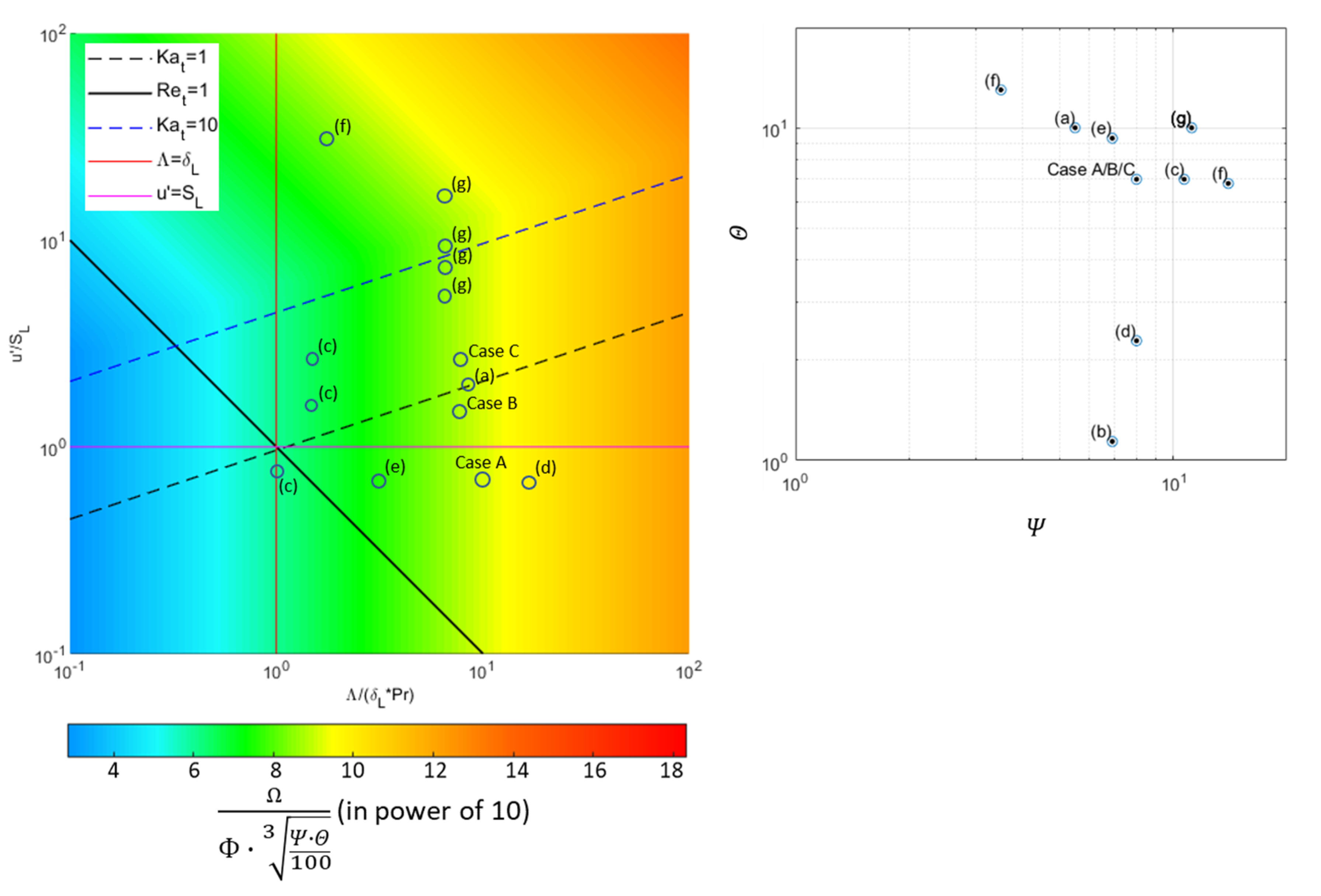
Figure 6 (left) shows the application of these mathematical relations. The colour indicates a third variable in this diagram, next to the x- and y-coordinates. This indicates the mesh size needed for any configuration of chemical and turbulent parameters. Several DNS designs from the literature have been positioned within the diagram. The indicated letters correspond to particular literature according to: (a)[10]; (b)[19]; (c)[21]; (d)[32]; (e)[33]; (f)[34]; (g)[35]. The different positions indicate the design trade-offs made by the respective authors. The colours at each of these positions reveal the mesh size and hence the CPU costs the authors had to accept. The “kink” in the pattern indicates a threshold, where the resolution is determined by the flame front thickness (lower ) instead of the Kolmogorov size (higher ) It becomes obvious that the mesh size increases as and increase and as decreases. This diagram and its colouring are designed to provide maximal universal comparability between the flame under very different conditions. Therefore, the x-axis is normalised, with the shown isolines being almost -independent. The colouring scheme is normalised in such a way that a comparison of different works independent from their respective geometrical features can be conducted. The only non-universal feature of the colouring scheme is the “kink”. Its position is sensitive to different parameters and to the flame front resolution and the Kolmogorov scale in particular. However, it only changes slightly for the shown simulation cases.
It is necessary to state that computational resources are not only dependent on the number of cells but that this is the main driving factor. Empirical data revealed that the relation between the mesh size and the computational costs is slightly non-linear. A refinement of the grid impacts the resources with an exponent of 1.2–1.5. This is due to the smaller time step necessary to keep up a constant maximum CFL number. More necessary time steps drive the CPU costs. This is partially counterbalanced by the faster convergence of the transport equations. There are some factors affecting the choice of the maximum CFL number, which is allowed occur in the domain. The most evident one is the scientifically correct representation of the flow. Even if a CFL above 1 can be established in a stable way, it would partially annihilate the resolution of the finest structures that defined the cell size first. Additionally, highly reactive flow with strong density gradients, such as in the given case, jeopardise the numerical stability significantly. Therefore, the max. CFL number had to be restricted to 0.4. Additional numerical destabilisation factors are forward and backward reaction coefficients above , as calculated from the Arrhenius parameters. In addition to the CFL number, an increased number of intermediate chemical integration steps (100–1000) is used to achieve numerical conversion.
3.2. Trade-Off of Design Parameters
To meet the available computational limitations, priorities must be set in terms of the driving design criteria. For mesh size calculation, the user must choose the values for several driving design quantities. Depending on the individual scientific problem, a trade-off within scientifically valid ranges must be made. In the following section, a best-practice discussion about the choice of appropriate values for , and is conducted.
One common compromise is made between the (flame front resolution) and (ratio of the domain size to characteristic turbulent scale). Both are strong drivers of the mesh size, and both can be subjects to compromises. Depending on the investigated phenomenon, values of 5–64 can be chosen [9,21,36]. In cases where the interior of the flame front is not the object of investigation, a low is sufficient. This is justified because the energy release mainly depends on the chemical scheme and not on the inner flame physics. In cases where there is passive scalar movement or when TCI is to be observed, a of 8–16 is recommended. A higher provides insights into distinctive chemistry and passively advected scalars inside the flame. trade-offs can be applied as well. This quantity has two purposes. It ensures the statistical independence of the turbulence from the periodic boundaries and coverage of a sufficient part of the turbulent energy spectrum [30]. Recommended values for are 2–20. If the focus lies more on the insights regarding the inside of the flame, a high is not necessary. If the turbulent surroundings are prioritised, then the value should ensure a coverage of 80–90% of the integral of the energy cascade. This represents a particular challenge for TCI research since here, the turbulent field as well as the flame structures are observed. Figure 6 (right) depicts the distribution of several simulations from the literature in terms of this trade-off. These examples have either a high flame front resolution or a high domain ratio to characterise the turbulence scale, but seldomly both, as this would exceed the computational resources available in most scientific institutions.
A further adaption parameter is the aspect ratio (). For this, values between 2 and 4 are reasonable. It can be influenced by the turbulence initialisation strategy. If the synthetic turbulence is being injected, it needs time to evolve into natural turbulence [30]. This time is provided by a greater distance between the inlet and the flame brush. If this evolution process is outsourced [10], then a shorter domain can be sufficient. Additionally, independence of the flame from the inlet and outlet must be provided. Depending on the regime, values for bigger than even 4 can become necessary. It should be considered that the computational costs are not linear to the mesh size, as a smaller cell size leads to smaller time steps and hence the need for more time steps for the same flow time. Additionally, the choice of the size of the chemical mechanism influences the calculation time. This influence becomes stronger with smaller cells, as the convergence time of the momentum equation approximates the convergence time of the species transport equations. Furthermore, mechanisms that produce very high reaction coefficients impair the convergence of the reaction solver.
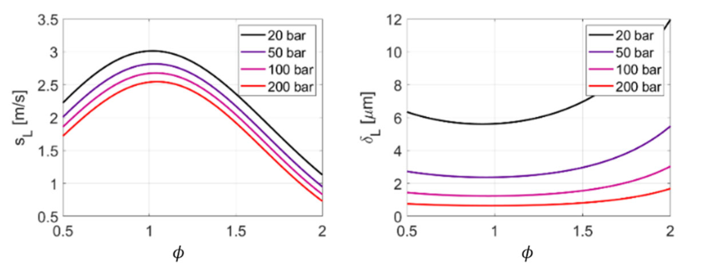
Besides varying the turbulent characteristics of the incoming flow, the chemical time scale can be adapted. It can be matched to a particular application or can be used to control the flame regime. Therefore, the initial conditions, , , or , can be changed [22,37]. An example is shown in Figure 7. More information about the potential of these conditions to serve as a regulator is provided in the general literature [22,29,38].
3.3. Definition of a Representative Point for Characteristic Flame Properties
Besides the design parameters, which are controlled by the user, the resource calculation also includes less controllable qualities, such as . They directly regulate the calculation of and hence, the classification of the flame behaviour. According to the derivations in Equations (2)–(12), all of the flow and flame values should be taken from within the flame front. However, for the turbulence characteristics, it has become a scientific standard to make the measurements in the unburned gas right before the flame brush [19,39]. The reason for this is that making measurements within the flame is very difficult. The evolution of turbulence throughout the flame is strongly non-linear and has a very complex general definition [8]. It can be argued that for some purposes, such as for the investigation of large-scale TCI, this simplification is justified. For the investigation of small-scale TCI, it might be less justified. Measurements taken from isosurfaces within the flame are elegantly presented in [21,22]. However, according to a strict interpretation of the derivations conducted above, all of the values must be retrieved from within the flame. Since the flow properties change significantly throughout the flame front, a characteristic position must be determined as a representative “average”. The choice of the position of such a point has an impact on the sensitive representative flame properties it provides.
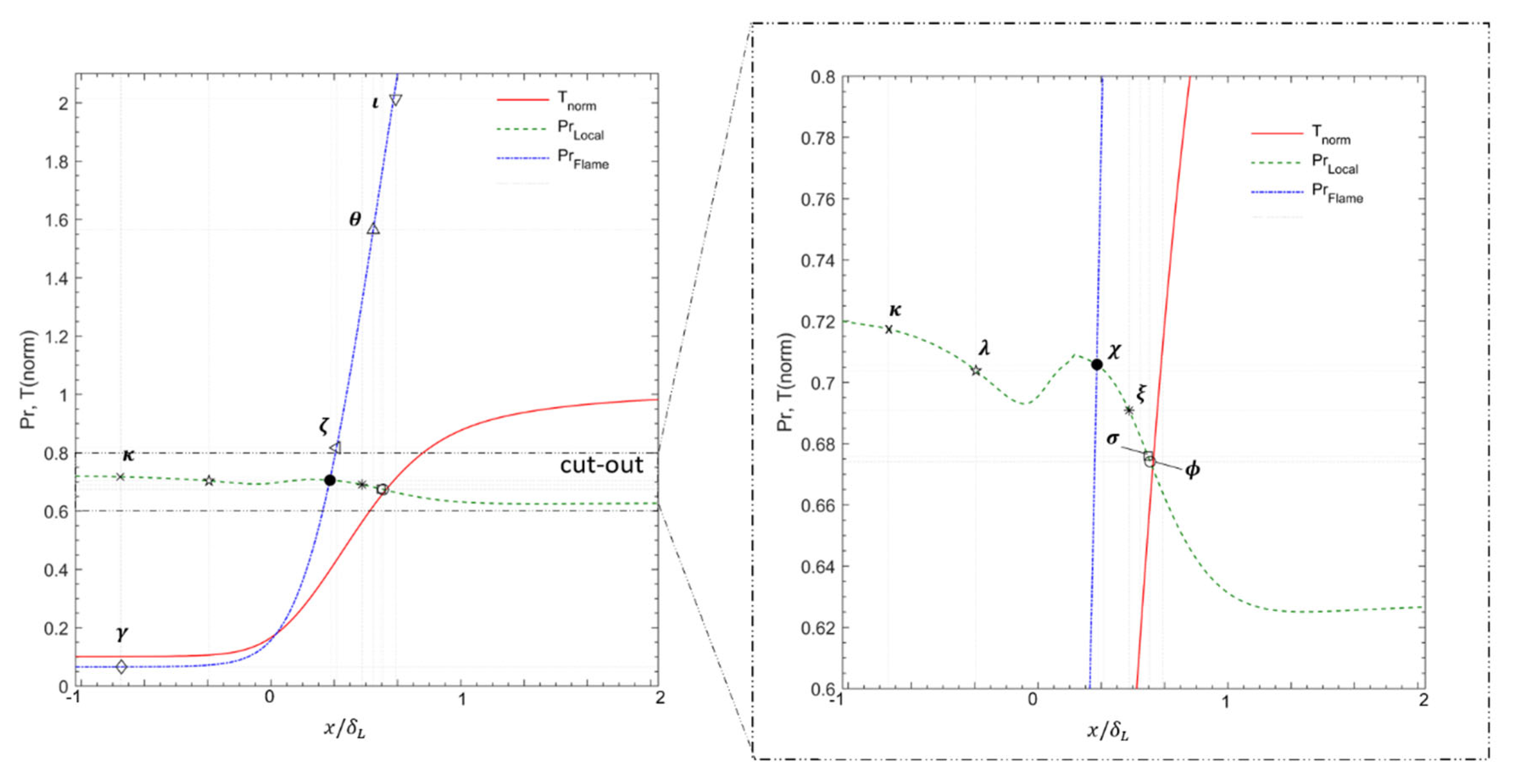
In Table 2, possible choices for the determination of a representative of a statistically planar flame are discussed. They are visualised in Figure 8. The resulting point is described in terms of the and also represents the viscosity at the particular point in the flame front. The first four points are calculated by applying Equation (9) to calculate . According to this integral formulation, the only location-specific variable is the very volatile kinematic viscosity .
In point , the viscosity is taken from the fresh reactants, as also seen in [32,40,41]. This leads to a non-representative value of 0.066. For and , the viscosity throughout the whole flame front is averaged and Favre-averaged, respectively. The resulting values of and are very different and hence represent very different points in the flame front. Hence, the corresponding values are very different as well. Point represents a middle value between the of the reactants and products. Additionally, the resulting number also exceeds a reasonable range.
Subsequent points repeat previous techniques; however, they repeat in terms of the local formulation of from Equation (12). Point represents the most common simplification, where the of the reactants is used [33,42]. In , , and , the local values throughout the flame are calculated as the average, Favre-average, and the middle value, respectively. An alternative option states point , which is at a particular position where the temperature reaches the autoignition temperature. All of the points from to provide similar and reasonable values, with a deviation of 6.3%. However, they are positioned far from each other. Hence, if any other quantity, such as the viscosity value, was to be retrieved from them, the values would strongly vary.
Point is the only point in the flame front that satisfies the universal definition of from Equation (12) as well as the integral definition from Equation (9). Specifically, the latter one is required to be met, as it takes part in the derivation of the functions in the regime diagram. It is suggested that this condition states the most universal definition for a characteristic point in the flame. Viscosity and other values at point can be seen as “characteristic flame values”. Furthermore, an isosurface in the turbulent flame brush created from that condition can be used for purposes such as flame modelling.
The extent to which the determination of the flame characteristic can be demonstrated with DNSs is presented in this work. (Equation (7)) was applied on Equations (29) and (30) and consequently on Equations (21) and (22). was assumed to be either 1 (general simplification) or 0.706 (point ). Additionally, a of 80.5 and a of 0.87 (Table 1) is aimed for in case A. leads to a mesh size of 1710 cells, and leads to a mesh size of 1010 cells and hence a factor of 1.7. This demonstrates how a slight misassumption of can cause a significant miscalculation of computational resources.
3.4. Adaption of the Regime Diagram
The correct consideration of flame characteristic values such as and hence help to not only calculate the computational costs but also to position the simulation case within the regime diagram. However, a distribution of cases with different values in the same regime diagram leads to misleading conclusions about their positions relative to each other and relative to the regime thresholds. This is revealed in Figure 2, where the isolines for , , , and for , (CH4/O2), and (H2/O2) are shown. A shift in the isolines of , , and due to the non-unity of is observable. Only the isoline of stays untouched by the change in . This behaviour is supported by the corresponding Equations (13)–(16). Comparisons with respect to can be conducted without considering different values. However, comparisons in terms of , , or suffer from possible strong deviations in the values between the cases. A stochiometric O2/H2 mixture at 20 bar and at an initial temperature of 350 K results in a of within the flame front. However, fuels with long C-Chains can create a fame with a characteristic that is far above 1 (e.g., gaseous octane–oxygen mixture at 200 bar, = 1.3–1.5). To be able to compare flame brushes at different values, a strategy for the adaption of the regime diagram is derived in this sub-section.
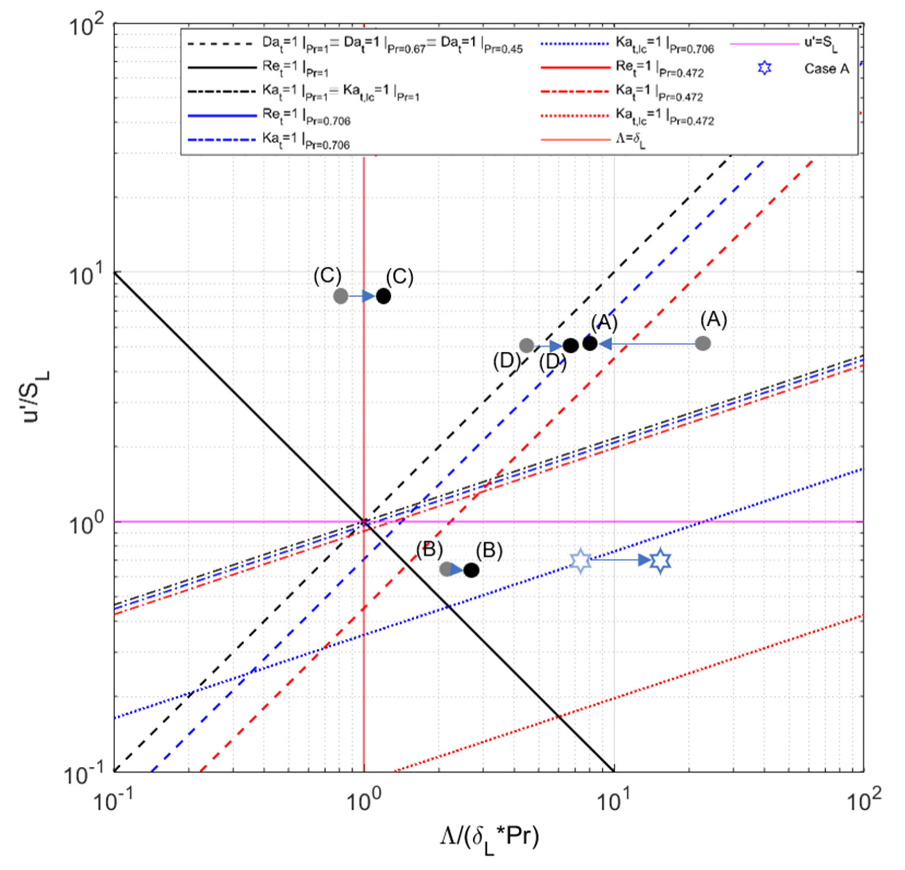
Here, the axes normalise the way that , or becomes -independent. From Equations (13)–(16), the modified functions in Equations (31)–(42) can be derived. There, the definitions for the x- and y-axes are indicated. These derivations follow a common rule, where additional values are introduced to the equation in different ways. For example, Equation (13) becomes Equation (31) by adding the fraction to the equation. The in the numerator is added to the x variable, while the in the denominator stays outside. The same step has been applied to derive Equations (32)–(34). For Equations (35)–(38), the added fraction is and for Equations (39)–(42), it is .
Other added fractions are for the derivation of Equations (35)–(38). As an example, the diagram corresponding to Equations (39)–(42) is shown Figure 9. Also here, the indicated letters correspond to particular literature according to: (A)[19]; (B)[33]; (C)[43]; (D)[35]. As the underlying formulae indicate, the size of the shift in the isolines is independent from their iso-values. However, the shift is very different, depending on the modification of the x-axis. The shown version stands out, as here, the shift in the isoline is minor, and the isoline is stable. This enables comparisons in terms of both criteria. The -dependent shift in the isoline for on the other side is much stronger than in the original regime diagram in Figure 2. To counteract this, the corrections in Equations (35)–(38) can be applied instead. The discussed corrections can be applied graphically or mathematically. In any case, they allow the right association of the flame characteristic parameters ( with the dimensionless numbers (.
independent from Pr:
independent from Pr:
independent from Pr:
4. Conclusions
This work delivers sufficient information to design DNSs of premixed flames as a balanced compromise between compliance with scientific standards and the expenditure of computational resources.
To calculate the mesh size and, subsequently, the computational resources of a DNS for statistically planar flames, design criteria are derived (Equation (21)). Here, a limited number of variables play a role: By knowing eight of them, the rest can be determined. This calculation is deterministic in any direction.
This list contains the freely controllable variables and the partially controllable quantities. The choice of their values is the result of trade-off considerations. Accordingly, rules are formulated, and reasonable ranges are identified. An important compromise must be found between (flame front resolution) and (ratio of the domain size to the characteristic turbulence scale). Depending on whether the investigated phenomena are hidden in the fame front layers or in the large-scale turbulence around it, values of 5–64 for and of 2–20 for can be chosen. For (aspect ratio), values of 2–4 are usually sufficient. The higher the quality of the injected turbulence, the faster it reaches a natural state, and the smaller the aspect ratio can be. (laminar flame velocity) and (laminar flame thickness) can be indirectly controlled by the environmental conditions. These conditions are the mixture ratio, pressure, and initial temperature as well as the choice of the reactants. Depending on the purpose of the investigation and the freedom of choice for the user, and can be deliberately changed to reach the relevant combustion regimes.
Less controllable parameters in the cost calculation of DNS combustion simulations are and thus , which once again impacts . An optimised strategy for the retrieval of these flame front characteristic values was developed. The resulting “average” point within the flame front can be seen as the most universal way to retrieve the flame’s representative quantities. This point, however, can be sensitive to different factors. One of them is the concentration of hydrogen and hence the mass diffusion as well as the counter gradients in the profile. The investigation of this sensitivity can benefit scientific endeavours towards close analysis of inner flame statistics [21,44,45].
The improved determination of the flame characteristic is presented in regime diagrams for different cases. In order to make these cases easier to compare, modification of the x-axis of the regime diagram is suggested. Depending on the correction, either the or isolines become -independent. This way, cases with different values can be visualised within the same diagram and in the correct positions.
Author Contributions
Conceptualisation, A.S., D.M. and O.H.; methodology, A.S. and D.M.; software, D.S.; validation, A.S. and D.M.; formal analysis, O.H. and M.T.; investigation, A.S. and D.M.; resources, O.H. and M.T.; data curation, D.S., O.H. and M.T.; writing—original draft preparation, A.S.; writing—review and editing, D.M. and O.H.; visualisation, A.S.; supervision, O.H. and M.T. All authors have read and agreed to the published version of the manuscript.
Funding
This research was funded by the scholarship from the Ernst-Ludwig-Ehrlich Scholarship Foundation.
Institutional Review Board Statement
Not applicable.
Informed Consent Statement
Not applicable.
Data Availability Statement
Not applicable.
Acknowledgments
The authors thank the computational centre for providing the computational resources for performing the numerical simulations and for their analysis. Special thanks are extended to Martin Ohlerich for his support with the operation of OpenFoam. This paper has benefited from the valuable comments and advice from Andrei Lipatnikov, to whom the authors are extremely grateful.
Conflicts of Interest
The authors declare no conflict of interest. The funders had no role in the design of the study; in the collection, analyses, or interpretation of data; in the writing of the manuscript; or in the decision to publish the results.
Nomenclature
| Latin: | |
| Heat capacity at constant pressure | |
| Damköhler number | |
| Karlovitz number | |
| Turbulent kinetic energy | |
| Molecular Prandtl number | |
| Pressure | |
| Reynolds number | |
| Flame front propagation velocity | |
| Temperature | |
| Time | |
| Velocity | |
| Turbulent fluctuations | |
| X | Molar Fraction |
| Indices | |
| Average between reactants and products | |
| Burned | |
| Chemical | |
| char | Characteristic |
| Initial | |
| Laminar | |
| Length-scale | |
| max | Maximum |
| Turbulence | |
| Unburned | |
| Based on the characteristic length of eddies | |
| Based on the Kolmogorov scale | |
| s | Species index |
| Greek: | |
| Thermal diffusivity | |
| Empirical constant for the Karman spectrum. Usually, it equals 2.7. | |
| Flame front thickness | |
| Flame front thickness based on the turbulence | |
| Flame front thickness based on the reaction zone | |
| Dissipation | |
| Kolmogorov scale | |
| Domain size divided by characteristic length of eddies | |
| Wave number (=1/wave length) | |
| Characteristic length of eddies | |
| Heat conductivity | |
| Molecular viscosity | |
| Density | |
| Time scale | |
| Aspect ratio | |
| ϕ | Equivalence ratio |
| Flame front resolution | |
| Mesh size (=number of cells) | |
| Abbreviations: | |
| DNS | Direct numerical simulation |
| HIT | Homogeneous isotropic turbulence |
| TCI | Turbulence–chemistry interaction |
| ML | Machine learning |
| TKE | Turbulent kinetic energy |
| RAM | Random-access memory |
References
- Chakraborty, N.; Katragadda, M.; Cant, R.S. Statistics and Modelling of Turbulent Kinetic Energy Transport in Different Regimes of Premixed Combustion. Flow Turbul. Combust. 2011, 87, 205–235. [Google Scholar] [CrossRef]
- Cao, Y.; Daskin, A.; Frankel, S.; Kais, S. Quantum Circuit Design for Solving Linear Systems of Equations. Mol. Phys. 2012, 110, 1675–1680. [Google Scholar] [CrossRef]
- Kassem, H.I.; Saqr, K.M.; Aly, H.S.; Sies, M.M.; Wahid, M.A. Implementation of the eddy dissipation model of turbulent non-premixed combustion in OpenFOAM. Int. Commun. Heat Mass Transf. 2011, 38, 363–367. [Google Scholar] [CrossRef]
- Lewandowski, M.; Pozorski, J. Assessment of turbulence-chemistry interaction models in the computation of turbulent non-premixed flames. J. Phys. Conf. Ser. 2016, 760, 012015. [Google Scholar] [CrossRef]
- Ertesvåg, I. Analysis of Some Recently Proposed Modifications to the Eddy Dissipation Concept (EDC). Mol. Phys. 2019, 192, 1108–1136. [Google Scholar] [CrossRef]
- Arndt, C.; Meier, W. Influence of Boundary Conditions on the Flame Stabilization Mechanism and on Transient Auto-Ignition in the DLR Jet-in-Hot-Coflow Burner. Flow Turbul. Combust. 2019, 102, 973–993. [Google Scholar] [CrossRef]
- Magnussen, B. On the structure of turbulence and a generalized eddy dissipation concept for chemical reaction in turbulent flow. In Proceedings of the 19th Aerospace Sciences Meeting, St. Louis, MO, USA, 12–15 January 1981. [Google Scholar] [CrossRef]
- Chakraborty, N. Influence of Thermal Expansion on Fluid Dynamics of Turbulent Premixed Combustion and Its Modelling Implications. Flow Turbul. Combust. 2021, 106, 753–848. [Google Scholar] [CrossRef]
- Towery, C.A.Z.; Poludenko, A.; Urzay, J.; O’Brien, J.; Ihme, M.; Hamlington, P.E. Spectral kinetic energy transfer in turbulent premixed reacting flows. Phys. Rev. 2016, 93, 053115. [Google Scholar] [CrossRef]
- Wang, Z.; Abraham, J. Effects of Karlovitz number on turbulent kinetic energy transport in turbulent lean premixed methane/air flames. Phys. Fluids 2017, 29, 085102. [Google Scholar] [CrossRef]
- Peters, N. Combustion Theory; CEFRC Summer School: Princeton, NJ, USA, 2010. [Google Scholar]
- Borghi, R.; Escudie, D. Assessment of a Theoretical Model of Turbulent Combustion by Comparison with a Simple Experiment. Combust. Flame 1984, 56, 149–164. [Google Scholar] [CrossRef]
- Peters, N. The turbulent burning velocity for large-scale and small-scale turbulence. J. Fluid Mech. 1999, 384, 107–132. [Google Scholar] [CrossRef]
- Libby, P.A.; Williams, F.A. Turbulent Reacting Flows; Academic Press: New York, NY, USA, 1994. [Google Scholar]
- Poinsot, T.; Veynante, D. Theoretical and Numerical Combustion; RT Edwards, Inc.: Morningside, Australia, 2001; ISBN 1-930217-10-2. [Google Scholar]
- Skiba, A.; Wabel, T.; Carter, C.; Hammack, S.; Temme, J.; Driscoll, J. Premixed flames subjected to extreme levels of turbulence part I: Flame structure and a new measured regime diagram. Combust. Flame 2017, 189, 407–432. [Google Scholar] [CrossRef]
- Drsicoll, J.; Chen, J.H.; Skiba, A.; Carter, C.D.; Hawkes, E.R.; Wang, H. Premixed Flames Subjected to Extreme Turbulence: Some Questions and Recent Answers. Prog. Energy Combust. Sci. 2020, 76, 100802. [Google Scholar] [CrossRef]
- Sabelnikov, V.; Lipatnikov, A.N.; Nishiki, S.; Hasegawa, T. Investigation of the influence of combustion-induced thermal expansion on two-point turbulence statistics using conditioned structure functions. J. Fluid Mech. 2019, 867, 45–76. [Google Scholar] [CrossRef]
- Lipatnikov, A.; Chomiak, J.; Sabelnikov, V.; Nishiki, S.; Hasegawa, T. A DNS study of the physical mechanisms associated with density ratio influence on turbulent burning velocity in premixed flames. Combust. Theory Model. 2018, 22, 131–155. [Google Scholar] [CrossRef]
- Im, H.G.; Pal, P.; Wooldridge, M.S.; Mansfield, A.B. A Regime Diagram for Autoignition of Homogeneous Reactant Mixtures with Turbulent Velocity and Temperature Fluctuations. Combust. Sci. Technol. 2015, 187, 1263–1275. [Google Scholar] [CrossRef]
- Martínez-Sanchis, D.; Sternin, A.; Tagscherer, K.; Sternin, D.; Haidn, O.; Tajmar, M. Interactions Between Flame Topology and Turbulent Transport in High-Pressure Premixed Combustion. Flow Turbul. Combust. 2022. [Google Scholar] [CrossRef]
- Martinez, D. A Flame Control Method for Direct Numerical Simulations of Reacting Flows in Rocket Engines. Master’s Thesis, Technical University of Munich, Munich, Germany, 2020. [Google Scholar]
- Zhang, F.; Bonart, H.; Zirwes, T.; Habisreuther, P.; Bockhorn, H.; Zarzalis, N. Direct Numerical Simulation of Chemically Reacting Flows with the Public Domain Code OpenFOAM. In High Performance Computing in Science and Engineering; Springer: Cham, Switzerland, 2015; Volume 14. [Google Scholar] [CrossRef]
- Weller, H.; Tabor, G.; Jasak, H.; Fureby, C. Tensorial Approach to Computational Continuum Mechanics using Object-Oriented Techniques. Comput. Phys 1998, 12, 620–631. [Google Scholar] [CrossRef]
- Weller, H.; Tabor, G.; Jasak, H.; Fureby, C. OpenFOAM; OpenCFD: Bracknell, UK, 2017. [Google Scholar]
- Zirwes, T.; Zhang, F.; Habisreuther, P.; Hansinger, M.; Bockhorn, H.; Pfitzner, M.; Trimis, D. Quasi-DNS dataset of a piloted flame with inhomogeneous inlet conditions. Flow Turbul. Combust. 2020, 104, 997–1027. [Google Scholar] [CrossRef]
- Cantera Developers, Documentation of the Cantera Solvers. Available online: https://cantera.org/science/flames.html (accessed on 18 November 2021).
- Kee, R.; Coltrin, M.; Glarborg, P. Chemically Reacting Flow: Theory and Practice; Wiley & Sons Ltd: Hoboken, NJ, USA, 2017; ISBN 978-1-119-18487-4. [Google Scholar]
- Slavinskaya, N.; Abbasi, M.; Starcke, J.H.; Haidn, O. Methane Skeletal Mechanism for Space Propulsion Applications. In Proceedings of the 52nd AIAA/SAE/ASEE Joint Propulsion Conference, Salt Lake City, UT, USA, 25–27 July 2016. [Google Scholar] [CrossRef]
- Martinez-Sanchis, D.; Sternin, A.; Sternin, D.; Haidn, O.; Tajmar, M. Analysis of periodic synthetic turbulence generation and development for direct numerical simulations applications. Phys. Fluids 2021, 33, 125130. [Google Scholar] [CrossRef]
- Von Kármán, T. Progress in the Statistical Theory of Turbulence. Proc. Natl. Acad. Sci. USA 1948, 34, 530–539. [Google Scholar] [CrossRef]
- Klein, M.; Herbert, A.; Kosaka, H.; Böhm, B.; Dreizler, A.; Chakraborty, N.; Papapostolou, V.; Im, H.G.; Hasslberger, J. Evaluation of Flame Area Based on Detailed Chemistry DNS of Premixed Turbulent Hydrogen-Air Flames in Different Regimes of Combustion. Flow Turbul. Combust. 2019, 104, 403–419. [Google Scholar] [CrossRef]
- Lipatnikov, A.N.; Sabelnikov, V.A.; Nishiki, S.; Hasegawa, T. A direct numerical simulation study of the influence of flame-generated vorticity on reaction-zone-surface area in weakly turbulent premixed combustion. Phys. Fluids 2019, 31, 055101. [Google Scholar] [CrossRef]
- Trivedi, S.; Cant, R.S. Turbulence Intensity and Length Scale Effects on Premixed Turbulent Flame Propagation. Flow Turbul. Combust 2021, 109, 101–123. [Google Scholar] [CrossRef]
- Keil, S.; Klein, N.; Chakraborty, N. Sub-grid Reaction Progress Variable Variance Closure in Turbulent Premixed Flames. Flow Turbul. Combust 2021, 106, 1195–1212. [Google Scholar] [CrossRef]
- Poludenko, A.; Oran, E.S. The interaction of high-speed turbulence with flames: Global properties and internal flame structure. Combust. Flame 2010, 157, 995–1011. [Google Scholar] [CrossRef]
- Liao, S.Y.; Jiang, D.M.; Cheng, Q. Determination of laminar burning velocities for natural gas. Fuel 2004, 83, 1247–1250. [Google Scholar] [CrossRef]
- Konnov, A.; Mohammad, A.; Kishore, V.; Kim, N.; Prathap, C.; Kumar, S. A comprehensive review of measurements and data analysis of laminar burning velocities for various fuel + air mixtures. Prog. Energy Combust. Sci. 2018, 68, 197–267. [Google Scholar] [CrossRef]
- Bobbitt, B.; Blanquart, G. Vorticity isotropy in high Karlovitz number premixed flames. Phys. Fluids 2016, 28, 105101. [Google Scholar] [CrossRef]
- Whitmann, S.; Towery, C.; Poludenko, A.; Hamlington, E. Scaling and collapse of conditional velocity structure functions in turbulent premixed flames. Proc. Combust. Inst. 2019, 37, 2527–2535. [Google Scholar] [CrossRef]
- Lipatnikov, A.N.; Sabelnikov, V.A.; Poludenko, A. Assessment of a transport equation for mean reaction rate using DNS data obtained from highly unsteady premixed turbulent flames. Int. J. Heat Mass Transf. 2019, 134, 398–404. [Google Scholar] [CrossRef]
- Lipatnikov, A.N.; Sabelnikov, V.A.; Nikitin, N.V.; Nishiki, S.; Hasegawa, T. Analysis of synthetic turbulence generation and development for direct numerical simulations applications. Flow Turbul. Combust. 2021, 33, 125130. [Google Scholar] [CrossRef]
- Bougrine, S.; Richard, S. Fuel Composition Effects on Flame Stretch in Turbulent Premixed Combustion: Numerical Analysis of Flame-Vortex Interaction and Formulation of a New Efficiency Function. Flow Turbul. Combust 2014, 93, 259–281. [Google Scholar] [CrossRef]
- Martinez, D.; Banik, S.; Sternin, A.; Sternin, D.; Haidn, O.; Tajmar, M. Analysis of Turbulence Generation and Dissipation in Shear Layers of Methane-Oxygen Diffusion Flames using Direct Numerical Simulations. Phys. Fluids 2022, 34, 045121. [Google Scholar] [CrossRef]
- Lipatnikov, A.; Sabelnikov, V.; Hernández-Pérez, F.; Song, W.; Im, H.G. A priori DNS study of applicability of flamelet concept to predicting mean concentrations of species in turbulent premixed flames at various Karlovitz numbers. Combust. Flame 2020, 222, 370–382. [Google Scholar] [CrossRef]
Figure 1.
Generic stationary laminar flame front, including different definitions of flame thickness. Here, “reaction rate” is defined as the sum of the absolute values of the time derivatives of all of the present species’ molar fractions ().
Figure 1.
Generic stationary laminar flame front, including different definitions of flame thickness. Here, “reaction rate” is defined as the sum of the absolute values of the time derivatives of all of the present species’ molar fractions ().

Figure 2.
Regime diagram for premixed flames with traditionally defined axes. The different colours indicate a shift in -dependent isolines. The dashed lines differentiate between the different dimensionless numbers. To provide examples of how the diagram is used, three simulation cases are positioned inside.

Figure 3.
Central perspective of a general DNS of a turbulent flame brush.

Figure 4.
Three-dimensional depictions and two-dimensional slices (three each) of flame fronts from three DNS-simulated premixed combustion cases (A–C). The slices show the inner patterns. The colour range for filtering the flame fronts is from 1000 K (blue) to 3000 K (red).
Figure 4.
Three-dimensional depictions and two-dimensional slices (three each) of flame fronts from three DNS-simulated premixed combustion cases (A–C). The slices show the inner patterns. The colour range for filtering the flame fronts is from 1000 K (blue) to 3000 K (red).

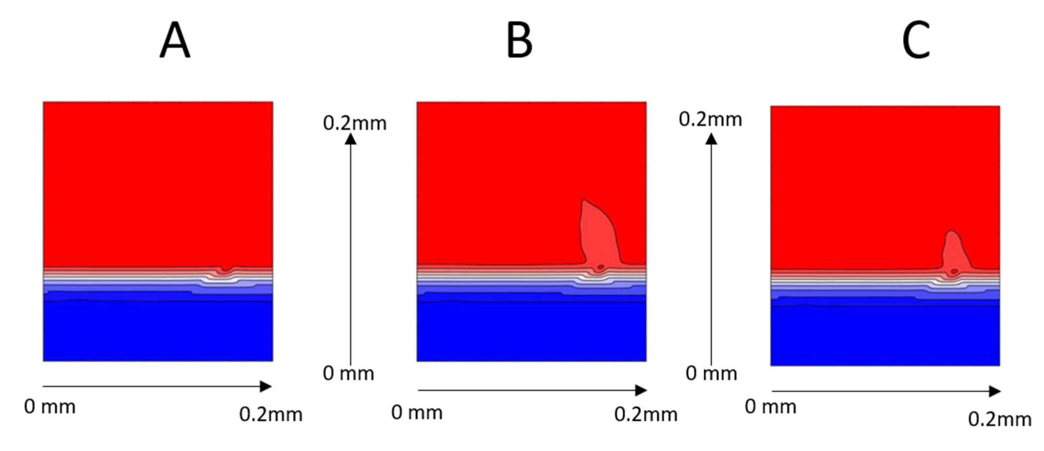
Figure 5.
Two-dimensional slides of time-averaged DNS results of statistically planar premixed flames in cases (A–C). The colour range for filtering of flame fronts is from 1000 K (blue) to 3000 K (red).
Figure 5.
Two-dimensional slides of time-averaged DNS results of statistically planar premixed flames in cases (A–C). The colour range for filtering of flame fronts is from 1000 K (blue) to 3000 K (red).

Figure 6.
(Left): Adapted regime diagram with coloured visualisation of normalised mesh sizes based on Equation (21). The considered is the characteristic value from within the flame according to the definition in Section 3.3. Different works with different are noted. (Right): Flame front resolutions and domain to Eddy size ratios in different works.

Figure 7.
Laminar flame parameters for methane–oxygen combustion at K.

Figure 8.
Pr development throughout the flame front. T is normalised with . is determined according to Equation (12). is determined according to Equation (9). “Cut-out” indicates the magnified area. Conditions: Stochiometric O2/CH4 mixture at 20 bar and initial temperature of 350 K. The upper range of the blue line of , where it converges to a stable value, is cut out due to its irrelevance to the current problem.

Figure 9.
Modified regime diagram for premixed Flames with non-changing isoline for . Simulations of different operating points are plotted. The arrows indicate how the relative positions of several example cases change due to the modification of the x-axis.
Figure 9.
Modified regime diagram for premixed Flames with non-changing isoline for . Simulations of different operating points are plotted. The arrows indicate how the relative positions of several example cases change due to the modification of the x-axis.


Table 1.
Characteristics of the simulated cases.
| Case | A | B | C |
|---|---|---|---|
| 2.2 | 4.59 | 7.55 | |
| 40.6 | 31 | 30.7 | |
| 1.5 | 0.81 | 0.56 | |
| 0.74 | 1.37 | 1.98 | |
| 3.072 | 3.072 | 3.072 | |
| 5.46 | 5.46 | 5.46 | |
| 1.11 | 1.11 | 1.11 | |
| 11.8 | 11.8 | 11.8 | |
| 80.5 | 128 | 209 | |
| 0.87 | 1.37 | 5.48 | |
| 10.38 | 3.8 | 2.3 | |
| 8 | 8 | 8 | |
| 7 | 7 | 7 | |
| 4 | 4 | 4 |
Table 2.
Definitions of Pr in Figure 8.
Table 2.
Definitions of Pr in Figure 8.
| Point | Definition | Determination Method | Pr | |
|---|---|---|---|---|
variable constant | from reactants | 0.066 | 1.11 | |
| Favre-averaged ν | 0.817 | 13.7 | ||
| Averaged ν | 1.564 | 26.2 | ||
| 2.014 | 33.8 | |||
Whole Pr term as a local variable | from reactants | 0.717 | 1.11 | |
| Position of autoignition temperature | 0.704 | 4.45 | ||
| Favre averaged Pr | 0.691 | 22.1 | ||
| Averaged Pr | 0.676 | 29.1 | ||
| 0.675 | 29.9 | |||
| Intersection of both definitions | 0.706 | 11.8 |
Publisher’s Note: MDPI stays neutral with regard to jurisdictional claims in published maps and institutional affiliations. |
© 2022 by the authors. Licensee MDPI, Basel, Switzerland. This article is an open access article distributed under the terms and conditions of the Creative Commons Attribution (CC BY) license (https://creativecommons.org/licenses/by/4.0/).
Share and Cite
MDPI and ACS Style
Sternin, A.; Martinez, D.; Sternin, D.; Haidn, O.; Tajmar, M. Characterisation and Design of Direct Numerical Simulations of Turbulent Statistically Planar Flames. Aerospace 2022, 9, 530. https://doi.org/10.3390/aerospace9100530
AMA Style
Sternin A, Martinez D, Sternin D, Haidn O, Tajmar M. Characterisation and Design of Direct Numerical Simulations of Turbulent Statistically Planar Flames. Aerospace. 2022; 9(10):530. https://doi.org/10.3390/aerospace9100530
Chicago/Turabian StyleSternin, Andrej, Daniel Martinez, Daniel Sternin, Oskar Haidn, and Martin Tajmar. 2022. "Characterisation and Design of Direct Numerical Simulations of Turbulent Statistically Planar Flames" Aerospace 9, no. 10: 530. https://doi.org/10.3390/aerospace9100530
Note that from the first issue of 2016, this journal uses article numbers instead of page numbers. See further details here.