
Attitude Stabilization of a Satellite Having Only Electromagnetic Actuation Using Oscillating Controls


1
Department of Electronic Systems, Automation and Control, Aalborg University, Fredrik Bajers Vej 7 C, 9220 Aalborg, Denmark
2
Max Planck Institute for Dynamics of Complex Technical Systems, Otto von Guericke University Magdeburg, 39106 Magdeburg, Germany
3
Institute of Applied Mathematics and Mechanics, National Academy of Sciences of Ukraine, G. Batyuka 19, 84116 Sloviansk, Ukraine
*
Author to whom correspondence should be addressed.
Aerospace 2022, 9(8), 444; https://doi.org/10.3390/aerospace9080444
Submission received: 18 April 2022
/
Revised: 5 August 2022
/
Accepted: 9 August 2022
/
Published: 13 August 2022
(This article belongs to the Special Issue Spacecraft Attitude Control Using Magnetic Actuators)
Abstract
:We consider the problem of attitude stabilization for a low Earth orbit satellite having only electromagnetic actuation. Such a satellite is not fully actuated, as the control torque is the cross-product of magnetic moment due to magnetorquers and the geomagnetic field. The aim of this work is to study whether oscillating controls can be designed such that a satellite actuated via magnetorquers alone can achieve full three-axis control irrespective of the position of the satellite. To this end, we propose considering oscillating feedback controls which generate the motion of the closed-loop system in the direction of appropriate Lie brackets. Simulation studies show that the proposed control scheme is able to stabilize the considered system.
1. Introduction
In this work, we consider the attitude stabilization problem for a low Earth orbit satellite. The attitude of a satellite is its orientation in the orbital coordinate system and is defined by an attitude matrix which is parameterized by unit quaternions (see [1] for a survey on the application of quaternions for the orientation of rigid bodies). Attitude stabilization can be achieved by applying external torque on the satellite, which is described via Euler’s equations [2]. Besides the torque due to the magnetorquers, the control torque can be provided via gas jets and reaction wheels. The books [3,4] provide an overview of control techniques for the attitude stabilization problem. In this work, we consider a satellite having only electromagnetic actuation. Since such a satellite is actuated via a renewable energy source, it has a longer usable life compared to other actuation techniques. However, it suffers from controllability limitations as the control torque is provided by the cross-product of the geomagnetic field and magnetic moment generated by the satellite’s magnetic coils. Specifically, the control torque is constrained to lie in the plane orthogonal to the geomagnetic field, and therefore, full three-axis control is not possible at all attitudes. However, as the satellite’s position is varying on its orbital plane, correspondingly, the geomagnetic field also varies, and this results in the overall dynamical system being periodic with a frequency depending on the orbital rate of the satellite. Such a nonlinear periodic system is controllable [5,6]. There have been many works on satellites actuated via magnetorquers alone. In [7], full three-axis control is obtained by dividing the dynamics into two loops (inspired by the backstepping method from [8]). A sliding mode controller is used for tracking in the inner loop, and the outer loop is used for stabilization. In [9], the performance of three different control schemes (Detumbling, Linear-Quadratic-Regulator (LQR) and Proportional-Derivative (PD) controls) are compared. The survey paper [10] surveys applications of model-predictive control for such satellites, and the survey paper [11] along with the references therein provide an overview of the present state-of-art in attitude stabilization for satellites having only electromagnetic actuation. To the best of the authors’ knowledge, the current state-of-art in attitude stabilization of satellite relies on the periodic nature of the geomagnetic field to ensure stability given the controllability restriction of a satellite actuated via magnetorquers alone.
In this work, we study whether oscillating controls can be designed such that a satellite actuated via magnetorquers alone can achieve full three-axis control irrespective of the position of the satellite and almost time-invariant geomagnetic field. In order to overcome the aforementioned control theoretic challenges, we consider here oscillating controls in addition to the PD controls discussed in [6]. These oscillating controls are motivated from the literature on the control of underactuated systems [12] and are based on the fact that the considered class of systems admits a time-varying stabilizing feedback law, provided that the local controllability and regularity assumptions as mentioned in [13] are satisfied. The oscillating controls are sinusoidal in nature and generate motion along the direction of Lie brackets of vector fields of the considered dynamical system. The book [14] provides a review on properties of Lie brackets. A generalized design procedure of stabilizing oscillating controls for driftless control-affine systems is presented in [15], and the inclusion of drift is discussed in [16]. The primary aim of this work is to investigate whether oscillating controls can provide sufficient time variation such that full three-axis control can be achieved on a satellite actuated via magnetorquers alone irrespective of the position of the satellite. The control methodology developed subsequently archives full three-axis control in the case of a slowly varying magnetic field. Further work is required to address practical considerations such as magnetorquer saturation, residual magnetic moment and disturbances such as areodynamic drag.
The rest of the paper is organized as follows. In Section 2, we review the mathematical model of the satellite. We rewrite the aforementioned mathematical model in the control-affine form and pose the motivating question in Section 3. Thereafter, we design Lie bracket-based controls in Section 4. Simulation studies are presented in Section 5, and lastly, Section 6 provides the conclusions of this work.
2. Mathematical Model
We begin by stating general coordinate systems (CS) and notations for the satellite.
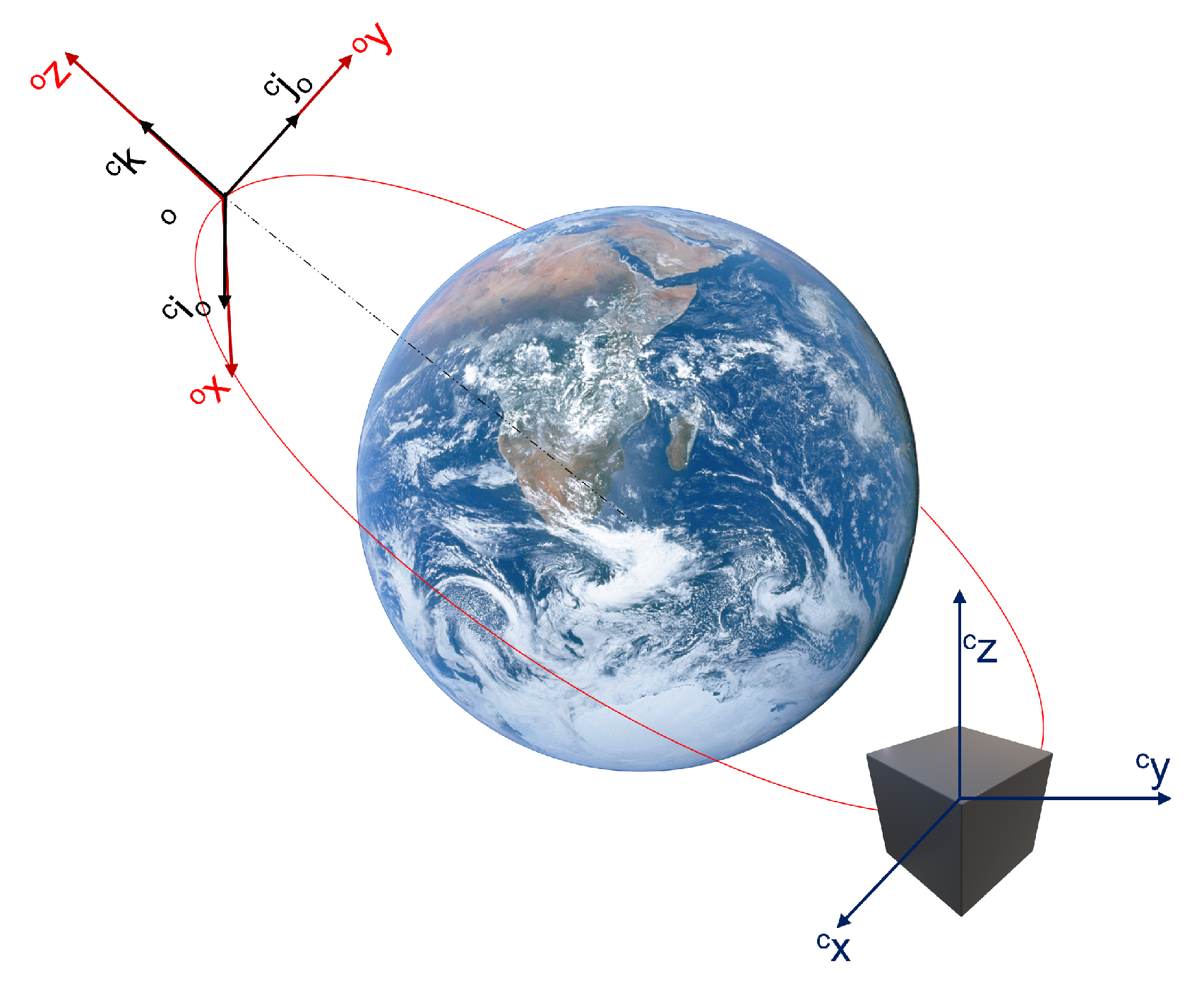
A pictorial representation of the CS is described in Figure 1 with description of CS given in Table 1. In the sequel, the superscripts represent the vector in parentheses expressed in BCS, OCS and WCS, respectively, and the subscripts represent the angular velocity in BCS with respect to WCS and the angular velocity in BCS with respect to OCS.
The equations of motion of a rotating satellite with electromagnetic actuation are governed by kinematics and rigid body dynamics. The kinematics represent the attitude of the rotating satellite and are described via the following equation:
where q (consisting of three components , , ) denotes the vector part of the attitude quaternion, which represents the rotation of the satellite in the BCS with respect to OCS, and is the scalar component of the attitude quaternion. The scalar part is not unique, but is constrained as follows:
In this work, we consider only the kinematics of the vector part of the attitude quaternion in (1) and enforce quaternion constraint (2) by considering the space of q as a ball in with . The rotation of the satellite in OCS with respect to the BCS is described using the attitude matrix, which is defined as follows:
where and are the unit vectors representing the and z axes of the OCS projected on the BCS. The components and of are parameterized by the attitude quaternion q and are defined as follows:
The dynamics of the satellite represents the time evolution of the angular velocity in OCS. The angular velocity in OCS can be obtained from the angular velocity defined in WCS by
where is the orbital rate which will be considered a constant in this work, as the eccentricity of the considered satellite’s orbit is negligible. The Euler equation of the satellite in WCS can be stated as follows:
where is the control torque, is the torque due to the gravitational gradient, and the remaining terms represent the classical Euler equations as given in [2]. In this work, we have not considered disturbance torque due to the aerodynamic drag and the residual magnetic field as our aim is to study whether oscillating controls can be designed such that a satellite actuated via magnetorquers alone can achieve full three-axis control irrespective of the position of the satellite. Therefore, for the sake of simplicity, we neglect the disturbance torques. Substituting (5) in (6) gives us
Simplifying (7) gives us
The control torque in (8) is generated via electromagnetic actuation. Such actuators are known as magnetorquers, and they generate control torque via interaction between magnetic coils stored in the satellites body and the geomagnetic field due to Earth. Mathematically, is defined as follows:
where represents the magnetic moment generated by the satellite, and represents the geomagnetic field. The satellite’s magnetic moment is generated via magnetic coils housed inside the satellite body as follows:
where is the number of windings of the coil, is the current in the coil, and is the area of the coil. The electromagnetic coils are placed perpendicular to the x, y and z axis, and thus, m is a vector with components and . For the rest of the paper, m represents the control signal. For the purpose of simulation studies in this work, the geomagnetic field vector is approximated via the dipole model given in [3]. Let , , represent the empirical Gaussian coefficients of the standard model of Earth’s geomagnetic field. The dipole model in OCS can then be stated as follows:
where a is the radius of Earth, r is the geocentric distance of the satellite, is the co-elevation of the dipole model, is the east longitude of the dipole model, is the right ascension of the dipole model, is the true anomaly measured from the ascending node and is used to calculate the total dipole strength. Furthermore, and are calculated as follows:
The cosine and sine components of the dipole model have been approximated by a harmonic oscillator. The harmonic oscillator is a 2nd order differential equation, which is described as follows:
where is frequency of the oscillations, and are the oscillating states representing the cosine and sine components of the dipole model. The solution of (13) approximates the cosine and sine components due to . Additional harmonic oscillators can be added for more accurate approximations at the cost of adding extra states to the system. The gravity gradient torque is also considered in the model, and it can be stated using the attitude matrix (3) third row k as done in [3], as follows:
In the sequel, without subscripts or superscripts represents .
3. Problem Statement
We rewrite system (1)–(8) in the control-affine form as follows:
where , X is a neighborhood of in such that X does not contain any nontrivial equilibrium of (15) with ,
For the control design, we consider the following Lyapunov function candidate
where is a scalar constant. Then, the directional derivative of along the vector field is
and the time derivative of V along the trajectories of (15) can be written as
As the scalar triple product is unchanged under a circular shift of its operands, we have
with
Recall that a positive definite function of class is said to be a control Lyapunov function (CLF) for a system of the form , , [17], if, for any , there exists a vector such that . Similarly, we call a weak CLF if [18], for any , there is a such that . By Artstein’s theorem [19], the existence of a CLF is equivalent to the existence of a stabilizing feedback law of the form , for nonlinear control-affine systems. We will see that the design methodology based on Artstein’s theorem (and its extension with a weak CLF [18]) is not directly applicable in our case. Indeed, as one can easily deduce from the expression (19), a necessary and sufficient condition for the function to be a weak CLF for (15) is that
Condition (20) can be equivalently written in the following form: “for each , either or ( and )”.
We show that condition (20) is violated because the geomagnetic field . Indeed, the condition for is equivalent to
Then, by substituting the above into , we get
which takes positive values under a suitable choice of whenever . Thus, the only possibility to satisfy the condition (20) for any x and at the points is to have . However, we see that the latter property holds only for due to the structure of in (3). Hence, the candidate Lyapunov function is not a weak CLF for system (15).
To overcome the above-mentioned constraint for pure Lyapunov-based control design, we will propose a “hybrid” control strategy based on a combination of state feedback controllers with -periodic oscillating input signals, where is treated as a small parameter. Such a construction is inspired by the fact that takes positive values at some with any admissible choice of controls u. Thus, the objective of our oscillating control component is to ensure the decreasing of on time intervals of length when the time derivative is not negative.
To be precise, we introduce a parameter and split the whole state space into the union of two disjoint sets ,
where
In the sequel, we will consider the following two cases:
- ;
- .
Consider first the case . This implies that . We can define the following state feedback law (pre-compensator) aiming to stabilize the trivial solution of system (15)
where is a design parameter. Note that formula (24) also contains the design parameter originating from (16). Then, the time derivative along the trajectories of the closed-loop system (15), (24) takes the form
The following Lemma proves the existence of a globally stabilizing control law for the case when . This should be seen as an alternative to the locally stabilizing PD controls discussed in the literature [6,11].
Lemma 1.
Proof.
We now consider the case and we pose the following question: is it possible to ensure
for all by applying -periodic oscillating controllers for some ? We show in the following section that this is indeed the case if we consider oscillating controls with sine and cosine terms.
4. Lie Bracket-Based Control in
In this section, we construct -periodic controllers that ensure the decreasing of along the trajectories in . The solutions of system (15) corresponding to the initial data and admissible controls can be represented by the Chen–Fliess expansion:
where denotes the directional derivative of along the vector field , and stands for higher-order terms. The Chen–Fliess series are reviewed in [20]. The overall control scheme comprises a time-invariant feedback component with an oscillating component and is similar to the generalized periodic controls presented in [15,16]. Let be a small parameter which controls the oscillating frequency; then, we define the control functions as follows:
where , , , , , are treated as real parameters, and , and are nonzero integers such that their magnitudes are mutually distinct numbers. We substitute controls (29) into the Chen–Fliess expansion (28) and compute the Taylor series expansion of for small :
where represents the Lie brackets of vector fields and . The idea behind our control scheme is to construct the above , , , , , , depending on the current system state, such that (30) guarantees
and thereby ensure along nontrivial trajectories of (15).
If is chosen in such a way that its component is not parallel to , then because of (21). Thus, by putting in (29), we see that the condition (31) is satisfied with the control parameters
at , where is given by (24) provided that is large enough.
Consider now the case and , where indicates that the magnetic field in OCS is almost time-invariant (for example, if the satellite is following an equatorial orbit). This implies , so that , and the property (31) can be ensured by defining
at , provided that the gain is large enough and at least one of the Lie brackets in (33) does not vanish at . To formalize this scheme, we introduce the following assumption.
Assumption 1.
The vector fields satisfy the following nonsingularity condition for each and :
where we treat B as a parameter in , , , , , and .
From the geometric viewpoint, condition (34) means that the gradient of is not perpendicular to the linear span
for each in and each admissible value of the geomagnetic field. Then, it is possible to ensure the decreasing of along the trajectories of (15) in whenever one can implement the motion along the directions ,, and .
5. Simulation Results
In this section, we present simulation results on the closed-loop system (15) using controls (29). The geomagnetic field was simulated using (11) with (13). The empirical Gaussian coefficients used in the simulations are obtained from the IGRF model. The inertia (in ) tensor of the satellite is given as
In all the simulation results, the frequency parameter is , and the controller parameters are shown in Table 2. The form of control law (24) makes it undesirable for practical implementation (as as ). We have therefore implemented a locally stable PD controller based on Chapter 4 in [6] when the satellite trajectory is . The gain parameters for the PD controller were found in the following way. We considered the case when (i.e., control scheme (33) is not active) and began by tuning the derivative gains until we stabilized the angular velocities. Thereafter, we tuned the proportional gains such that the kinematics were stabilized.
The altitude of the orbit is 800 km. We ran the simulations with a geomagnetic field that is almost time-invariant as can be seen in Figure 2 and initialized (15) in .
In Figure 3, we can observe the stability of (15) if the satellite was operating in the situation of an almost time-invariant geomagnetic field and (15) were initialized in . During the transient phase (i.e., up to the 4th orbit), we observe high-frequency oscillations up to the 2nd orbit and thereafter, the frequency of oscillations is markedly decreased between the 2nd and the 4th orbit, culminating in stabilization around the 4th orbit. Note that, at the equilibrium point, is equal to , while , and are 0, and this is due to the quaternion constraint (2).
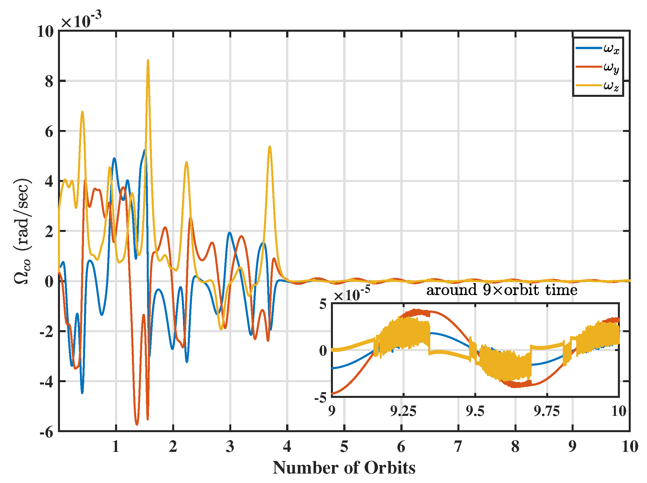
In Figure 4, we observe the angular velocity corresponding to Figure 3. The initial angular velocity considered in the simulation can be attained by a damping law (referred to as B-dot law in literature [11]), and attitude maneuvering should be started once the initial velocity is reasonably low. It should be noted that the equilibrium point, as in (19) (since ). Consequently, (33) is activated at this point, and therefore, we observe high frequency oscillations at the steady state in Figure 4.
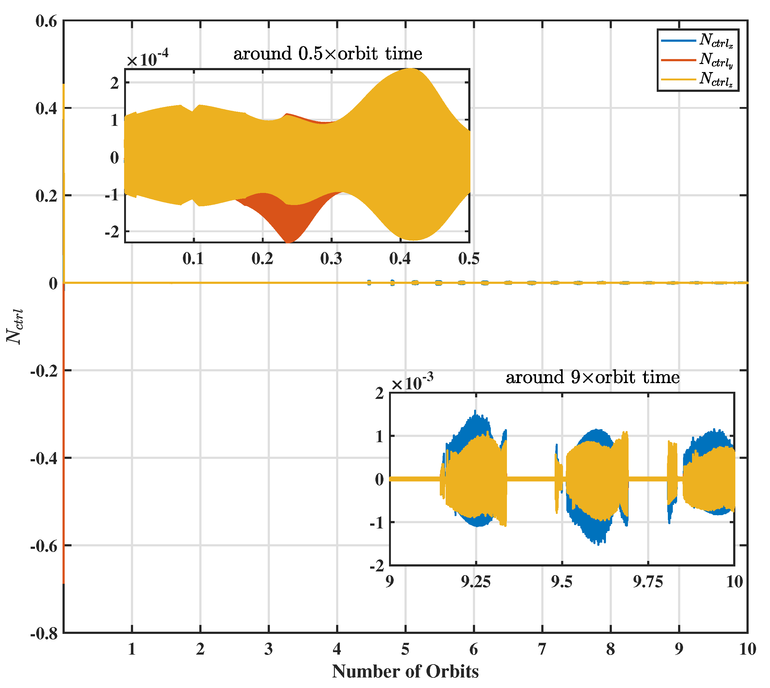
The high-frequency oscillations in the zoomed-in part of Figure 4 are due to the oscillating controls. Figure 5 represents the control torque, and the relatively high torque values in the beginning limit the practical application of this work. In future work, we plan to study these controls with saturation limits included in (29) (imposing saturation limits in an ad hoc manner results in an unstable behavior) to simulate the real-world situation more closely.
6. Conclusions and Future Work
In this work, we have proposed an oscillating control scheme for the attitude stabilization of satellite actuated via magnetorquers alone. Simulation results show that the proposed oscillating controls scheme manages to stabilize the attitude and angular velocity in the case of a slowly varying magnetic field. However, the control torque was quite high, and therefore, this technique still needs to be refined. Also, this work does not yet address disturbances due to aerodynamic drag and residual magnetic field. Furthermore, a formal proof is still lacking due to technical challenges in estimating the Chen–Fliess terms of different orders with respect to components of the state vector, particularly in the case of a time-varying geomagnetic field.
Possible future work could be to either find a better candidate Lyapunov function or to use another technique such as combinations of Lyapunov and density functions to prove the stability of the closed-loop system. Another challenging future work is to simulate whether the magnetically actuated satellite with the proposed control scheme can follow an orbit in the geomagnetic equatorial plane. Consequently, for all time, and the Lie bracket-based controller (33) will be active always. Unfortunately, due to the limitations of the conventional Ordinary Differential Equations (ODE) solver, we could not simulate this scenario satisfactorily. Specifically, due to the oscillating nature of (29), the ODE solver could not maintain the error tolerances without reducing the step-size to a very low value. Therefore, further investigation is required in this direction, as the small step-size may lead to problems both in the pulse-width modulation implementation and in the residual magnetization of magnetorquers. To summarize, we can conclude that oscillating controls represent a potential research direction in addressing the challenging problem of active three-axis control using magnetorquers only.
Author Contributions
Conceptualization, A.Z., R.W. and R.M.; methodology, A.Z.; software, R.M. and A.Z.; validation, R.M. and R.W.; formal analysis, R.M., R.W. and A.Z.; investigation, R.M.; data curation, R.M.; writing—original draft preparation, R.M.; writing—review and editing, R.W. and A.Z.; visualization, R.M.; supervision, R.W. and A.Z.; project administration, R.M.; funding acquisition, A.Z. and R.W. All authors have read and agreed to the published version of the manuscript.
Funding
The first and the second author were supported by the Poul Due Jensen Foundation (Grundfos Foundation) under the project SWIfT, and the third author was supported by the German Research Foundation (DFG) under Grant ZU 359/2-1.
Data Availability Statement
Not Applicable.
Conflicts of Interest
The authors declare no conflict of interest.
References
- Stuelpnagel, J. On the parametrization of the three-dimensional rotation group. SIAM Rev. 1964, 6, 422–430. [Google Scholar] [CrossRef]
- Goldstein, H. Classical Mechanics; Pearson Education India: Noida, India, 2011. [Google Scholar]
- Wertz, J.R. Spacecraft Attitude Determination and Control; Springer Science & Business Media: Berlin/Heidelberg, Germany, 1978; Volume 73. [Google Scholar]
- Markley, F.L.; Crassidis, J.L. Fundamentals of Spacecraft Attitude Determination and Control; Springer: Berlin/Heidelberg, Germany, 2014; Volume 33. [Google Scholar]
- Bhat, S.P.; Dham, A.S. Controllability of spacecraft attitude under magnetic actuation. In Proceedings of the 42nd IEEE International Conference on Decision and Control (IEEE Cat. No. 03CH37475), Maui, HI, USA, 9–12 December 2003; Volume 3, pp. 2383–2388. [Google Scholar]
- Wisniewski, R. Satellite Attitude Control Using Only Electromagnetic Actuation. Ph.D. Thesis, Department of Control Engineering, Aalborg University, Aalborg, Denmark, 1996. [Google Scholar]
- Wang, P.; Shtessel, Y.B. Satellite attitude control using only magnetorquers. In Proceedings of the 1998 IEEE American Control Conference. ACC (IEEE Cat. No. 98CH36207), Morgantown, WV, USA, 10 March 1998; Volume 1, pp. 222–226. [Google Scholar]
- Krstic, M.; Kokotovic, P.V.; Kanellakopoulos, I. Nonlinear and Adaptive Control Design; John Wiley & Sons: Hoboken, NJ, USA, 1995. [Google Scholar]
- Torczynski, D.; Amini, R.; Massioni, P. Magnetorquer based attitude control for a nanosatellite testplatform. In Proceedings of the AIAA Infotech@ Aerospace, Atlanta, GA, USA, 20–22 April 2010; p. 3511. [Google Scholar]
- Eren, U.; Prach, A.; Koçer, B.B.; Raković, S.V.; Kayacan, E.; Açıkmeşe, B. Model predictive control in aerospace systems: Current state and opportunities. J. Guid. Control. Dyn. 2017, 40, 1541–1566. [Google Scholar] [CrossRef]
- Ovchinnikov, M.Y.; Roldugin, D. A survey on active magnetic attitude control algorithms for small satellites. Prog. Aerosp. Sci. 2019, 109, 100546. [Google Scholar] [CrossRef]
- Murray, R.; Sastry, S. Nonholonomic motion planning: Steering using sinusoids. IEEE Trans. Autom. Control. 1993, 38, 700–716. [Google Scholar] [CrossRef]
- Coron, J.M. Control and Nonlinearity; Number 136; American Mathematical Society: Providence, RI, USA, 2007. [Google Scholar]
- Isidori, A. Nonlinear Control Systems; Springer: Berlin/Heidelberg, Germany, 1995; Volume 3. [Google Scholar]
- Zuyev, A. Exponential stabilization of nonholonomic systems by means of oscillating controls. SIAM J. Control. Optim. 2016, 54, 1678–1696. [Google Scholar] [CrossRef]
- Zuyev, A.; Grushkovskaya, V. On stabilization of nonlinear systems with drift by time-varying feedback laws. In Proceedings of the 12th IEEE International Workshop on Robot Motion and Control (RoMoCo), Poznan, Poland, 8–10 July 2019; pp. 9–14. [Google Scholar]
- Sontag, E. A ‘universal’ construction of Artstein’s theorem on nonlinear stabilization. Syst. Control Lett. 1989, 13, 117–123. [Google Scholar] [CrossRef]
- Zuyev, A. Application of control Lyapunov functions technique for partial stabilization. In Proceedings of the 2001 IEEE International Conference on Control Applications CCA’01, Mexico City, Mexico, 7 September 2001; pp. 509–513. [Google Scholar]
- Artstein, Z. Stabilization with relaxed controls. Nonlinear Anal. Theory Methods Appl. 1983, 7, 1163–1173. [Google Scholar] [CrossRef]
- Lamnabhi-Lagarrigue, F. Volterra and Fliess Series Expansions for Nonlinear Systems. In The Control Systems Handbook; CRC Press: Boca Raton, FL, USA, 2018; pp. 957–974. [Google Scholar]
Figure 1.
The coordinate system can be visualized in this figure. BCS is centered on the spacecraft’s body (represented by the blue CS centered on the black cube’s center of mass). OCS is fixed on the orbit (represented by the red CS fixed on the red orbit), and the unit vectors and are aligned with the OCS (represented by the black CS). The unit vector is pointing in the direction of orbital angular velocity vector (therefore, orthogonal to orbital plane), and the unit vector is pointing away from the center of the earth (shown by dotted line).

Figure 2.
The magnetic field considered in the simulation studies is almost time-invariant. , and are the components of the dipole model in OCS (11) in the case when the satellite is following an circular equatorial orbit (see Equation (H-30) in [3]).

Figure 3.
Quaternions achieve stability (up to an error represented in terms of Euler angles) with the initial quaternion despite an almost time-invariant magnetic field.
Figure 3.
Quaternions achieve stability (up to an error represented in terms of Euler angles) with the initial quaternion despite an almost time-invariant magnetic field.

Figure 4.
Angular velocities achieve stability (up to an error bound) with initial , , , despite an almost time-invariant magnetic field. The oscillations seen in the zoomed-in part around the 9th orbit are due to the oscillating controls.
Figure 4.
Angular velocities achieve stability (up to an error bound) with initial , , , despite an almost time-invariant magnetic field. The oscillations seen in the zoomed-in part around the 9th orbit are due to the oscillating controls.

Figure 5.
The control torque in N-m corresponding to Figure 3 and Figure 4. The control torque has a high magnitude in the beginning, and this limits the practical application to an extent. The chattering seen in the zoomed-in part around 9th orbit is due to the oscillating controls.

Figure 6.
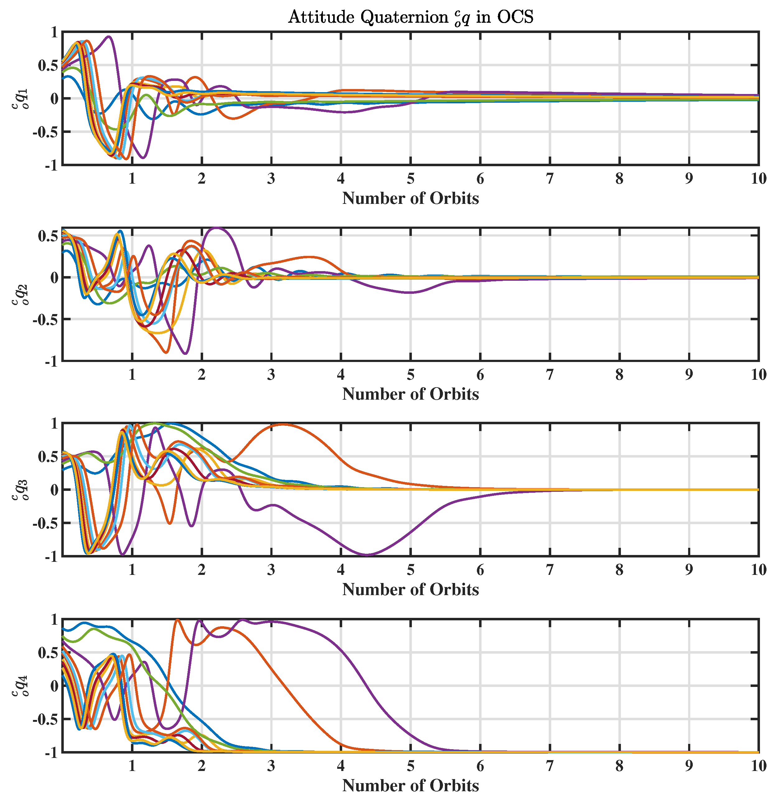
Quaternions converging to the local equilibrium point after starting from random initial quaternions (in a local neighbourhood). Subplots 1–4 represent quaternions –, respectively.
Figure 6.
Quaternions converging to the local equilibrium point after starting from random initial quaternions (in a local neighbourhood). Subplots 1–4 represent quaternions –, respectively.

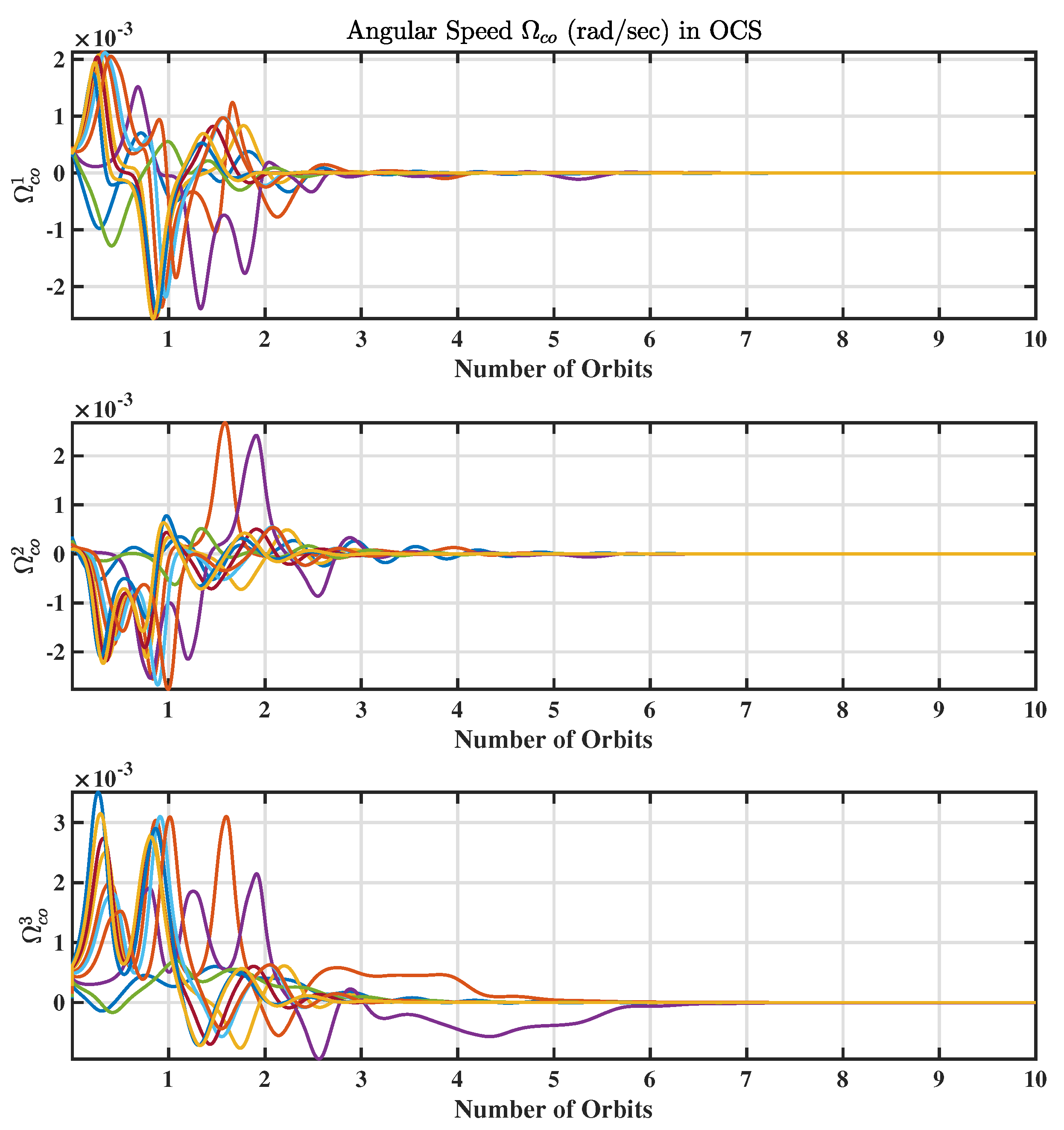
Figure 7.
Angular velocities converging to the local equilibrium point after starting from random initial quaternions (in a local neighbourhood). Subplots 1–3 represent angular velocities –, respectively.
Figure 7.
Angular velocities converging to the local equilibrium point after starting from random initial quaternions (in a local neighbourhood). Subplots 1–3 represent angular velocities –, respectively.


Table 1.
Coordinate system.
| Acronym | Name | Description |
|---|---|---|
| BCS | Body (or Control) Coordinate System | CS built on principal axes of inertia of the satellite |
| OCS | Orbital Coordinate System | Reference CS fixed in the orbit |
| WCS | World Coordinate System | Inertial right orthogonal CS |
Table 2.
Controller parameters used in simulations.
| Value | 0.0375 | 0.0375 | 0.1875 | 55 | 60 | 35 | 1 | 2 | 3 |
Publisher’s Note: MDPI stays neutral with regard to jurisdictional claims in published maps and institutional affiliations. |
© 2022 by the authors. Licensee MDPI, Basel, Switzerland. This article is an open access article distributed under the terms and conditions of the Creative Commons Attribution (CC BY) license (https://creativecommons.org/licenses/by/4.0/).
Share and Cite
MDPI and ACS Style
Misra, R.; Wisniewski, R.; Zuyev, A. Attitude Stabilization of a Satellite Having Only Electromagnetic Actuation Using Oscillating Controls. Aerospace 2022, 9, 444. https://doi.org/10.3390/aerospace9080444
AMA Style
Misra R, Wisniewski R, Zuyev A. Attitude Stabilization of a Satellite Having Only Electromagnetic Actuation Using Oscillating Controls. Aerospace. 2022; 9(8):444. https://doi.org/10.3390/aerospace9080444
Chicago/Turabian StyleMisra, Rahul, Rafał Wisniewski, and Alexander Zuyev. 2022. "Attitude Stabilization of a Satellite Having Only Electromagnetic Actuation Using Oscillating Controls" Aerospace 9, no. 8: 444. https://doi.org/10.3390/aerospace9080444
Note that from the first issue of 2016, this journal uses article numbers instead of page numbers. See further details here.