
Fluid-Structure Interaction Modelling of a Soft Pneumatic Actuator


1
Workgroup on System Technologies and Engineering Design Methodology, Hamburg University of Technology TUHH, 21073 Hamburg, Germany
2
Fraunhofer Research Institution for Additive Manufacturing Technologies IAPT, 21029 Hamburg, Germany
*
Author to whom correspondence should be addressed.
Actuators 2021, 10(7), 163; https://doi.org/10.3390/act10070163
Submission received: 1 June 2021
/
Revised: 8 July 2021
/
Accepted: 11 July 2021
/
Published: 15 July 2021
(This article belongs to the Section Actuators for Robotics)
Abstract
:This paper presents a fully coupled fluid-structure interaction (FSI) simulation model of a soft pneumatic actuator (SPA). Previous research on modelling and simulation of SPAs mostly involves finite element modelling (FEM), in which the fluid pressure is considered as pressure load uniformly acting on the internal walls of the actuator. However, FEM modelling does not capture the physics of the fluid flow inside an SPA. An accurate modelling of the physical behaviour of an SPA requires a two-way FSI analysis that captures and transfers information from fluid to solid and vice versa. Furthermore, the investigation of the fluid flow inside the flow channels and chambers of the actuator are vital for an understanding of the fluid energy distribution and the prediction of the actuator performance. The FSI modelling is implemented on a typical SPA and the flow behaviour inside the actuator is presented. Moreover, the bending behaviour of the SPA from the FSI simulation results is compared with a corresponding FEM simulation.
1. Introduction
Soft robots are made of soft and compliant materials, providing multiple degrees of freedom, and, unlike traditional robots that are made of rigid bodies, soft robots provide a safe environment for human-robot interaction [1,2]. They are predominantly inspired from natural systems and are operated at relatively low cost. Soft robots are capable of performing diverse actions such as grasping and manipulation, locomotion, squeezing, climbing, jumping, and growing [1]. They can be used for many applications in various fields. For example, in the medical field, for designing soft surgical instruments [3], soft rehabilitation devices such as single fingers [4,5], hands [6], wrists [7], and elbows [8,9], as well as for the colonoscopy process [10]. Besides the medical field, their applications include exploration and rescue operations [11,12], gripping and manipulation of fragile and/or unknown objects [13], human-machine interfaces [14], and unmanned underwater vehicles [15].
Soft actuators [16,17,18] are among the most important structural and functional elements of soft robots. Their proper function has a significant impact on the overall performance of soft robotic systems. Soft actuators are driven in various ways, such as pneumatically, hydraulically, electrically, or chemically [19]. Here, we focus on soft pneumatic actuators (SPAs), as they are inexpensive, have a high power-to-weight ratio, and provide safe human-robot interaction. There are different types of SPAs based on their function, such as bending, extension, contraction, and twisting [20]. The different functions can be realised by a different arrangement of inextensible elements. The multiple degrees of freedom offered by soft robots enables the development of novel soft robotics systems with enhanced dexterity through different combinations of actuators, chambers, or other parts [21,22,23,24].
Bending SPAs are widely used in soft robotics for medical applications [25], such as in prosthetic and rehabilitation devices and for grasping and manipulation [13]. The pneumatic networks (PneuNets) concept, which was proposed by Mosadegh et al. [26], is mostly favoured in the context of bending SPAs. The performance of PneuNets actuators strongly depends on the design parameters of the air channels and the internal chambers. Therefore, the development of a proper modelling and simulation technique of PneuNets actuators is essential for the design, development, and optimization of soft robots. Usually, the finite element method (FEM) is used to predict the behaviour of actuators and to optimize their design. In this case, the applied pneumatic pressure is considered to be the pressure load acting uniformly on the walls of the inner chambers. This pressure, however, is applied instantly to all actuator chambers, which, in reality, is not the case. The fluid energy distribution inside of soft robots influences their performance from a small to large extent depending on its design and the rate of pressurization, among other factors. Mosadegh et al. [26] demonstrated experimentally that, for the single actuator design, at least two different types of motion can be obtained by changing the rate of pressurization. This clearly indicates that the rate of pressurization is one of the important factors that influences the fluid pressure distribution, and, as a result, the actuator’s performance differs. For this reason, the physics of the fluid flow inside the actuators must be considered for a proper actuator design. These can be captured by considering the fluid-structure interaction (FSI) of the fluid and the deformable bodies.
In addition to FEM, analytical models have also been developed for soft actuators. For example, Polygerinos et al. [27] proposed a quasi-static analytical model based on Newton’s method for the behaviour of a fibre-reinforced soft actuator to obtain a relationship between input pressure, bending angle, and output force. Connolly et al. [28] used a kinematic trajectory as an input for developing a nonlinear elasticity-based analytical model for fibre-reinforced soft actuators. The authors mentioned that, although their analytical model is less computationally intense than the FEM model, the FEM model is more accurate. In addition, the above models assumed uniform bending curvature and neglected the air pressure dynamics. Yang et al. [29] presented a kinematic-static coupling model based on screw rod theory and the principle of minimum potential energy on an eccentric soft bending fibre-reinforced actuator. For pneumatic bending actuators, Gu et al. [30] proposed an analytical model based on minimum potential energy method and continuum rod theory. However, all the models assumed uniform pressure distribution on the inner cavities of the actuators. Regarding flow dynamics, Breitman et al. [31] proposed an analytical model using long-wave approximation for compressible viscous flow in elastic media and illustrated it on a miniaturized pneumatic soft robot. The model provided insights on actuation dynamics, especially the pressure distribution inside the flow chambers. Overall, analytical models quickly provide insights to the actuator’s behaviour (for a particular geometry) upon pressurization, and they are relatively inexpensive to solve. However, the proper assumptions made in analytical modelling are challenging and they do not solve for the parameters’ pressure, velocity, stress, strain, displacement, contact forces, etc., altogether, as illustrated in the above references. Simulation models provide more realistic descriptions of the actuator’s behaviour, and the solutions can be readily visualized [27]. Furthermore, a fully coupled FSI model can solve the above-mentioned parameters altogether, though at the expense of computational cost. Mostly, FSI or, in general, multiphysics problems are very complex to solve analytically, which is why they are predominantly solved using numerical simulations or experiments [32].
Very few FSI analyses have been conducted in soft robotics applications. Moon et al. [33] proposed an FSI analysis based on meshless local Petrov–Galerkin method on a worm soft robot. However, they did not investigate the fluid behaviour inside the robot, and the method could only be interpreted for a single material. Mesh-based FSI studies have been conducted on soft robots for swimming applications. A two-dimensional FSI study has been done on a frog-inspired soft robot for underwater synchronous swimming [34]. To the authors’ knowledge, a fully coupled 3D FSI analysis on a SPA has not been proposed yet, and no investigation has been done on the flow behaviour inside the actuator.
This paper addresses this issue by presenting a two-way FSI simulation model of a PneuNets actuator, implemented in the commercial FEM software COMSOL Multiphysics. The motivation for using a commercial software is to bring progress in the industrial application of soft robots. There are extremely many publications in the field of soft robotics as discussed by Bao et al. [35], for example. However, there is no or very little noticeable progress in the industrial field. As a result, only a few successful companies are promoting soft robotics products. Therefore, in contrast to using custom-made software, exploring commercial software is favourable for a proper actuator design in an industrial setting. To address this mismatch, this paper proposes the utilization of a commercial software for proper 3D FSI modelling of PneuNets actuators.
The actuator is modelled and simulated using a fully coupled 3D FSI analysis, and the fluid properties inside the actuator, as well as its structural properties at different time steps are presented. The bending behaviour of the actuator in the FSI model is compared with an FEM model (simulated in the commercial software Abaqus). The FSI study is also conducted on the actuator at a higher rate of pressurization and the corresponding fluid pressure distribution inside the actuator is investigated.
2. Materials and Methods
2.1. Fluid-Structure Interaction
Fluid-structure interaction (FSI) modelling is used to capture the interaction between fluid and solid structure, and FSI coupling appears on their boundaries/interfaces [36]. In a flow stream, the fluid forces act on the solid walls, which creates stresses in the walls and deformations of the solid body. Essentially, the FSI problem is solved for stresses and deformations in the deformed solid body, as well as for velocities and pressures in the fluid flow. The deforming structure influences the flow variables in the fluid. The deformation of the structure can be small or large depending on the pressure and velocity of the flow and the material properties of the structure [37]. If the deformation is small, the flow variables are not significantly affected and only the resultant stresses acting on the solid parts are relevant for the solution. In such a case, the model computes the load that acts on the structure from fluid flow and applies it in the solution for solid displacement. This kind of approach is denoted as one-way coupled FSI. On the other hand, in case of large deformations of the structure, the flow variables, such as velocity and pressure, will change simultaneously to structural deformations. In this case, the flow variables and the structural deformations influence each other, and this coupling is solved simultaneously for fluid flow and solid mechanics. This approach is denoted as two-way or fully coupled FSI. In this approach, the flow equations are defined on a moving mesh in the fluid domain and the solid mechanics equations on an undeformed frame. The arbitrary Lagrangian–Eulerian (ALE) approach is used to combine the moving mesh and the undeformed frame. In the ALE approach, the flow equations are formulated in Eulerian and the solid mechanics equations in Langrangian description. The FSI interface uses the ALE approach to combine fluid flow and solid mechanics.
The governing equations for the time-dependent, fully coupled FSI problem are as follows:
- Navier–Stokes equations for the laminar, incompressible fluid flow:where u is the fluid velocity, ρ is the fluid density, p is the fluid pressure, I is the identity matrix, μ is the dynamic fluid viscosity, F is the volume force, and g is the gravity acceleration.
- Equations of solid mechanics given by Newton’s second law:where u is the displacement in the solid body, ρ is the body’s structural density, S is the 2nd Piola-Kirchhoff stress tensor, F is the deformation gradient, and Fv is the body force.
2.2. Hyperelastic Material Model
Soft actuators are often fabricated with silicone rubbers by either using 3D moulding or direct 3D printing using silicone printers [38,39,40]. A brief overview of silicone-based elastomeric materials widely used in soft robotics is shown in Table 1, obtained from the suppliers’ data sheets. The elastomers are highly flexible and extensible, having high-temperature resistance, low temperature flexibility, and good biocompatibility [41]. Elastosil and Ecoflex are highly extensible under lower stresses and are generally used for the elastic parts of a soft actuator. On the other hand, Sylgard is suitable for rigid parts as it is less deformable. Elastomers are viscoelastic in nature, and they experience the so-called Mullins effect [42], which refers to the large-strains hysteresis loops that appear while unloading [43]. The Mullins effect can be captured in FSI modelling of soft actuators; however, it is not considered in this study.
Elastomers can withstand very large strains of 500% and more without permanent deformation or fracture [44]. For such large strains, hyperelastic material models are used for describing the behaviour, as linear elastic models are only suitable for small strains. The stress–strain relationship of silicone rubbers can be defined as nonlinear elastic, isotropic, incompressible, and generally independent of strain rate. The most common models for isotropic and incompressible materials are the Neo–Hookean [45,46], the Mooney–Rivlin [47,48], the Ogden [49], the Yeoh [50], and the Arruda–Boyce [51] models. These models are described by one or more material parameters that can be derived using curve fitting of the stress–strain curves obtained from experiments.
Among all the hyperelastic models, the Yeoh model is one of the most used models for large strain problems of strain rates from 400% to 1000% [52,53]. For nearly incompressible elastic material, the strain energy density function is:
where C1, C2, and C3 are model parameters and I1, I2, and I3 are strain invariants of Cauchy–Green deformation tensors. For modelling the material behaviour of silicone rubbers, one can use the third-order Yeoh model parameters. In this paper, elastosil was used as material of the soft actuator, and the Yeoh model parameters were C1 = 0.11, C2 = 0.02, and C3 = 0 [54]. The FSI simulation model can also be implemented for other silicone materials using suitable hyperelastic model parameters.
2.3. PneuNets Bending Actuator
The conceptual model of a PneuNets bending actuator given in [54] was used in this study. It consists of a main body and two bottom layers made of silicone (elastosil), and an inextensible but bendable paper layer embedded between the bottom layers. The main body consists of a series of chambers connected by channels for fluid flow. The actuator is driven by a pressure source, and bends upon actuation. The actuator geometry consists of 11 chambers, each separated by 2 mm, having side wall thicknesses of 1 mm and an upper wall thicknesses of 2 mm. Each chamber is 8 mm in width and 15 mm in height. The height and width of the flow channels are 2 mm. The inextensible but bendable paper layer has a thickness of 0.1 mm and each bottom layer is 2 mm thick.
2.4. Coupled 2D FSI Modelling and Simulation
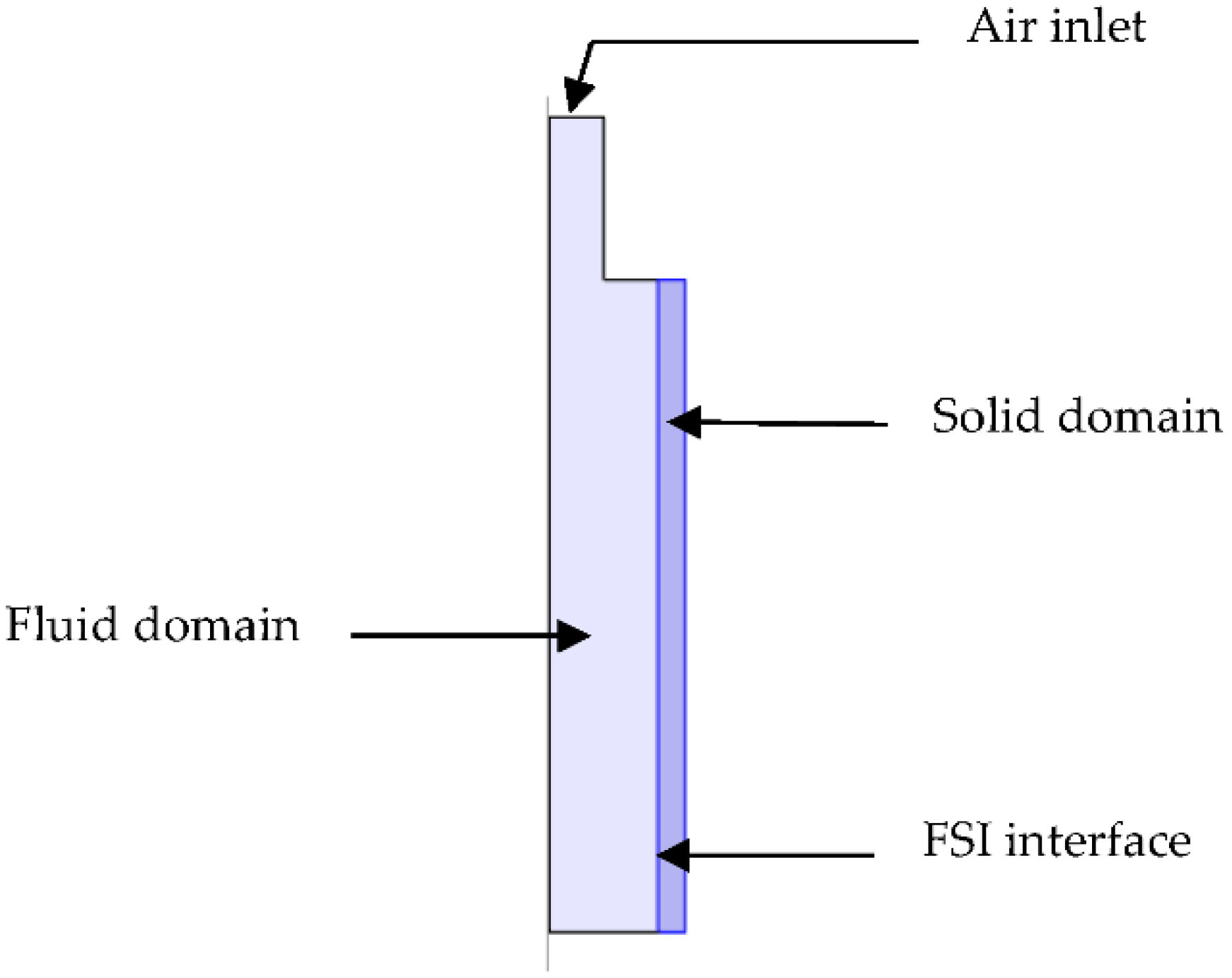
Before implementing an FSI model on a three-dimensional SPA, a two-dimensional FSI study was conducted. The model was built in a two-dimensional frame by implementing the physics closely similar to a PneuNets chamber. The fluid domain, the solid domain, and the FSI interface between fluid and solid are shown in Figure 1. The geometry is axisymmetric to the vertical axis. The two edges of the solid domain were clamped (fixed constraint). The fluid domain was selected for the deforming domain. Upon inlet air pressure, the fluid exerts pressure on the boundary wall (FSI Interface) and the solid domain undergoes deformation (expansion). A silicone-based elastomer named elastosil was used as material for the solid domain, and its nonlinear material behaviour was modelled using the three-parameter Yeoh hyperelastic material model. An inlet air pressure of 0.5 bar was applied in time-steps using a ramp function.
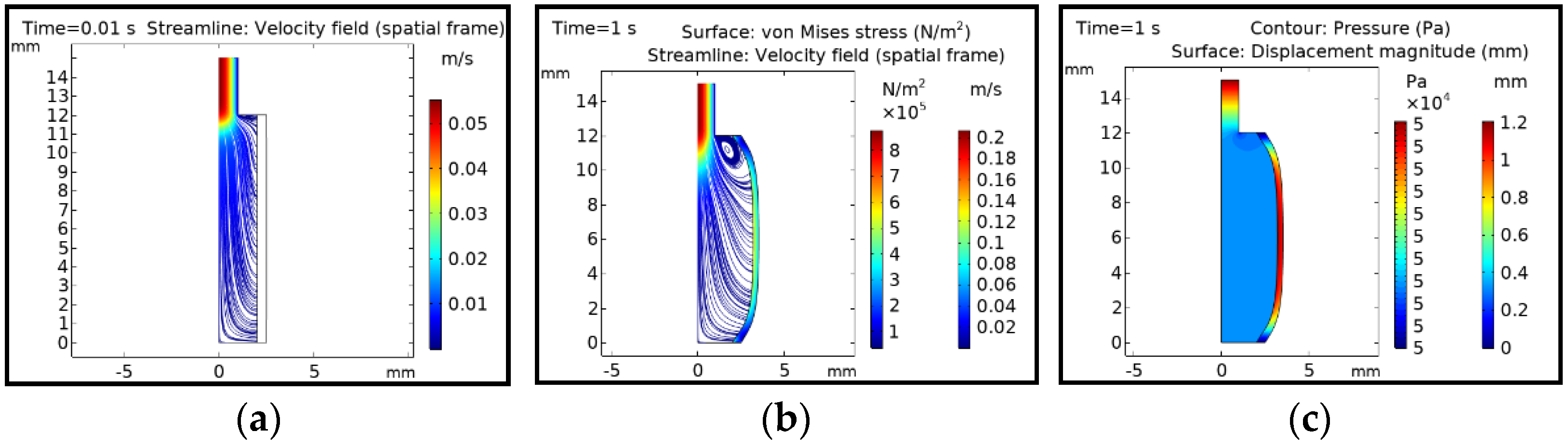
Figure 2 shows the simulation result of the coupled 2D FSI problem. The velocity profile at t = 0.01 s is shown in Figure 2a, in which no deformation of the body can be observed. Figure 2b,c shows the results at t = 1 s, in which an air pressure of 0.5 bar is applied. There was a significant deformation in the solid domain, and the corresponding velocity and stress contours as well as pressure and deformation contours were plotted. This simple 2D study shows the principle of FSI simulation.
2.5. Coupled 3D FSI Modelling and Simulation
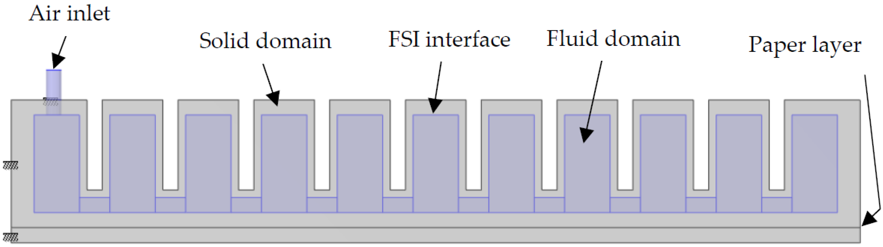
The geometry of the PneuNets bending actuator was imported in COMSOL Multiphysics and modified for the suitability of FSI modelling. The fluid domain inside the actuator was created, and the inlet air supply tube of 2 mm diameter was included in the geometry. The modified PneuNets actuator is shown in Figure 3. It was fixed at the left and top faces of the first chamber. The fluid flow was assumed as incompressible and laminar. Gravity was also taken into account. The model was initially simulated only for gravity using Study Step 1. Once the steady state was reached, the air pressure was gradually applied to the actuator in Study Step 2. The interaction between the chambers upon inflation was taken into account using contact modelling. The paper layer was modelled as a thin elastic layer. The complete modelling procedure is described in detail in Appendix A.
3. Results and Discussion
3.1. Deformation and Comparison with FEM Model
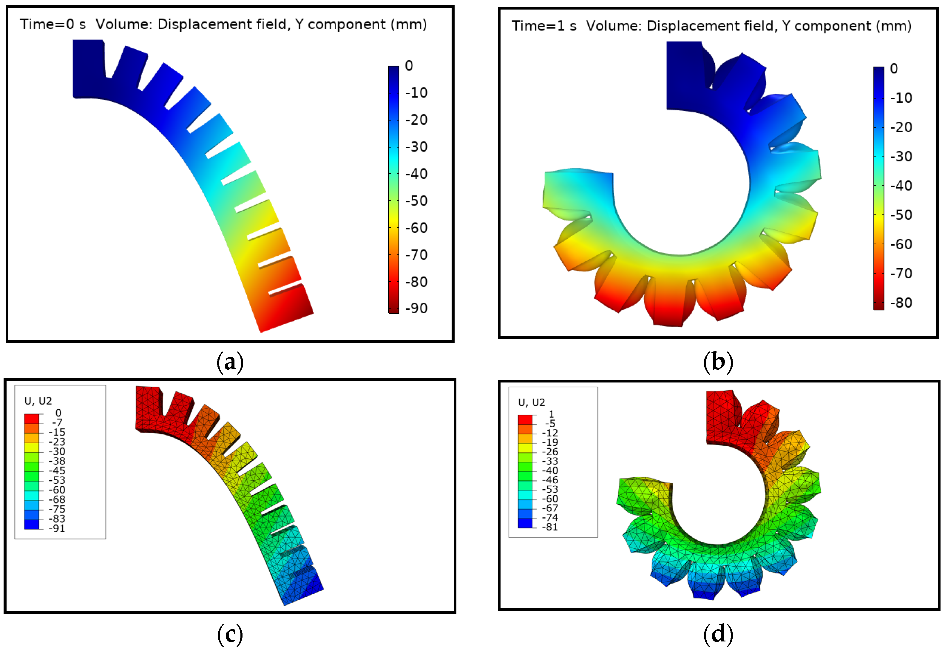
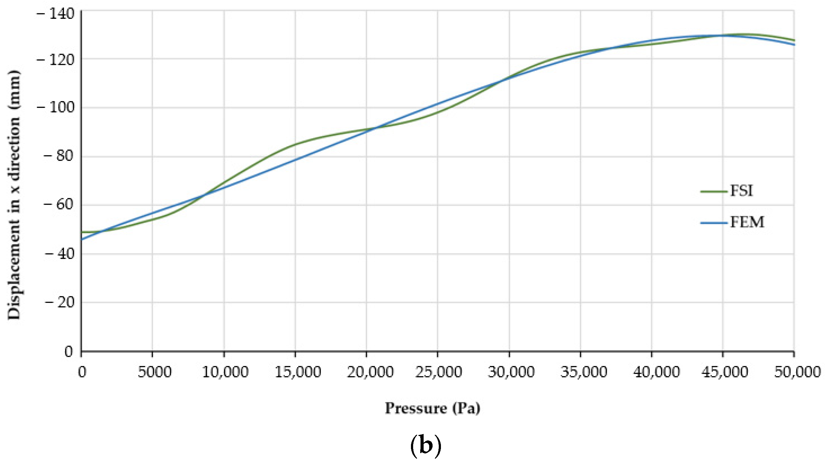
The PneuNets bending actuator was simulated from 0 kPa to 50 kPa. The results of bending deformation of the actuator from the initial to the final state were obtained. The FSI simulation was compared with an FEM counterpart. Since experiments are out of scope of this paper, the simulation model was compared with the FEM model available in [54], which was simulated in the commercial FEM software Abaqus for pressure loads up to 50 kPa, similar to the applied air pressure in the FSI model. It was simulated for the same boundary condition as in the case of FSI. The contour of the bending deformation at the initial state due to gravity and the final state for both FSI and FEM are shown Figure 4. For the comparison, the displacements in x and y direction were taken into account. The right-most actuator tip was selected and its displacement for the applied pressure was retrieved from the FSI model in COMSOL and the FEM model in Abaqus. The comparison of displacements resulting from the two models is shown in Figure 5. At the initial state of 0 kPa, the displacement in y direction started approximately from −80 mm and the displacement in x direction approximately from −46 mm. The negative values in both graphs indicate that the actuator bends downwards (negative y direction) and clockwise (negative x direction). The deformation at the initial state is due to gravity. The comparison shows that the bending behaviour of the FSI model and the FEM model was similar at the initial state and through the complete simulation time. Even though the fluid energy distribution was not the same inside the actuator in the FSI model, the pressure difference between the applied fluid pressure and the pressure distributed on the boundaries of whole fluid domain was not significant, and hence a similar bending behaviour was observed.
The explanation of using an FEM model for comparison is given in Appendix B, with the investigation of the pressure distribution inside the actuator. However, for actuators with high pressurization rates, there is a significant difference in the pressure distribution, which is why this type of comparison is only valid for low applied pressures.
3.2. Initial Time Step Condition
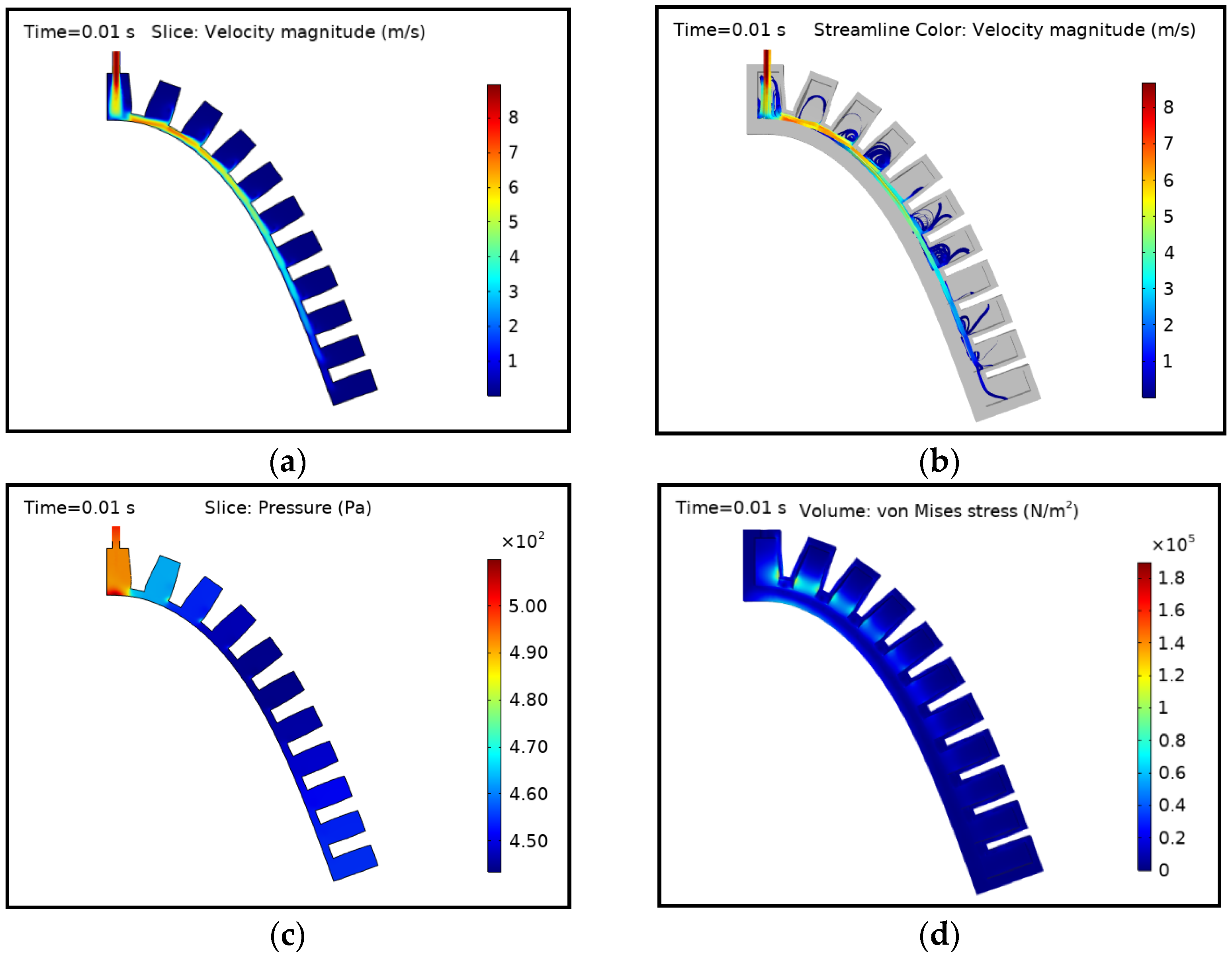
The behaviour of the actuator at the initial time step of 0.01 s is shown in Figure 6. The fluid velocity was higher at the inlet and it propagated until the last chamber of the actuator. The velocity decreased as it reached the last internal chamber, where almost no fluid velocity is present, as seen in (a). The trend was followed by preceding chambers. The middle chambers were not yet fully filled with fluid, as seen in the streamlines in (b). The applied fluid pressure at the inlet at this point was 500 Pa, and the pressure dropped in subsequent chambers. Figure 6c shows that the middle chambers experience a low pressure of nearly 450 Pa as the fluid propagates to the last chamber. The maximum pressure and stress appear in the first chamber since it is in direct contact with the inlet fluid supply hose. Hence, the adjacent walls and surfaces should be designed in such a way that they withstand higher pressures and stresses.
3.3. Middle and Last Time Step Condition
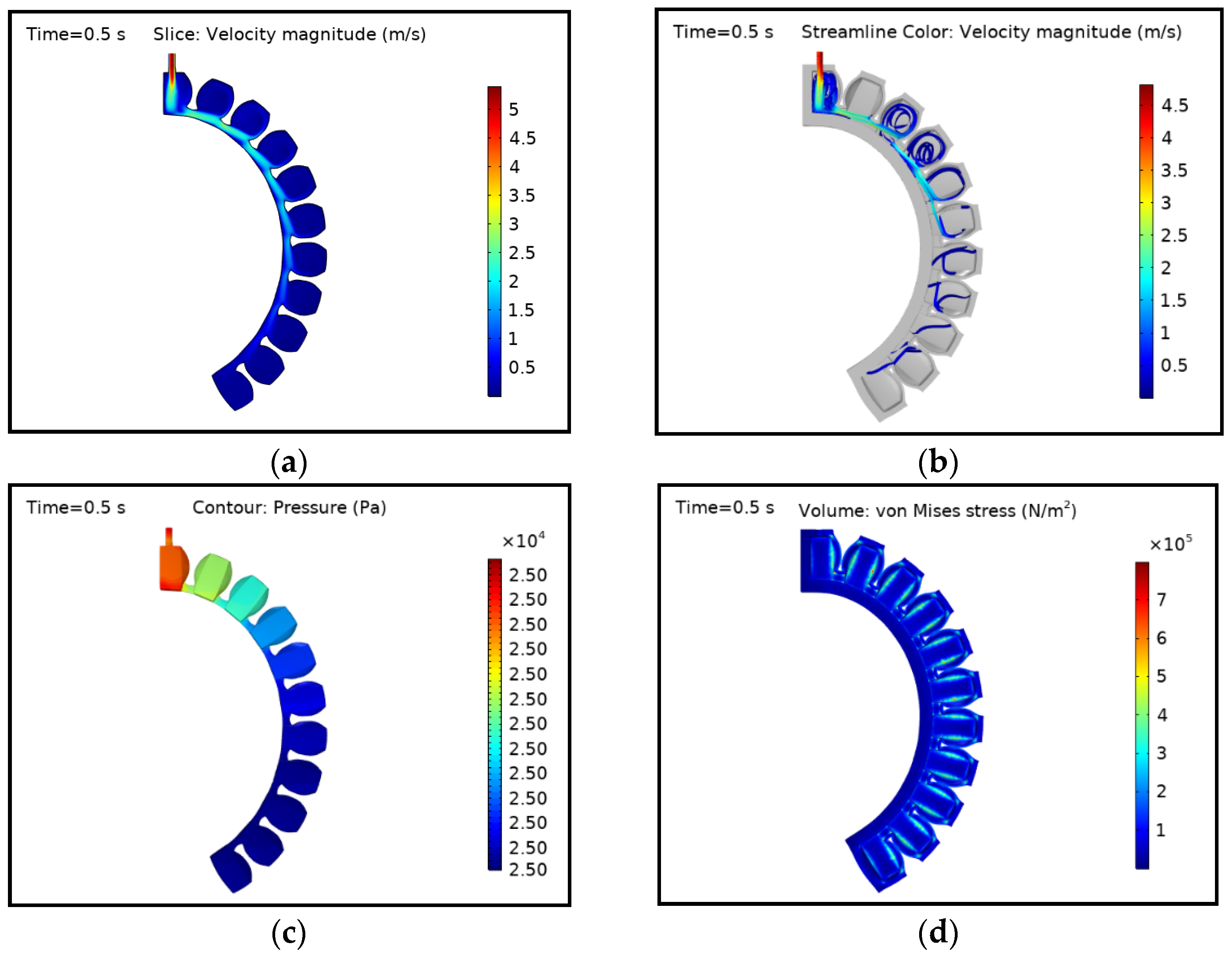
The actuator bended further as the air pressure increased and hence its volume also increased as the chambers inflated. The behaviour of the actuator at a given pressure of 25 kPa is shown in Figure 7. The average velocity of the fluid was smaller than at the initial condition, and the fluid streamlines were not visible in the last chamber, but can be predominantly seen in the middle chambers. The pattern of the fluid streamlines can be closely investigated with respect to bending of the actuator. As the chambers inflate and the actuator bends, the upper walls of the flow channels change and attain the shape close to curvature, resulting in a favouring of the fluid flow in the flow channels. Meanwhile, fluid flowed in x direction in the flow channels and part of it passed through the next immediate chamber as the bending caused the chamber to capture the flow stream. It can be visualised at the edges of the right walls of the chambers from left to right, as shown in Figure 7a. Unlike the initial state, where a pressure drop is observed in the chambers, the pressure of 25 kPa is almost equally distributed among all chambers. This is in accordance with a closed system that, after a certain time, attains equilibrium state.
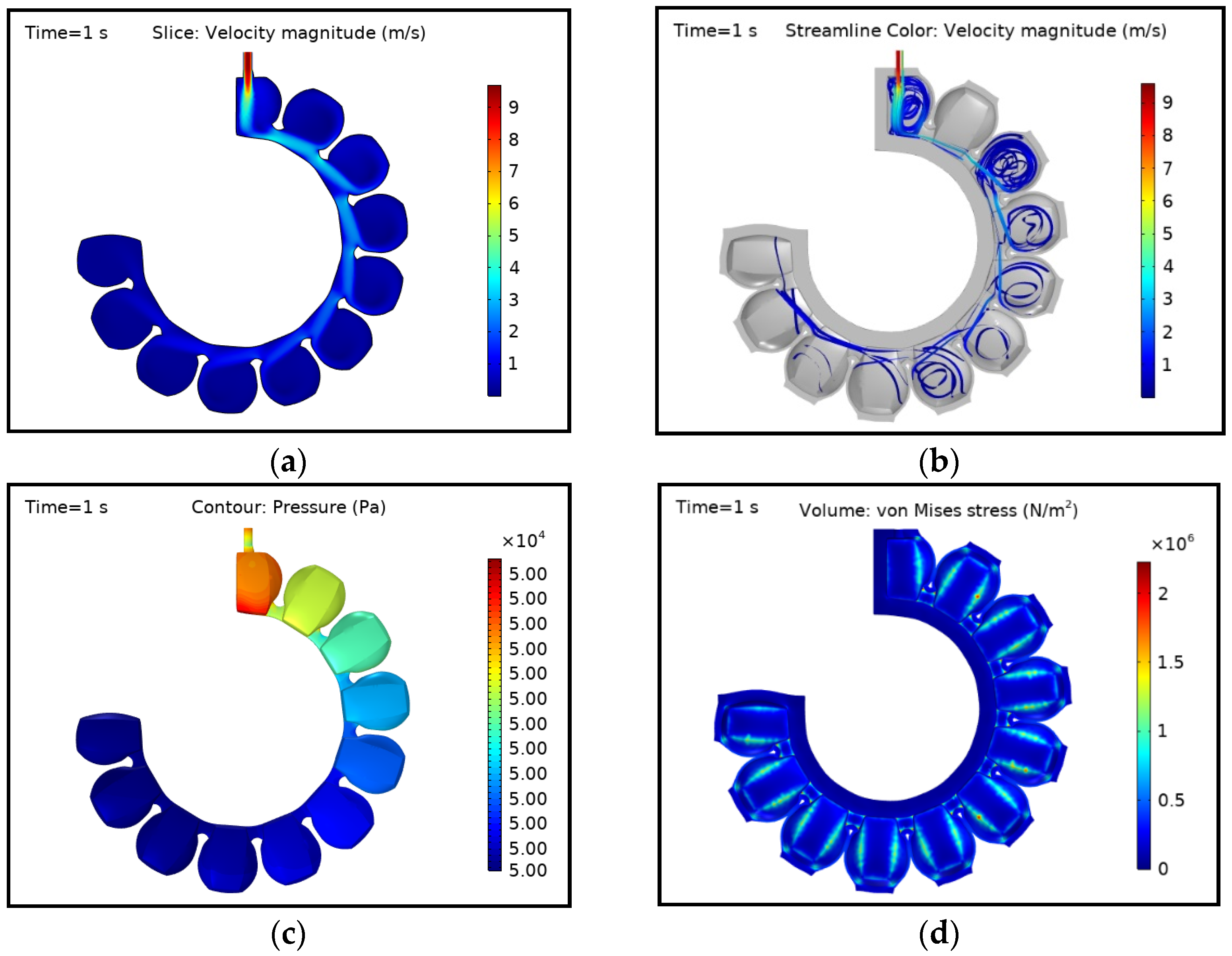
The edges and corners of the flow channels are subjected to more stress. Since pressure energy is consistently supplied into the actuator, which is a closed system, the fluid properties change at different points. The results of the final time step with 50 kPa fluid pressure are shown in Figure 8. The average fluid velocity was relatively higher than the initial state due to more control volume in the actuator, which favours the flow predominantly in the first chamber and flow channels. Similar to the conditions at the middle time step, the streamlines were not observed anymore in the further channels, and the applied pressure of 50 kPa was distributed everywhere inside the domain.
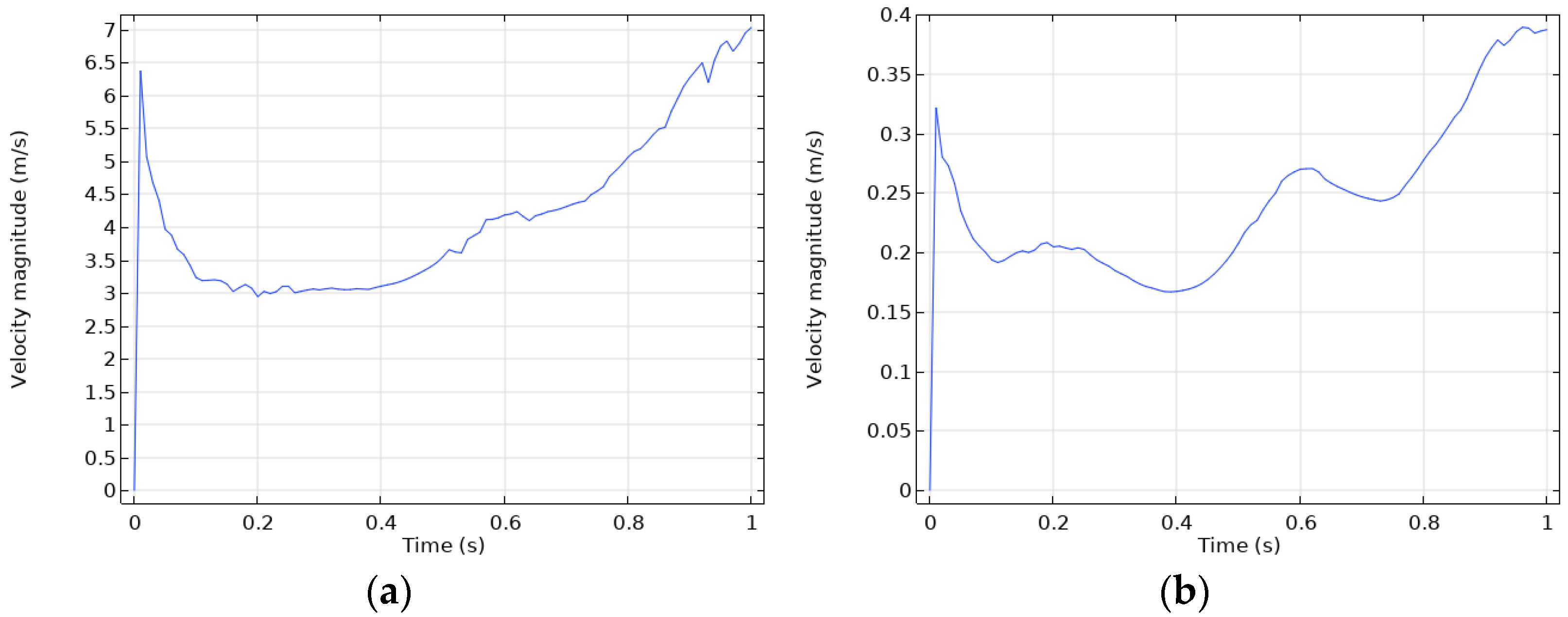
3.4. Average Velocity of Fluid Domain
The average fluid velocity at the inlet and the entire fluid domain of the actuator over the complete simulation time is shown in Figure 9. At the initial time step, the velocity drastically increases, then dips up to 0.2 s (10 kPa), and then it gradually increases up to 1 s (50 kPa). The reason for this behavior is that, initially, there is a void in the chambers and the fluid propagates faster, and later on, since the actuator is a closed system and with continuous fluid supply, the fluid velocity decreases. After that point (0.2 s), as the chambers of the actuator expand, the control volume increases, which causes the fluid velocity to increase further, as long as the chambers inflate. This causes turbulence in the flow. Furthermore, the average fluid velocity of the inlet behaves similar to the whole fluid domain, which interprets the velocity at the inlet as the dominating factor on the average velocity of the fluid domain.
It should be also noted that, since the actuator is a closed system, and that the system boundary is continuously changing due to expansion and bending, fluctuations in the velocity are observed despite the constant rate of pressurization. Since the material properties of the silicone rubber change with respect to the temperature [55], the FSI analysis is useful in investigating the fluid temperature inside soft robots.
4. Conclusions and Outlook
In this work, we developed a fully coupled FSI simulation model for a soft pneumatic actuator and demonstrated the dynamics of fluid flow inside the actuator, as well its structural behaviour. The main contribution of this work is advancing soft robotics in an industrial setting by implementing an FSI simulation model in a commercial software. The simulation model was compared with an FEM model and a similar bending behaviour of the actuator was observed due the negligible difference in the pressure distribution on the walls. Since experiments were not in the scope of this work, as the next step, experiments will be conducted with manufactured soft actuators for the validation of the FSI simulation model. The developed FSI simulation model can be used in different types of SPAs, and the corresponding fluid and structural behaviour can be investigated simultaneously. The fully coupled FSI modelling methodology presented in Appendix A can also be transferred to soft hydraulic actuators with proper adaptations. Furthermore, the developed model is useful for exploring FSI simulation-based design optimization of soft fluidic actuators, especially by investigating the relationship between flow dynamics and deformations. The proposed FSI model can be useful as a design tool for SPAs as a means of investigating the effect of inlet flow parameters, the higher rate of pressurization (Appendix B), and the design parameters of chambers and flow channels on the pressure energy distribution and thus the actuator’s performance. Similar to the FEM analysis performed by Mosadegh et al. [26], the force output of the SPA can also be simulated using FSI analysis, which will be investigated in the future. The modelling of viscoelastic behaviour in the FSI model is also a scope for future work.
The significance of air temperature for materials that are more sensitive to temperature change could be an interesting topic for further investigation. Furthermore, turbulence modelling should be considered in the FSI analysis, as the flow in the actuator is not laminar everywhere. Besides, for 3D printed silicone actuators, the surface structure would affect the flow, which should be investigated as well. Moreover, based on the desired functions of the actuator, the fluid pressure has to be different at different chambers/parts of the actuator at different times. Besides, for control scheme, the rate-dependent behaviour of SPAs provides interesting opportunities [26]. For all these reasons, a sole FEM study cannot be sufficient for the analysis of soft actuators. Moreover, FEM analysis assumes that the pressure load is equally distributed on the walls and is instantly applied, which is not true for all scenarios (Appendix B). Hence, FSI analysis is a potential modelling technique, which should be explored further for the design and development of soft robots. However, a fully coupled FSI analysis is costly and time-consuming, especially for models with turbulence. Hence, further research in the direction of reducing the computing cost by properly making assumptions for the simulation model in order to reduce the complexity and implement novel numerical schemes for solving FSI problems faster would be fruitful to the community.
Author Contributions
Conceptualization, D.M. and A.S.; modelling and simulation, D.M.; writing—original draft preparation, D.M. and A.S.; writing—review and editing, D.M. and A.S.; guidance, A.S.; supervision, A.S. and J.S. All authors have read and agreed to the published version of the manuscript.
Funding
This research received no external funding.
Institutional Review Board Statement
Not applicable.
Informed Consent Statement
Not applicable.
Data Availability Statement
Not applicable.
Acknowledgments
This publication was supported by the funding programme ‘’Open Access Publishing’’ of Hamburg University of Technology (TUHH).
Conflicts of Interest
The authors declare no conflict of interest.
Appendix A
The modelling procedure in COMSOL Multiphysics used in this paper is as follows.
- Required modules in COMSOL: COMSOL Multiphysics Module, Structural Mechanics/MEMS Module, Nonlinear Structural Materials Module, CFD Module, and CAD Import Module
- Space dimension: three-dimensional model
- Physics: fluid–solid interaction
- Study type: stationary (gravity) and time-dependent (air pressure)
- Fluid mechanics: Air is chosen as material. Incompressible and laminar flow are selected. Gravity is included. Walls are treated with no slip condition. Material properties like dynamic viscosity and density of air are considered using a built-in function in COMSOL.
- Solid mechanics:
- ○
- Elastomer: Elastosil is assigned to the top and bottom parts, which is created as user-defined material with a density of 1130 kg/m3. The Yeoh hyperelastic material model is assigned using the model parameters given in Section 2.2.
- ○
- Paper: Paper is assigned to the interface boundary, and linear elastic material behaviour is applied. Paper is created as user defined material with required material properties of density = 750 kg/m3, Poisson’s ratio = 0.2, and Young’s modulus = 6.5 GPa [54].
- ○
- Contacts: The sidewalls of the chambers (except the left sidewall of the first chamber and the right sidewall of the last chamber) are assigned as contact pairs for the deformed configuration. All the left sidewalls are considered as source and the right sidewalls as destination for contact modelling. For the thin paper layer, another contact pair is created for the initial configuration. Contacts are modelled using the penalty condition.
- Moving mesh: The fluid domain is selected as deforming domain under a moving mesh. The Navier–Stokes equations given in (1) and (2) are solved in the deforming domain using Yeoh smoothing with C2 = 10. The prescribed mesh displacement of zero in all directions is applied to the inlet and the wall boundaries of the air supply tube above the first chamber.
- Boundary conditions: An inlet air pressure of 0.5 bar is applied at the inlet boundary. The pressure is applied using the ramp function, gradually increasing the pressure from 0 bar to 0.5 bar from t = 0 s to t = 1 s. The side and top walls of the first chamber are fixed, hence there is no displacement in all directions.
- Gravity is taken into account for the solid domain, and it acts in negative y direction.
- Fluid–structure interaction: The fluid domain is selected as deforming domain under a moving mesh and the walls of the fluid chambers are automatically assigned as the interface for fluid and solid. The fully coupled solver is selected for simulating fluid and solid domains.
- Mesh: The physics-controlled mesh is selected. The fine mesh is created predominantly with tetrahedral elements. The mesh is generated specifically in each domain and FSI interface. The total number of mesh elements is 1,022,609, in which 598,947 elements represent the fluid domain and are calibrated for fluid mechanics and 311,810 elements represent the solid domains. The minimum element quality based on skewness is 0.06.
- Study: Two study steps are implemented. Study Step 1 denotes a stationary study, which solves the model for gravity. Regarding this, the parameter t is defined with value zero in global definition. Study Step 2 denotes the time-dependent study, in which the inlet pressure is applied in time steps. The time steps are given as 0, 0.01, and 1 s. The inlet pressure increases for each time step by 500 Pa.
- Solver: The segregated solver is selected for the time-dependent study. Compared to the fully coupled solver, the segregated solver approach requires less memory and computation time.
- Cluster specifications: The model is computed on 24 cores running at 2.5 GHz. It takes 18 h and 43 min to compute.
Appendix B
The motivation of the work states that FEM cannot be accurate in all scenarios. Therefore, the FSI can be compared with FEM and it can be shown how much the result deviates. For the FSI model discussed in the Section 3, the bending deformation behaviour is similar to the FEM model (Figure 5a,b). The reason for this similar bending behaviour is discussed here with respect to the difference between the applied fluid pressure and the pressure distribution inside the fluid boundaries. This effect is illustrated in Figure A1.
Figure A1.
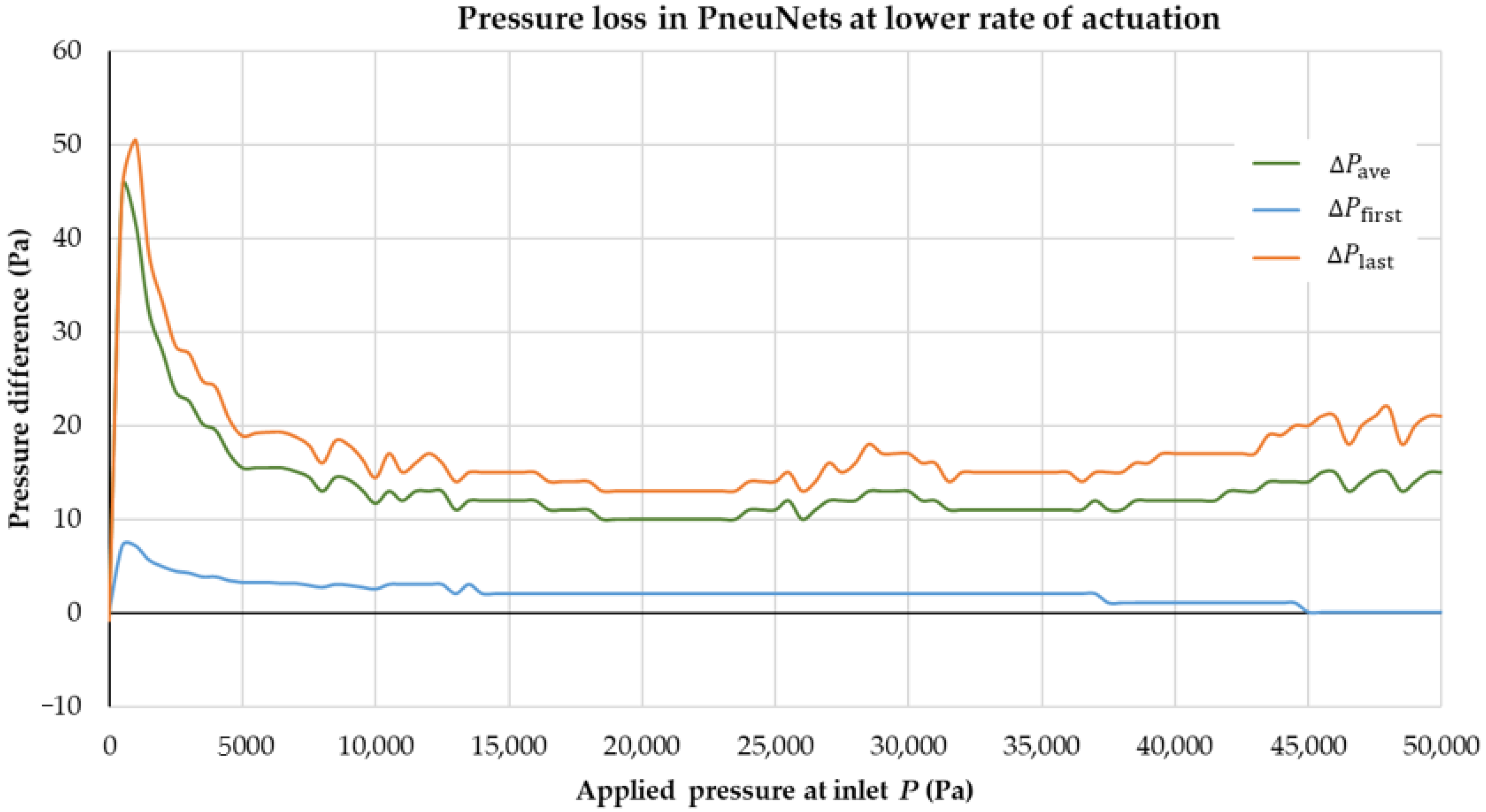
Pressure difference in the actuator at lower rates of pressurization: P is the applied air pressure at the inlet; ΔPave is the difference between P and the average fluid pressure distributed on the boundaries of the fluid domain; ΔPfirst is the difference between P and the average pressure distributed on the walls of the first chamber; ΔPlast is the difference between P and the average pressure distributed on the walls of the last chamber.
Figure A1.
Pressure difference in the actuator at lower rates of pressurization: P is the applied air pressure at the inlet; ΔPave is the difference between P and the average fluid pressure distributed on the boundaries of the fluid domain; ΔPfirst is the difference between P and the average pressure distributed on the walls of the first chamber; ΔPlast is the difference between P and the average pressure distributed on the walls of the last chamber.

The reason for the similar displacement behaviour in Figure 5 is due to a less magnitude of pressure loss, which is illustrated in Figure A1. It shows the differences from the applied air pressure at the inlet to the average pressure distributed on the walls of the first chamber, the walls of the last chamber, and the boundaries of the whole fluid domain of the actuator. Only at the initial time steps is the pressure difference (ΔPlast = 50 Pa) relatively larger than in the later time steps. Nevertheless, the magnitude of the pressure difference is not significant (ΔPave predominantly lies between 10 Pa and 20 Pa, and the highest value of ΔPlast is 50 Pa at the initial time steps). Therefore, there is no significant deviation in the bending behaviour of the actuator between the FSI and FEM models in the initial time steps as well as throughout the simulation time. The chambers of the actuator at this rate of pressurization inflate uniformly. Therefore, in this case, a comparison of the FSI model with the FEM model is acceptable and is treated as verification, as there are no significant pressure changes from the applied pressure to the walls inside the actuator.
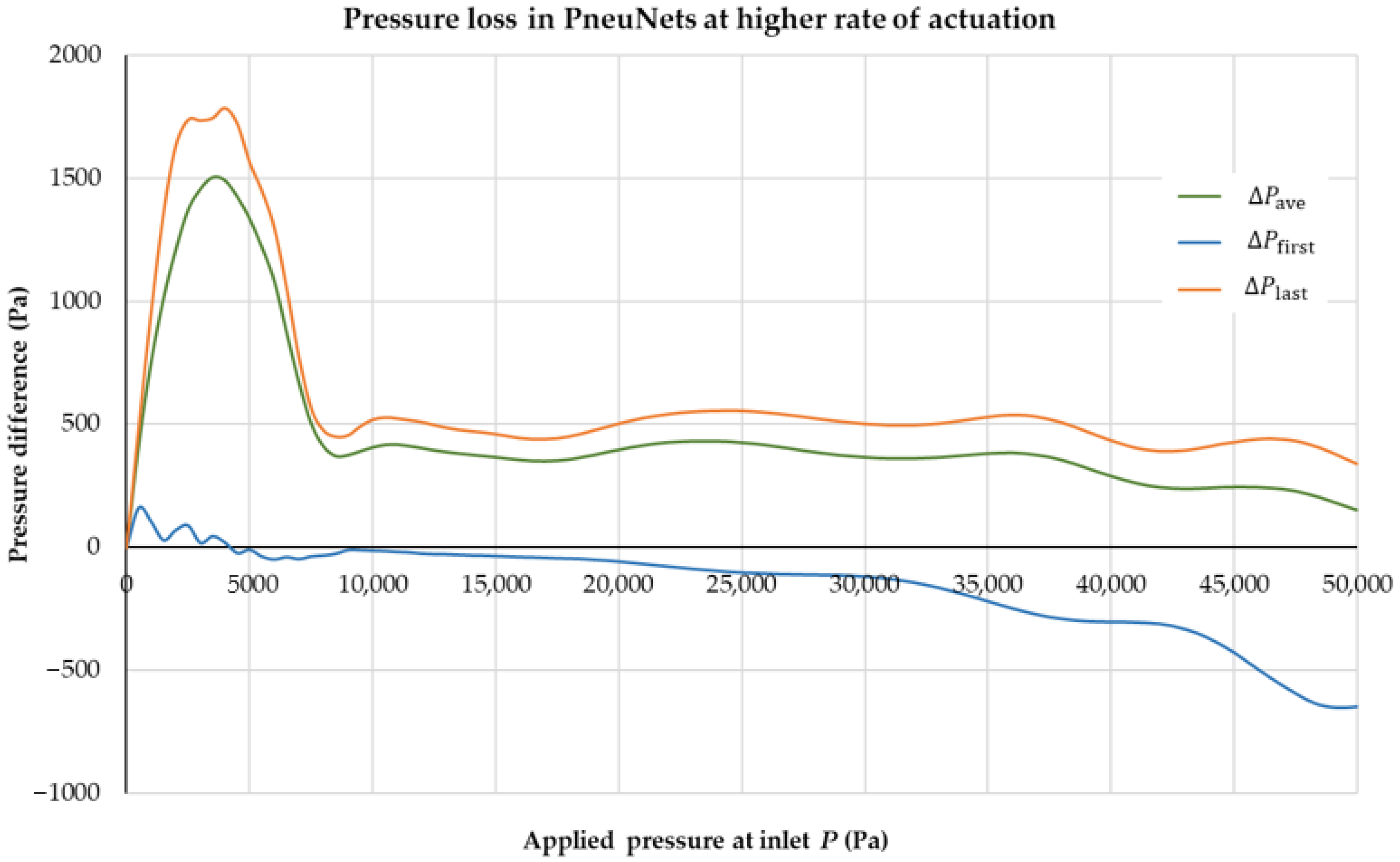
However, as mentioned in the motivation of this work, the pressure is not equally applied to the walls of the actuator in all scenarios. For example, at higher rates of pressurization, the bending behaviour is different compared to lower rates of pressurization, as discussed in [26]. This phenomenon is investigated on the SPA using the FSI model. Here, the air pressure is applied from 0 Pa to 50,000 Pa at the time range from 0 s to 0.1 s. Note that, in this study, gravity has not been taken into account.
The differences from the applied air pressure at the inlet to the average pressure distributed on the walls of the first chamber, the walls of the last chamber, and the boundaries of the whole fluid domain of the actuator are shown in Figure A2. Unlike the model with a slower rate of pressurization, the pressure loss at the initial state (maximum value of ΔPave = 1500 Pa), as well as throughout the simulation time (ΔPave predominantly lies in the range above 350 Pa), is significant for higher rates of pressurization. It also shows that the pressure distributed on the walls of the first chamber is higher than the applied air pressure at the inlet and hence the pressure difference (ΔPfirst) shows negative values in Figure A2.
Figure A2.
Pressure difference in the actuator at higher rates of pressurization: P is the applied air pressure at the inlet; ΔPave is the difference between P and the average fluid pressure distributed on the boundaries of the fluid domain; ΔPfirst is the difference between P and the average pressure distributed on the walls of the first chamber; ΔPlast is the difference between P and the average pressure distributed on the walls of the last chamber.

The above analysis illustrates that the pressure is not equally distributed inside the actuator for higher rates of pressurization. As a reference, the contours of the pressure energy distribution on the walls of the actuator at higher rates of pressurization is presented in Figure A3. The bending behaviour of the actuator at higher rates of pressurization is different from the one at lower rates of pressurization. The last and the preceding chambers inflate faster than the chambers near to the inlet. The chambers are inflated uniformly at lower rates of pressurization (Section 3) and nonuniformly at higher rates of pressurization, as shown in Figure A3. Thus, the assumption made in the FEM model that the pressure is uniformly applied on the wall cannot be valid for all scenarios. Therefore, the FSI model is a useful tool in investigating the behaviour of SPAs where the pressure irregularities inside the actuator are significant.
Figure A3.
Pressure distribution on the boundaries of the chambers in the PneuNets bending actuator at higher rates of pressurization: (a) At 500 Pa inlet pressure; (b) At 5000 Pa inlet pressure; (c) At 12,500 Pa inlet pressure; (d) At 25,000 Pa inlet pressure; (e) At 37,500 Pa inlet pressure; (f) At 50,000 Pa inlet pressure.

References
- Laschi, C.; Mazzolai, B.; Cianchetti, M. Soft robotics: Technologies and systems pushing the boundaries of robot abilities. Sci. Robot. 2016, 1, eaah3690. [Google Scholar] [CrossRef] [PubMed] [Green Version]
- Marchese, A.D.; Katzschmann, R.K.; Rus, D. Whole arm planning for a soft and highly compliant 2D robotic manipulator. In Proceedings of the 2014 IEEE/RSJ International Conference on Intelligent Robots and Systems, Chicago, IL, USA, 14–18 September 2014; pp. 554–560. [Google Scholar]
- Burgner-Kahrs, J.; Rucker, D.C.; Choset, H. Continuum robots for medical applications: A survey. IEEE Trans. Robot. 2015, 31, 1261–1280. [Google Scholar] [CrossRef]
- Kim, D.H.; Heo, S.H.; Park, H.S. Biomimetic finger extension mechanism for soft wearable hand rehabilitation devices. In Proceedings of the 2017 International Conference on Rehabilitation Robotics (ICORR), London, UK, 17–20 July 2017; pp. 1326–1330. [Google Scholar]
- Maeder-York, P.; Clites, T.; Boggs, E.; Neff, R.; Polygerinos, P.; Holland, D.; Stirling, L.; Galloway, K.; Wee, C.; Walsh, C. Biologically inspired soft robot for thumb rehabilitation. J. Med. Devices 2014, 8, 020933. [Google Scholar] [CrossRef] [Green Version]
- Polygerinos, P.; Lyne, S.; Wang, Z.; Nicolini, L.F.; Mosadegh, B.; Whitesides, G.M.; Walsh, C.J. Towards a soft pneumatic glove for hand rehabilitation. In Proceedings of the 2013 IEEE/RSJ International Conference on Intelligent Robots and Systems, Tokyo, Japan, 3–7 November 2013; pp. 1512–1517. [Google Scholar]
- Villoslada, A.; Flores, A.; Copaci, D.; Blanco, D.; Moreno, L. High-displacement flexible shape memory alloy actuator for soft wearable robots. Robot. Auton. Syst. 2015, 73, 91–101. [Google Scholar] [CrossRef]
- Copaci, D.; Cano, E.; Moreno, L.; Blanco, D. New design of a soft robotics wearable elbow exoskeleton based on shape memory alloy wire actuators. Appl. Bionics Biomech. 2017, 2017, 1–11. [Google Scholar] [CrossRef] [PubMed] [Green Version]
- Oguntosin, V.; Harwin, W.S.; Kawamura, S.; Nasuto, S.J.; Hayashi, Y. Development of a wearable assistive soft robotic device for elbow rehabilitation. In Proceedings of the 2015 IEEE International Conference on Rehabilitation Robotics (ICORR), Singapore, 11–14 August 2015; pp. 747–752. [Google Scholar]
- Manfredi, L.; Capoccia, E.; Ciuti, G.; Cuschieri, A. A Soft Pneumatic Inchworm Double balloon (SPID) for colonoscopy. Sci. Rep. 2019, 9, 1–9. [Google Scholar] [CrossRef] [Green Version]
- Jianfei, C.; Xingsong, W. Conception of a tendon-sheath and pneumatic system driven soft rescue robot. In Robot Intelligence Technology and Applications 3; Springer: Cham, Switzerland, 2015; pp. 475–481. [Google Scholar]
- Tolley, M.T.; Shepherd, R.F.; Mosadegh, B.; Galloway, K.C.; Wehner, M.; Karpelson, M.; Wood, R.J.; Whitesides, G.M. A resilient, untethered soft robot. Soft Robot. 2014, 1, 213–223. [Google Scholar] [CrossRef]
- Shintake, J.; Cacucciolo, V.; Floreano, D.; Shea, H. Soft robotic grippers. Adv. Mater. 2018, 30, 1707035. [Google Scholar] [CrossRef] [Green Version]
- Dong, W.; Wang, Y.; Zhou, Y.; Bai, Y.; Ju, Z.; Guo, J.; Gu, G.; Bai, K.; Ouyang, G.; Chen, S.; et al. Soft human–machine interfaces: Design, sensing and stimulation. Int. J. Intell. Robot. Appl. 2018, 2, 313–338. [Google Scholar] [CrossRef] [Green Version]
- Serchi, F.G.; Arienti, A.; Baldoli, I.; Laschi, C. An elastic pulsed-jet thruster for Soft Unmanned Underwater Vehicles. In Proceedings of the 2013 IEEE International Conference on Robotics and Automation, Karlsruhe, Germany, 6–10 May 2013; pp. 5103–5110. [Google Scholar]
- Hines, L.; Petersen, K.; Lum, G.Z.; Sitti, M. Soft actuators for small-scale robotics. Adv. Mater. 2017, 29, 1603483. [Google Scholar] [CrossRef]
- Boyraz, P.; Runge, G.; Raatz, A. An overview of novel actuators for soft robotics. Actuators 2018, 7, 48. [Google Scholar] [CrossRef] [Green Version]
- Zhang, J.; Sheng, J.; O’Neill, C.T.; Walsh, C.J.; Wood, R.J.; Ryu, J.H.; Desai, J.P.; Yip, M.C. Robotic artificial muscles: Current progress and future perspectives. IEEE Trans. Robot. 2019, 35, 761–781. [Google Scholar] [CrossRef]
- Adami, M.; Seibel, A. On-board pneumatic pressure generation methods for soft robotics applications. Actuators 2019, 8, 2. [Google Scholar] [CrossRef] [Green Version]
- Seibel, A.; Schiller, L. Systematic engineering design helps creating new soft machines. Robot. Biomim. 2018, 5, 5. [Google Scholar] [CrossRef] [PubMed] [Green Version]
- Manfredi, L.; Putzu, F.; Guler, S.; Huan, Y.; Cuschieri, A. 4 DOFs hollow soft pneumatic actuator–HOSE. Mater. Res. Express 2019, 6, 045703. [Google Scholar] [CrossRef] [Green Version]
- Suzumori, K.; Iikura, S.; Tanaka, H. Flexible microactuator for miniature robots. In Proceedings of the IEEE Micro Electro Mechanical Systems, Nara, Japan, 30 December 1990–2 January 1991; pp. 204–209. [Google Scholar]
- Suzumori, K.; Iikura, S.; Tanaka, H. Development of flexible microactuator and its applications to robotic mechanisms. In Proceedings of the 1991 IEEE International Conference on Robotics and Automation, Sacramento, CA, USA, 9–11 April 1991; pp. 1622–1627. [Google Scholar]
- Manfredi, L.; Yue, L.; Zhang, J.; Cuschieri, A. A 4 DOFs variable stiffness soft module. In Proceedings of the 2018 IEEE International Conference on Soft Robotics (RoboSoft), Livorno, Italy, 24–28 April 2018; pp. 94–99. [Google Scholar]
- Cianchetti, M.; Laschi, C.; Menciassi, A.; Dario, P. Biomedical applications of soft robotics. Nat. Rev. Mater. 2018, 3, 143–153. [Google Scholar] [CrossRef]
- Mosadegh, B.; Polygerinos, P.; Keplinger, C.; Wennstedt, S.; Shepherd, R.F.; Gupta, U.; Shim, J.; Bertoldi, K.; Walsh, C.J.; Whitesides, G.M. Pneumatic networks for soft robotics that actuate rapidly. Adv. Funct. Mater. 2014, 24, 2163–2170. [Google Scholar] [CrossRef]
- Polygerinos, P.; Wang, Z.; Overvelde, J.T.; Galloway, K.C.; Wood, R.J.; Bertoldi, K.; Walsh, C.J. Modeling of soft fiber-reinforced bending actuators. IEEE Trans. Robot. 2015, 31, 778–789. [Google Scholar] [CrossRef] [Green Version]
- Connolly, F.; Walsh, C.J.; Bertoldi, K. Automatic design of fiber-reinforced soft actuators for trajectory matching. Proc. Natl. Acad. Sci. USA 2017, 114, 51–56. [Google Scholar] [CrossRef] [Green Version]
- Yang, C.; Kang, R.; Branson, D.T.; Chen, L.; Dai, J.S. Kinematics and statics of eccentric soft bending actuators with external payloads. Mech. Mach. Theory 2019, 139, 526–541. [Google Scholar] [CrossRef]
- Gu, G.; Wang, D.; Ge, L.; Zhu, X. Analytical Modeling and Design of Generalized PneuNet Soft Actuators with Three-Dimensional Deformations. Soft Robot. 2020. [Google Scholar] [CrossRef]
- Breitman, P.; Matia, Y.; Gat, A.D. Fluid mechanics of pneumatic soft robots. Soft Robot. 2020. [Google Scholar] [CrossRef] [PubMed]
- Wikipedia. Fluid-Structure Interaction. Available online: https://en.wikipedia.org/wiki/Fluid%E2%80%93structure_interaction (accessed on 6 July 2021).
- Moon, D.H.; Shin, S.H.; Na, J.B.; Han, S.Y. Fluid-structure interaction based on meshless local Petrov-Galerkin method for worm soft robot Analysis. Int. J. Precis. Eng. Manuf. Green Technol. 2020, 7, 727–742. [Google Scholar] [CrossRef]
- Gul, J.Z.; Kim, K.H.; Lim, J.H.; Doh, Y.H.; Choi, K.H. FSI modeling of frog inspired soft robot embedded with ALD encapsulated flex sensor for underwater synchronous swim. In Proceedings of the 2017 IEEE International Symposium on Robotics and Intelligent Sensors (IRIS), Ottawa, ON, Canada, 5–7 October 2017; pp. 255–259. [Google Scholar]
- Bao, G.; Fang, H.; Chen, L.; Wan, Y.; Xu, F.; Yang, Q.; Zhang, L. Soft robotics: Academic insights and perspectives through bibliometric analysis. Soft Robot. 2018, 5, 229–241. [Google Scholar] [CrossRef] [PubMed]
- COMSOL Application Gallery. Fluid-Structure Interaction. Available online: https://www.comsol.com/model/fluid-structure-interaction-361 (accessed on 3 May 2021).
- Multiphysics Cyclopedia. Fluid-Structure Interaction. Available online: https://www.comsol.com/multiphysics/fluid-structure-interaction (accessed on 5 May 2021).
- Fras, J.; Glowka, J.; Althoefer, K. Instant soft robot: A simple recipe for quick and easy manufacturing. In Proceedings of the 2020 3rd IEEE International Conference on Soft Robotics (RoboSoft), New Haven, CT, USA, 15 May–15 July 2020; pp. 482–488. [Google Scholar]
- Gul, J.Z.; Sajid, M.; Rehman, M.M.; Siddiqui, G.U.; Shah, I.; Kim, K.H.; Lee, J.W.; Choi, K.H. 3D printing for soft robotics—A review. Sci. Technol. Adv. Mater. 2018, 19, 243–262. [Google Scholar] [CrossRef] [PubMed] [Green Version]
- Wallin, T.J.; Pikul, J.; Shepherd, R.F. 3D printing of soft robotic systems. Nat. Rev. Mater. 2018, 3, 84–100. [Google Scholar] [CrossRef]
- Gent, A.N. Engineering with Rubber: How to Design Rubber Components, 2nd ed.; Hanser: Munich, Germany, 2001. [Google Scholar]
- Mullins, L. Effect of stretching on the properties of rubber. Rubber Chem. Technol. 1948, 21, 281–300. [Google Scholar] [CrossRef]
- Cantournet, S.; Desmorat, R.; Besson, J. Mullins effect and cyclic stress softening of filled elastomers by internal sliding and friction thermodynamics model. Int. J. Solids Struct. 2009, 46, 2255–2264. [Google Scholar] [CrossRef]
- Ali, A.; Hosseini, M.; Sahari, B.B. A review of constitutive models for rubber-like materials. Am. J. Eng. Appl. Sci. 2010, 3, 232–239. [Google Scholar] [CrossRef] [Green Version]
- Treloar, L.R.G. The elasticity of a network of long-chain molecules. i. Trans. Faraday Soc. 1943, 39, 36–41. [Google Scholar] [CrossRef]
- Treloar, L.R.G. The elasticity of a network of long-chain molecules. ii. Trans. Faraday Soc. 1943, 39, 241–246. [Google Scholar] [CrossRef]
- Rivlin, R. Large elastic deformations of isotropic materials. i. Fundamental concepts. Philos. Trans. R. Soc. Lond. Ser. A Math. Phys. Sci. 1948, 240, 459–490. [Google Scholar]
- Rivlin, R.S. Large elastic deformations of isotropic materials. iv. Further developments of the general theory. Philos. Trans. R. Soc. Lond. Ser. A Math. Phys. Sci. 1948, 241, 379–397. [Google Scholar]
- Ogden, R.W. Large deformation isotropic elasticity–on the correlation of theory and experiment for incompressible rubberlike solids. Proc. R. Soc. London. A. Math. Phys. Sci. 1972, 326, 565–584. [Google Scholar] [CrossRef]
- Yeoh, O.H. Some forms of the strain energy function for rubber. Rubber Chem. Technol. 1993, 66, 754–771. [Google Scholar] [CrossRef]
- Arruda, E.M.; Boyce, M.C. A three-dimensional constitutive model for the large stretch behavior of rubber elastic materials. J. Mech. Phys. Solids 1993, 41, 389–412. [Google Scholar] [CrossRef] [Green Version]
- Behroozi, M.; Olatunbosun, O.A.; Ding, W. Finite element analysis of aircraft tyre–effect of model complexity on tyre performance characteristics. Mater. Des. 2012, 35, 810–819. [Google Scholar] [CrossRef]
- Xavier, M.S.; Fleming, A.J.; Yong, Y.K. Finite element modeling of soft fluidic actuators: Overview and recent developments. Adv. Intell. Syst. 2021, 3, 2000187. [Google Scholar] [CrossRef]
- Soft Robotics Toolkit. PneuNets Modeling. Available online: https://softroboticstoolkit.com/book/pneunets-modeling (accessed on 5 September 2020).
- Utkan, D.; Maruthavanan, D.; Schimanowski, A.; Seibel, A. Compression behavior of typical silicone rubbers for soft robotic applications at elevated temperatures. In Proceedings of the 2021 4th IEEE International Conference on Soft Robotics (RoboSoft), New Haven, CT, USA, 12–16 April 2021; pp. 539–542. [Google Scholar]
Figure 1.
Coupled 2D FSI problem.

Figure 2.
Simulation results of the coupled 2D FSI problem: (a) Fluid velocity streamline at the initial time step; (b) Fluid velocity streamline and solid stress at the final time step; (c) Fluid pressure and solid deformation at the final time step.
Figure 2.
Simulation results of the coupled 2D FSI problem: (a) Fluid velocity streamline at the initial time step; (b) Fluid velocity streamline and solid stress at the final time step; (c) Fluid pressure and solid deformation at the final time step.

Figure 3.
Domain details of the PneuNets bending actuator used in FSI modelling.

Figure 4.
Deformation comparison of the PneuNets bending actuator from the FSI and FEM simulation models: (a) Initial deformation from the FSI model due to gravity at 0 kPa pressure; (b) Final deformation from the FSI model at 50 kPa pressure; (c) Initial deformation from the FEM model due to gravity at 0 kPa pressure; (d) Final deformation from the FEM model at 50 kPa pressure.

Figure 5.
Comparison of the displacement path measured at the actuator tip from the FSI and FEM simulation models: (a) Pressure vs. displacement in y direction; (b) Pressure vs. displacement in x direction.
Figure 5.
Comparison of the displacement path measured at the actuator tip from the FSI and FEM simulation models: (a) Pressure vs. displacement in y direction; (b) Pressure vs. displacement in x direction.


Figure 6.
FSI simulation results of the PneuNets bending actuator at the initial time step of 0.01 s: (a) Velocity magnitude at the mid surface; (b) Flow streamlines with velocity magnitude (cross sectional view); (c) Pressure distribution in the fluid domain; (d) Stress distribution in the actuator (cross sectional view).

Figure 7.
FSI simulation results of the PneuNets bending actuator at the middle time step of 0.5 s: (a) Velocity magnitude at the mid surface; (b) Flow streamlines with velocity magnitude (cross sectional view); (c) Pressure distribution in the fluid domain; (d) Stress distribution in the actuator (cross sectional view).

Figure 8.
FSI simulation results of the PneuNets bending actuator at the final time step of 1 s: (a) Velocity magnitude at the mid surface; (b) Flow streamlines with velocity magnitude (cross sectional view); (c) Pressure distribution in the fluid domain; (d) Stress distribution in the actuator (cross sectional view).

Figure 9.
Average velocity plot for the complete simulation: (a) Velocity plot at the inlet boundary; (b) Velocity plot for the whole fluid domain.
Figure 9.
Average velocity plot for the complete simulation: (a) Velocity plot at the inlet boundary; (b) Velocity plot for the whole fluid domain.


Table 1.
Material properties of typical silicone-based elastomers in soft robotics applications.
| Sylgard | Elastosil | Ecoflex | |
|---|---|---|---|
| Manufacturer | Dow Corning | Wacker Chemie | Smooth-On |
| Type | 184 | M4601 | 00–30 |
| Colour | transparent | reddish brown | translucent |
| Shore hardness | 50 A | 28 A | 00–30 |
| Tensile strength | 6.76 MPa | 6.50 MPa | 1.38 MPa |
| Density | 1.04 g/cm3 | 1.13 g/cm3 | 1.07 g/cm3 |
| Elongation at break | 150% | 700% | 900% |
Publisher’s Note: MDPI stays neutral with regard to jurisdictional claims in published maps and institutional affiliations. |
© 2021 by the authors. Licensee MDPI, Basel, Switzerland. This article is an open access article distributed under the terms and conditions of the Creative Commons Attribution (CC BY) license (https://creativecommons.org/licenses/by/4.0/).
Share and Cite
MDPI and ACS Style
Maruthavanan, D.; Seibel, A.; Schlattmann, J. Fluid-Structure Interaction Modelling of a Soft Pneumatic Actuator. Actuators 2021, 10, 163. https://doi.org/10.3390/act10070163
AMA Style
Maruthavanan D, Seibel A, Schlattmann J. Fluid-Structure Interaction Modelling of a Soft Pneumatic Actuator. Actuators. 2021; 10(7):163. https://doi.org/10.3390/act10070163
Chicago/Turabian StyleMaruthavanan, Duraikannan, Arthur Seibel, and Josef Schlattmann. 2021. "Fluid-Structure Interaction Modelling of a Soft Pneumatic Actuator" Actuators 10, no. 7: 163. https://doi.org/10.3390/act10070163
Note that from the first issue of 2016, this journal uses article numbers instead of page numbers. See further details here.