Article

siEDM: An Efficient String Index and Search Algorithm for Edit Distance with Moves

1
Graduate School of Computer Science and Systems Engineering, Kyushu Institute of Technology, 680-4 Kawazu, Iizuka-shi, Fukuoka 820-8502, Japan
2
Computer Centre, Gakushuin University, 1-5-1 Mejiro, Toshima-ku, Tokyo 171-8588, Japan
3
PRESTO, Japan Science and Technology Agency, 4-1-8 Honcho, Kawaguchi-shi, Saitama 332-0012, Japan
*
Author to whom correspondence should be addressed.
Algorithms 2016, 9(2), 26; https://doi.org/10.3390/a9020026
Submission received: 25 November 2015 / Revised: 8 April 2016 / Accepted: 11 April 2016 / Published: 15 April 2016

Abstract

:
Although several self-indexes for highly repetitive text collections exist, developing an index and search algorithm with editing operations remains a challenge. Edit distance with moves (EDM) is a string-to-string distance measure that includes substring moves in addition to ordinal editing operations to turn one string into another. Although the problem of computing EDM is intractable, it has a wide range of potential applications, especially in approximate string retrieval. Despite the importance of computing EDM, there has been no efficient method for indexing and searching large text collections based on the EDM measure. We propose the first algorithm, named string index for edit distance with moves (siEDM), for indexing and searching strings with EDM. The siEDM algorithm builds an index structure by leveraging the idea behind the edit sensitive parsing (ESP), an efficient algorithm enabling approximately computing EDM with guarantees of upper and lower bounds for the exact EDM. siEDM efficiently prunes the space for searching query strings by the proposed method, which enables fast query searches with the same guarantee as ESP. We experimentally tested the ability of siEDM to index and search strings on benchmark datasets, and we showed siEDM’s efficiency.

1. Introduction

Vast amounts of text data are created, replicated, and modified with the increasing use of the internet and advances of data-centric technology. Many of these data contain repetitions of long substrings with slight differences, so called highly repetitive texts, such as Wikipedia and software repositories like GitHub with a large number of revisions. Also, recent biological databases store a large amount of human genomes while the genetic differences among individuals are less than 0.1 percent, which results in the collections of human genomes being highly repetitive. Therefore, there is a strong need to develop powerful methods for processing highly repetitive text collections on a large scale.
Building indexes is the de facto standard method to search large databases of highly repetitive texts. Several methods have been presented for indexing and searching large-scale and highly repetitive text collections. Examples include the ESP-index [1], SLP-index [2] and LZ77-based index [3]. Recently, Gagie and Puglisi [4] presented a general framework called kernelization for indexing and searching highly repetitive texts. Although these methods enable fast query searches, their applicability is limited to exact match searches.
The edit distance between two strings is the minimum cost of edit operations (insertions, deletions, and replacements of characters) to transform one string to another. It has been proposed for detecting evolutionary changes in biological sequences [5], detecting typing errors in documents [6], and correcting errors on lossy communication channels [7]. To accelerate the quadratic time upper bound on computing the edit distance, Cormode and Muthukrishnan introduced a new technique called edit sensitive parsing (ESP) [8]. This technique allows us to compute a modified edit distance in near linear time by sacrificing accuracy with theoretical bounds. The modified distance is known as edit distance with moves (EDM) [8], which includes substring move operations in addition to insertions and deletions. While the exact computation of EDM is known to be intractable [9], the approximate computation of EDM using ESP achieves a good approximation ratio O ( lg N lg * N ) , and runs in almost linear time O ( N lg * N ) for the string length N, where lg denotes the logarithm of base two.
ESP is extended to various applications for highly repetitive texts. Examples are data compressions called grammar compression [10,11,12,13], indexes for exact matches [1,14,15], an approximated frequent pattern discovery [16] and an online pattern matching for EDM [17]. Despite several attempts to efficiently compute EDM and various extensions of ESP, there is no method for indexing and searching texts with EDM. Such a method is required in bioinformatics where approximated text searches are used to analyze massive genome sequences. Thus, an open challenge is to develop an efficient string index and search algorithm for EDM.
We propose a novel method called siEDM that efficiently indexes massive text, and performs query searches for EDM. As far as we know, siEDM is the first string index for searching queries for EDM. A space-efficient index structure for a string is built by succinctly encoding a parse tree obtained from ESP, and query searches are performed on the encoded index structures. siEDM prunes useless portions of the search space based on the lower bound of EDM without missing any matching patterns, enabling fast query searches. As in existing methods, similarity searches of siEDM are approximate but have the same guarantee of the approximation ratio as in ESP.
Experiments were performed on indexing and searching repetitive texts for EDM on standard benchmark datasets. The performance comparison with an online pattern matching for EDM [17] demonstrates siEDM’s practicality.

2. Preliminaries

2.1. Basic Notations

Let Σ be a finite alphabet, and σ be | Σ | . All elements in Σ are totally ordered. Let us denote by Σ * the set of all strings over Σ, and by Σ q the set of strings of length q over Σ, i.e., Σ q = { w Σ * : | w | = q } and an element in Σ q is called a q-gram. The length of a string S is denoted by | S | . The empty string ϵ is a string of length 0, namely | ϵ | = 0 . For a string S = α β γ , α, β and γ are called the prefix, substring, and suffix of S, respectively. The i-th character of a string S is denoted by S [ i ] for i [ 1 , | S | ] . For a string S and interval [ i , j ] ( 1 i j | S | ), let S [ i , j ] denote the substring of S that begins at position i and ends at position j, and let S [ i , j ] be ϵ when i > j . For a string S and integer q 0 , let pre ( S , q ) = S [ 1 , q ] and suf ( S , q ) = S [ | S | q + 1 , | S | ] . We assume a recursive enumerable set X of variables with Σ X = . All elements in Σ X are totally ordered, where all elements in Σ must be smaller than those in X . In this paper, we call a sequence of symbols from Σ X a string. Let us define lg ( 1 ) u = lg u , and lg ( i + 1 ) u = lg ( lg ( i ) u ) for i 1 . The iterated logarithm of u is denoted by lg * u , and defined as the number of times the logarithm function must be applied before the result is less than or equal to 1, i.e., lg * u = min { i : lg ( i ) u 1 } .

2.2. Straight-Line Program (SLP)

A context-free grammar (CFG) in Chomsky normal form is a quadruple G = ( Σ , V , D , X s ) , where V is a finite subset of X , D is a finite subset of V × ( V Σ ) 2 , and X s V is the start symbol. An element in D is called a production rule. Denote X l ( k ) (resp. X r ( k ) ) as a left symbol (resp. right symbol) on the right hand side for a production rule with a variable X k on the left hand side, i . e . , X k X l ( k ) X r ( k ) . val ( X i ) for variable X i V denotes the string derived from X i . A grammar compression of S is a CFG G that derives S and only S. The size of a CFG is the number of variables, i.e., | V | and let n = | V | .
The parse tree of G is a rooted ordered binary tree such that (i) internal nodes are labeled by variables in V and (ii) leaves are labeled by symbols in Σ, i.e., the label sequence in leaves is equal to the input string. In a parse tree, any internal node Z corresponds to a production rule Z X Y , and has the left child with label X and the right child with label Y.
Straight-line program (SLP) [18] is defined as a grammar compression over Σ V , and its production rules are in the form of X k X i X j where X i , X j Σ V and 1 i , j < k n + σ .

2.3. Rank/Select Dictionaries

A rank/select dictionary for a bit string B [19] supports the following queries: rank c ( B , i ) returns the number of occurrences of c { 0 , 1 } in B [ 0 , i ] ; select c ( B , i ) returns the position of the i-th occurrence of c { 0 , 1 } in B; access ( B , i ) returns the i-th bit in B. Data structures with only the | B | + o ( | B | ) bits storage to achieve O ( 1 ) time rank and select queries [20] have been presented.
GMR [21] is a rank/select dictionary for large alphabets and supports rank/ select/access queries for strings in ( Σ V ) * . GMR uses ( n + σ ) lg ( n + σ ) + o ( ( n + σ ) lg ( n + σ ) ) bits while computing both rank and access queries in O ( lg lg ( n + σ ) ) times and also computing select queries in O ( 1 ) time.

3. Problem

We first review the notion of EDM. The distance d ( S , Q ) between two strings S and Q is the minimum number of edit operations to transform S into Q. The edit operations are defined as follows:
  • Insertion: A character a is inserted at position i in S, which generates S [ 1 , i 1 ] a S [ i , | S | ] ,
  • Deletion: A character is deleted at position i in S, which generates S [ 1 , i 1 ] S [ i + 1 , | S | ] ,
  • Replacement: A character is replaced by a at position i in S, which generates S [ 1 , i 1 ] a S [ i + 1 , | S | ] ,
  • Substring move: A substring S [ i , j ] is deleted from the position i, and inserted at the position k in S, which generates S [ 1 , i 1 ] S [ j + 1 , k 1 ] S [ i , j ] S [ k , | S | ] for 1 i j k | S | , and S [ 1 , k 1 ] S [ i , j ] S [ k , i 1 ] S [ j + 1 , | S | ] for 1 k i j | S | .
Problem 1 
(Query search for EDM). For a string S Σ * , a query Q Σ * and a distance threshold τ 0 , find all i [ 1 , | S | ] satisfying d ( S [ i , i + | Q | 1 ] , Q ) τ .
Shapira and Storer [9] proved the NP-completeness of EDM and proposed a polynomial-time algorithm for a restricted EDM. Cormode and Muthukrishnan [8] presented an approximation algorithm named ESP for computing EDM. We present a string index and search algorithm by leveraging the idea behind ESP for solving Problem 1. Our method consists of two parts: (i) an efficient index structure for a given string S and (ii) a fast algorithm for searching query Q on the index structure of S with respect to EDM. Although our method is also an approximation algorithm, it guarantees upper and lower bounds for the exact EDM. We first review ESP in the next section and then discuss the two parts.

4. Edit Sensitive Parsing (ESP) for Building SLPs

4.1. ESP Revisit

We review the edit sensitive parsing algorithm for building SLPs [10]. This algorithm, referred to as ESP-comp, computes an SLP from an input sting S. The tasks of ESP-comp are to (i) partition S into s 1 s 2 s such that 2 | s i | 3 for each 1 i , (ii) if | s i | = 2 , generate the production rule X s i and replace s i by X (this subtree is referred to as a 2-tree), and if | s i | = 3 , generate the production rule Y A X and X B C for s i = A B C , and replace s i by Y (referred to as a 2-2-tree), (iii) iterate this process until S becomes a symbol. Finally, the ESP-comp builds an SLP representing the string S.
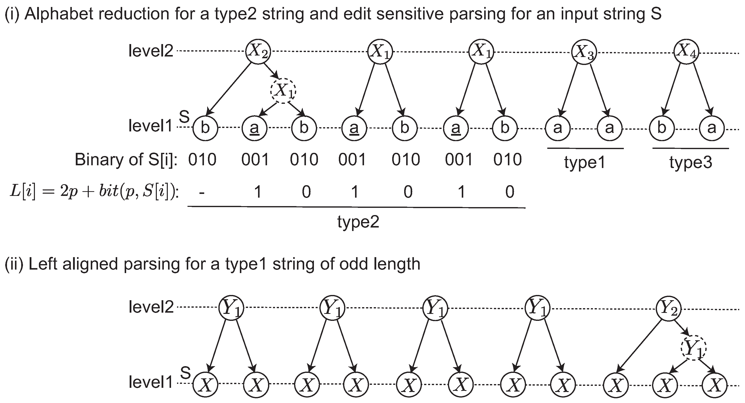
We focus on how to determine the partition S = s 1 s 2 s . A string of the form a r with a Σ V and r 2 is called a repetition. First, S is uniquely partitioned into the form w 1 x 1 w 2 x 2 w k x k w k + 1 by its maximal repetitions, where each x i is a maximal repetition of a symbol in Σ V , and each w i ( Σ V ) * contains no repetition. Then, each x i is called type1, each w i of length at least 2 lg * | S | is type2, and any remaining w i is type3. If | w i | = 1 , this symbol is attached to x i 1 or x i with preference x i 1 when both cases are possible. Thus, if | S | > 2 , each x i and w i is longer than or equal to two. One of the substrings is referred to as S i .
Next, ESP-comp parses each S i depending on the type. For type1 and type3 substrings, the algorithm performs the left aligned parsing as follows. If | S i | is even, the algorithm builds 2-tree from S i [ 2 j 1 , 2 j ] for each j { 1 , 2 , , | S i | / 2 } ; otherwise, the algorithm builds a 2-tree from S i [ 2 j 1 , 2 j ] for each j { 1 , 2 , , ( | S i | 3 ) / 2 } and builds a 2-2-tree from the last trigram S i [ | S i | 2 , | S i | ] . For type2 S i , the algorithm further partitions it into short substrings of length two or three by alphabet reduction [8].
Alphabet reduction: Given a type2 string S, consider S [ i ] and S [ i 1 ] as binary integers. Let p be the position of the least significant bit, in which S [ i ] S [ i 1 ] , and let b i t ( p , S [ i ] ) be the bit of S [ i ] at the p-th position. Then, L [ i ] = 2 p + b i t ( p , S [ i ] ) is defined for any i 2 . Because S is repetition-free (i.e., type2), the label string L ( S ) = L [ 2 ] L [ 3 ] L [ | S | ] is also type2. If the number of different symbols in S is n (denoted by [ S ] ), then [ L ( S ) ] = O ( lg n ) . For the L ( S ) , the next label string is iteratively computed until the final L * ( S ) satisfying [ L * ( S ) ] lg * | S | is obtained. S [ i ] is called the landmark if L [ i ] > max { L [ i 1 ] , L [ i + 1 ] } .
The alphabet reduction transforms S into L * ( S ) such that any substring of L * ( S ) of length at least 2 lg * | S | contains at least one landmark because L * ( S ) is also type2. Using this characteristic, the algorithm ESP-comp determines the bigrams S [ i , i + 1 ] to be replaced for any landmark S [ i ] , where any two landmarks are not adjacent, and then the replacement is deterministic. After replacing all landmarks, any remaining maximal substring s is replaced by the left aligned parsing, where if | s | = 1, it is attached to its left or right block.
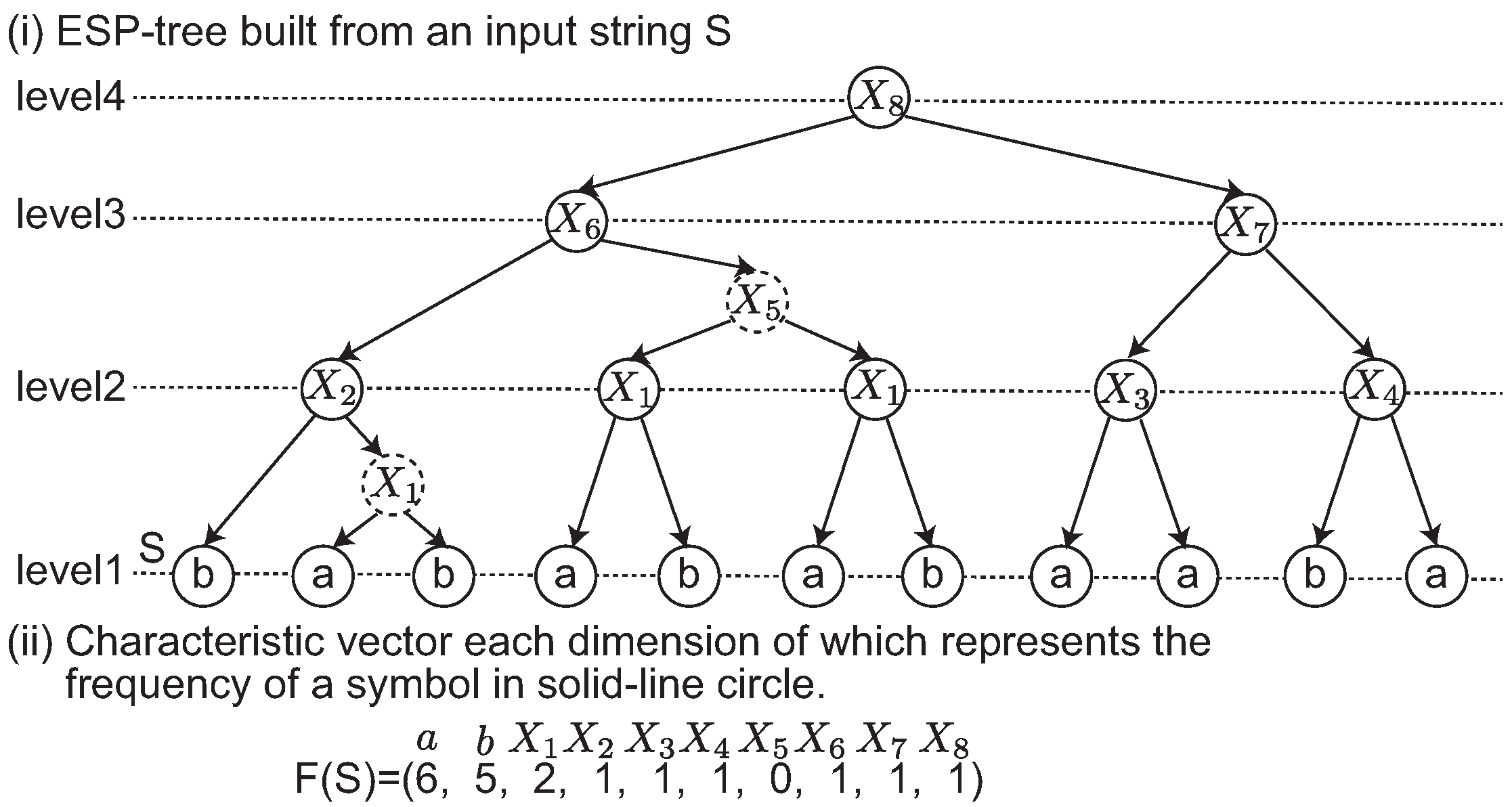
We give an example of the edit sensitive parsing of an input string in Figure 1-(i) and (ii). The input string S is divided into three maximal substrings depending on the types. The label string L is computed for the type2 string. Originally, L is iteratively computed until [ L ] lg * | S | . This case shows that a single iteration satisfies this condition. After the alphabet reduction, three landmarks S [ i ] are found, and then each S [ i , i + 1 ] is parsed. Any other remaining substrings including type1 and type3 are parsed by the left aligned parsing shown in Figure 1-(ii). In this example, a dashed node denotes that it is an intermediate node in a 2-2-tree. Originally, an ESP tree is a ternary tree in which each node has at most three children. The intermediate node is introduced to represent ESP tree as a binary tree.
As shown in [
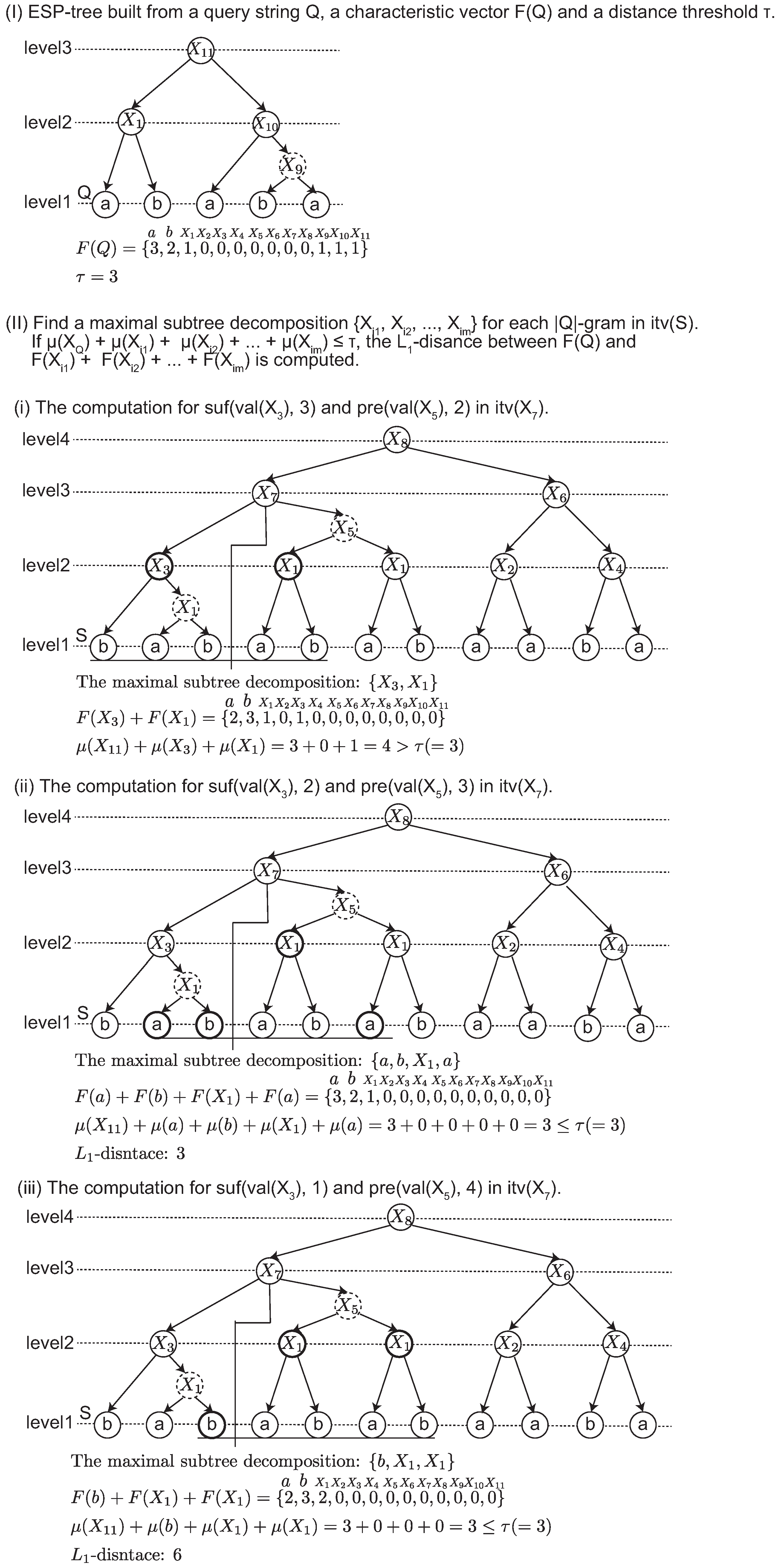
8], the alphabet reduction approximates the minimum CFG as follows. Let S be a type2 string containing a substring α at least twice. When α is sufficiently long (e.g., | α | 2 lg * | S | ), there is a partition α = α 1 α 2 such that | α 1 | = O ( lg * | S | ) and each landmark of α 2 within α is decided by only α 1 . This means the long prefix α 2 of α is replaced by the same variables, independent of the occurrence of α.
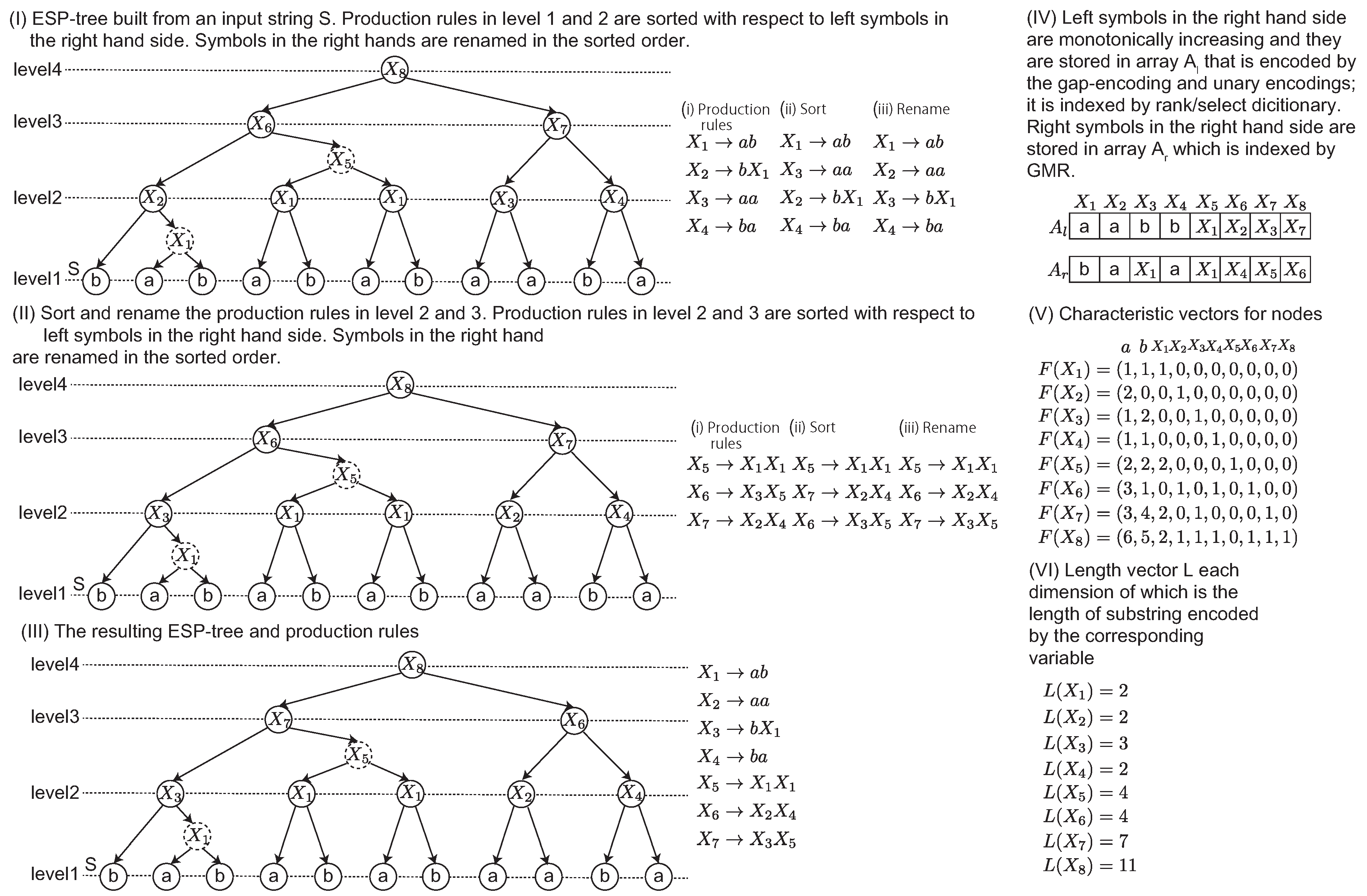
ESP-comp generates a new shorter string S of length from | S | / 3 to | S | / 2 , and it parses S iteratively. Given a string S, ESP builds the ESP-tree of height O ( lg | S | ) in O ( | S | lg * | S | ) time and in O ( | Σ V | lg | Σ V | ) space. The approximation ratio of the smallest grammar by ESP is O ( lg * | S | lg | S | ) [10].

4.2. Approximate Computations of EDM from ESP-Trees

ESP-trees enable us to approximately compute EDM for two strings. After constructing ESP-trees for two strings, their characteristic vectors are defined as follows. Let T ( S ) be the ESP-tree for string S. We define that an integer vector F ( S ) to be the characteristic vector if F ( S ) ( X ) represents the number of times the variable X appears in T ( S ) as the root of a 2-tree. For a string S, T ( S ) and its characteristic vector are illustrated in Figure 2. The EDM between two strings S and Q can be approximated by L 1 -distance between two characteristic vectors F ( S ) and F ( Q ) as follows:
F ( S ) F ( Q ) 1 = e V ( S ) V ( Q ) | F ( S ) ( e ) F ( Q ) ( e ) |
Cormode and Muthukrishnan showed the upper and lower bounds on the L 1 -distance between characteristic vectors for the exact EDM.
Theorem 1 
(Upper and lower bounds of the approximated EDM [8]) . For N = max ( | S | , | Q | ) ,
d ( S , Q ) 2 F ( S ) F ( Q ) 1 = O ( lg N lg * N ) d ( S , Q )

5. Index Structure for ESP-Trees

5.1. Efficient Encoding Scheme

siEDM encodes an ESP-tree built from a string for fast query searches. This encoding scheme sorts the production rules in an ESP-tree such that the left symbols on the right hand side of the production rules are in monotonically increasing order, which enables encoding of these production rules efficiently and supporting fast operations for ESP-trees. The encoding scheme is performed from the first and second levels to the top level (i.e., root) in an ESP-tree.
First, the set of production rules at the first and second levels in the ESP-tree is sorted in increasing order of the left symbols on the right hand of the production rules, i.e., X l ( i ) in the form of X i X l ( i ) X r ( i ) , which results in a sorted sequence of these production rules. The variables in the left hand side in the sorted production rules are renamed in the sorted order, generating a set of new production rules that is assigned to the corresponding nodes in the ESP-tree. The same scheme is applied to the next level of the ESP-tree, which iterates until it reaches the root node.
Figure 3 shows an example of the encoding scheme for the ESP-tree built from an input string S = b a b a b a b a a b a . At the first and second levels in the ESP-tree, the set of production rules, { X 1 a b , X 2 b X 1 , X 3 a a , X 4 b a } , is sorted in the lexicographic order of the left symbols on right hand sides of production rules, which results in the sequence of production rules, ( X 1 a b , X 3 a a , X 2 b X 1 , X 4 b a ) . The variables on the right hand side of the production rules are renamed in the sorted order, resulting in the new sequence ( X 1 a b , X 2 a a , X 3 b X 1 , X 4 b a ) , whose production rules are assigned to the corresponding nodes in the ESP-tree. This scheme is repeated until it reaches level 4.
Using the above encoding scheme, we obtain a monotonically increasing sequence of left symbols on the right hand side of the production rules, i.e., X l ( i ) in the form of X i X l ( i ) X r ( i ) . Let A l be the increasing sequence; A l can be efficiently encoded into a bit string by using the gap-encoding and the unary coding. For example, the gap-encoding represents the sequence ( 1 , 1 , 3 , 5 , 8 ) by ( 1 , 0 , 2 , 2 , 3 ) , and it is further transformed to the bit string 0 1 10 0 10 2 10 2 10 3 1 = 0110010010001 by unary coding. Generally, for a sequence ( x 1 , x 2 , , x n ) , its unary code U represents x i by rank 0 ( U , select 1 ( U , i ) ) . Because the number of 0s and the number of 1s is n + σ and n, respectively, the size of U is 2 n + σ bits. The bit string is indexed by the rank/select dictionary.
Let A r be the sequence consisting of the right symbols on the right hand side of the production rules, i.e., X r ( i ) in the form of X i X l ( i ) X r ( i ) . A r is represented using ( n + σ ) lg ( n + σ ) bits. A r is indexed by GMR [21].
The space for storing A l and A r is ( n + σ ) lg ( n + σ ) + 2 n + σ + o ( ( n + σ ) lg ( n + σ ) ) bits in total. A l and A r enable us to simulate fast queries on encoded ESP-trees, which is presented in the next subsection.

5.2. Query Processing on Tree

The encoded ESP-trees support four tree operations, LeftChild , RightChild , LeftParents and RightParents , which are used in our search algorithm. LeftChild ( X k ) returns the left child X l ( k ) of X k and can be implemented on bit string A l in O ( 1 ) time as m = select 1 ( A l , X k ) and LeftChild ( X k ) = m X k . RightChild ( X k ) returns the right child X r ( k ) of X k and can be implemented on array A r in O ( lg lg ( n + σ ) ) time as X j = access ( A r , X k ) .
LeftParents ( X k ) and RightParents ( X k ) return sets of parents of X k as left and right children, respectively, i.e., LeftParents ( X k ) = { X i V : X i X k X j , X j ( Σ V ) } and RightParents ( X k ) = { X i V : X i X j X k , X j ( Σ V ) } .
Because A l is a monotonic sequence, any X k appears consecutively in A l . Using the unary encoding of A l , LeftParents ( X k ) is computed by { p + i : p = select 1 ( A l , X k ) , rank 0 ( A l , p + i ) = rank 0 ( A l , p ) } in O ( | LeftParents ( X k ) | ) time. RightParents ( X k ) can be computed by repeatedly applying select operations for X k on A r until no more X k appear, i.e., select X k ( A r , p ) for 1 p n . Thus, RightParents ( X k ) for X k V can be computed in O ( | RightParents ( X k ) | ) time.

5.3. Other Data Structures

As a supplemental data structure, siEDM computes the node characteristic vector, denoted by F ( X i ) , for each variable X i : the characteristic vector consisting of the frequency of any variable derived from X i . The space for storing all node characteristic vectors of n variables is at most n 2 lg | S | bits. Figure 3-(V) shows an example of the node characteristic vectors for ESP-tree in Figure 3-(III). In addition, let V ( X i ) be a set of X i and variables appearing in all the descendant nodes under X i , i.e., V ( X i ) = { e ( V Σ ) : F ( X i ) ( e ) 0 } . Practically, F ( X i ) is represented by a sequence of a pair of X j V ( X i ) and F ( X i ) ( X j ) . Additionally, because F ( X i ) = F ( LeftChild ( X i ) ) + F ( RightChild ( X i ) ) + ( X i , 1 ) ( + ( X i , 1 ) represents adding 1 to dimension X i ), the characteristic vectors can be stored per level 2 of the ESP-tree. The data structure is represented by a bit array F B indexed by a rank/select dictionary and the characteristic vectors reduced per level 2 of ESP-tree. F B is set to 1 for i-th bit if F ( X i ) is stored, otherwise it is 0. Then, F ( X i ) can be computed by rank 1 ( F B , i ) -th characteristic vector if the i-th bit of F B is 1; otherwise, F ( LeftChild ( X i ) ) + F ( RightChild ( X i ) ) + ( X i , 1 ) .
Another data structure that siEDM uses is a non-negative integer vector named length vector, each dimension of which is the length of the substring derived from the corresponding variable (See Figure 3-(VI)). The space for storing length vectors of n variables is n lg | S | bits.
From the above argument, the space of the siEDM’s index structure for n variables is n ( n + 1 ) lg | S | + ( n + σ ) lg ( n + σ ) + 2 n + σ + o ( ( n + σ ) lg ( n + σ ) ) bits in total.

6. Search Algorithm

6.1. Baseline Algorithm

Given a T ( S ) , the maximal subtree decomposition of S [ i , j ] is a sequence ( X 1 , X 2 , , X m ) of variable in T ( S ) defined recursively as follows. X 1 is the variable of the root of the maximal subtree satisfying that S [ i ] is its leftmost leaf and | v a l ( X 1 ) | j i . If v a l ( X 1 ) = S [ i , j ] , then ( X 1 ) is the maximal subtree decomposition of S [ i , j ] . Otherwise, let X 1 , X 2 , , X m be already determined and | v a l ( X 1 ) v a l ( X 2 ) v a l ( X m ) | = k < j i . Then, let X m + 1 be the variable of the root of the maximal subtree satisfying that S [ i + k + 1 ] is its leftmost leaf and | v a l ( X m + 1 ) | j i k . Repeating this process until v a l ( X 1 ) v a l ( X 2 ) v a l ( X m ) = S [ i , j ] , the maximal subtree decomposition is determined.
Based on the maximal subtree decomposition, we explain the outline of the baseline algorithm, called online ESP [17], for computing an approximation of EDM between two strings. T ( S ) is constructed beforehand. Given a pattern Q, the online ESP computes T ( Q ) , and for each substring S [ i , j ] of length | Q | , it computes the approximate EDM as follows. It computes the maximal subtree decomposition ( X 1 , X 2 , , X m ) of S [ i , j ] . Then, the distance F ( Q ) F ( S [ i , j ] ) 1 is approximated by F ( Q ) k = 1 m F ( X k ) 1 because ESP-tree is balanced and then F ( S [ i , j ] ) k = 1 m F ( X k ) 1 = O ( lg m ) . This baseline algorithm is, however, required to compute the characteristic vector of S [ i , j ] at each position i. Next, we improve the time and space of the online ESP by finding those | Q | -grams for each variable X in V ( S ) instead of each position i.

6.2. Improvement

The siEDM approximately solves Problem 1 with the same guarantees presented in Theorem 1. Let X i V ( S ) such that | val ( X i ) | > | Q | . There are | Q | -grams formed by the string suf ( val ( X l ( i ) ) , | Q | k ) pre ( val ( X r ( i ) ) , k ) with k = 1 , 2 , , ( | Q | 1 ) . Then, the variable X i is said to stab the | Q | -grams. The set of the | Q | -grams stabbed by X i is denoted by itv ( X i ) . Let itv ( S ) be the set of itv ( X i ) for all X i appearing in T ( S ) . An important fact is that itv ( S ) includes any | Q | -gram in S. Using this characteristic, we can reduce the search space .
If a | Q | -gram R is in itv ( X i ) , there exists a maximal subtree decomposition X i 1 , X i 2 , , X i m . Then, the L 1 -distance of F ( Q ) and j = 1 m F ( X i j ) guarantees the same upper bounds in the original ESP as follows.
Theorem 2. 
Let R itv ( X i ) be a | Q | -gram on S and X i 1 , X i 2 , , X i m be its maximal subtree decomposition in the tree T ( X i ) . Then, it holds that
F ( Q ) j = 1 m F ( X i j ) 1 = O ( lg | Q | lg * | S | ) d ( Q , R )
Proof. 
By Theorem 1, F ( Q ) F ( R ) 1 = O ( lg | Q | lg * | S | ) d ( Q , R ) . On the other hand, for an occurrence of R in S, let T ( X i ) be the smallest subtree in T ( S ) containing the occurrence of R, i.e., R itv ( X i ) . For T ( R ) and T ( X i ) , let s ( R ) and s ( X i ) be the sequences of the level 2 symbols in T ( R ) and T ( X i ) , respectively. By the definition of the ESP, it holds that s ( R ) = α β γ and s ( X i ) = α β γ for some strings satisfying | α α γ γ | = O ( lg * | S | ) | , and this is true for the remaining string β iteratively. Thus, F ( R ) F ( X i ) 1 = O ( lg | R | lg * | S | ) since the trees are balanced. Hence, by the equation
F ( Q ) j = 1 m F ( X i j ) 1 = O ( lg | Q | lg * | S | ) d ( Q , R ) + O ( lg | Q | lg * | S | ) = O ( lg | Q | lg * | S | ) d ( Q , R )
we obtain the approximation ratio. ☐
To further enhance the search efficiency, we present a lower bound of the L 1 -distance between characteristic vectors, which can be used for reducing the search space.
Theorem 3 
(A lower bound μ). For any X i V ( S ) V ( Q ) , the inequality F ( S ) F ( Q ) 1 μ ( X i ) holds where
μ ( X i ) = e V ( S ) V ( Q ) F ( X i ) ( e )
Proof. 
The L 1 distance between F ( S ) and F ( Q ) is divided into four classes of terms: (i) both members in F ( S ) and F ( Q ) are non-zero, (ii) both members in F ( S ) and F ( Q ) are zero, (iii) the members in F ( S ) and F ( Q ) are zero and non-zero, (iv) the members in F ( S ) and F ( Q ) are non-zero and zero, respectively. Terms consisting of class (iii) and (iv) can be written as e V ( S ) V ( Q ) F ( S ) ( e ) , which is a lower bound of the L 1 -distance. Thus, F ( S ) F ( Q ) 1 e V ( S ) V ( Q ) F ( S ) ( e ) . ☐
Theorem 4 
(Monotonicity of μ). If a variable X i derives X k , the inequality μ ( X i ) μ ( X k ) holds.
Proof. 
Every entry in F ( X k ) is less than or equal to the corresponding entry in F ( X i ) . Thus, the inequality holds. ☐

6.3. Candidate Finding

By Theorems 2, 3 and 4, the task of the algorithm is reduced to finding a maximal subtree decomposition ( X i 1 , X i 2 , , X i m ) within X i . Given a threshold τ 0 , for each | Q | -gram in itv ( S ) , the algorithm finds the candidate: the maximal subtree decomposition ( X i 1 , X i 2 , , X i m ) satisfying μ ( X i 1 ) + μ ( X i 2 ) + + μ ( X i m ) τ .
For an X i and an occurrence of some | Q | -gram in itv ( X i ) , the | Q | -gram is formed by the expression suf ( val ( X l ( i ) ) , | Q | k ) pre ( val ( X r ( i ) ) , k ) for a k ( 1 k | Q | 1 ) . The algorithm computes the maximal subtree decompositions ( x 1 , x 2 , , x p ) covering suf ( val ( X l ( i ) ) , | Q | k ) and ( y 1 , y 2 , , y q ) covering pre ( val ( X r ( i ) ) , k ) , and outputs ( x 1 , , x p , y 1 , , y q ) covering the | Q | -gram when 1 i p μ ( x i ) + 1 i q μ ( y i ) τ . We illustrate the computation of candidates satisfying μ ( X i 1 ) + μ ( X i 2 ) + + μ ( X i m ) τ in Figure 4 and show the pseudo-code in Algorithm 1.
Applying all variables to Algorithm 1 enables us to find the candidates covering all solutions. There are no possibilities for missing any | Q | -grams in itv ( S ) such that the L 1 -distances between their characteristic vectors and F ( Q ) are at most τ, i.e., false negatives. The set may include a false positive, i.e., the solution set encodes a | Q | -gram such that the L 1 -distance between its characteristic vector and F ( Q ) is more than τ. However, false positives are efficiently removed by computing the L 1 -distance F ( Q ) j = 1 m F ( X i j ) 1 as a post-processing.
Theorem 5. 
The computation time of FindCandidates is O ( n | Q | lg lg ( n + σ ) ( lg | S | + lg | Q | ) ) .
Proof. 
Because the height of the ESP-tree is O ( lg | S | ) , for each variable X, the number of visited nodes is O ( lg | Q | + lg | S | ) . The computation time of LeftChild ( X ) and RightChild ( X ) is O ( lg lg ( n + σ ) ) , and the time of FindLeft and FindRight is O ( | Q | lg lg ( n + σ ) ( lg | S | + lg | Q | ) ) . Thus, for n iterations of the functions, the total computation time is O ( n | Q | lg lg ( n + σ ) ( lg | S | + lg | Q | ) ) . ☐
Algorithm 1 to output the candidate R V ( S ) for X V ( S ) , a query pattern Q and a distance threshold τ.
1:
function FindCandidates(X,Q,τ)
2:
    for j = 1 , 2 , , | Q | do
3:
         R ϕ                              ▹ Initialize solution set 
4:
         q 1 FindLeft( LeftChild ( X ) , | Q | j , 0 , R )                ▹ for left child 
5:
         q 2 FindRight( RightChild ( X ) , j , 0 , R )                 ▹ for right child 
6:
        if q 1 = 0 and q 2 = 0 then 
7:
           Output R 
8:
function FindLeft( X , q , d , R
9:
    if d > τ then 
10:
        return  
11:
    else if q = 0 then 
12:
        return 0 
13:
    else if X Σ then 
14:
         d d + 1  if X V ( Q )  
15:
         R R { X }  
16:
        return q 1  
17:
    else if | val ( X ) | q then 
18:
         d d + μ ( X )  
19:
         R R { X }  
20:
        return q | val ( X ) |  
21:
     q FindLeft( RightChild ( X ) , q , d , R
22:
    if q 0 then 
23:
        return FindLeft ( LeftChild ( X ) , q , d , R )  
24:
function FindRight( X , q , d , R
25:
    if d > τ then 
26:
        return  
27:
    else if q = 0 then 
28:
        return 0 
29:
    else if X Σ then 
30:
         d d + 1 if X V ( Q )  
31:
         R R { X }  
32:
        return q 1  
33:
    else if | val ( X ) | q then 
34:
         d d + μ ( X )  
35:
         R R { X }  
36:
        return q | val ( X ) |  
37:
     q FindRight( LeftChild ( X ) , q , d , R
38:
    if q 0 then 
39:
        return FindRight ( RightChild ( X ) , q , d , R )  

6.4. Computing Positions

The algorithm also computes all the positions of val ( X i ) , denoted by P ( X i ) = { p { 1 , 2 , , | S | } : S [ p , p + | val ( X i ) | 1 ] = ( X i ) } . Starting from X i , the algorithm goes up to the root in the ESP-tree built from S. p is initialized to 0 at X i . If X k through the pass from X i to the root is the parent with the right child X r ( k ) on the pass, non-negative integer ( | val ( X k ) | | val ( X r ( k ) ) | ) is added to p. Otherwise, nothing is added to p. When the algorithm reaches the root, p represents a start position of val ( X i ) on S, i.e., val ( X i ) = S [ p , p + | val ( X i ) | 1 ] . To compute the set P ( X i ) , the algorithm starts from X i and goes up to the root for each parent in RightParents ( X i ) and LeftParents ( X i ) , which return sets of parents for X i . Algorithm 2 shows the pseudo-code.
Algorithm 2 to compute the set P of all occurrence of val ( X ) on S for X V ( S ) .
1:
function ComputePosition(X
2:
     P { }                    ▹ Initialize solution set 
3:
    Recursion(X, 1) 
4:
function Recursion(X,p
5:
    if X is the root node then 
6:
         P P { p }  
7:
        return
8:
    for each X p RightParents ( X ) do      ▹X is the right child of X p  
9:
        Recursion( X p , p + | val ( X p ) | | val ( X ) |
10:
    for each X p LeftParents ( X ) do       ▹X is the left child of X p  
11:
        Recursion( X p ,p
Theorem 6. 
The computation time of P ( X ) is O ( occ lg | S | ) , where occ is the number of occurrences of X in T ( S ) .
Proof. 
Using the index structures of RightParents ( X ) and LeftParents ( X ) , we can traverse the path from any node with label ( X ) to the root of T ( S ) counting the position. The length of the path is O ( lg | S | ) . ☐
Theorem 7. 
The search time is O ( n | Q | lg lg ( n + σ ) ( lg | S | + lg | Q | ) + o c c lg | S | ) using the data structure of size n ( n + 1 ) lg | S | + ( n + σ ) lg ( n + σ ) + 2 n + σ + o ( ( n + σ ) lg ( n + σ ) ) bits.
Proof. 
The time for computing T ( Q ) and F ( Q ) is t 1 = O ( | Q | lg * | S | ) . The time for finding candidates and computing F ( Q ) j = 1 m X i j 1 is t 2 = O ( n | Q | lg lg ( n + σ ) ( lg | S | + lg | Q | ) ) by Theorem 5. The time for computing positions is O ( o c c lg | S | ) by Theorem 6. Thus, the total time for a query search is t 1 + t 2 + t 3 = O ( n | Q | lg lg ( n + σ ) ( lg | S | + lg | Q | ) + o c c lg | S | ) . The size of the data structure is derived by the results in Section 5. ☐
In Theorem 7, n and o c c are incomparable because o c c > n is possible for a highly repetitive string.

7. Experiments

We evaluated the performance of siEDM on one core of a quad-core Intel Xeon Processor E5540 (2.53GHz) machine with 144GB memory. We implemented siEDM using the rank/select dictionary and GMR in libcds (https://github.com/fclaude/libcds). We used two standard benchmark datasets of einstein and cere from repetitive text collections in the pizza and chili corpus (http://pizzachili.dcc.uchile.cl/repcorpus.html), which is detailed in Table 1. As a comparison method, we used the online pattern matching for EDM called online ESP (baseline) [17] that approximates EDM between a query Q and substrings of the length of | Q | of each position of an input text. We randomly selected S [ i , j ] as the query pattern Q for each | Q | = 50 , 100 , 500 , 1000 and examined the performance.
Table 2 shows the memory consumption in the search of the siEDM and baseline. The memory consumption of siEDM was larger than the baseline for both texts because the baseline does not have characteristic vectors of each node and length vector.
Table 3 shows the size for each component of the index structure and the time for building the index structure on einstein and cere datasets. Most of the size of the index structure was consumed by the characteristic vector F. The index size of cere was much larger than that of einstein. The index sizes of cere and einstein were approximately 16 megabytes and 256 megabytes, respectively, because the number of variables generated from cere was much larger than that generated from einstein. The number of variables generated from einstein was 305 , 098 and the number of variables generated from cere was 4 , 512 , 406 . The construction times of the index structures were 118 s for einstein and 472 s for cere. The results for constructing the index structures demonstrate the applicability of siEDM to moderately large, repetitive texts.
Figure 5 shows the total search time (sec.) of siEDM and the baseline for einstein and cere in distance thresholds τ from 10 to 60. In addition, this result does not contain the case τ < 10 because siEDM found no candidate under the condition. The query length is one of { 50 , 100 , 500 , 1000 } . Because the search time of baseline is linear in | S | + | Q | , we show only the fastest case: q = | Q | = 50 . The search time of siEDM was faster than baseline in most cases.
Figure 6 shows the detailed search time in second. CF is the time for finding candidates of Q in T ( S ) , DIST is the time for computing approximated L 1 distance by characteristic vectors, and PC is the time for determining the positions of all | Q | -grams within the threshold τ.
Figure 7 shows the number of nodes T ( S ) visited by the algorithm, #TN, the number of candidate | Q | -grams computed by F i n d C a n d i d a t e s , #CAND, the number of true positives among candidate | Q | -grams, #TP, and the number of occurrences, #OCC. The most time-consuming task is the candidate finding.
By the monotonicity of characteristic vectors, pruning the search space for small distance thresholds and long query length is more efficient. Thus, it is expected that siEDM is faster for smaller distance thresholds and longer query lengths and the experimental results support this. The search time on cere is much slower than that on einstein because the number of generated production rules from cere is much larger than that from einstein, and a large number of iterations of FindCandidates is executed. In addition, the comparison of #CAND and #TP validates the efficiency of siEDM for candidate finding with the proposed pruning method.
In Figure 7, the algorithm failed to find a candidate. Such a phenomenon often appears when the required threshold τ is too small, because the ESP-tree T ( Q ) is not necessarily identical to T ( S [ i , j ] ) even if Q = S [ i , j ] . Generally, the parsing of T ( S [ i , j ] ) is affected by a suffix of S [ 1 , i 1 ] and a prefix of S [ j + 1 , | S | ] of length at most lg * | S | .
As shown in Table 3 and Figure 5, the search time of siEDM depends on the size of encoded ESP-tree for the input. Finally, we confirm this feature by an additional experiment for other repetitive texts. Table 4, Table 5 and Table 6 are the description of several datasets from the pizza & chili corpus. Figure 8 shows the search time of siEDM and baseline. This result supports our claim that siEDM is suitable for computing EDM of repetitive texts.

8. Conclusions

We have proposed siEDM, an efficient string index for computing approximate searching based on EDM. Experimental results demonstrated the applicability of siEDM to real-world repetitive text collections as well as a longer pattern search. Future work will make the search algorithm in siEDM faster, which would be beneficial for users performing query searches for EDM.

Acknowledgments

This work was supported by Grant-in-Aid for JSPS Fellows, JSPS KAKENHI (24700140,26280088) and the JST PRESTO program. The authors thank the anonymous reviewers for their valuable feedback. The authors also thank T. Ohnishi and S. Fukunaga for their assistance.

Author Contributions

All the authors contributed equally to this work.

Conflicts of Interest

The authors declare no conflict of interest.

References

  1. Takabatake, Y.; Tabei, Y.; Sakamoto, H. Improved ESP-index: A Practical Self-Index for Highly Repetitive Texts. In Proceedings of the 13th International Symposium on Experimental Algorithms (SEA), Copenhargen, Denmark, 29 June–1 July 2014; pp. 338–350.
  2. Claude, F.; Navarro, G. Self-indexed grammar-based compression. Fundam. Inform. 2011, 111, 313–337. [Google Scholar]
  3. Gagie, T.; Gawrychowski, P.; Kärkkäinen, J.; Nekrich, Y.; Puglisi, S.J. LZ77-Based Self-Indexing with Faster Pattern Matching. In Proceedings of the 11th Latin American Theretical Informatics Symposium (LATIN), Montevideo, Uruguay, 31 March–4 April 2014; pp. 731–742.
  4. Gagie, T.; Puglisi, S.J. Searching and Indexing Genomic Databases via Kernelization. Front. Bioeng. Biotechnol. 2015, 3, 12. [Google Scholar] [CrossRef] [PubMed]
  5. Durbin, R.; Eddy, S.; Krogh, A.; Mitchison, G. Biological Sequence Analysis: Probabilistic Models of Proteins and Nucleic Acids; Cambridge University Press: Cambridge, UK, 1998. [Google Scholar]
  6. Crochemore, M.; Rytter, W. Text Algorithms; Oxford University Press: Oxford, UK, 1994. [Google Scholar]
  7. Levenshtein, V.I. Binary codes capable of correcting deletions, insertions and reversals. Sov. phys. dokl. 1996, 10, 707–710. [Google Scholar]
  8. Cormode, G.; Muthukrishnan, S. The String Edit Distance Matching Problem with Moves. ACM Trans. Algor. 2007, 3, 1–19. [Google Scholar] [CrossRef]
  9. Shapira, D.; Storer, J.A. Edit distance with move operations. J. Discret. Algorithms 2007, 5, 380–392. [Google Scholar] [CrossRef]
  10. Sakamoto, H.; Maruyama, S.; Kida, T.; Shimozono, S. A Space-Saving Approximation Algorithm for Grammar-Based Compression. IEICE Trans. Inf. Syst. 2009, 92-D, 158–165. [Google Scholar] [CrossRef]
  11. Maruyama, S.; Sakamoto, H.; Takeda, M. An Online Algorithm for Lightweight Grammar-Based Compression. Algorithms 2012, 5, 213–235. [Google Scholar] [CrossRef]
  12. Maruyama, S.; Tabei, Y.; Sakamoto, H.; Sadakane, K. Fully-online grammar compression. In Proceedings of the 20th International Symposium on String Processing and Information Retrieval Symposium (SPIRE), Jerusalem, Israel, 7–9 October 2013; pp. 218–229.
  13. Maruyama, S.; Tabei, Y. Fully-online grammar compression in constant space. In Proceedings of the Data Compression Conference (DCC), Snowbird, UT, USA, 26–28 March 2014; pp. 218–229.
  14. Maruyama, S.; Nakahara, M.; Kishiue, N.; Sakamoto, H. ESP-Index: A Compressed Index Based on Edit-Sensitive Parsing. J. Discrete Alogrithms 2013, 18, 100–112. [Google Scholar] [CrossRef]
  15. Takabatake, Y.; Tabei, Y.; Sakamoto, H. Online Self-Indexed Grammar Compression. In Proceedings of the 22nd International Symposium on String Processing and Information Retrieval (SPIRE), London, UK, 1–4 September 2015; pp. 258–269.
  16. Nakahara, M.; Maruyama, S.; Kuboyama, T.; Sakamoto, H. Scalable Detection of Frequent Substrings by Grammar-Based Compression. IEICE Trans. Inf. Syst. 2013, 96-D, 457–464. [Google Scholar] [CrossRef]
  17. Takabatake, Y.; Tabei, Y.; Sakamoto, H. Online Pattern Matching for String Edit Distance with Moves. In Proceedings of the 21st International Symposium on String Processing and Information Retrieva (SPIRE), Ouro Preto, Brazil, 20–22 October 2014; pp. 203–214.
  18. Karpinski, M.; Rytter, W.; Shinohara, A. An efficient pattern-matching algorithm for strings with short descriptions. Nord. J. Comput. 1997, 4, 172–186. [Google Scholar]
  19. Jacobson, G. Space-Efficient Static Trees and Graphs. In Proceedings of the 30th Annual Symposium on Foundations of Computer Science (FOCS), Research Triangle Park, NC, USA, 30 October–1 November 1989; pp. 549–554.
  20. Raman, R.; Raman, V.; Rao, S.S. Succinct indexable dictionaries with applications to encoding k-ary trees, prefix sums and multisets. ACM Trans. Algor. 2007, 3. [Google Scholar] [CrossRef]
  21. Golynski, A.; Munro, J.I.; Rao, S.S. Rank/select operations on large alphabets: A tool for text indexing. In Proceedings of the 17th Annual ACM-SIAM Symposium on Discrete Algorithms (SODA), Miami, FL, USA, 22–26 January 2006; pp. 368–373.
Figure 1. The edit sensitive parsing. In (i), an underlined S [ i ] means a landmark, and p 0 . In (i) and (ii), a dashed node is corresponding to the intermediate node in a 2-2-tree.
Algorithms 09 00026 g001
Figure 2. Illustration of edit sensitive parsing (ESP)-tree and characteristic vector.
Algorithms 09 00026 g002
Figure 3. Illustration of encoding scheme.
Algorithms 09 00026 g003
Figure 4. Illustration of candidate finding and L 1 -distance computation.
Algorithms 09 00026 g004
Figure 5. Comparison of the search time for einstein (left) and cere (right).
Algorithms 09 00026 g005
Figure 6. Details of search time for different | Q | and τ: time for candidate findings, CF, time for L 1 -distance computations, DIST, and time for position computations, PC. (a) and (b) correspond to CF, (c) and (d) correspond to DIST, and (e) and (f) correspond to PC of einstein and cere, respectively.
Algorithms 09 00026 g006
Figure 7. Statistical information of the query search: the number of traversed nodes, #TN, the number of candidate | Q | -grams, #CAND, the number of true positives, #TP, the number of occurrences, #OCC. (a) and (b) correspond to #TN, (c) and (d) correspond to #CAND, (e) and (f) correspond to #TP, and (g) and (h) correspond to #TP of einstein and cere, respectively.
Algorithms 09 00026 g007
Figure 8. Search time (sec.) for repetitive texts: E. coli (left) and influenza (right).
Algorithms 09 00026 g008
Table 1. Summary of datasets.
DatasetLength | Σ | Size (MB)
einstein 467 , 626 , 544 139446
cere 461 , 286 , 644 5440
Table 2. Comparison of the memory consumption for the query search.
DatasetEinsteinCere
siEDM (MB) 17.12 254.75
baseline (MB) 6.98 10.95
Table 3. Comparison of the index size and construction time.
DatasetEinsteinCere
Encoded ESP-tree (MB) 1.18 19.92
Index SizeCharacteristic vector F (MB) 15.35 227.34
Length vector L (MB) 0.59 7.49
Construction time (sec) 117.65 472.21
Table 4. Summary of additional datasets.
DatasetLength | Σ | Size (MB)
influenza15480855515 147.64
Escherichia_Coli11268951515 107.47
Table 5. Comparison of the memory consumption for the query search.
DatasetInfluenzaEscherichia_Coli
siEDM (MB) 164.87 262.01
baseline (MB) 53.01 100.81
Table 6. Comparison of the index size and construction time for additional datasets.
DatasetInfluenzaEscherichia_Coli
Encoded ESP-tree (MB) 9.92 20.21
Index SizeCharacteristic vector F (MB) 150.87 234.91
Length vector L (MB) 4.08 6.88
Construction time (sec) 290.33 420.43

