
Predicting Decompensation Risk in Intensive Care Unit Patients Using Machine Learning


1
Data Science Research Centre, Liverpool John Moores University, Liverpool L3 3AF, UK
2
Liverpool Centre for Cardiovascular Science, University of Liverpool, Liverpool John Moores University and Liverpool Heart & Chest Hospital, Liverpool L3 3AF, UK
*
Author to whom correspondence should be addressed.
Algorithms 2024, 17(1), 6; https://doi.org/10.3390/a17010006
Submission received: 2 November 2023
/
Revised: 18 December 2023
/
Accepted: 21 December 2023
/
Published: 22 December 2023
(This article belongs to the Special Issue Machine Learning Algorithms and Methods for Predictive Analytics)
Abstract
:Patients in Intensive Care Units (ICU) face the threat of decompensation, a rapid decline in health associated with a high risk of death. This study focuses on creating and evaluating machine learning (ML) models to predict decompensation risk in ICU patients. It proposes a novel approach using patient vitals and clinical data within a specified timeframe to forecast decompensation risk sequences. The study implemented and assessed long short-term memory (LSTM) and hybrid convolutional neural network (CNN)-LSTM architectures, along with traditional ML algorithms as baselines. Additionally, it introduced a novel decompensation score based on the predicted risk, validated through principal component analysis (PCA) and k-means analysis for risk stratification. The results showed that, with PPV = 0.80, NPV = 0.96 and AUC-ROC = 0.90, CNN-LSTM had the best performance when predicting decompensation risk sequences. The decompensation score’s effectiveness was also confirmed (PPV = 0.83 and NPV = 0.96). SHAP plots were generated for the overall model and two risk strata, illustrating variations in feature importance and their associations with the predicted risk. Notably, this study represents the first attempt to predict a sequence of decompensation risks rather than single events, a critical advancement given the challenge of early decompensation detection. Predicting a sequence facilitates early detection of increased decompensation risk and pace, potentially leading to saving more lives.
1. Introduction
Intensive Care Units (ICUs) are specialist hospital wards that provide treatment and monitoring to critically ill patients, where prompt identification of deteriorating patient health is paramount. Decompensation, marked by rapid health decline, poses severe risks and underscores the need for timely detection. Conventional methods often fall short, prompting exploration into advanced predictive techniques [1].
Predicting ICU decompensation events has been explored in several ways. For instance, Kia et al. [2] used Support Vector Machines (SVM), Random Forest (RF), and Logistic Regression (LR) to forecast decompensation events within ICUs. Their developed models were compared against the standard Modified Early Warning Score (MEWS). With an Area Under the Receiver Operating Characteristic Curve (AUC) of 0.85, they found RF presented the best overall performance. An alternative approach using Gradient Boosting Machines (GBMs) was proposed by Ruiz et al. [3]. Their approach showed an AUC of 0.92 at 4 h, and 0.82 at 8 h before the decompensation event occurred.
Deep Learning (DL) algorithms have also been used for decompensation modelling in ICU. Thorsen-Meyer et al. [4] trained a Long Short-Term Memory (LSTM) neural network on static data and physiological time-series data sourced from the Danish National Patient Registry, obtaining equivalent performance results. The use of DL is attractive as it can efficiently capture dynamic fluctuations in vitals and other clinical characteristics, thereby enhancing model performance.
One major criticism of DL models has traditionally been their difficulty in explaining predictions, which is an essential requirement in medical research and healthcare applications. In recent years, there has been an increased effort to develop Explainable AI (xAI) algorithms specifically for DL models, particularly in health research. Ho et al. [5] combined Learned Binary Masks (LBM) with Kernel Shapley Additive exPlanations (KernelSHAP) values to explain Recurrent Neural Network (RNN) mortality risk prediction models in critically ill children using electronic medical records (EMR). Another approach, named Windowed Feature Importance in Time (WinIT) [6], encapsulates the changing importance of a feature over time, providing an aggregated understanding of its significance by cumulatively assessing feature importance over a window of preceding time steps.
This study aims to develop and assess machine learning (ML) models for predicting the risk of decompensation events in patients admitted to ICUs. Specifically, we propose a novel methodological approach that implements a sequence-to-sequence risk prediction task. It utilises a sequence of patient’s vitals and other clinical characteristics within a specified time window to forecast a decompensation risk sequence in a subsequent time window (i.e., forecast window). For this purpose, we considered two DL architectures: the many-to-many long short-term memory (LSTM) [7] and the hybrid convolutional neural network and LSTM (CNN-LSTM) [8].
Our approach reflects the dynamic nature of patient decompensation, rather than treating it as a single event. We used the predicted sequence to propose a novel decompensation score. Additionally, predicting a sequence could enable earlier detection of decompensation, facilitating prompt intervention and potentially leading to improved patient outcomes.
2. Materials and Methods
2.1. Data Extraction
Data was extracted from the Medical Information Mart for Intensive Care IV (MIMIC-IV, [9]), a freely available database of de-identified electronic health records linked to patients admitted to the Beth Israel Deaconess Medical Centre in Boston, Massachusetts. We used version 2.2, released in January 2023, which comprises 299,712 patients, 431,231 hospital admissions and 73,181 ICU stays.
For this study, we extracted sequences of vitals (e.g., temperature, heart rate, and respiratory rate), lab test results (e.g., glucose, haemoglobin, and platelet count), and other clinical characteristics of the patients admitted to the hospital’s ICU (e.g., age, height, and weight). Patients < 18 years old, patient admissions with short ICU stays (<24 h), and patients with multiple ICU stays were excluded from the study. Invalid values of the variables (e.g., heart rate < 0) were marked as not available. Variables recorded with different units were harmonised, e.g., height was present in inches and centimetres (cm), and they were all converted to cm. The data used for modelling was formatted as a three-dimensional array, with dimensions representing patient admissions, time points (hours), and variables.
As common in health data, extracted data records were frequently incomplete. Records with missing age, haemoglobin, platelet count, or oxygen saturation were removed from the dataset. For the remaining variables, missing values were handled as follows: for gaps in continuous-valued time series, the last observation carried forward (LOCF) method [10] was employed, while the mode was used to impute missing values in categorical variables. Time series with all values missing in a single admission were completed in the way described in [11].
2.2. Modelling Methodology
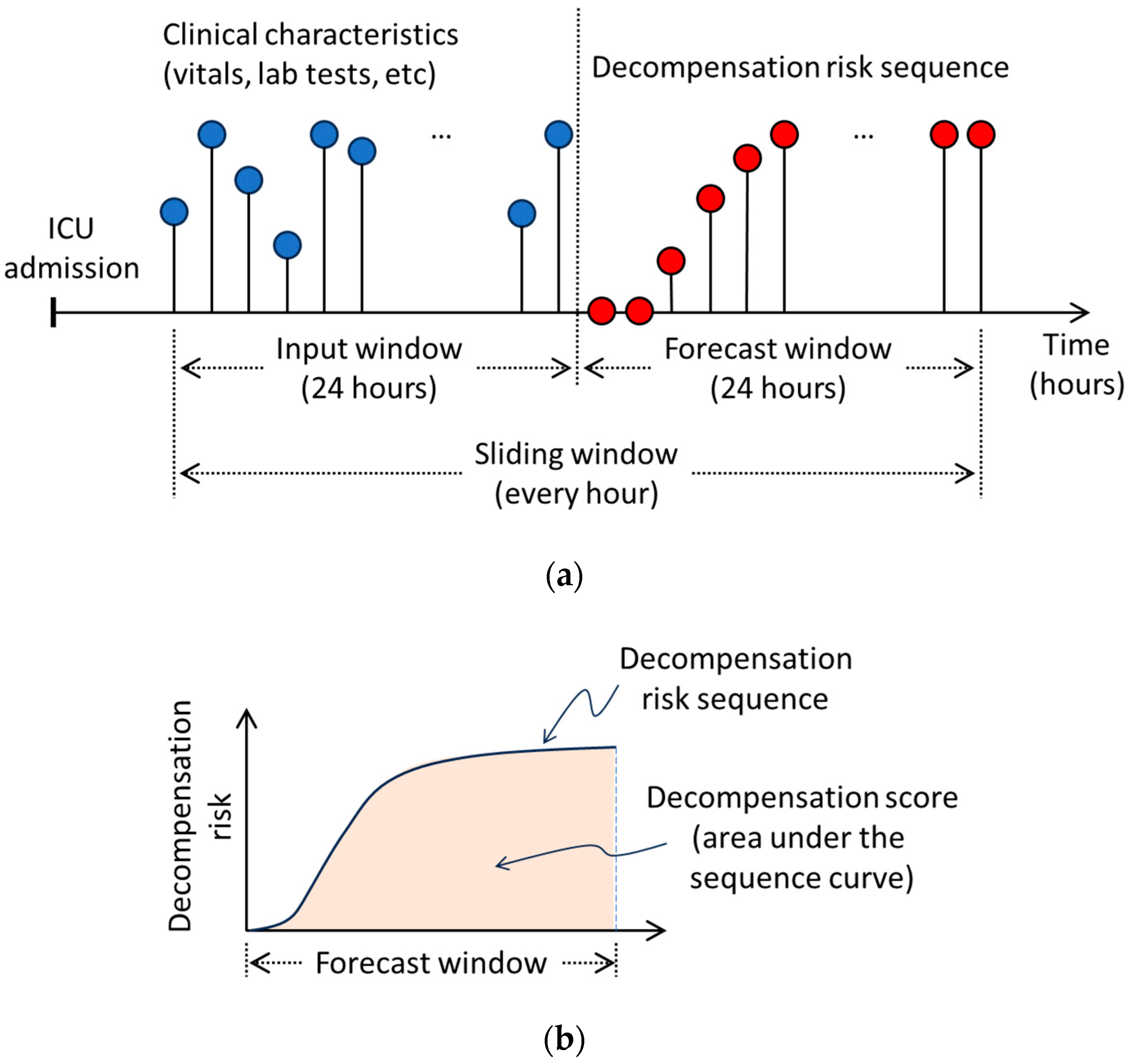
Our proposed decompensation risk prediction model implements a sequence-to-sequence approach that processes sequences of clinical characteristics within a 24-h input time window, predicting the risk of a decompensation event every hour during a 24-h forecast period. We define the decompensation event as a 2-class problem (i.e., decompensation, no-decompensation), and predicting the risk of a decompensation event as the problem of predicting the probability of such event to happen. A patient is coded as decompensating if they would be recorded as having died 24 h later. This definition accounts for the fact that a patient is at high risk of dying at any time after a decompensation event has started. This is a more conservative approach than the one used in [11]. Two DL architectures were considered in the development of the sequence-to-sequence risk prediction model: LSTM and hybrid CNN-LSTM. We propose a patient’s decompensation score, which is defined as the area under the predicted sequence of decompensation risk within the forecast window. For each patient, the decompensation score is calculated every hour after the 24-h input window, using the 24-h forecast window. This sliding window continues to move until the patient is discharged from the ICU.
In addition, we developed baseline models based on traditional ML algorithms such as LR, SVM, and RF, although their tasks were modified since they are not designed for handling time series. Therefore, instead of predicting a time series, they were implemented to predict one decompensation event within the forecast period. Therefore, the sole purpose of these baseline models is to establish the minimum performance level against which the DL algorithms should be evaluated.
Numerical variables were standardised (i.e., mean-centred and scaled by the standard deviation), whilst one-hot encoding was applied to the categorical variables. The methodological approach used in this study is illustrated in Figure 1.
2.2.1. Traditional ML Algorithms
The traditional ML algorithms LR, SVM, and RF were used as baseline models [12]. Widely used in statistics, LR estimates the log odds of the output as the linear combination of the input variables. SVM finds a hyperplane that best separates different classes in the feature space, maximising the margin between them. RF is an ensemble learning method that combines multiple decision trees to improve model performance and mitigate overfitting. These algorithms were used to perform the classification task of predicting the risk of decompensation within the 24-h forecast window. However, since they cannot directly model time-series variables, they were trained on extracted hand-crafted statistical features from the input time series, i.e., mean, median, standard deviation, average absolute deviation (AAD), minimum and maximum values, interquartile range, peaks, differences between maximum and minimum values, median absolute deviation, and the count of values above the mean for each feature.
2.2.2. DL Algorithms
DL algorithms were employed to model the risk of decompensation as a sequence-to-sequence task. We chose two DL architectures, both designed for handling time series: many-to-many LSTM and CNN-LSTM.
The Many-to-Many LSTM architecture is a type of recurrent neural network designed for sequence-to-sequence tasks [13]. It takes a sequence of input data and generates a corresponding sequence of output predictions, allowing for variable-length input and output sequences.
The CNN-LSTM architecture has two identifiable stages: a channel-wise CNN and an LSTM stage [14]. The rationale behind this architecture is that the CNN stage processes sequential data with multiple channels, generating sequential outputs for each channel, whilst the LSTM stage integrates them to predict the sequence output.
2.2.3. Model Evaluation and Hyperparameter Tuning
All models were evaluated in terms of their generalisation performance using a class-stratified randomly selected test set, which accounted for 30% of the overall data. Traditional ML models were optimised by tuning their relevant hyperparameters through 10-fold cross-validation on the remaining data. For the DL models, hyperparameter tuning was performed using a randomly selected validation subset that constituted 20% of the remaining data. Table 1 displays the considered hyperparameter values.
Model performance was measured using balanced accuracy, positive and negative predicted values (PPV and NPV), the area under the precision-recall curve (AUC-PR), the area under the receiver operating characteristic curve (AUC-ROC), and the Matthews correlation coefficient (MCC). The Youden’s J statistic [15] was used to select the optimal ROC’s cut-off point.
2.3. Decompensation Score
We propose a patient’s decompensation score, which is defined as the area under the predicted sequence of decompensation risk within the forecast window, and is formulated as follows:
where is the predicted decompensation risk, is a time point within a -hour forecast window (e.g., 24 h), and , the sequence of decompensation risks. Since the risk could take a value between 0 and 1, the proposed decompensation score could range from zero (lowest) to (highest). A patient with a low decompensation score value suggests they are less likely to decompensate within the considered forecast window. In this study we used , although the length of the forecast window could be altered if the available data allows.
To assess the proposed decompensation score, it was compared against the National Early Warning Score (NEWS, [16]). NEWS is widely used in many healthcare settings worldwide, primarily in the UK, as the standard score for detecting deterioration in acutely ill patients. NEWS values could range from 0 to 20, and it is generally recognised that a value between 0 and 5 indicates a low risk of deterioration, while values above 10 represent a high risk of deterioration.
2.4. Model Interpretation
2.4.1. Model Interpretation via SHAP Values
SHapley Additive exPlanations (SHAP) [17], a popular xAI technique that originated from game theory, was used to find associations between the input time series variables and the predicted outcome of decompensation risk. Specifically, we used the DeepExplainer variant, which is designed to work with DL algorithms [18].
Given the computational complexity, utilising the entire dataset for SHAP analysis was unfeasible. Hence, we opted to randomly select 1000 data samples (i.e., ICU admissions).
2.4.2. Understanding Patient’s Predicted Decompensation Risk Sequences
To visually explore the predicted risks of decompensation, an additional dataset was created using the predicted risks from the DL models. The new dataset comprises 24 columns, representing the 24-h forecast window. Each value in the dataset indicates the patient’s predicted probability of decompensation at a specific hour. Subsequently, principal component analysis (PCA) was performed on the derived dataset, and a score plot was generated with the first 2 principal components (PCs). The rationale behind this approach was to investigate differences between patients at high and low risk of decompensation. Therefore, a patient with high-risk values at all hours (indicating a very high risk of decompensation) should be positioned far away in the PCA scores plot from a patient who, for instance, had low predicted risk values. A k-means analysis was then applied to the projected PCA data to perform decompensation risk stratification. Each stratum (k-means cluster) was interpreted using SHAP values.
3. Results
3.1. Dataset Used in This Study
The final dataset extracted and used in this study comprises 37,042 patient admissions and 22 variables of which 19 are time-varying attributes. Table 2 shows the list of these variables, including summary statistics for each of them (median and first and third quartile for numeric variables, and prevalence for binary variables), the minimum and maximum values, the level of missing values, and the imputed values.
3.2. Model Performance
Table 3 displays model performance results measured on the test set after calculating the optimal ROC’s threshold. It can be seen that RF and CNN-LSTM yielded the best performance among the baseline ML and DL models, respectively. It is worth noting that the baseline ML and DL models are not directly comparable due to differences in the modelling tasks. The best set of hyperparameters for SVM and RF are shown in Table 4.
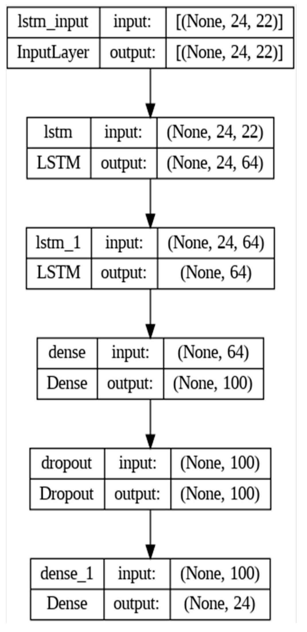
Figure 2 shows the optimised LSTM model after hyperparameter tuning. The optimal architecture consisted of two LSTM layers of 64 units each followed by a hidden dense layer of 100 and an output dense layer of 24 units, one for each hour. ReLU and sigmoid activation functions were used in the hidden and output dense layers, respectively. A dropout layer with a drop rate of 0.5 was added after the hidden dense layer.
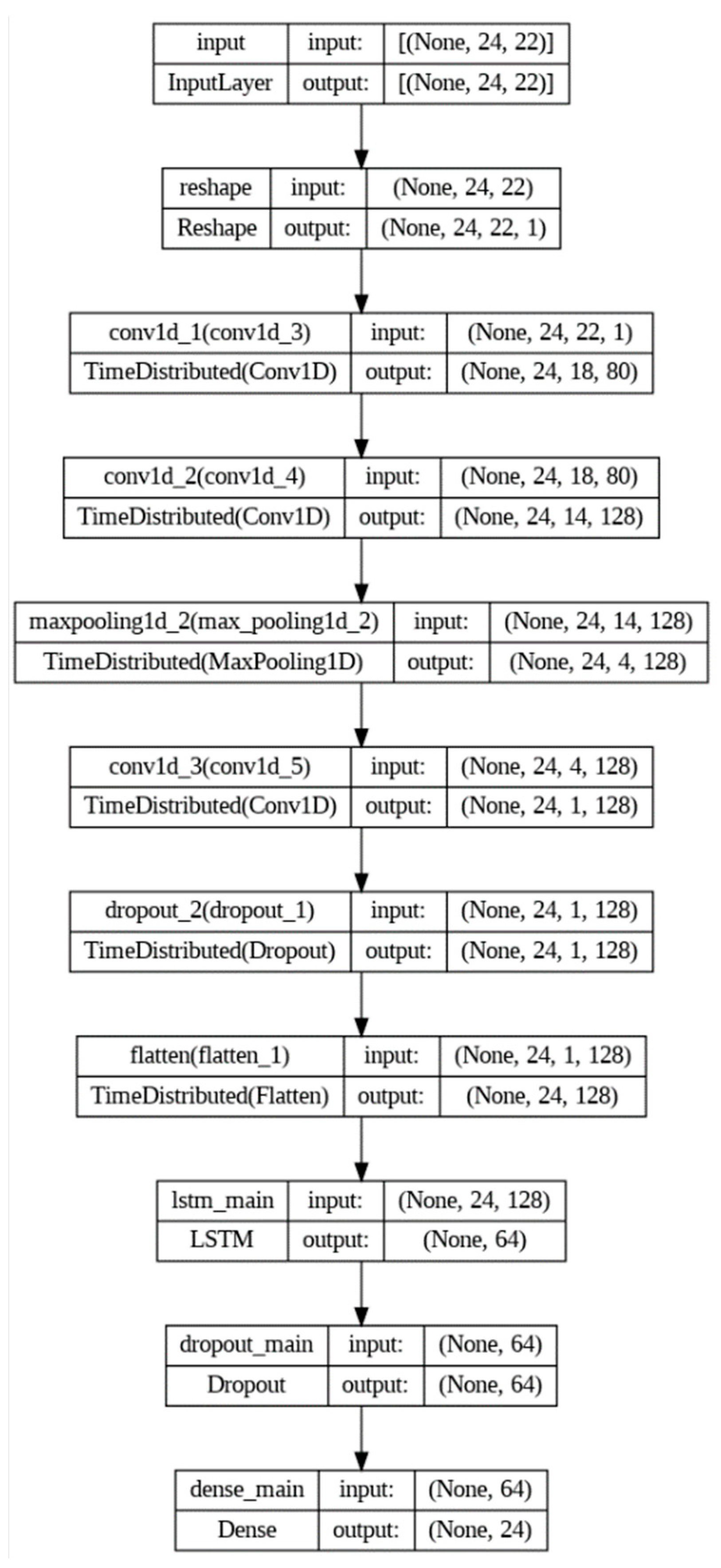
The resulting optimised CNN-LSTM model architecture is shown in Figure 3. The CNN section consisted of three 1D-convolutional layers of 80, 128 and 128 filters, and kernel sizes of 5, 5, and 4, respectively. All convolutional layers were implemented with exponential linear unit (ELU) activation functions. A one-dimensional max-pooling layer with a pool size of 3 was used after the first two convolutional layers and a dropout layer with a drop rate of 0.5 before the flatten layer. The LSTM section consisted of one LSTM layer of 64 units, followed by a dropout layer with a 0.6 rate, and a dense layer of 24 units representing the 24 h of the forecast period.
3.3. Decompensation Risk Curve Prediction and Decompensation Score
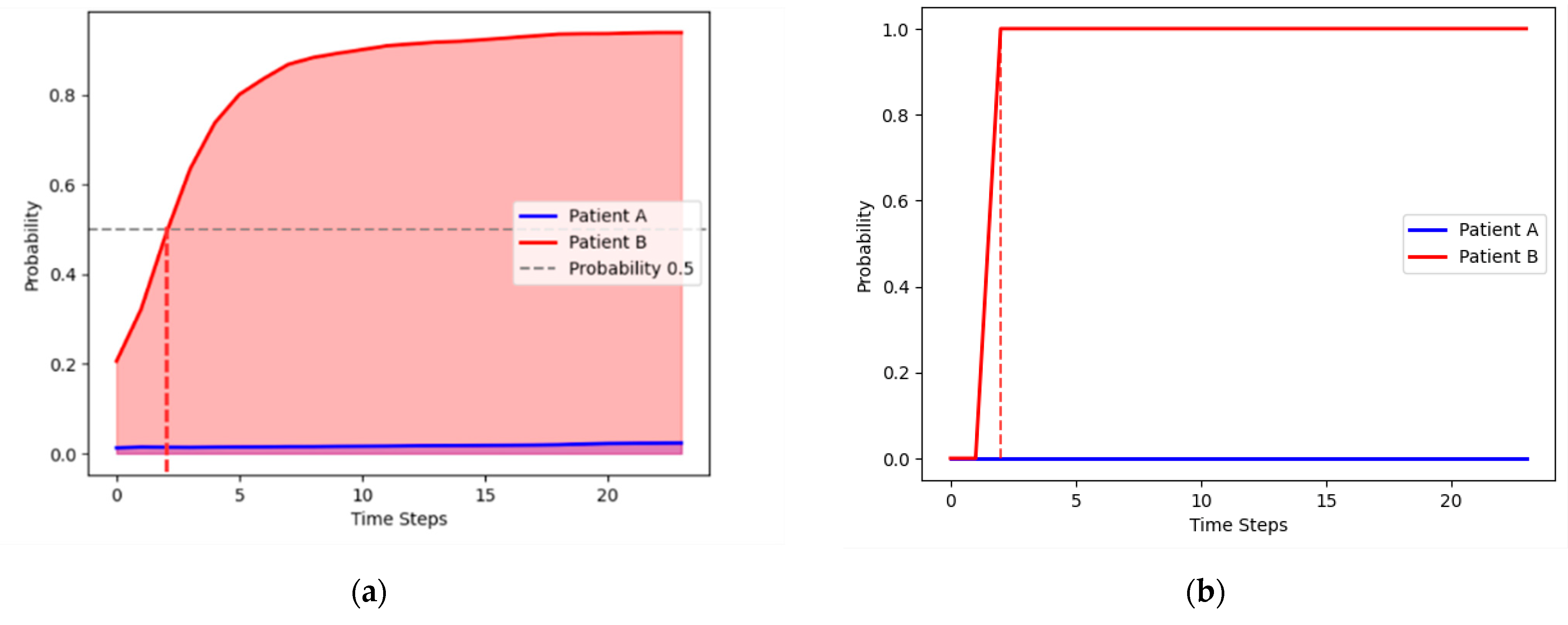
Figure 4 illustrates the resulting decompensation risk curves for two patients, which were predicted by the CNN-LSTM model: patient A, who survived the forecast period and patient B who decompensated at the 3rd hour. Their corresponding decompensation scores, calculated as the area under the decompensation curves are 0.40 and 19.1 for patients A and B, respectively.
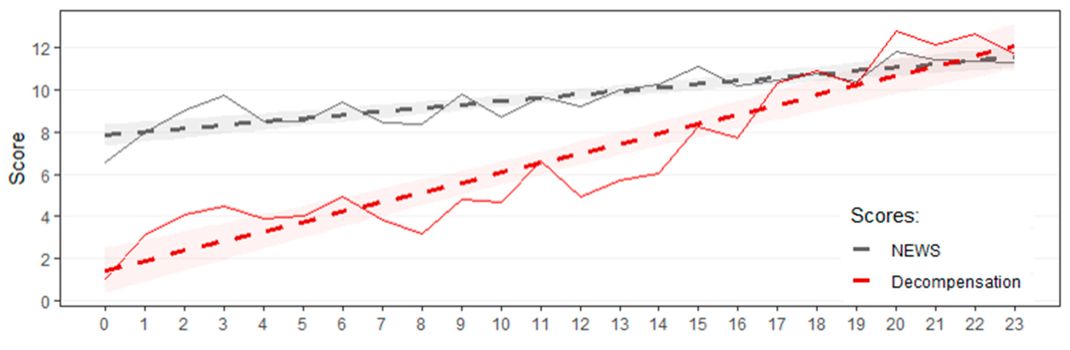
The results of the comparison between our proposed decompensation score and the standard NEWS score are displayed in Figure 5. Both scores are compared against the true decompensation score, derived from the area under the actual decompensation curve. The figure suggests that, while both scores respond similarly in patients at high risk of decompensation, our proposed score appears to be closer to the actual score values than NEWS in low-risk patients.
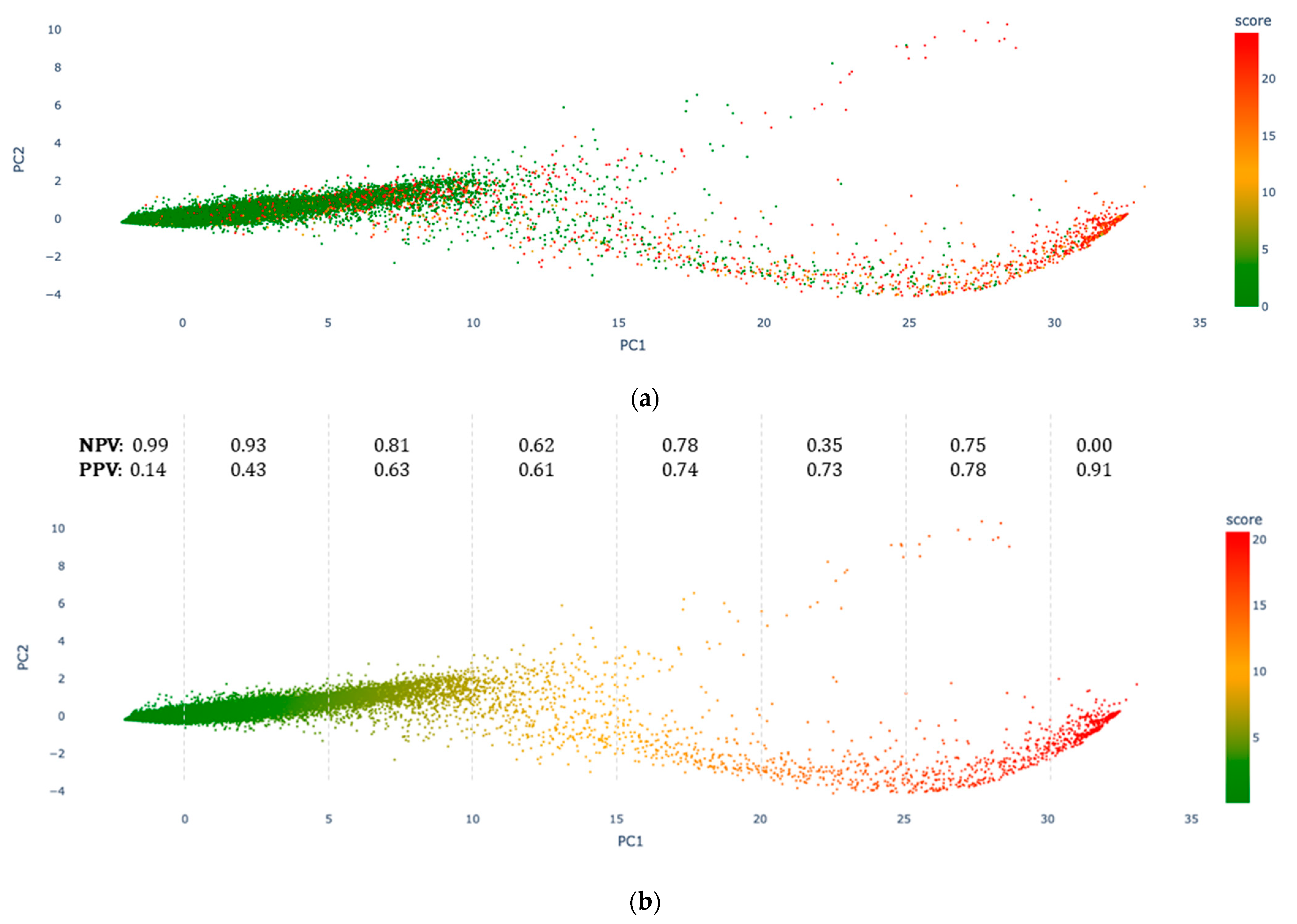
Figure 6 shows the resulting 1st vs. 2nd principal component scatter plot after performing PCA on the dataset formed with the predicted decompensation risk curves for all patient admissions. Between the first two PCs, the PCA model explained 98.3% of the new data variance. Figure 6a shows the true decompensation score, whilst Figure 6b shows the predicted one. As seen in the figure, true and predicted decompensation scores are highly correlated, aligning with the reported performance of the CNN-LSTM model. We calculated the PPV and NPV of the decompensation score. Similar to NEWS, decompensation score values were divided into two classes: high risk of decompensation, with scores greater than 10 (the positive class), and low risk of decompensation, with scores less than 10 (the negative class). Overall, we obtained a PPV of 0.83 and an NPV of 0.96. Additionally, the 1st PC was divided into equal-length segments, and PPVs and NPVs were calculated for each segment. Figure 6b also displays the corresponding PPVs and NPVs. In the same figure, note that the low PPV (0.14) for 1st PC values less than 0 and the low NPV (0.00) for 1st PC values greater than 30 are due to the very small size of the positive and negative classes in those segments, respectively.
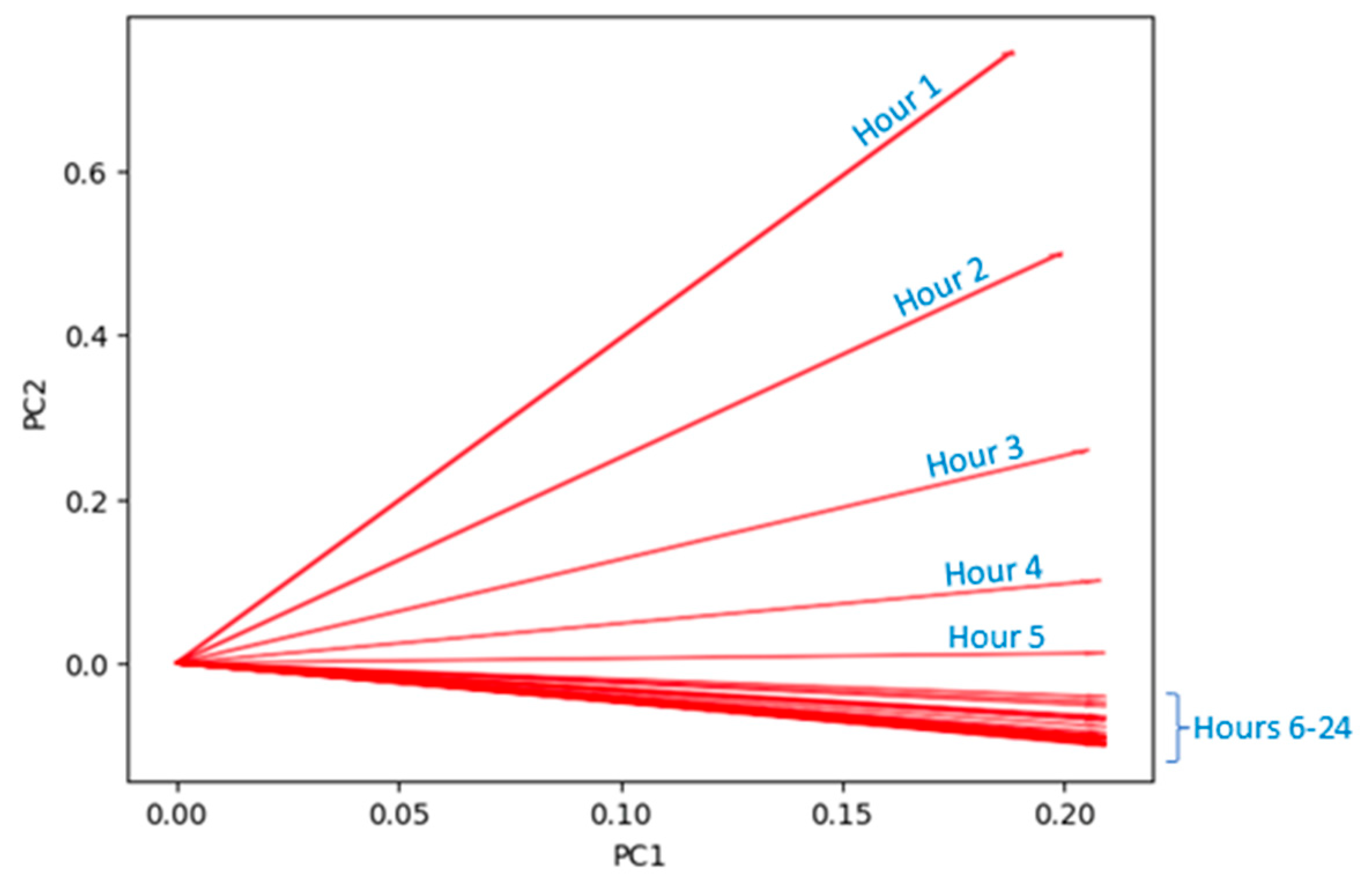
Figure 7 shows the resulting PCA loadings plot, with the PCA loadings corresponding to the predicted hours for decompensation onset. The figure indicates that the first PC is mainly influenced by decompensation risk predictions between hours 4 and later, whilst risks predicted in the first three hours influence both PCs. This suggests that decompensations starting within the first 4 h could follow a different pattern than when decompensation occurs in the final hours of the forecast period.
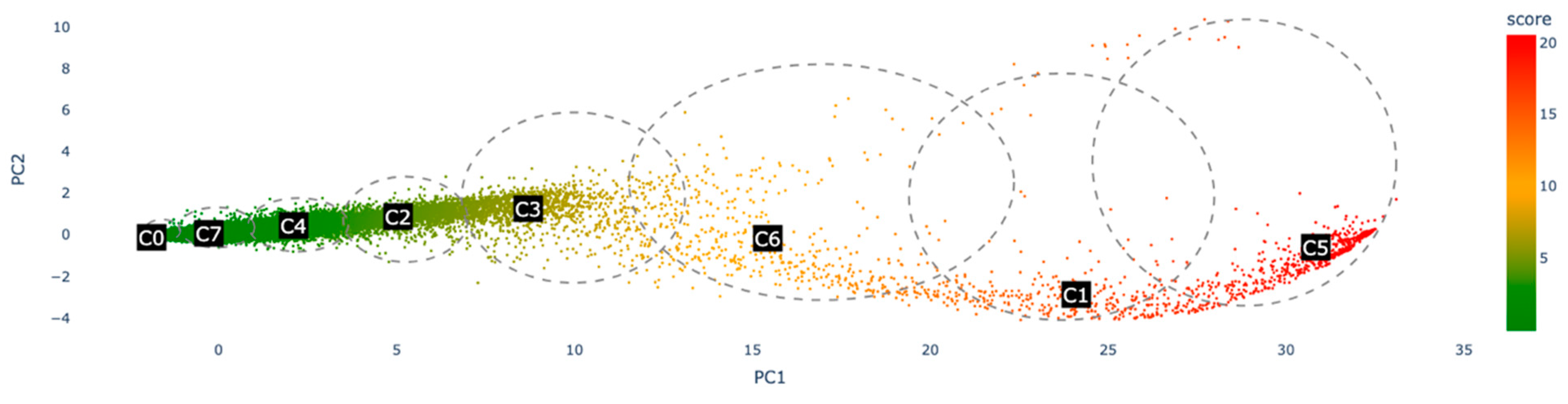
We performed k-means on the PCA-projected data. After using the elbow method, k-means segmented the predicted decompensation risks into seven clusters. The results are shown in Figure 8. It can be seen that admissions with the highest decompensation scores are primarily grouped in clusters C5 and C1, whilst clusters C0 and C7 represent admissions with the lowest scores.
3.4. Model Interpretability
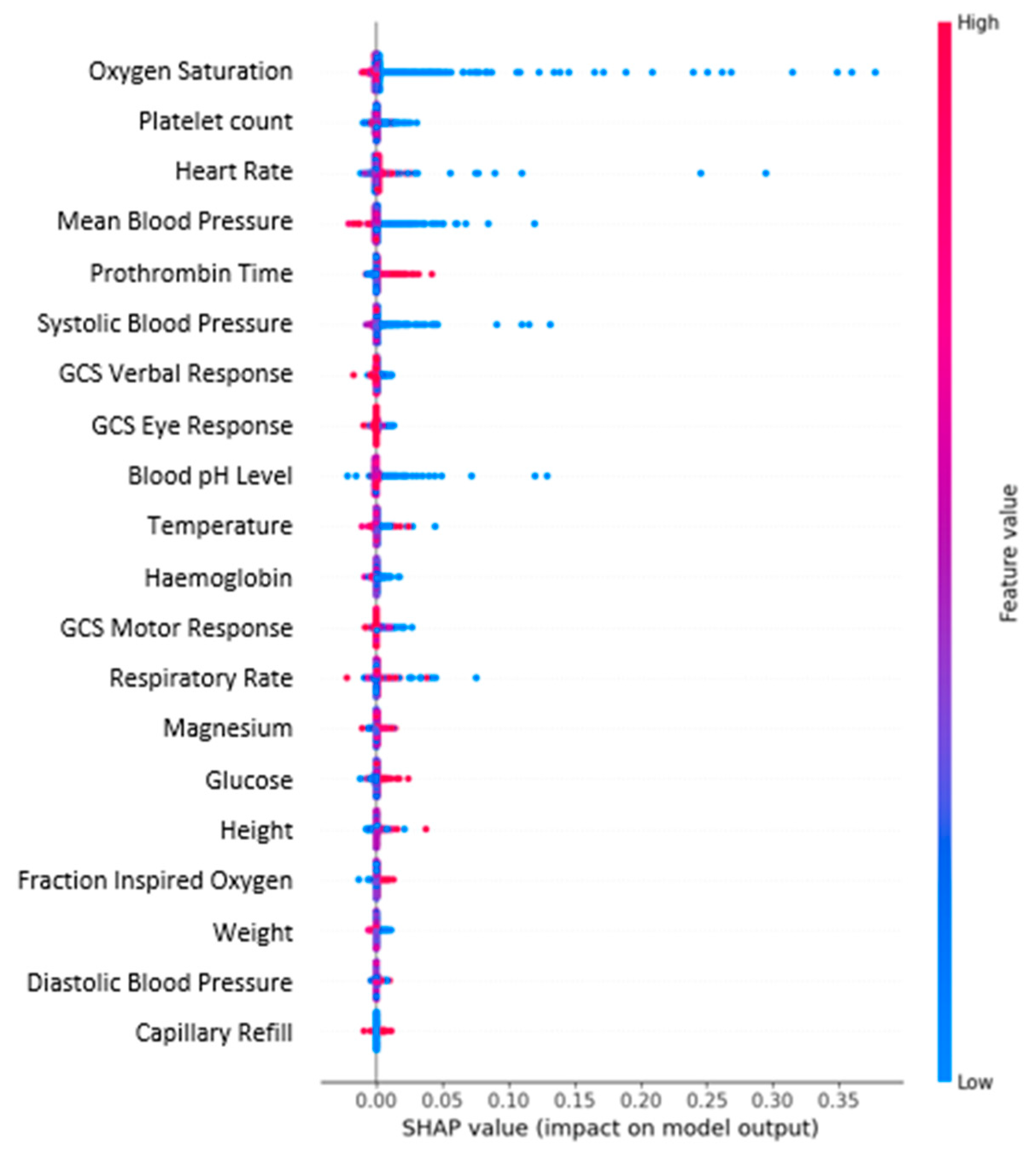
The resulting overall SHAP plot corresponding to the CNN-LSTM model is displayed in Figure 9. From the figure, it was estimated that Oxygen Saturation was the most relevant variable in predicting the decompensation risk, followed by Platelet Count, Heart Rate, Mean Blood Pressure, and Prothrombin Time. Variables such as Capillary Refill, Diastolic Blood Pressure and Weight were found to be the least relevant. It is also noticeable that lower Oxygen Saturation values increase the decompensation risk.
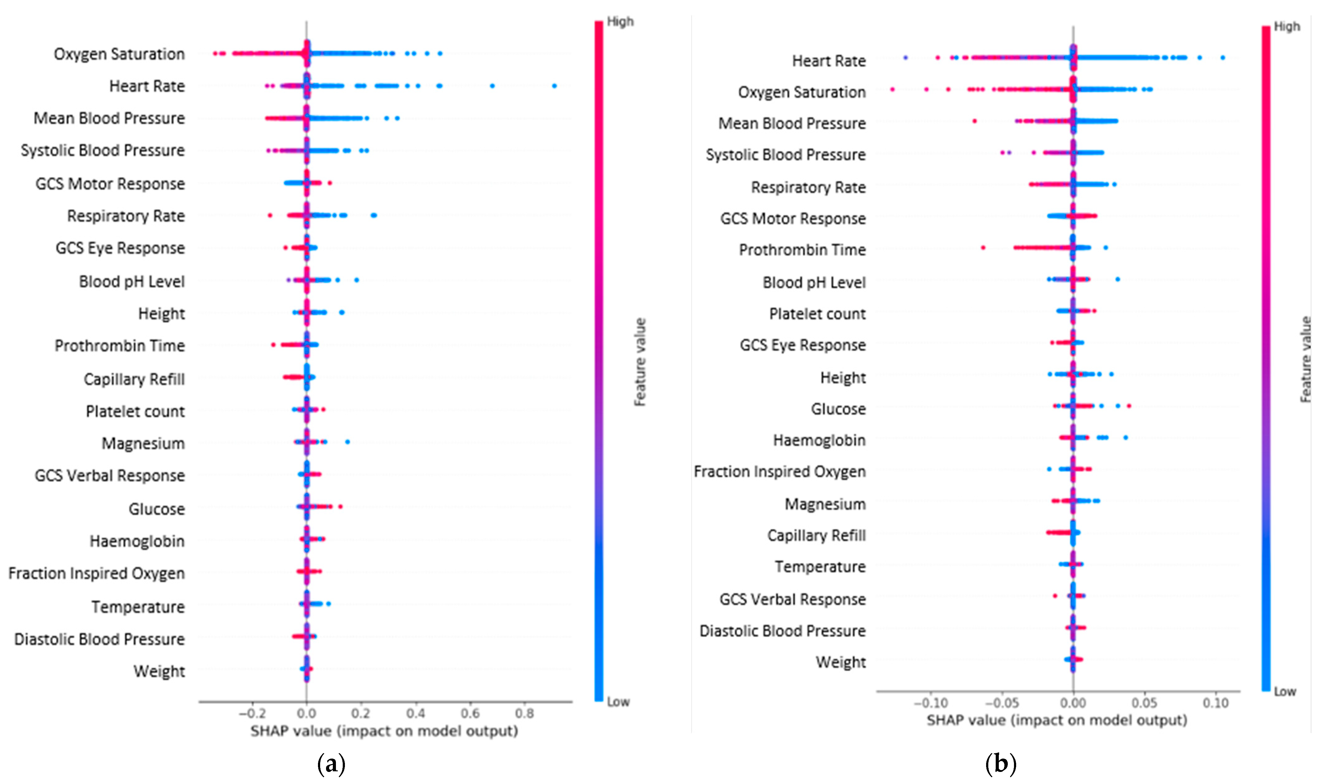
SHAP values were also calculated for clusters C0 and C5, which seemed to be the most dissimilar. Figure 10 displays their resulting SHAP plots. The figure suggests that although a low oxygen saturation value is a critical factor overall, a decrease in a patient’s heart rate could be the most relevant factor in indicating a sudden patient decompensation (first hours).
4. Discussion
4.1. Model Selection and Explanation
This study found that the CNN-LSTM model outperformed the LSTM model in predicting a sequence of decompensation risks, although the performance differences were not significant. We also observed that traditional ML models, particularly RF, demonstrated comparable performance, although their task was to predict the risk of an event within the forecast window rather than a sequence. These results are equivalent to those reported in [2,3,11], although the tasks are slightly different, i.e., a different set of variables were used, or their datasets were extracted from sources other than MIMIC-IV.
To the best of our knowledge, no prior published work has attempted to predict a sequence of decompensation risks rather than single events. This is a critical point, as decompensation is particularly challenging to identify, especially at its early stages. Predicting a sequence facilitates early detection of increased decompensation risk and pace, potentially leading to saving more lives.
This manuscript also introduces a novel decompensation score, calculated as the area under the curve of the decompensation risk sequence. A decompensation score could provide clinicians with a single value, ranging from 0 (indicating the lowest risk) to 24 (highest risk), enabling decompensation monitoring of patients during their stays in the ICU. This proposed score is innovative in that it summarises the risk of decompensation over a time period (e.g., 24 h) rather than a single event. Our score not only provides insight into the severity of the risk but also its proximity.
To understand the logic behind the CNN-LSTM model’s predictions, we performed PCA and k-means on the model predictions. In this way, predicted decompensation risks were stratified into several clusters in terms of their severity. We performed a SHAP analysis on the overall model to find associations between the input features and the decompensation risk.
Furthermore, a similar analysis was carried out on two selected clusters, representing two levels of decompensation severity, to investigate changes in feature importance and the associations with the predicted decompensation risk. We found differences in the features associated with decompensation risk, depending on the specific risk cluster. These results are significant as they suggest that clinical and physiological mechanisms leading to decompensation may be time-varying. Nevertheless, we acknowledge that further investigation is needed. The results, however, indicate that the proposed methodological approach is useful not only in predicting risk but also in providing valuable insights into the reasons behind the model’s predictions.
4.2. Key Risk Factors in Decompensation Prediction
The CNN-LSTM model highlights that variables such as oxygen saturation, prothrombin time (PT), platelet count, heart rate, and blood pressure are key risk factors of decompensation, as shown in Figure 8.
Reduced oxygen saturation has also been previously identified as one of the factors associated with clinical deterioration [19,20,21]. In the case of PT, high levels of it can be associated with patient deterioration [22,23,24], but the significance and appropriate response depend on the individual patient’s medical history and the underlying causes of the elevated PT.
Platelet count is not typically considered a decompensation marker on its own, although abnormalities in platelet count can indicate various medical conditions, e.g., a low platelet count is common in patients with cirrhosis, and it may indicate a more serious and advanced nature of the condition and an increased risk of complications [25,26]. Abnormal platelet counts can also be related to cancer, and cancer patients who are critically ill may be more susceptible to decompensation compared to individuals without cancer [27,28]. Elevated platelet counts (thrombocytosis, greater than 450 × 109/L) can be a marker for potential cancer, including lung, endometrial, gastric, oesophageal, or colorectal cancer. The association of low platelet count (thrombocytopenia, below 150 × 109/L) with cancer includes systemic chemotherapy, radiation, metastatic cancer, and haematological malignancies [29,30].
Both low and high heart rates can be associated with patient decompensation, but the significance of heart rate abnormalities depends on the clinical context and underlying causes. Low heart rate (bradycardia) can be a sign of decompensation in certain situations [31], especially if it leads to reduced cardiac output and insufficient blood supply to vital organs. It can be associated with conditions like heart block, severe conduction system abnormalities, or drug toxicity, which may contribute to decompensation. High heart rate (tachycardia) can also be associated with decompensation, particularly if it results from underlying heart disease or other medical conditions [32,33,34,35], e.g., atrial fibrillation [36,37,38,39], ventricular tachycardia [40,41], or severe systemic infection [23,42], which may contribute to decompensation.
Blood pressure can be an important factor in assessing the risk of patient decompensation, particularly in the context of cardiovascular health [43,44]. Prolonged hypertension can contribute to chronic vascular damage and increase the risk of conditions like stroke [45], heart attack [43,44], kidney disease [46,47], and vascular diseases [48,49]. While hypertension itself is not a direct marker of decompensation, it is a risk factor for the development of various cardiovascular and cerebrovascular complications, which can lead to decompensation. Hypotension, in turn, can be associated with conditions such as shock [50], heart failure [51], or sepsis [52], and it is considered a risk factor for decompensation in these cases. In ICU patients, hypotension can be indicative of various underlying issues and can lead to complications [52,53], including multi-organ failure, cerebral hypoperfusion, and poor outcomes.
4.3. Limitations of the Study
Our study has several limitations, primarily related to the dataset and the data recorded in the database. Notably, MIMIC-IV lacks a precise definition for ICU patient decompensation. Similar to other studies, we used the risk of death as a proxy. However, it is possible that certain events leading to patient death may not be directly correlated with health decompensation. While a patient can recover from decompensation, they cannot recover from death.
Another limitation arises from the exclusion of patients with ICU stays of less than 24 h, which may introduce potential sampling bias. Selecting the right length for the time series is a trade-off between patient inclusion and the number of time points per time series, both of which can potentially affect model performance. It is also important to note that SHAP analysis can only suggest potential associations between input characteristics and predictions, which is not the same as stating causation. This means that further research is needed to identify potential confounding factors if such causal links are to be established.
Furthermore, clinical data often exhibit high levels of missing values and noise, which commonly limit the performance of any data-driven model, regardless of the ML techniques used. The choice of vitals and other factors is also very important in the development of any score, in our case, a decompensation score. Since the aim of our paper was to propose a methodology that would enable the development of such a score, we used publicly available data from the MIMIC-IV database. However, we recognise that further work will be required, including not only a revision of the choice of variables but also further testing in prospective patient cohorts. Importantly, special consideration must be given to the selection of the missing value imputation method, as it can impact both model performance and the quality of the proposed score. In this study, we opted for the same imputation method as the one used in [11] since both studies use similar data sources and settings. However, imputation methods that could be more appropriate for time series should also be explored in further analyses.
5. Conclusions
Our study confirms the effectiveness of ML models in predicting ICU decompensation. A key contribution of our research lies in the prediction of a sequence of decompensation risks rather than a single event. Additionally, our study introduces a novel decompensation score, derived from the predicted sequences, which could potentially offer clinicians a more robust tool for monitoring and early detection of patient decompensation, thereby potentially saving more lives.
Author Contributions
I.O. conceptualised the methodological approach and led the study. N.A. implemented the code and ran the experiments. S.O.-M. contributed to the discussions. N.A. drafted the early version of the manuscript. I.O and S.O.-M. wrote, reviewed and edited the final manuscript. All authors have read and agreed to the published version of the manuscript.
Funding
This research received no external funding.
Data Availability Statement
MIMIC-IV is an open-access database, which is available from https://physionet.org/content/mimiciv/2.2/ (accessed on 2 October 2023).
Conflicts of Interest
The authors declare no conflict of interest.
References
- Veldhuis, L.I.; Woittiez, N.J.C.; Nanayakkara, P.W.B.; Ludikhuize, J. Artificial Intelligence for the Prediction of In-Hospital Clinical Deterioration: A Systematic Review. Crit. Care Explor. 2022, 4, e0744. [Google Scholar] [CrossRef] [PubMed]
- Kia, A.; Timsina, P.; Joshi, H.N.; Klang, E.; Gupta, R.R.; Freeman, R.M.; Reich, D.L.; Tomlinson, M.S.; Dudley, J.T.; Kohli-Seth, R.; et al. MEWS++: Enhancing the prediction of clinical deterioration in admitted patients through a machine learning model. J. Clin. Med. 2020, 9, 343. [Google Scholar] [CrossRef] [PubMed]
- Ruiz, V.M.; Goldsmith, M.P.; Shi, L.; Simpao, A.F.; Gálvez, J.A.; Naim, M.Y.; Nadkarni, V.; Gaynor, J.W.; Tsui, F. Early prediction of clinical deterioration using data-driven machine-learning modeling of electronic health records. J. Thorac. Cardiovasc. Surg. 2022, 164, 211–222.e3. [Google Scholar] [CrossRef] [PubMed]
- Thorsen-Meyer, H.-C.; Nielsen, A.B.; Nielsen, A.P.; Kaas-Hansen, B.S.; Toft, P.; Schierbeck, J.; Strøm, T.; Chmura, P.J.; Heimann, M.; Dybdahl, L.; et al. Dynamic and explainable machine learning prediction of mortality in patients in the intensive care unit: A retrospective study of high-frequency data in electronic patient records. Lancet Digit. Health 2020, 2, e179–e191. [Google Scholar] [CrossRef]
- Ho, L.V.; Aczon, M.; Ledbetter, D.; Wetzel, R. Interpreting a recurrent neural network’s predictions of ICU mortality risk. J. Biomed. Inform. 2021, 114, 103672. [Google Scholar] [CrossRef]
- Leung, K.K.; Rooke, C.; Smith, J.; Zuberi, S.; Volkovs, M. Temporal Dependencies in Feature Importance for Time Series Predictions. arxiv 2021, arXiv:2107.14317. [Google Scholar]
- Van Houdt, G.; Mosquera, C.; Nápoles, G. A review on the long short-term memory model. Artif. Intell. Rev. 2020, 53, 5929–5955. [Google Scholar] [CrossRef]
- Solares, J.R.A.; Raimondi, F.E.D.; Zhu, Y.; Rahimian, F.; Canoy, D.; Tran, J.; Gomes, A.C.P.; Payberah, A.H.; Zottoli, M.; Nazarzadeh, M.; et al. Deep learning for electronic health records: A comparative review of multiple deep neural architectures. J. Biomed. Inform. 2020, 101, 103337. [Google Scholar] [CrossRef]
- Johnson, A.E.W.; Bulgarelli, L.; Shen, L.; Gayles, A.; Shammout, A.; Horng, S.; Pollard, T.J.; Hao, S.; Moody, B.; Gow, B.; et al. MIMIC-IV, a freely accessible electronic health record dataset. Sci. Data 2023, 10, 1. [Google Scholar] [CrossRef]
- Shao, J.; Zhong, B. Last observation carry-forward and last observation analysis. Stat. Med. 2003, 22, 2429–2441. [Google Scholar] [CrossRef]
- Harutyunyan, H.; Khachatrian, H.; Kale, D.C.; Ver Steeg, G.; Galstyan, A. Multitask learning and benchmarking with clinical time series data. Sci. Data 2019, 6, 96. [Google Scholar] [CrossRef] [PubMed]
- Bishop, C.M. Pattern Recognition and Machine Learning, 3rd ed.; Springer: New York, NY, USA, 2006. [Google Scholar]
- Murugan, P. Learning the Sequential Temporal Information with Recurrent Neural Networks. arXiv 2018, arXiv:1807.02857. [Google Scholar]
- Livieris, I.E.; Pintelas, E.; Pintelas, P. A CNN–LSTM model for gold price time-series forecasting. Neural Comput. Appl. 2020, 32, 17351–17360. [Google Scholar] [CrossRef]
- Youden, W.J. Index for rating diagnostic tests. Cancer 1950, 3, 32–35. [Google Scholar] [CrossRef]
- Williams, B. The National Early Warning Score: From concept to NHS implementation. Clin. Med. J. R. Coll. Physicians Lond. 2022, 22, 499. [Google Scholar] [CrossRef]
- Molnar. 9.6 SHAP (SHapley Additive Explanations). A Guide for Making Black Box Models Explainable. 2021. Available online: https://christophm.github.io/interpretable-ml-book (accessed on 2 November 2023).
- Jeyakumar, J.V.; Noor, J.; Cheng, Y.H.; Garcia, L.; Srivastava, M. How can I explain this to you? An empirical study of deep neural network explanation methods. Adv. Neural Inf. Process. Syst. 2020, 33, 4211–4222. [Google Scholar]
- Kabrhel, C.; Okechukwu, I.; Hariharan, P.; Takayesu, J.K.; MacMahon, P.; Haddad, F.; Chang, Y. Factors associated with clinical deterioration shortly after PE. Thorax 2014, 69, 835–842. [Google Scholar] [CrossRef]
- Yan, B.; Song, L.; Guo, J.; Wang, Y.; Peng, L.; Li, D. Association Between Clinical Characteristics and Short-Term Outcomes in Adult Male COVID-19 Patients With Mild Clinical Symptoms: A Single-Center Observational Study. Front. Med. 2021, 7, 571396. [Google Scholar] [CrossRef]
- Lee, J.-R.; Jung, Y.-K.; Hong, S.-B.; Huh, J.W. Predictors of Repeat Medical Emergency Team Activation in Deteriorating Ward Patients: A Retrospective Cohort Study. J. Clin. Med. 2022, 11, 1736. [Google Scholar] [CrossRef]
- Billoir, P.; Alexandre, K.; Duflot, T.; Roger, M.; Miranda, S.; Goria, O.; Joly, L.M.; Demeyere, M.; Feugray, G.; Brunel, V.; et al. Investigation of Coagulation Biomarkers to Assess Clinical Deterioration in SARS-CoV-2 Infection. Front. Med. 2021, 8, 670694. [Google Scholar] [CrossRef]
- Ortega-Martorell, S.; Olier, I.; Johnston, B.W.; Welters, I.D. Sepsis-induced coagulopathy is associated with new episodes of atrial fibrillation in patients admitted to critical care in sinus rhythm. Front. Med. 2023, 10, 1230854. [Google Scholar] [CrossRef]
- Tekle, E.; Gelaw, Y.; Dagnew, M.; Gelaw, A.; Negash, M.; Kassa, E.; Bizuneh, S.; Wudineh, D.; Asrie, F. Risk stratification and prognostic value of prothrombin time and activated partial thromboplastin time among COVID-19 patients. PLoS ONE 2022, 17, e0272216. [Google Scholar] [CrossRef]
- Sigal, S.H.; Sherman, Z.; Jesudian, A. Clinical Implications of Thrombocytopenia for the Cirrhotic Patient. Hepatic Med. Evid. Res. 2020, 12, 49–60. [Google Scholar] [CrossRef]
- Surana, P.; Hercun, J.; Takyar, V.; Kleiner, D.E.; Heller, T.; Koh, C. Platelet count as a screening tool for compensated cirrhosis in chronic viral hepatitis. World J. Gastrointest. Pathophysiol. 2021, 12, 40–50. [Google Scholar] [CrossRef]
- Martos-Benítez, F.D.; Soler-Morejón, C.d.D.; Lara-Ponce, K.X.; Orama-Requejo, V.; Burgos-Aragüez, D.; Larrondo-Muguercia, H.; Lespoir, R.W. Critically ill patients with cancer: A clinical perspective. World J. Clin. Oncol. 2020, 11, 809–835. [Google Scholar] [CrossRef]
- Schellongowski, P.; Sperr, W.R.; Wohlfarth, P.; Knoebl, P.; Rabitsch, W.; Watzke, H.H.; Staudinger, T. Critically ill patients with cancer: Chances and limitations of intensive care medicine—A narrative review. ESMO Open 2016, 1, e000018. [Google Scholar] [CrossRef]
- NICE. Platelets—Abnormal Counts and Cancer|Clinical Knowledge Summary|National Institute for Health and Care Excellence (NICE). 2021. Available online: https://cks.nice.org.uk/topics/platelets-abnormal-counts-cancer/ (accessed on 1 November 2023).
- Mounce, L.T.; Hamilton, W.; Bailey, S.E. Cancer incidence following a high-normal platelet count: Cohort study using electronic healthcare records from English primary care. Br. J. Gen. Pract. 2020, 70, e622–e628. [Google Scholar] [CrossRef]
- Aoun, M.; Tabbah, R. Case report: Severe bradycardia, a reversible cause of “Cardio-Renal-Cerebral Syndrome”. BMC Nephrol. 2016, 17, 162. [Google Scholar] [CrossRef]
- Mozos, I. Arrhythmia risk in liver cirrhosis. World J. Hepatol. 2015, 7, 662–672. [Google Scholar] [CrossRef]
- Lu, X.; Wang, Z.; Yang, L.; Yang, C.; Song, M. Risk Factors of Atrial Arrhythmia in Patients With Liver Cirrhosis: A Retrospective Study. Front. Cardiovasc. Med. 2021, 8, 704073. [Google Scholar] [CrossRef]
- Teerlink, J.R.; Alburikan, K.; Metra, M.; Rodgers, J.E. Acute Decompensated Heart Failure Update. Curr. Cardiol. Rev. 2015, 11, 53–62. [Google Scholar] [CrossRef] [PubMed]
- Rosano, G.M.; Moura, B.; Metra, M.; Böhm, M.; Bauersachs, J.; Ben Gal, T.; Adamopoulos, S.; Abdelhamid, M.; Bistola, V.; Čelutkienė, J.; et al. Patient profiling in heart failure for tailoring medical therapy. A consensus document of the Heart Failure Association of the European Society of Cardiology. Eur. J. Heart Fail. 2021, 23, 872–881. [Google Scholar] [CrossRef]
- DiMarco, J.P. Atrial Fibrillation and Acute Decompensated Heart Failure. Circ. Heart Fail. 2009, 2, 72–73. [Google Scholar] [CrossRef]
- Ortega-Martorell, S.; Pieroni, M.; Johnston, B.W.; Olier, I.; Welters, I.D. Development of a Risk Prediction Model for New Episodes of Atrial Fibrillation in Medical-Surgical Critically Ill Patients Using the AmsterdamUMCdb. Front. Cardiovasc. Med. 2022, 9, 897709. [Google Scholar] [CrossRef]
- Mendes, F.d.S.N.S.; Atié, J.; Garcia, M.I.; Gripp, E.d.A.; de Sousa, A.S.; Feijó, L.A.; Xavier, S.S. Atrial fibrillation in decompensated heart failure: Associated factors and in-hospital outcome. Arq. Bras. Cardiol. 2014, 103, 315–322. [Google Scholar] [CrossRef]
- Park, J.J.; Lee, H.; Kim, K.H.; Yoo, B.; Kang, S.; Baek, S.H.; Jeon, E.; Kim, J.; Cho, M.; Chae, S.C.; et al. Heart failure and atrial fibrillation: Tachycardia-mediated acute decompensation. ESC Heart Fail. 2021, 8, 2816–2825. [Google Scholar] [CrossRef]
- Muser, D.; Castro, S.A.; Liang, J.J.; Santangeli, P. Identifying risk and management of acute haemodynamic decompensation during catheter ablation of ventricular tachycardia. Arrhythmia Electrophysiol. Rev. 2018, 7, 282–287. [Google Scholar] [CrossRef]
- Wichterle, D.; Peichl, P.; Stojadinovic, P.; Haskova, J.; Borisincova, E.; Sevcik, A.; Sincakova, E.; Kotyza, V.; Cihak, R.; Kautzner, J. Periprocedural acute hemodynamic decompensation associated with substrate-based ablation of ventricular tachycardia in patients with structural heart disease—Rare and nonpredictable event. Europace 2023, 25, euad122-339. [Google Scholar] [CrossRef]
- Bezati, S.; Velliou, M.; Ventoulis, I.; Simitsis, P.; Parissis, J.; Polyzogopoulou, E. Infection as an under-recognized precipitant of acute heart failure: Prognostic and therapeutic implications. Heart Fail. Rev. 2023, 28, 893–904. [Google Scholar] [CrossRef]
- Oh, G.C.; Cho, H.-J. Blood pressure and heart failure. Clin. Hypertens. 2020, 26, 1. [Google Scholar] [CrossRef]
- Wu, C.-Y.; Hu, H.-Y.; Chou, Y.-J.; Huang, N.; Chou, Y.-C.; Li, C.-P. High Blood Pressure and All-Cause and Cardiovascular Disease Mortalities in Community-Dwelling Older Adults. Medicine 2015, 94, e2160. [Google Scholar] [CrossRef]
- Wajngarten, M.; Silva, G.S. Hypertension and Stroke: Update on Treatment. Eur. Cardiol. Rev. 2019, 14, 111–115. [Google Scholar] [CrossRef]
- Lee, H.; Kwon, S.H.; Jeon, J.S.; Noh, H.; Han, D.C.; Kim, H. Association between blood pressure and the risk of chronic kidney disease in treatment-naïve hypertensive patients. Kidney Res. Clin. Pract. 2022, 41, 31–42. [Google Scholar] [CrossRef]
- Vaes, B.; Beke, E.; Truyers, C.; Elli, S.; Buntinx, F.; Verbakel, J.Y.; Goderis, G.; Van Pottelbergh, G. The correlation between blood pressure and kidney function decline in older people: A registry-based cohort study. BMJ Open 2015, 5, e007571. [Google Scholar] [CrossRef]
- Nazarzadeh, M.; Bidel, Z.; Mohseni, H.; Canoy, D.; Pinho-Gomes, A.-C.; Hassaine, A.; Dehghan, A.; Tregouet, D.-A.; Smith, N.L.; Rahimi, K.; et al. Blood pressure and risk of venous thromboembolism: A cohort analysis of 5.5 million UK adults and Mendelian randomization studies. Cardiovasc. Res. 2022, 119, 835–842. [Google Scholar] [CrossRef]
- Hibino, M.; Otaki, Y.; Kobeissi, E.; Pan, H.; Hibino, H.; Taddese, H.; Majeed, A.; Verma, S.; Konta, T.; Yamagata, K.; et al. Blood Pressure, Hypertension, and the Risk of Aortic Dissection Incidence and Mortality: Results From the J-SCH Study, the UK Biobank Study, and a Meta-Analysis of Cohort Studies. Circulation 2022, 145, 633–644. [Google Scholar] [CrossRef]
- Vahdatpour, C.; Collins, D.; Goldberg, S. Cardiogenic Shock. J. Am. Heart Assoc. 2019, 8, e011991. [Google Scholar] [CrossRef]
- Jones, C.D.; Loehr, L.R.; Franceschini, N.; Rosamond, W.D.; Chang, P.P.; Shahar, E.; Couper, D.J.; Rose, K.M. Orthostatic hypotension as a risk factor for incident heart failure: The atherosclerosis risk in communities study. Hypertension 2012, 59, 913–918. [Google Scholar] [CrossRef]
- Maheshwari, K.; Nathanson, B.H.; Munson, S.H.; Khangulov, V.; Stevens, M.; Badani, H.; Khanna, A.K.; Sessler, D.I. The relationship between ICU hypotension and in-hospital mortality and morbidity in septic patients. Intensiv. Care Med. 2018, 44, 857–867. [Google Scholar] [CrossRef]
- van der Ven, W.; Schuurmans, J.; Schenk, J.; Roerhorst, S.; Cherpanath, T.; Lagrand, W.; Thoral, P.; Elbers, P.; Tuinman, P.; Scheeren, T.; et al. Monitoring, management, and outcome of hypotension in Intensive Care Unit patients, an international survey of the European Society of Intensive Care Medicine. J. Crit. Care 2021, 67, 118–125. [Google Scholar] [CrossRef]
Figure 1.
Methodological approach implemented for this study. (a) Displays the input (e.g., vitals, lab tests, etc.) sequences that the DL models take and the output (decompensation risk) sequence that they forecast. A decompensation score is calculated as the area under the decompensation risk sequence (b).

Figure 2.
Optimised LSTM model architecture.

Figure 3.
Optimised CNN-LSTM model architecture.

Figure 4.
Comparison of decompensation risk curves between two patients. (a) Predicted curves. (b) Actual curves.
Figure 4.
Comparison of decompensation risk curves between two patients. (a) Predicted curves. (b) Actual curves.

Figure 5.
Comparison between NEWS and our proposed decompensation scores. Horizontal axis corresponds to the true decompensation score, while the vertical axis corresponds to the estimated scores. Average score values are represented by continuous lines, whilst calculated linear trends, by dashed lines. Shades around trend lines represent 95% confidence intervals.

Figure 6.
PCA visualisation of CNN-LSTM model’s 24-h predictions. (a) True decompensation scores overlaid. (b) Predicted scores. Calculated PPV and NPV for each PC1 segment are shown on top of (b).
Figure 6.
PCA visualisation of CNN-LSTM model’s 24-h predictions. (a) True decompensation scores overlaid. (b) Predicted scores. Calculated PPV and NPV for each PC1 segment are shown on top of (b).

Figure 7.
PCA loadings plot. PCA loadings (hours in the predicted risk data) are represented by the red arrows.
Figure 7.
PCA loadings plot. PCA loadings (hours in the predicted risk data) are represented by the red arrows.

Figure 8.
K-means clusters on the PCA projected risk prediction data.

Figure 9.
Overall SHAP plot of the CNN-LSTM model.

Figure 10.
SHAP plots. (a) Cluster C0. (b) Cluster C5.


Table 1.
Hyperparameter values for the different methods used.
| Method | Hyperparameter | Options |
|---|---|---|
| SVM | Kernel | Radial basis, polynomial and sigmoid |
| Technique | Grid search cross-validation | |
| Gamma | 1, 10, 0.1 and auto | |
| Cost | 1, 0.1 and 0.01 | |
| RF | Bootstrap | True, False |
| Technique | Randomised search cross-validation | |
| Maximum Depth | 10, 20, 30, 40, 50, 60, 70, 80, 90, 100, 110, None | |
| Max features | Auto, sqrt | |
| Minimum leaf samples | 1, 2, 4 | |
| Minimum sample split | 2, 5, 10 | |
| Number of trees | 200, 400, 600, 800, 1000, 1200, 1400, 1600, 1800, 2000 | |
| LSTM | LSTM units | 240, 64, 120 |
| Dropout Layers | 0.5, none | |
| Dense Layers | 180, 100, 24 | |
| CNN-LSTM | Conv1D Filters | 80, 128 |
| Dropout Layers | 0.6, none, 0.7 | |
| MaxPooling1D pool sizes | 3, 5, 1 | |
| Flatten layers | Yes, No | |
| LSTM units | 64 | |
| Dense Layers | 48, 24 | |
| Activation functions | RELU, SELU, ELU |
Table 2.
Description of the variables used in this study. For numeric variables, the median and 1st and 3rd quartile are presented, whilst for binary variables, we present the prevalence (as a percentage). The last two columns display the level of missing values (as a percentage) and the imputed value used, respectively. GCS stands for Glasgow Coma Scale.
| Variable | Statistics | Min, Max | % Missing Values | Imputed Value |
|---|---|---|---|---|
| Age [years] | 67 [55, 77] | 18, 89 | 0 | - |
| Height [cm] | 170 [162.8, 177.9] | 53.2, 231.1 | 55.23 | 170 |
| Weight [kg] | 80.4 [67.6, 96.5] | 32.5, 296.8 | 2.17 | 81 |
| Temperature [°C] | 36.8 [36.6, 37.2] | 23.1, 43.1 | 0.2 | 36.6 |
| Heart Rate [beats per min] | 84.8 [73, 97] | 15, 295 | 0.001 | 86 |
| Respiratory Rate [breaths per min] | 19.5 [16, 23.5] | 5.3, 280 | 0.02 | 19 |
| Fraction Inspired Oxygen [%] | 40 [40, 50] | 20, 100 | 24.44 | 0.21 |
| Oxygen Saturation [%] | 97 [95, 99] | 42, 100 | 0.004 | - |
| GCS Eye Response | 4 [3, 4] | 1, 4 | 0.02 | 4 |
| GCS Motor Response | 6 [5, 6] | 1, 6 | 0.02 | 6 |
| GCS Verbal Response | 4 [1, 5] | 1, 5 | 0.02 | 5 |
| GCS Total Response | 14 [10, 15] | 3, 15 | 0.02 | 15 |
| Glucose [mg/dL] | 128 [107, 159] | 33, 1884 | 0.1 | 128 |
| Haemoglobin [g/dL] | 9.7 [8.5, 11.2] | 4.8, 21.1 | 0.20 | - |
| Platelet count [K/uL] | 190 [128, 270] | 54, 1475 | 0.19 | - |
| Diastolic Blood Pressure [mmHg] | 61 [53, 72] | 34, 338 | 0.01 | 59 |
| Mean Blood Pressure [mmHg] | 77 [68.0, 88] | 14, 330 | 0.01 | 77 |
| Systolic Blood Pressure [mmHg] | 118 [104.5, 134] | 46, 365 | 0.01 | 118 |
| Blood pH Level | 7.41 [7.36, 7.45] | 6.68, 7.93 | 27.54 | 7.4 |
| Capillary Refill [yes] | 4.26% | 0, 1 | 6.95 | 0 |
| Prothrombin Time [sec] | 13.7 [12.4, 16] | 7.1, 100 | 4.90 | 11 |
| Magnesium [mg/dL] | 2.1 [1.9, 2.3] | 1.0, 14.2 | 0.70 | 1.9 |
Table 3.
Model performance results.
| Model | Balanced acc. | PPV | NPV | AUC-PR | AUC-ROC | MCC |
|---|---|---|---|---|---|---|
| LR | 0.65 [0.64, 0.66] | 0.68 [0.66, 0.70] | 0.95 [0.94, 0.96] | 0.43 [0.40, 0.46] | 0.84 [0.80, 0.88] | 0.17 [0.16, 0.18] |
| SVM | 0.61 [0.60, 0.62] | 0.79 [0.78, 0.80] | 0.96 [0.95, 0.97] | 0.44 [0.43, 0.45] | 0.85 [0.83, 0.87] | 0.30 [0.29, 0.31] |
| RF | 0.84 [0.83, 0.85] | 0.80 [0.80, 0.82] | 0.96 [0.96, 0.97] | 0.50 [0.48, 0.53] | 0.88 [0.86, 0.90] | 0.34 [0.33, 0.35] |
| LSTM | 0.82 [0.80, 0.84] | 0.71 [0.70, 0.72] | 0.97 [0.96, 0.98] | 0.49 [0.48, 0.50] | 0.88 [0.86, 0.90] | 0.33 [0.32, 0.34] |
| CNN-LSTM | 0.83 [0.82, 0.84] | 0.80 [0.78, 0.82] | 0.96 [0.95, 0.97] | 0.51 [0.50, 0.52] | 0.90 [0.89, 0.91] | 0.34 [0.33, 0.35] |
Table 4.
Hyperparameter tuning results for SVM and RF.
| Algorithm | Hyperparameter | Best Parameter |
|---|---|---|
| SVM | Kernel | Radial Basis |
| Gamma | 0.01 | |
| Cost | 1 | |
| RF | Bootstrap | True |
| Maximum Depth | 50 | |
| Max features | sqrt | |
| Minimum leaf samples | 2 | |
| Minimum sample split | 10 | |
| Number of trees | 200 |
Disclaimer/Publisher’s Note: The statements, opinions and data contained in all publications are solely those of the individual author(s) and contributor(s) and not of MDPI and/or the editor(s). MDPI and/or the editor(s) disclaim responsibility for any injury to people or property resulting from any ideas, methods, instructions or products referred to in the content. |
© 2023 by the authors. Licensee MDPI, Basel, Switzerland. This article is an open access article distributed under the terms and conditions of the Creative Commons Attribution (CC BY) license (https://creativecommons.org/licenses/by/4.0/).
Share and Cite
MDPI and ACS Style
Aikodon, N.; Ortega-Martorell, S.; Olier, I. Predicting Decompensation Risk in Intensive Care Unit Patients Using Machine Learning. Algorithms 2024, 17, 6. https://doi.org/10.3390/a17010006
AMA Style
Aikodon N, Ortega-Martorell S, Olier I. Predicting Decompensation Risk in Intensive Care Unit Patients Using Machine Learning. Algorithms. 2024; 17(1):6. https://doi.org/10.3390/a17010006
Chicago/Turabian StyleAikodon, Nosa, Sandra Ortega-Martorell, and Ivan Olier. 2024. "Predicting Decompensation Risk in Intensive Care Unit Patients Using Machine Learning" Algorithms 17, no. 1: 6. https://doi.org/10.3390/a17010006
Note that from the first issue of 2016, this journal uses article numbers instead of page numbers. See further details here.