
Linear Computation Coding: A Framework for Joint Quantization and Computing †


Institute for Digital Communications, Friedrich-Alexander Universität Erlangen-Nürnberg, 91058 Erlangen, Germany
*
Author to whom correspondence should be addressed.
†
The Proceedings of Information Theory & Applications Workshop (ITA) 2021, the Proceedings of the IEEE Conference on Acoustics, Speech, and Signal Processing (ICASSP) 2021, and the Proceedings of the IEEE Statistical Signal Processing Workshop (SSP) 2021.
‡
Current address: Rohde & Schwarz GmbH Co. KG, 81671 München, Germany.
Algorithms 2022, 15(7), 253; https://doi.org/10.3390/a15070253
Submission received: 13 June 2022
/
Revised: 8 July 2022
/
Accepted: 15 July 2022
/
Published: 20 July 2022
(This article belongs to the Special Issue Algorithms in Reconfigurable Computing)
Abstract
:Here we introduce the new concept of computation coding. Similar to how rate-distortion theory is concerned with the lossy compression of data, computation coding deals with the lossy computation of functions. Particularizing to linear functions, we present an algorithmic approach to reduce the computational cost of multiplying a constant matrix with a variable vector, which requires neither a matrix nor vector having any particular structure or statistical properties. The algorithm decomposes the constant matrix into the product of codebook and wiring matrices whose entries are either zero or signed integer powers of two. For a typical application like the implementation of a deep neural network, the proposed algorithm reduces the number of required addition units several times. To achieve the accuracy of 16-bit signed integer arithmetic for 4k-vectors, no multipliers and only 1.5 adders per matrix entry are needed.
1. Introduction
Artificial neural networks are becoming an integral part of modern day reality. This technology consists of two stages: A training phase and an inference phase. The training phase is computationally expensive and typically outsourced to cluster or cloud computing. It takes place only now and then, eventually only once forever. The inference phase is implemented on the device running the application. It is repeated whenever the neural network is used. This work solely targets the inference phase after the neural network has been successfully trained.
The inference phase consists of scalar nonlinearities and matrix–vector multiplications. The former ones are much easier to implement than the latter. The target of this work is to reduce the computational cost of the following task: Multiply an arbitrary vector with a constant matrix. At the first layer of the neural network, the arbitrary vector is the input to the neural network. At a subsequent layer, it is the activation function of the respective previous layer. The constant matrices are the weight matrices of the layers that were found in the training phase and that stay fixed for all inference cycles of the neural network.
The computing unit running the inference phase need not be a general-purpose processor. With neural networks being more and more frequently deployed in low-energy devices, it is attractive to employ dedicated hardware. For some of them, e.g., field programmable gate arrays or application-specific integrated circuits with a reprogrammable weight-memory, e.g., realized in static random access memory, the data center has the option to update the weight matrices whenever it wants to reconfigure the neural network. Still, the matrices stay constant for most of the time. In this work, we will not address those updates, but focus on the most computationally costly effort: the frequent matrix–vector multiplications within the dedicated hardware.
Besides the matrix–vector multiplications, memory access is currently also considered a major bottleneck in the inference phase of neural networks. However, technological solutions to the memory access problem, e.g., stacked dynamical random access memory utilizing through-silicon vias [1] or emerging non-volatile memories [2], are being developed and are expected to be available soon. Thus, we will not address memory-access issues in this work. Note also that the use in neural networks is just one, though a very prominent one, of the many applications of fast matrix–vector multiplication. Many more applications, can be found. In fact, we were originally motivated by beamforming in wireless multi-antenna systems [3,4], but think that neural networks are even better suited for our idea, as they update their matrices much less frequently. Fast matrix–vector products are also important for applications in other areas of signal processing, compressive sensing, numerical solvers for partial differential equations, etc. This opens up many future research directions based on linear computation coding.
Various works have addressed the problem of simplifying matrix–matrix multiplications utilizing certain recursions that result in sub-cubic time-complexity of matrix–matrix multiplication (and matrix inversion) [5,6]. However, these algorithms and their more recent improvements, to the best of our knowledge, do not help for matrix–vector products. This work is not related to that group of ideas.
Various other studies have addressed the problem of simplifying matrix–vector multiplications in neural networks utilizing structures of the matrices, e.g., sparsity [7,8]. However, this approach comes with severe drawbacks: (1) It does not allow us to design the training phase and inference phase independently of each other. This restricts interoperability, hinders efficient training, and compromises performance [9]. (2) Sparsity alone does not necessarily reduce computational cost, as it may require higher accuracy, i.e., larger word-length for the nonzero matrix elements. In this work, we will neither utilize structures of the trained matrices nor structures of the input data. The vector and matrix to be multiplied may be totally arbitrary. They may, but need not, contain independent identically distributed (IID) random variables, for instance.
It is not obvious that, without any specific structure in the matrix, significant computational savings are possible over state-of-the-art methods implementing matrix–vector multiplications. In this work, we will develop a theory to explain why such savings are possible and provide a practical algorithm that shows how they can be achieved. We also show that these savings are very significant for typical matrix-sizes in present day neural networks: By means of the proposed linear computation coding, the computational cost, if measured in number of additions and bit shifts, is reduced several times. A gain close to half the binary logarithm of the matrix size is very typical. Recent FPGA implementations of our algorithm [10] show that the savings counted in look-up tables are even higher than the savings counted in additions and bit shifts. In this paper, however, we are concerned with the theory and the algorithmic side of linear computation coding. We leave details on reconfigurable hardware and neural networks as topics for future work.
The paper is organized as follows: In Section 2, the general concept of computation coding is introduced. A reader that is only interested in linear functions, but not in the bigger picture, may well skip this section and go directly to Section 3, where we review the state-of-the-art and define a benchmark for comparison. In Section 4, we propose our new algorithm. Section 5 and Section 6 study its performance by analytic and simulative means, respectively. Section 7 discusses the trade-off between the cost and the accuracy of the computations. Section 8 summarizes our conclusions and gives an outlook for future work.
Matrices are denoted by boldface upper letters, and vectors are not explicitly distinguished from scalar variables. The sets and denote the integers and reals, respectively. The identity matrix, the all zero matrix, the all one matrix, the expectation operator, the sign function, matrix transposition, and Landau’s big O-operator are denoted by , , , , , , and , respectively. Indices to constant matrices express their dimensions. The notation counts the number of non-zero entries of the vector- or matrix-valued argument and is referred to as the zero norm. The inner product of two vectors is denoted as .
2. Computation Coding for General Functions
The approximation by an artificial neural network is the current state-of-the-art to compute a multi-dimensional function efficiently. There may be other ones, yet undiscovered, as well. Thus, we define computation coding for general multi-dimensional functions. Subsequently, we discuss the practically important case of linear functions, i.e., matrix–vector products, in greater detail.
The best starting point to understand general computation coding is rate-distortion theory in lossy data compression. In fact, computation coding can be interpreted as a lossy encoding of functions with a side constraint on the computational cost of the decoding algorithm. As we will see in the sequel, it shares a common principle with lossy source coding: Random codebooks, if suitably constructed, usually perform well.
Computation coding consists of computation encoding and computation decoding. Roughly speaking, computation encoding is used to find an approximate representation for a given and known function such that can be calculated for most arguments x in some support with low computational cost and approximates with high accuracy. Computation decoding is the calculation of . Formal definitions are as follows:
Definition 1.
Given a probability space and a metric , a computation encoding with distortion D for given function is a mapping such that .
Definition 2.
A computation decoding with computational cost C for given operator is an implementation of the mapping such that for all .
The computational cost operator measures the cost to implement the function . It reflects the properties of the hardware that executes the computation.
Computation coding can be regarded as a generalization of lossy source coding. If we consider the identity function and the limit , computation coding reduces to lossy source coding with being the codeword for x. Rate-distortion theory analyzes the trade-off between distortion D and the number of distinct codewords. In computation coding, we are interested in the trade-off between distortion D and computational cost C. The number of distinct codewords is of no or at most subordinate concern.
The expectation operator in the distortion constraint of Definition 1 is natural to readers familiar with rate-distortion theory. From a computer science perspective, it follows the philosophy of approximate computing [11]. Nevertheless, hard constraints on the accuracy of computation can be addressed via distortion metrics based on the infinity norm, which enforces a maximum tolerable distortion.
The computational cost operator may also include an expectation. Whether this is appropriate or not depends on the goal of the hardware design. If the purpose is minimum chip area, one usually must be able to deal with the worst case and an expectation can be inappropriate. Power consumption, on the other hand, overwhelmingly correlates with average computational cost.
The above definitions shall not be confused with related, but different definitions in the literature of approximation theory [12]. There, the purpose is rather to allow for proving theoretical achievability bounds than evaluating algorithms. The approach to distortion is similar. Complexity, however, is measured as the growth rate of the number of bits required to achieve a given upper bound on distortion. This is quite different from the computational cost in Definition 2.
3. State of the Art in Linear Computation Coding
In this work, we mainly focus on matrix–vector products. Thus, we restrict the scope to linear functions in the sequel.
3.1. Scalar Functions
The principles and benefits of computation coding are most easily explained for linear functions. Let us start with scalar linear functions, before we get to the multi-dimensional case.
Example 1.
Let have unit variance and . Let the computation encoding take the form
where the coefficients are the binary digits of the -bit unsigned integer approximation of starting to count with the least significant digit. There are only bits available to approximate , as one bit is reserved for the sign. This is the standard way a linear function is implemented on a modern computer by means of additions and bit shifts. Considering t as a random variable with uniform distribution on , the trade-off between average mean-squared distortion and bit-width C is well-known to be [13]
i.e., every additional bit of resolution reduces the quantization error by 6 dB. The bit-width C is clearly a sensible measure for the computational cost. The variance of t is , so the signal-to-quantization noise ratio (SQNR) is given by .
Assuming that the coefficients are independent random variables with a 50% chance to be one, the total number of nonzero coefficients i is binomially distributed with parameter . The number of additions given i is . Thus, we obtain the average number of additions in Example 1 as
for . For 16-bit signed integer arithmetic, we need approximately 6.5 additions per multiplication. The multiplication of a matrix of 16-bit signed fixed-point numbers by an unknown column vector, thus, requires million additions, i.e., 7.5 additions per matrix entry, on average. It achieves an average distortion of , which is equivalent to dB and a signal-to-quantization noise ratio (SQNR) of 96 dB.
Example 2.
Consider the setting of Example 1, except for the computation encoding to take Booth’s canonical signed digit (CSD) form [14], i.e.,
with . Like in Example 1, the number t is approximated by a weighted sum of powers of 2. However, the weighting coefficients are chosen from the set instead of . For the optimum set , the average mean-squared distortion is shown in Appendix A to be
Every addition reduces the quantization error by 14.5 dB. The SQNR is given by .
In Example 2, the average distortion of −101 dB is achieved for , i.e., ≈6.66 additions per matrix entry. This is an 11% reduction in comparison to Example 1. Booth’s CSD representation is useful, if the standard binary representation of Example 1 contains sequences of 3 or more 1-bits, e.g., in numbers like 7, which is more efficiently represented as instead of . Modern VDHL compilers, e.g., use the CSD form automatically whenever useful. Therefore, the performance of the CSD form is used as benchmark in the sequel.
For very high precision, i.e., very small distortion, more efficient algorithms are known from literature that are all based on some version of the Chinese Remainder Theorem [15,16,17,18,19,20]. For precisions relevant in neural networks, however, these algorithms are not useful.
There are various further improvements to computation coding of scalar linear functions in the literature, e.g., redundant logarithmic arithmetic [21,22]. One can also search for repeating bit patterns in the representation of t and reuse the initial computation for later occurrences [23,24,25]. This search, however, is known to be non-polynomial (NP)-complete, if performed in an optimal way [26]. One can represent t by multiple bases at the same time [27]. However, the conversion into the multiple base number system does not come for free. Area and power savings were studied in [28] for 32-bit and 64-bit integer arithmetic. Only for 64-bit arithmetic improvements were reported.
An approach relevant to our work is reported in [29]. The authors address multiple constant multiplication. That is the parallel computation of several scalar linear functions. The authors utilize common terms among the several functions and report significant savings. In some sense, our work can be understood as a generalization of [29] to linear functions with vector-valued arguments. When targeting very low precision, simply using tables can also be a promising alternative [30].
3.2. Multidimensional Functions
Lossless linear computation coding for products of structured matrices with unknown real or complex vectors is widely spread in the literature. The most known example is probably the fast Fourier transform [31]. Computation coding for linear functions with unstructured matrices is much less investigated. Similar to [29], existing work [32,33,34,35] is based on subexpression sharing. These algorithms achieve significant savings, but their complexity scales unfavorably with matrix size. This makes them infeasible for large matrices. Lower bounds on the number of additions required for subexpression sharing are proven in [36].
The algorithm proposed in this work can be seen as the happy marriage between two algorithms proposed earlier: The coordinate rotation digital computer (CORDIC) algorithm [37] and the mailman algorithm [38]. Both of them have their advantages and shortcomings. Our proposed method keeps the advantages and avoids the shortcomings. We start with discussing the latter one.
3.2.1. The Mailman Algorithm
Accelerations to products of unstructured matrices with arbitrary vectors is well-studied for Boolean semi-rings [39,40]. For Boolean semi-rings, [40] shows that lossless linear computation coding in K dimensions requires at most operations. The mailman algorithm [38] is inspired by these ideas. It allows to compute the product of a matrix composed of entries from a finite field with an arbitrary (even real or complex) vector by at most operations. For this purpose, the target matrix
is decomposed into a codebook matrix and a wiring matrix in order to simplify the computation of the linear function by with appropriate choices of the codebook and the wiring matrix.
Let for the finite set . Let and fix the codebook matrix in such a way that the entry of is the digit of the T-ary representation of . Thus, the column of the codebook matrix is the T-ary representation of . Since contains all the possible columns, any column of is also a column of . The purpose of the wiring matrix is to pick the columns of the codebook matrix in the right order similar to a mailman who orders the letters suitably prior to delivery. Since the wiring matrix only reorders the columns of the codebook matrix, it contains a single one per column while all other elements are zero. Thus, the product is simply a permutation and does not require any arithmetic. On a circuit board, it just defines a wiring. For the product , ref. [38] gives a recursive algorithm that requires operations. Decomposing a matrix into submatrices of size , the overall complexity scales as .
The main drawback of the mailman algorithm is that it can only be used for matrices whose entries are all positive. We may generalize the wiring matrix and also allow negative entries within it. However, this still requires the entries of any column of the target matrix to have the same sign. This constraint severely restricts the applicability of the algorithm, in practice. In particular, it cannot be applied in neural networks.
A further drawback of the mailman algorithm is its inflexibility. The accuracy of computation depends on the parameter T. However, T is not free, but tied to the size of the matrix.
3.2.2. The CORDIC Algorithm
The CORDIC algorithm [37] is typically used to compute scalar nonlinear, typically trigonometric functions. Since these functions occur in rotation matrices, they can be computed by a suitable coordinate transform of the input. Thus, computing the nonlinear function is reduced to calculating a linear function in multiple, typically two dimensions.
To save computations, the coordinate transform is approximated by multiple rotations, such that each rotation matrix contains only zeros or signed powers of two. Thus, the CORDIC algorithm also performs a matrix factorization as in (6). For rotations in two dimensions, e.g., that results in the following approximation of a rotation by the angle :
with appropriate choices of the signs and accuracy growing with the number of factors L. However, the algorithm is limited to rotation matrices and not suited for general linear functions. Furthermore, the reduction to multiple rotations implies that all involved matrices must be square.
While we also propose a multiplicative decomposition into matrices containing only zeros and powers of two, we show that a decomposition into only square matrices is a very bad choice. In fact, for low approximation error, at least one of the matrix factors should be either very wide (as in the mailman algorithm) or very tall.
3.2.3. Other Decompositions into Products of Matrices
Another decomposition into the product of matrices is proposed in [41]. In this work, a target matrix is represented as the product of a full matrix quantized to signed powers of two, which is sandwiched in-between two diagonal matrices that may have arbitrary diagonal entries. While this approach is useful in certain cases, it suffers from the same issue as the CORDIC algorithm: the decomposition into square matrices.
4. Proposed Scheme for Linear Computation Coding
The shortcoming of the mailman algorithm is the restriction that the wiring matrix must be a permutation. Thus, it does not do computations except for multiplying the codebook matrix to the output of the wiring. The size of the codebook matrix grows exponentially with the number of computations it executes. As a result, the matrix dimension must be huge to achieve even reasonable accuracy.
We cure this shortcoming, allowing for a few additional entries in the wiring matrix. To keep the computational cost as low as possible, we follow the philosophy of the CORDIC algorithm and allow all non-zero entries to be signed powers of two only. We do not restrict the wiring matrix to be a rotation, since there is no convincible reason to do so. The computational cost is dominated by the number of non-zero entries in the wiring matrix. It is not particularly related to the geometric interpretation of this matrix.
The important point, as the analysis in Section 5 will show, is to keep the aspect ratio of the codebook matrix exponential. This means the number of rows N relates to the number of columns K as
for some constant R, which is in the mailman algorithm, but can also take other values, in general. Thus, the number of columns scales exponentially with the number of rows. Alternatively, one may transpose all matrices and operate with logarithmic aspect ratios. However, codebook matrices that are not far from square perform poorly.
4.1. Aspect Ratio
An exponential or logarithmic aspect ratio is not a restriction of generality. In fact, it gives more flexibility than a linear or polynomial aspect ratio. Any matrix with a less extreme aspect ratio can be cut horizontally or vertically into several submatrices with more extreme aspect ratios. The proposed algorithm can be applied to these submatrices independently. A square matrix, for instance, can be cut into 32 submatrices of size . Even matrices whose aspect ratio is superexponential or sublogarithmic do not pose a problem. They can be cut into submatrices vertically or horizontally, respectively.
Horizontal cuts are trivial. We simply write the matrix vector product as
such that each submatrix has exponential aspect ratio and apply our matrix decomposition algorithm to each submatrix. Vertical cuts work as follows:
Here, the input vector x must be cut accordingly. Furthermore, the submatrix–subvector products need to be summed up. This requires only a few additional computations. In the sequel, we assume that the aspect ratio is either exponential, i.e., is wide, or logarithmic, i.e., is tall, without loss of generality.
4.2. General Wiring Optimization
For given distortion measure (see Definition 1 for details), given the upper limit on the computational cost C, given wide target matrix and codebook matrix , we find the wiring matrix such that
where the operator measures the computational cost.
For a tall target matrix , run the decomposition algorithm (11) with the transpose of and transpose its output. In that case, the wiring matrix is multiplied to the codebook matrix from the left, not from the right. Unless specified otherwise, we will consider wide target matrices in the sequel, without loss of generality.
4.2.1. Multiple Wiring Matrices
Wiring optimization allows for a recursive procedure. The argument of the computational cost operator is a matrix–vector multiplication itself. It can also benefit from linear computation coding by a decomposition of into a codebook and a wiring matrix via (11). However, it is not important that such a decomposition of approximates very closely. Only the overall distortion of the linear function is relevant. This leads to a recursive procedure to decompose the target matrix into the product of a codebook matrix and multiple wiring matrices such that the wiring matrix in (6) is given as
for some finite number of wiring matrices L. Any of those wiring matrices are found recursively via
with . This means that serves as a codebook for and serves as a codebook for .
Multiple wiring matrices are useful, if the codebook matrix is computationally cheap, but poor from a distortion point of view. The product of a computationally cheap codebook matrix with a computationally cheap wiring matrix can serve as a codebook for subsequent wiring matrices that performs well with respect to both distortion and computational cost.
Multiple wiring matrices can also be useful if the hardware favors some serial over fully parallel processing. In this case, circuitry for multiplying with can be reused for subsequent multiplication with . Note that in the decomposition phase, wiring matrices are preferably calculated in increasing order of the index ℓ, while in the inference phase, they are used in decreasing order of ℓ, at least for wide matrices.
4.2.2. Decoupling into Columns
The optimization problems (11) and (13) are far from trivial to solve. A pragmatic approach to simplify them is to decouple the optimization of the wiring matrix columnwise.
Let and denote the columns of and , respectively. We approximate the solution to (11) columnwise as
with . This means we do not approximate the linear function with respect to the joint statistics of its input x. We only approximate the columns of the target matrix ignoring any information on the input of the linear function. While in (11), the vector x may have particular properties, e.g., restricted support or certain statistics that are beneficial to reduce distortion or computational cost, the vector in (14) is not related to x and must be general.
The wiring matrix resulting from (14) will fulfill the constraint only approximately. The computational cost operator does not decouple columnwise, in general.
4.3. Computational Cost
To find a wiring matrix in practice, we need to measure computational cost. In the sequel, we do this by solely counting additions. Sign changes are cheaper than additions and their numbers are also often proportional to the number of additions. Shifts are much cheaper than additions. Fixed shifts are actually without cost on dedicated hardware such as ASICs and FPGAs. Multiplications are counted as multiple shifts and additions.
We define the non-negative function as follows:
This function counts how many signed binary digits are required to represent the scalar t, cf. Example 2. The number of additions to directly calculate the matrix–vector product via the CSD representation of is thus given by the function as
In (16), denotes the element of . The function is additive with respect to the rows of its argument. With respect to the column index, we have to consider that adding terms only requires additions. This means the function does not decouple columnwise (although it does decouple row-wise). For columnwise decoupled wiring optimization in Section 4.2.2, this means that in general.
Setting
in (13), we measure computational cost in terms of element-wise additions. Our goal is to find algorithms, for which
Although the optimization in (13) implicitly ensures this inequality, it is not clear how to implement such an algorithm in practice. Even if we restrict it to , the optimization (14) is still combinatorial in .
If the matrix contains only zeros or signed powers of two, the function can be written as
in terms of the zero norm. The approximation (20) was used in the preliminary conference versions of this work [4,42,43]. In the sequel, we continue with the exact number of additions as given in (16).
While counting the number of additions by means of the zero norm is helpful to emphasize the similarities of linear computation coding with compressive sensing, it enforces one, though minor, unnecessary restriction: the constraint for the matrix to contain signed powers of 2 as non-zero elements. The wiring matrix forms linear combinations of the columns of the codebook matrix , cf. (6). If we form only linear combinations of different codewords, the zero norm formulation in (19) is perfectly fine. If we do not want to be bound by the unnecessary constraint that codewords may not be used twice within one linear combination, we have to resort to the more general formulation in (16). While for large matrices the performance is hardly affected, for small matrices this does make a difference. This is one of several reasons why, in the preliminary conference versions of this work [4,42,43], the decomposition algorithm does not perform so well for small matrices.
4.4. Codebook Design
For codebook matrices, the computational cost depends on the way they are designed. Besides being easy to multiply to a given vector, a codebook matrix should be designed such that pairs of columns are not collinear. A column that is collinear to another one is almost obsolete: It hardly helps to reduce the distortion while it needs to compute additions. In an early conference version of this work [42], we proposed to find the codebook matrix by sparse quantization of the target matrix. While this results in significant savings of computational cost over the state of the art, there are even better designs for codebook matrices. Three of them are detailed in the sequel.
4.4.1. Binary Mailman Codebook
In the binary mailman codebook, only the all zero column is obsolete. It is shown in Appendix B that the multiplication of the binary mailman matrix with an arbitrary vector requires at most and additions for column vectors and row vectors, respectively. The main issue with the binary mailman codebook is its lack of flexibility: It requires the matrix dimensions to fulfill . This may restrict its application.
4.4.2. Two-Sparse Codebook
We choose the alphabet as a subset of the signed positive powers of two augmented by zero. Then, we find K vectors of lengths N such that no pair of vectors is collinear and each vector has zero norm equal to either 1 or 2. For sufficiently large sizes of the subset, those vectors always exist. These vectors are the columns of the codebook matrix. The ordering is irrelevant. It turns out to be useful to restrict the magnitude of the elements of to the minimum that is required to avoid collinear pairs.
4.4.3. Self-Designing Codebook
We set with and find the matrix via (14) for interpreting it as wiring matrix for some given auxiliary target matrix . The auxiliary target matrix may, but need not, be identical to . The codebook designs itself taking the auxiliary target matrix as a model.
4.4.4. Codebook Evolution
If multiple wiring matrices are used, the codebook evolves towards the target matrix. For multiple wiring matrices, the previous approximation of the target matrix serves as a codebook. Thus, with an increasing number of wiring matrices, the codebook gets closer and closer to the target matrix, no matter what initial codebook was used.
Codebook evolution can become a problem if the target matrix is not a suitable codebook, e.g., it contains collinear columns or is rank deficient. In such cases, multiple wiring matrices should be avoided or reduced to a small number.
Codebook evolution can also be helpful. This is the case if the original codebook is worse than the target matrix, e.g., because it shall be computationally very cheap as for the self-designing codebook.
4.4.5. Cutting Diversity
Target matrices that are not wide or tall are cut into wide or tall submatrices via (9) and (10), respectively. However, there are various ways to cut them. There is no need to form each submatrix from adjacent rows or columns of the original matrix. In fact, the choice of rows or columns is arbitrary. Some of the cuts may lead to submatrices that are good codebooks, other cuts to worse ones. These various possible cuts provide many options, which allow us to avoid submatrices that are bad codebooks. They provide diversity to ensure a certain quality in case of codebook evolution.
4.5. Greedy Wiring
Greedy wiring is one practical way to cope with the combinatorial nature of (14). It is demonstrated in Section 5 and Section 6 to perform well and briefly summarized below:
- Start with and .
- Update such that it changes in at most a single component.
- Increment s.
- If , go to step 2.
For quadratic distortion measures, this algorithm is equivalent to matching pursuit [44]. Note that orthogonal matching pursuit as in [45] is not applicable, since restricting the coefficients to signed powers of two results in a generally sub-optimal least-squares solution that does not necessarily satisfy the orthogonality property.
4.6. Pseudo-Code of the Algorithm Used for Simulations
In Section 4, many options for linear computation coding are presented with various trade-offs between performance and complexity, some of them even being NP-hard, which prevents them from being implemented unless the target matrices are very small. In order to clarify the algorithm we have used in our simulation results, we provide its pseudo-code here.
Algorithm 1 requires a zero mean target matrix as input. The number of additions per row for the ℓ-th wiring matrix is a free design variable, which is conveniently set to unity. Any initial codebook can be used. Algorithm 1 calls the subroutine Algorithm 2 to perform the decomposition in (14) by means of greedy wiring.
| Algorithm 1 Algorithm used in the simulation results. |
|
Algorithms 1 and 2 are suited for tall matrices as used in the simulation section. This is in contrast to the wide matrices used in Section 4.2 to Section 4.5. For wide instead of tall matrices, just transpose both inputs and outputs of the two algorithms.
| Algorithm 2 Subroutine used in Algorithm 1. |
|
5. Performance Analysis
In order to analyze the expected distortion, we resort to a columnwise decoupling of the wiring optimization into target vectors and greedy wiring as in Section 4.2.2 and Section 4.5, respectively. We assume that the codebook and the target vectors are IID Gaussian random vectors. We analyze the mean-square distortion for this random ensemble. The IID Gaussian codebook is solely chosen, as it simplifies the performance analysis. In practice, the IID Gaussian random matrix must be replaced by a codebook matrix with low computational cost, but similar performance. Simulation results in Section 6 will show that practical codebooks perform very similar to IID Gaussian ones.
5.1. Exponential Aspect Ratio
The key point to the good performance of the multiplicative matrix decomposition in (6) is the exponential aspect ratio. The number of columns of the codebook matrix, i.e., K, scales exponentially with the number of its rows N. For a linear computation code, we define the code rate as
The code rate is a design parameter that, as we will see later on, has some impact on the trade-off between distortion and computational cost.
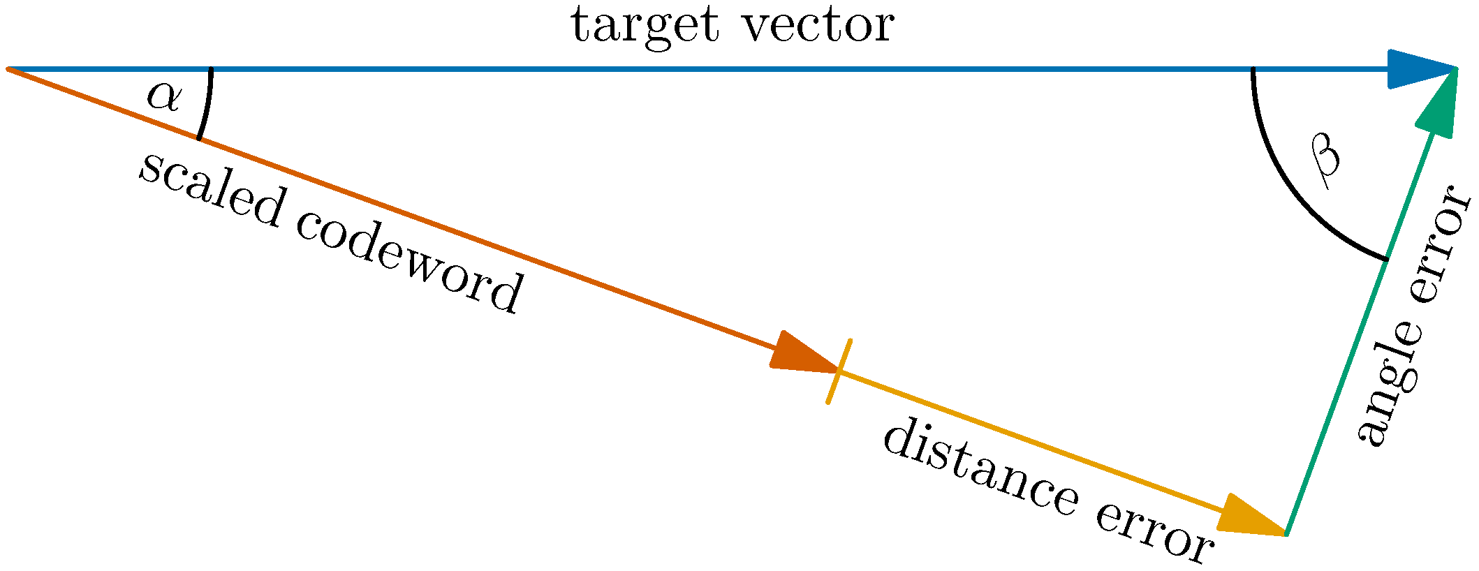
The exponential scaling of the aspect ratio is fundamental. This is a consequence of extreme-value statistics of large-dimensional random vectors: Consider the correlation coefficients (inner products normalized by their Euclidean norms) of N-dimensional real random vectors with IID entries in the limit . For any set of those vectors whose size is polynomial in N, the squared maximum of all correlation coefficients converges to zero, as [46]. Thus, the angle in Figure 1 becomes a right angle and the norm of the angle error is lower bounded by the norm of the target vector. However, for an exponentially large set of size with rate , the limit for is strictly positive and given by rate-distortion theory as [47]. The asymptotic squared relative error of approximating a target vector by an optimal real scaling of the best codeword is therefore . The residual error vector can be approximated by another vector of the exponentially large set to get the total squared error down to . Applying that procedure for s times, the (squared) error decays exponentially in s. In practice, the scale factor cannot be a real number, but must be quantized. This additional error is illustrated in Figure 1 and labeled distance error as opposed to the previously discussed angle error.
5.2. Angle Error
Consider a unit norm target vector that shall be approximated by a scaled version of one out of K codewords that are random and jointly independent. Denoting the angle between the target vector t and the codeword as , we can write (the norm of) the angle error as
The correlation coefficient between target vector t and codeword is given as
The angle error and the correlation coefficient are related by
We will study the statistical behavior of the correlation coefficient in order to learn about the minimum angle error.
Let denote the cumulative distribution function (CDF) of the squared correlation coefficient given target vector t. The target vector t follows a unitarily invariant distribution. Thus, the conditional CDF does not depend on it. In the sequel, we choose t to be the first unit vector of the coordinate system, without loss of generality.
The squared correlation coefficient is known to be distributed according to the beta distribution with shape parameters and Section III.A in [48], and given by
5.3. Distance Error
Consider the right triangle in Figure 1. The squared Euclidean norms of the angle error and the codeword scaled by the optimal factor give
for a target vector of unit norm. The distance error is maximal, if the magnitude of the optimum scale factor is exactly in the middle of two adjacent powers of two, say and . In that case, we have
which results in
Due to the orthogonal projection, the magnitude of the optimal scale factor is given as
Thus, the distance error obeys
with equality, if the optimal scale factor is three quarters of a signed power of two.
It will turn out useful to normalize the distance error as
and specify its statistics by , to avoid the statistical dependence of the angle error. The distance error is a quantization error. Those errors are commonly assumed uniformly distributed [13]. Following this assumption, the average squared distance error is easily calculated as
Unless the angle is very small, the distance error is significantly smaller than the angle error. Their averages become equal for an angle of arccot .
Note that the factor slightly differs from the factor in Example 2. Like in Example 2, the number to be quantized is uniformly distributed within some interval. Here, however, the interval boundaries are not signed powers of two. This leads to a minor increase in the power of the quantization noise.
5.4. Total Error
Since distance error and angle error are orthogonal to each other, the total squared error is simply given as
Conditioning on the normalized distance error, the total squared error is distributed as
The unconditional distribution
is simply found by marginalization.
As the columns of the codebook matrix are jointly independent, we conclude that for
we have
For having support in the vicinity of , it is shown in Appendix C to converge to
for exponential aspect ratios.
The large matrix limit (40) does not depend on the statistics of the normalized distance error. It is indifferent to the accuracy of the quantization. This looks counterintuitive and requires some explanation. To understand that effect, consider a hypothetical equiprobable binary distribution of the normalized distance error with one of the point masses at zero. If we now discard all codewords that lead to a nonzero distance error, we force the distance error to zero. On the other side, we lose half of the codewords, so the rate is reduced by . However, in the limit , that comes for free. If the distribution of the angle error has any nonzero probability accumulated in some vicinity of zero, a similar argument can be made. This above argument is not new. It is common in forward error correction coding and is known as the expurgation argument [50].
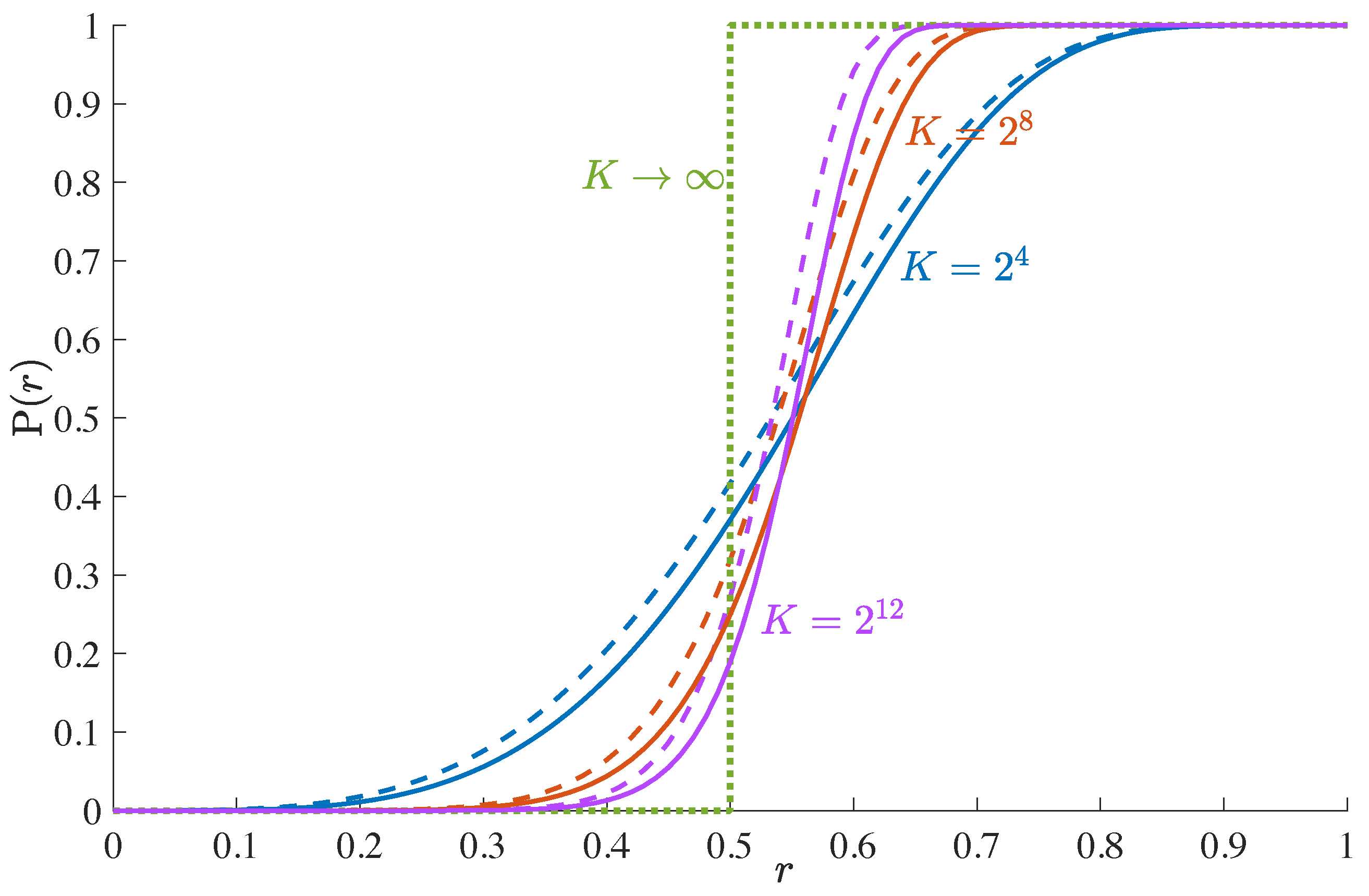
The CDF is depicted in Figure 2 for a uniform distribution of the distance error. For increasing matrix size, it approaches the unit step function. The difference between the angle error and the total error is small.
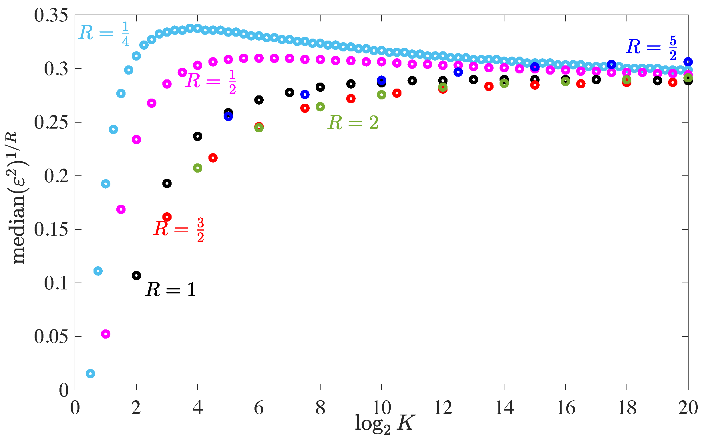
The median total squared error for a single approximation step is depicted in Figure 3 for various rates R. Note that the computational cost per matrix entry scales linearly with R for fixed K. In order to have a fair comparison, the average total squared error is exponentiated with . For large matrices, it converges to the asymptotic value of found in (40), which is approached slowly from above. For small matrices, it strongly deviates from that. While for very small matrices low rates are preferred, medium-sized matrices favor moderately high rates between 1 and 2. Having the rate too large, e.g., , also leads to degradations.
We prefer to show the median error over the average error that was used in the conference versions [4,43] of this work. The average error is strongly influenced by rare events, i.e., codebook matrices with many close to collinear columns. However, such rare bad events can be easily avoided by means of cutting diversity, cf. Section 4.4.5. The median error reflects the case that is typical, in practice.
5.5. Total Number of Additions
The exponential aspect ratio has the following impact on the trade-off between distortion and computational cost: For choices from the codebook, the wiring matrix contains nonzero signed digits according to approximation (20). Due to the columnwise decomposition, these are of them per column. At this point, we must distinguish between wide and tall matrices.
- Wide Matrices:
- For the number of additions, the number of nonzero signed digits per row is relevant, as each row of is multiplied to an input vector x when calculating the product . For the standard choice of square wiring matrices, the counting per column versus counting per row hardly makes a difference on average. Though they may vary from row to row, the total number of additions is approximately equal to .
- Tall Matrices:
- The transposition converts the columns into rows. Thus, is exactly the number of additions.
In order to approximate an target matrix with rows, we need approximately additions. For any desired distortion D, the computational cost of the product is by a factor smaller than the number of entries in the target matrix. This is the same scaling as in the mailman algorithm. Given such a scaling, the mailman algorithm allows for a fixed distortion D, which depends on the size of the target matrix. The proposed algorithm, however, can achieve arbitrarily low distortion by setting appropriately large, regardless of the matrix size.
Computations are also required for the codebook matrix. All three codebook matrices discussed in Section 4.4 require at most K and additions for tall and wide matrices, respectively. Adding the computational costs of wiring and codebook matrices, we obtain
with and
Normalizing to the number of elements of the target matrix , we have
The computational cost per matrix entry vanishes with increasing matrix size. This behavior fundamentally differs from state-of-the-art methods discussed in Examples 1 and 2, where the matrix size has no impact on the computational cost per matrix entry.
6. Simulation Results
In this section, we present simulation results to show the performance of the proposed linear computation coding in practice, compare it to competing methods from the literature, as well as test the accuracy of our analytical analysis.
6.1. Compounding
The greedy wiring approach, cf. Section 4.5, is based on compounding. Each new addition serves to reduce the total squared error by a certain factor, asymptotically by . In the analysis, we have assumed that the target vector is statistically independent of the codebook. In the greedy approach, however, the running target vector depends on the wiring of the previous matrix factor. Thus, this independence assumption is violated. The practically important question is, whether this violation has any significant effect. If so, we could not simply multiply the individual savings of each wiring matrix to get the total saving.
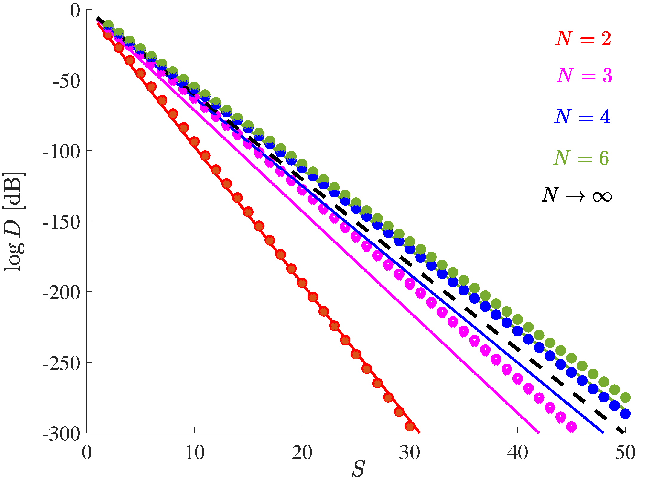
Consider L wiring matrices each with two nonzero entries per column, i.e., for all ℓ. Let denote the median of the unconditional distribution of the total squared error given in (37). The median of total distortion is shown in Figure 4 vs. S (approximately the total number of additions per column required for all wiring matrices) and compared to . For unit rate, is very close to the simulation results. The violation of the independence assumption appears to have a rather minor effect.
While for , all curves are close to each other, is exceptional. This does not imply, however, that small matrix size is beneficial. Contrarily, the number of additions per matrix entry is given in (43), which clearly decays with increasing matrix size.
The influence of the codebook in Figure 4 is very small. Only for is a difference between the mailman and the IID Gaussian codebook visible. This is partially a result of codebook evolution, as discussed in Section 4.4.4.
6.2. Codebook Comparison
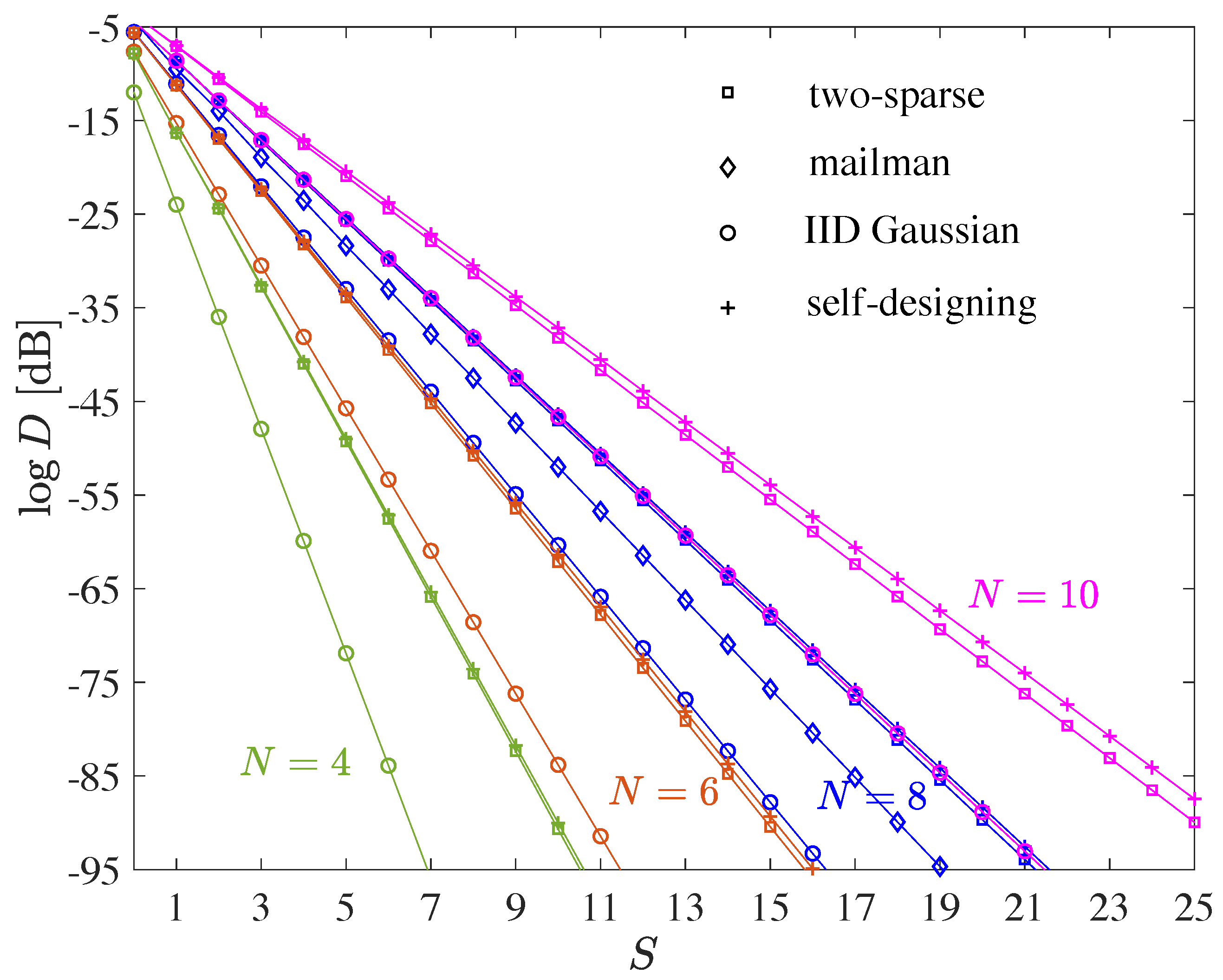
For an IID Gaussian target matrix with columns, we compare various codebook matrices in Figure 5. In contrast to Figure 1 in [43], we use a single wiring matrix to avoid the effects of codebook evolution. The wiring matrix is designed as described in Section 4.2.2.
The Gaussian codebook, of course, is not useful for practice due to its high computational cost. It is just shown as a benchmark. For all numbers of rows N that are shown in the figure, Gaussian codebooks perform significantly superior while the self-designing and two-sparse codebooks perform the worst. The mailman codebook, which only exists for , bridges half the gap to the Gaussian codebook. The choice of the codebook affects the slope of the curve.
Codebook evolution can be quite helpful to obtain a good codebook. Note that in Figure 4 there is hardly any difference between the Gaussian and the mailman codebook. This is due to codebook evolution. Whenever the target matrix is a good codebook, codebook evolution can be utilized to convert an initial poorly performing codebook into a good one. In that case, we need multiple wiring matrices.
If the target matrix is a poor codebook, we cannot utilize codebook evolution directly. However, we can invest few wiring matrices to build up the codebook Gaussian-like, before we fix the approximately Gaussian codebook and wire all the remaining computation via a single wiring matrix. The creation of a good codebook initially incurs additional computational costs, but these can be more than offset by a faster decay of the distortion.
6.3. Number of Additions Per Matrix Entry
Due to their superior performance, we use evolutionary codebooks. Since the initial codebook hardly matters in that case, we choose the self-designing codebook for the sake of simplicity and flexibility. Since the number of additions in (43) is only approximately correct for wide matrices, while it is exact for tall matrices, we study the latter in this section.
6.3.1. IID Gaussian Target Matrices
If the target matrix is IID Gaussian, it is well-suited to self-design the codebook, as IID Gaussian codebooks work excellently. As in Section 6.1, we use wiring matrices with . Table 1 shows the average number of additions per matrix entry to achieve a certain accuracy ranging from 24 dB to 144 dB SQNR. SQNRs of 24 dB, 48 dB, 72 dB, 96 dB, 120 dB, and 144 dB are commonly associated with the accuracy of 4, 8, 12, 16, 20, and 24-bit integer arithmetic, respectively. This correspondence is pretty accurate for uniformly distributed random variables. For Gaussian random variables, a few additional bits are required to achieve that accuracy, in practice, as one has to avoid clipping effects and to encode the sign.
A integer number of matrix factors clearly does not to lead to an integer multiple of 24 dB in SQNR. Therefore, we used interpolation to find the fractional number of matrix factors that are required to achieve a certain SQNR. A fractional number of matrix factors is not impossible, in practice. It simply means that the last wiring matrix contains only a single nonzero entry in some, but not all of its rows.
For higher and lower accuracies, higher and lower code rates are favored, respectively. This behavior is explained as follows: There is the fixed computational cost of about K additions for the codebook matrix. The higher the code rate, the fewer rows share this cost. This increases the computational burden per row (and also per matrix entry) for higher code rates. For high accuracy, the wiring matrices clearly dominate the computational cost, so the computation of the codebook is secondary. Thus, higher rates are favored, as they generally result in lower distortions, see Figure 3. For low accuracy, only few wiring matrices are needed, and the relative cost of the codebook is more important. This shifts the optimum rate towards lower values.
In the last two rows of Table 1, we compare linear computation coding to our benchmark set by Booth’s CSD representation, cf. Section 3. For Gaussian distributed random variables, (5) is not valid. Therefore, we obtained an equivalent relation by means of computer simulation averaging of 106 Gaussian random numbers—which turns out to be very close to (5), though—to obtain the penultimate row in the table.
CSD, however, can do better than that. Instead of using a fixed number of CSDs for each entry of the matrix, one could also adaptively assign more or less digits to the various entries, based on the overall gain in reducing the total quantization error. Such a procedure leads to the last row in Table 1 and is marked as CSDa.
The number of additions per matrix entry hardly depends on the size of the matrix, as CSD works element-wise. It reduces the effort of scalar multiplications, which are required exactly once per matrix entry. Only when it comes to summing these scalar products to obtain the output vector, does the number of columns of the matrix matter. This is, as summing N numbers only required additions. After normalization, this yields the corrections in the table.
Returning to the matrix of Examples 1 and 2, we cut this matrix into 32 tall submatrices of size . According to Table 1, we need additions for the 32 submatrix-vector products to obtain 96 dB SQNR, if the matrix has IID Gaussian entries. Furthermore, we need additions to sum the subvectors in (10). In total, that gives million additions. This means 1.557 additions per matrix entry. Note that the number of additions per matrix entry in Table 1 is 1.549 for a matrix, while we actually need 1.557 for the matrix. Apparently, the surplus effort for summing the subvectors in (10) is insignificant. For the two CSD methods, we obtain and , respectively. In comparison to these, linear computation coding requires 77% and 71% fewer additions, respectively.
6.3.2. IID Uniform Target Matrices
Consider now a random matrix whose entries are uniform IID within . If the same algorithm is used as before, the performance degrades significantly, as such a matrix is not a good codebook. Since all entries are positive, all codewords are constrained to a single orthant of the full space. A uniform distribution within , on the other hand, would hardly be an issue.
We write the target matrix as . We deal with the matrix whose entries are uniformly distributed within in exactly the same way as in Section 6.3.1. We calculate the term directly and add the result to . In addition to the linear computation coding for , this requires additions for and K additions for adding to . Since the norm of is half the norm of , the SQNR for may be 6 dB lower than for . The results are shown in Table 2. A comparison to Table 1 shows that this procedure only causes a minor degradation, if any at all, that is more pronounced for small matrices.
For comparison, Table 2 also shows the number of additions required for the CSD representation. Here, the rows CSD and CSDa refer to the same methodology as in Table 1. The last two rows indexed by an additional “h”, refer to the hybrid approach of decomposing into its mean and . This approach is not only useful for linear computation coding, but also for the CSD representation.
For the matrix of Examples 1 and 2, this time with uniform entries within , we use the same cut into 32 submatrices of size . With the results of Table 2, this results in 1.575 additions per matrix entry for 96 dB SQNR. Compared to the four variants of CSD representation shown in Table 2, this means savings of 76%, 69%, 75%, and 68%, respectively.
6.4. Competing Algorithms beyond CSD
As discussed in Section 3.1, CSD is not the most efficient method reported in literature. Various further optimizations are possible. The search for common subexpressions in the calculations has been the most successful of them so far.
6.4.1. Multiplierless Multiple Constant Multiplication
An efficient approach in the literature is reported in [29]. For a bit width of 12, which corresponds to a distortion level of dB, approximately one addition per entry is reported for multiplying a vector t with a scalar constant x Figure 12a of [29], if the dimension of the vector t is larger than 20.
When utilizing the method of [29] for matrix–vector multiplication, however, one also has to sum the vector-scalar products to obtain the final result. This requires close to one further addition per matrix entry (precisely additions). So, in total close to two additions per matrix entry are required. A comparison with Table 1 and Table 2 shows that our method is inferior for matrix sizes up to 64, but superior for matrix sizes of 256 and beyond. For matrices of size 4096, we even save about 40% of the additions. While the savings in [29] hardly depend on the size of the matrix, the efficiency of our method increases with matrix size.
The complexity of the preprocessing algorithm in [29] is much higher. As reported in Table VII in [29] it scales, even in its simplified form, as with N and b denoting vector dimension and bit width, respectively. For a square matrix containing N columns and rows, that results in an overall complexity of . Our method, by contrast, has decomposition complexity . As a result, simulating the precise performance of the algorithm in [29] for large matrices, where our method is most competitive, is practically infeasible.
6.4.2. Multiplierless Matrix-Vector Multiplication
The ideas of subexpression sharing in multiple constant multiplication are applied in several lines of work concerned with matrix-vector multiplication. Early studies have focused on structured matrices. Reference [32] is the first one to report results on unstructured matrices. For random matrices of size and 8-bit precision (corresponding to a distortion level of −48 dB) an average number of 412.4 additions is reported in Table 7 in [32]. This means 1.61 additions per matrix entry. Similar to [29], the number of required additions in [32] hardly depends on the size of the random matrix and the complexity of the preprocessing scales with the fourth power of matrix size. This means that the algorithm in [32] outperforms our algorithm in terms of number of additions for matrices. For matrix size , it already falls behind our method.
Improvements can be found in subsequent work on subexpression sharing: In Table VIII in [33] only 338.3 additions on average are reported for the same setting as above. This means 1.32 additions per matrix entry. This is better than our results for matrix size , but worse than what we achieve for matrix size . This reduced number of additions in [33] comes at a high price: The complexity of the preprocessing scales approximately with the fifth to sixth power of the matrix size, see Figure 2c in [34]. The best result for subexpression sharing we could find in the literature is due to [34]. Allowing for exponential complexity in the preprocessing, Figure 2a in [34] reports only 1.15 additions per matrix entry on average. This beats our method for size , though it is more than questionable whether the NP-complete algorithm can be implemented for that matrix size. For matrices of size or larger, our algorithm requires fewer additions.
The method in Figure 4a in [35] requires about 2.1 additions per entry for an 8-bit matrix of size . This is not competitive with the methods described above. However, the optimization goal of this paper also cares to reduce the overall delay in the signal flow which is important for pipelining in FPGAs. A problem which often occurs in subexpression sharing is as follows: Some intermediate results are ready earlier than others, thus computing units need to wait for others to finish before they can continue. This problem does not occur in our approach, if we use the vertical decomposition. In that case, all computing paths have exactly the same lengths and all computations can be pipelined.
7. Computation-Distortion Trade-Off
Combining the results of Section 5.4, Section 5.5, and Section 6.1, we can relate the mean-square distortion to the number of additions. Section 6.1 empirically confirmed that the distortion is given by
(at least for rates close to unity). Combining (40) and (21), we have
for matrices with large dimensions. Furthermore, (43) relates the number of additions per matrix entry to S and N as
Combining these three relations, we obtain
This is a much more optimistic scaling than in Example 2. For scalar linear functions, Booth’s CSD representation made the mean-square error reduce by the constant factor of 28 per addition. Due to linear computation coding as proposed in this work, the factor 28 in (5) turns into , the squared matrix dimension, in (47). Since we have the free choice to go for either tall or wide submatrices, the relevant matrix dimension here is the maximum of the number of rows and columns.
We may relate the computational cost in (47) to the computational cost in (5), the benchmark set by Booth’s CSD representation. For given SQNR, this results in
For q-bit signed integer arithmetic the SQNR is approximately given by SQNR . Thus, we obtain
Although this formula is based on asymptotic considerations, it is quite accurate for the benchmark example. Instead of the actual 77% savings compared to CSD, which were found by simulation in Section 6.3.1, it predicts savings of 79%. However, it does not allow to include adaptive assignments of CSDs.
8. Conclusions and Outlook
Linear computation coding by means of codebook and wiring matrices is a powerful tool to reduce the computational cost of matrix–vector multiplications in deep neural networks. The idea of computation coding is not restricted to linear functions. Its direct application to multidimensional nonlinear functions promises even greater reductions in the computational cost of neural networks.
The considerations in this work are limited to measure computational cost by counting additions. It is to be investigated how the savings reported in terms of additions relate to overall savings on various computer architectures. For field programmable gate arrays, very similar savings are reported in [10] counting look-up tables.
9. Patents
Concerning the method for matrix–vector multiplication proposed in this work, patent applications have been filed in 2020 and 2022.
Author Contributions
R.R.M. performed most of the work. B.M.W.G. and A.B. contributed to literature survey, paper writing, and computer simulations. All authors have read and agreed to the published version of the manuscript.
Funding
This work was partially supported by Deutsche Forschungsgemeinschaft (DFG) under grant MU-3735/8-1.
Institutional Review Board Statement
Not applicable.
Informed Consent Statement
Not applicable.
Data Availability Statement
Not applicable.
Acknowledgments
The authors like to thank Veniamin Morgenshtern, Marc Reichenbach, Hans Rosenberger, and Hermann Schulz-Baldes for helpful discussions.
Conflicts of Interest
The funders had no role in the design of the study; in the collection, analyses, or interpretation of data; in the writing of the manuscript; or in the decision to publish the results.
Appendix A. Average Distortion of Canonical Signed Digit Form
For the CSD form, the set of reconstruction values is . Let the target variable t be uniformly distributed within . Thus, only reconstruction values for are used.
Consider the interval with . The probability that the variable t falls within that interval is equal to its width . The average mean-squared quantization error within that interval is well known to be . Averaging over all intervals, the average mean-squared distortion for quantization with a single digit is given by
By symmetry, the same considerations hold true, if t is uniformly distributed within . Due to the signed digit representation, these considerations even extend to t uniformly distributed within .
For representation by zero digits, is quantized to 0 with average mean-squared distortion equal to . This is 28 times larger than for quantization with one digit.
The CSD representation is invariant to any scaling by a power of two. Thus, any further digit of representation also reduces the average mean-squared distortion by a factor of 28.
Appendix B. Additions Required for Binary Mailman Codebook
Let denote the binary mailman matrix with N rows and K columns. It can be decomposed recursively as
- Wide Matrices:
- These are additions for , additions for the matrix–vector product, and additions to sum the components of . Note that . Thus, and for .
- Tall Matrices:
- In this case, we decompose h into its first components collected in and the last component denoted by . We obtainLet denote the number of additions to compute the product . The recursion (A7), impliesThese are additions for the matrix–vector product, and additions to add . Note that . Thus, and for .
Appendix C. Asymptotic Cumulative Distribution Function
In order to show the convergence of the CDF of the squared angle error to the unit step function, recall the following limit holding for any positive x and u:
The limiting behavior of is, thus, decided by the scaling of with respect to K. The critical scaling is . Such a scaling implies a slope of in doubly logarithmic scale. Thus,
Explicit calculation of the derivative yields
with the definition
By saddle point integration, Chapter 4 in [51], we have for any function that is bounded away from zero and infinity within the open unit interval and that does not depend on N
This leads to
which immediately implies .
References
- Shen, W.W.; Lin, Y.M.; Chen, S.C.; Chang, H.H.; Lin, C.C.; Chou, Y.F.; Kwai, D.M.; Chen, K.N. 3-D Stacked Technology of DRAM-Logic Controller Using Through-Silicon Via (TSV). IEEE J. Electron Devices Soc. 2018, 6, 396–402. [Google Scholar] [CrossRef]
- Hong, S.; Auciello, O.; Wouters, D. (Eds.) Emerging Non-Volatile Memories; Springer: Berlin/Heidelberg, Germany, 2014. [Google Scholar]
- Castañeda, O.; Jacobsson, S.; Durisi, G.; Goldstein, T.; Studer, C. Finite-Alphabet MMSE Equalization for All-Digital Massive MU-MIMO mmWave Communication. IEEE J. Sel. Areas Commun. 2020, 38, 2128–2141. [Google Scholar] [CrossRef]
- Müller, R. Energy-Efficient Digital Beamforming by Means of Linear Computation Coding. In Proceedings of the 2021 IEEE Statistical Signal Processing Workshop (SSP), Rio de Janeiro, Brazil, 11–14 July 2021. [Google Scholar]
- Strassen, V. Gaussian Elimination is not Optimal. Numer. Math. 1969, 13, 354–356. [Google Scholar] [CrossRef]
- Copperfield, D.; Winograd, S. Matrix multiplication via arithmetic progressions. J. Symb. Comput. 1990, 9, 251–280. [Google Scholar]
- Han, S.; Pool, J.; Tran, J.; Dally, W. Learning both weights and connections for efficient neural network. In Proceedings of the Advances in Neural Information Processing Systems 28, Montreal, QC, Canada, 7–12 December 2015. [Google Scholar]
- Louizos, C.; Ullrich, K.; Welling, M. Bayesian compression for deep learning. In Proceedings of the 31st Conference on Neural Information Processing Systems (NIPS 2017), Long Beach, CA, USA, 4–9 December 2017. [Google Scholar]
- Evci, U.; Pedregosa, F.; Gomez, A.; Elsen, E. The Difficulty of Training Sparse Neural Networks. arXiv 2019, arXiv:1906.10732v2. [Google Scholar]
- Lehnert, A.; Holzinger, P.; Pfenning, S.; Müller, R.; Reichenbach, M. Most Resource Efficient Matrix Vector Multiplication on Reconfigurable Hardware. IEEE Access, 2022; submitted. [Google Scholar]
- Palem, K.; Lingamneni, A. Ten years of building broken chips: The physics and engineering of inexact computing. ACM Trans. Embed. Comput. Syst. 2013, 12, 87. [Google Scholar] [CrossRef]
- DeVore, R.A. Nonlinear Approximation. Acta Numer. 1998, 7, 51–150. [Google Scholar] [CrossRef] [Green Version]
- Gray, R.M.; Neuhoff, D.L. Quantization. IEEE Trans. Inf. Theory 1998, 44, 2325–2383. [Google Scholar] [CrossRef]
- Booth, A.D. A signed binary multiplication technique. Q. J. Mech. Appl. Math. 1951, 4, 236–240. [Google Scholar] [CrossRef]
- Karatsuba, A.; Ofman, Y. Multiplication of multidigit numbers on automata. Dokl. Akad. Nauk SSSR 1962, 145, 293–294. (In Russian) [Google Scholar]
- Toom, A.L. The complexity of a scheme of functional elements simulating the multiplication of integers. Dokl. Akad. Nauk SSSR 1963, 150, 496–498. (In Russian) [Google Scholar]
- Cook, S.A.; Aanderaa, S.O. On the Minimum Computation Time of Functions. Trans. Am. Math. Soc. 1969, 142, 291–314. [Google Scholar] [CrossRef]
- Schönhage, A.; Strassen, V. Schnelle Multiplikation großer Zahlen. Computing 1971, 7, 281–292. [Google Scholar] [CrossRef]
- Fürer, M. Faster integer multiplication. SIAM J. Comput. 2009, 39, 979–1005. [Google Scholar] [CrossRef]
- Harvey, D.; van der Hoeven, J.; Lecerf, G. Even faster integer multiplication. J. Complex. 2016, 36, 1–30. [Google Scholar] [CrossRef] [Green Version]
- Arnold, M.G.; Bailey, T.A.; Cowles, J.R.; Cupal, J.J. Redundant Logarithmic Arithmetic. IEEE Trans. Comput. 1990, 39, 1077–1086. [Google Scholar] [CrossRef]
- Huang, H.; Itoh, M.; Yatagai, T. Modified signed-digit arithmetic based on redundant bit representation. Appl. Opt. 1994, 33, 6146–6156. [Google Scholar] [CrossRef]
- Dempster, A.G.; Macleod, M.D. Use of Minimum-Adder Multiplier Blocks in FIR Digital Filters. IEEE Trans. Circuits Syst.-II Analog Digit. Signal Process. 1995, 42, 569–577. [Google Scholar] [CrossRef]
- Hartley, R.I. Subexpression sharing in filters using canonic signed digit multipliers. IEEE Trans. Circuits Syst.-II Analog Digit. Signal Process. 1996, 43, 677–688. [Google Scholar] [CrossRef]
- Lefèvre, V. Moyens Arithmétiques Pour Un Calcul Fiable. Ph.D. Thesis, École Normale Supérieure de Lyon, Lyon, France, 2000. [Google Scholar]
- Cappello, P.R.; Steiglitz, K. Some Complexity Issues in Digital Signal Processing. IEEE Trans. Acoust. Speech Signal Process. 1984, ASSP-32, 1037–1041. [Google Scholar] [CrossRef] [Green Version]
- Dimitrov, V.S.; Jullien, G.A.; Miller, W.C. Theory and applications of the double-base number system. IEEE Trans. Comput. 1999, 48, 1098–1106. [Google Scholar] [CrossRef]
- Dimitrov, V.S.; Järvinen, K.U.; Adikari, J. Area-efficient multipliers based on multiple-radix representations. IEEE Trans. Comput. 2011, 60, 189–201. [Google Scholar] [CrossRef]
- Voronenko, Y.; Püschel, M. Multiplierless multiple constant multiplication. ACM Trans. Algorithms 2007, 3, 11–48. [Google Scholar] [CrossRef]
- de Dinechin, F.; Filip, S.I.; Forget, L.; Kumm, M. Table-Based versus Shift-And-Add constant multipliers for FPGAs. In Proceedings of the IEEE 26th Symposium on Computer Arithmetic (ARITH), Kyoto, Japan, 10–12 June 2019. [Google Scholar]
- Cooley, J.W.; Tukey, J.W. An algorithm for the machine calculation of complex Fourier series. Math. Comput. 1965, 19, 291–301. [Google Scholar] [CrossRef]
- Boullis, N.; Tisserand, A. Some Optimizations of Hardware Multiplication by Constant Matrices. IEEE Trans. Comput. 2005, 54, 1271–1282. [Google Scholar] [CrossRef]
- Aksoy, L.; Costa, E.; Flores, P.; Monteiro, J. Optimization Algorithms for the Multiplierless Realization of Linear Transforms. ACM Trans. Des. Autom. Electron. Syst. 2012, 17, 3. [Google Scholar] [CrossRef]
- Aksoy, L.; Flores, P.; Monteiro, J. A novel method for the approximation of multiplierless constant matrix vector multiplication. EURASIP J. Embed. Syst. 2016, 2016, 12. [Google Scholar] [CrossRef] [Green Version]
- Kumm, M.; Hardieck, M.; Zipf, P. Optimization of Constant Matrix Multiplication with Low Power and High Throughput. IEEE Trans. Comput. 2017, 66, 2072–2080. [Google Scholar] [CrossRef]
- Gustafsson, O. Lower Bounds for Constant Multiplication Problems. IEEE Trans. Circuits Syst.-II Express Briefs 2007, 54, 974–978. [Google Scholar] [CrossRef]
- Volder, J.E. The CORDIC Trigonometric Computing Technique. IRE Trans. Electron. Comput. 1959, EC-8, 330–334. [Google Scholar] [CrossRef]
- Liberty, E.; Zucker, S.W. The Mailman algorithm: A note on matrix-vector multiplication. Inf. Process. Lett. 2009, 109, 179–182. [Google Scholar] [CrossRef] [Green Version]
- Kronrod, M.A.; Arlazarov, V.L.; Dinic, E.A.; Faradzev, I.A. On economic construction of the transitive closure of a direct graph. Dokl. Akad. Nauk SSSR 1970, 194, 487–488. (In Russian) [Google Scholar]
- Williams, R. Matrix-Vector Multiplication in Sub-Quadratic Time (Some Preprocessing Required). In Proceedings of the Eighteenth Annual ACM-SIAM Symposium on Discrete Algorithms; Society for Industrial and Applied Mathematics, New Orleans, LA, USA, 7–9 January 2007; pp. 995–1001. [Google Scholar]
- Merhav, N. Multiplication-Free Approximate Algorithms for Compressed-Domain Linear Operations on Images. IEEE Trans. Image Process. 1999, 8, 247–254. [Google Scholar] [CrossRef] [PubMed] [Green Version]
- Müller, R.; Gäde, B.; Bereyhi, A. Efficient Matrix Multiplication: The Sparse Power-of-2 Factorization. In Proceedings of the Information Theory & Applications Workshop, San Diego, CA, USA, 2–7 February 2020. [Google Scholar]
- Müller, R.; Gäde, B.; Bereyhi, A. Linear Computation Coding. In Proceedings of the IEEE International Conference on Acoustics, Speech and Signal Processing (ICASSP), Toronto, ON, Canada, 6–11 June 2021. [Google Scholar]
- Mallat, S.G.; Zhang, Z. Matching Pursuit with Time-Frequency Dictionaries. IEEE Trans. Signal Process. 1993, 41, 3397–3415. [Google Scholar] [CrossRef] [Green Version]
- Pati, Y.C.; Rezaiifar, R.; Krishnaprasad, P.S. Orthogonal Matching Pursuit: Recursive Function Approximation with Applications to Wavelet Decomposition. In Proceedings of the 27th Asilomar Conference on Signals, Systems and Computers, Pacific Grove, CA, USA, 1–3 November 1993. [Google Scholar]
- Jiang, T. The asymptotic distribution of the largest entries of sample correlation matrices. Ann. Appl. Probab. 2004, 14, 865–880. [Google Scholar] [CrossRef] [Green Version]
- Berger, T. Rate Distortion Theory; Prentice-Hall: Eaglewood Cliffs, NJ, USA, 1971. [Google Scholar]
- Müller, R. On Approximation, Bounding & Exact Calculation of Block Error Probability for Random Code Ensembles. IEEE Trans. Commun. 2021, 69, 2987–2996. [Google Scholar]
- Spanier, J.; Oldham, K.B. An Atlas of Functions; Springer: Berlin, Germany, 1987. [Google Scholar]
- MacKay, D.J. Information Theory, Inference, and Learning Algorithms; Cambridge University Press: Cambridge, UK, 2003. [Google Scholar]
- Merhav, N. Statistical physics and information theory. Found. Trends Commun. Inf. Theory 2010, 6, 1–212. [Google Scholar] [CrossRef] [Green Version]
Figure 1.
Decomposition of the approximation error.

Figure 2.
CDF of the squared total error (solid lines) and squared angle error (dashed lines) for rate and various numbers of columns K.
Figure 2.
CDF of the squared total error (solid lines) and squared angle error (dashed lines) for rate and various numbers of columns K.

Figure 3.
Rth root of median total squared error vs. the number of columns K in logarithmic scale for various rates R.
Figure 3.
Rth root of median total squared error vs. the number of columns K in logarithmic scale for various rates R.

Figure 4.
Median total squared error D for target matrix of unit Frobenius norm vs. the parameter S (approximately the total number of additions per column required for all wiring matrices). The solid lines refer to , the markers to simulation results. Circles and crosses are for IID Gaussian codebook matrices and mailman codebooks, respectively, all with unit rate. IID Gaussian target matrices. Results are averaged over 106 random matrix entries.

Figure 5.
Median total squared error D for target matrix of unit Frobenius norm vs. the parameter S (approximately the total number of additions per column required for all wiring matrices). Gaussian IID target matrices of size . Results are averaged over 106 random matrix entries.
Figure 5.
Median total squared error D for target matrix of unit Frobenius norm vs. the parameter S (approximately the total number of additions per column required for all wiring matrices). Gaussian IID target matrices of size . Results are averaged over 106 random matrix entries.


Table 1.
Average number of additions per matrix entry that are required to have the median distortion a certain level (between 24 and 144 dB) below the norm of the output vector. Best values for given matrix width are shown in boldface.
Table 1.
Average number of additions per matrix entry that are required to have the median distortion a certain level (between 24 and 144 dB) below the norm of the output vector. Best values for given matrix width are shown in boldface.
| dB | dB | dB | dB | dB | dB | |
| 0.948 | 2.243 | 3.490 | 4.715 | 5.922 | 7.124 | |
| 0.819 | 1.650 | 2.465 | 3.273 | 4.075 | 4.872 | |
| 0.874 | 1.793 | 2.699 | 3.597 | 4.493 | 5.384 | |
| 0.787 | 1.438 | 2.036 | 2.630 | 3.222 | 3.813 | |
| 0.756 | 1.390 | 2.020 | 2.651 | 3.278 | 3.906 | |
| 0.725 | 1.389 | 2.053 | 2.713 | 3.374 | 4.032 | |
| 0.726 | 1.425 | 2.123 | 2.817 | 3.510 | 4.203 | |
| 0.786 | 1.341 | 1.808 | 2.272 | 2.734 | 3.196 | |
| 0.729 | 1.217 | 1.702 | 2.187 | 2.671 | 3.155 | |
| 0.662 | 1.164 | 1.665 | 2.165 | 2.664 | 3.163 | |
| 0.631 | 1.144 | 1.657 | 2.169 | 2.682 | 3.196 | |
| 0.615 | 1.140 | 1.665 | 2.190 | 2.714 | 3.240 | |
| 0.606 | 1.143 | 1.679 | 2.216 | 2.751 | 3.286 | |
| 0.602 | 1.150 | 1.697 | 2.244 | 2.792 | 3.338 | |
| 0.601 | 1.159 | 1.717 | 2.274 | 2.832 | 3.389 | |
| 0.602 | 1.171 | 1.740 | 2.308 | 2.876 | 3.447 | |
| 0.633 | 1.040 | 1.442 | 1.844 | 2.246 | 2.648 | |
| 0.589 | 1.000 | 1.409 | 1.819 | 2.229 | 2.639 | |
| 0.560 | 0.977 | 1.394 | 1.811 | 2.228 | 2.645 | |
| 0.541 | 0.964 | 1.386 | 1.809 | 2.232 | 2.655 | |
| 0.528 | 0.956 | 1.384 | 1.812 | 2.241 | 2.668 | |
| 0.519 | 0.952 | 1.385 | 1.818 | 2.251 | 2.683 | |
| 0.513 | 0.951 | 1.388 | 1.825 | 2.263 | 2.700 | |
| 0.505 | 0.951 | 1.398 | 1.844 | 2.290 | 2.736 | |
| 0.503 | 0.953 | 1.402 | 1.852 | 2.301 | 2.752 | |
| 0.499 | 0.960 | 1.422 | 1.884 | 2.344 | 2.806 | |
| 0.498 | 0.964 | 1.429 | 1.894 | 2.359 | 2.824 | |
| 0.498 | 0.971 | 1.443 | 1.916 | 2.389 | 2.860 | |
| 0.499 | 0.974 | 1.450 | 1.926 | 2.402 | 2.878 | |
| 0.505 | 0.856 | 1.206 | 1.555 | 1.905 | 2.255 | |
| 0.486 | 0.840 | 1.193 | 1.547 | 1.901 | 2.254 | |
| 0.472 | 0.829 | 1.186 | 1.543 | 1.899 | 2.256 | |
| 0.462 | 0.822 | 1.181 | 1.541 | 1.901 | 2.261 | |
| 0.454 | 0.816 | 1.179 | 1.540 | 1.903 | 2.265 | |
| 0.448 | 0.813 | 1.177 | 1.541 | 1.905 | 2.270 | |
| 0.443 | 0.810 | 1.177 | 1.543 | 1.910 | 2.276 | |
| 0.439 | 0.807 | 1.176 | 1.545 | 1.913 | 2.282 | |
| 0.435 | 0.806 | 1.176 | 1.547 | 1.918 | 2.289 | |
| 0.432 | 0.805 | 1.177 | 1.549 | 1.922 | 2.295 | |
| 0.429 | 0.804 | 1.178 | 1.553 | 1.927 | 2.302 | |
| 0.427 | 0.803 | 1.180 | 1.556 | 1.933 | 2.308 | |
| 0.425 | 0.803 | 1.181 | 1.559 | 1.938 | 2.316 | |
| 0.424 | 0.804 | 1.183 | 1.563 | 1.943 | 2.323 | |
| 0.418 | 0.809 | 1.199 | 1.590 | 1.981 | 2.373 | |
| 0.417 | 0.810 | 1.202 | 1.595 | 1.987 | 2.379 | |
| 0.417 | 0.815 | 1.213 | 1.612 | 2.009 | 2.408 | |
| 0.418 | 0.817 | 1.217 | 1.617 | 2.016 | 2.416 | |
| CSD | ||||||
| CSDa |
Table 2.
Average number of additions per matrix entry that are required to have the median distortion a certain level (between 24 and 144 dB) below the norm of the output vector.
Table 2.
Average number of additions per matrix entry that are required to have the median distortion a certain level (between 24 and 144 dB) below the norm of the output vector.
| dB | dB | dB | dB | dB | dB | |
| 1.280 | 2.578 | 3.836 | 5.069 | 6.289 | 7.493 | |
| 1.142 | 1.997 | 2.822 | 3.640 | 4.451 | 5.259 | |
| 0.846 | 1.520 | 2.196 | 2.870 | 3.541 | 4.212 | |
| 0.685 | 1.221 | 1.761 | 2.300 | 2.839 | 3.378 | |
| 0.528 | 0.975 | 1.424 | 1.873 | 2.322 | 2.771 | |
| 0.422 | 0.803 | 1.185 | 1.567 | 1.949 | 2.332 | |
| CSD | ||||||
| CSDa | ||||||
| CSDh | 1.24 + | 2.90 + | 4.56 + | 6.22 + | 7.88 + | 9.54 + |
| CSDah | 1.00 + | 2.15 + | 3.51 + | 4.86 + | 6.18 + | 7.50 + |
Publisher’s Note: MDPI stays neutral with regard to jurisdictional claims in published maps and institutional affiliations. |
© 2022 by the authors. Licensee MDPI, Basel, Switzerland. This article is an open access article distributed under the terms and conditions of the Creative Commons Attribution (CC BY) license (https://creativecommons.org/licenses/by/4.0/).
Share and Cite
MDPI and ACS Style
Müller, R.R.; Gäde, B.M.W.; Bereyhi, A. Linear Computation Coding: A Framework for Joint Quantization and Computing. Algorithms 2022, 15, 253. https://doi.org/10.3390/a15070253
AMA Style
Müller RR, Gäde BMW, Bereyhi A. Linear Computation Coding: A Framework for Joint Quantization and Computing. Algorithms. 2022; 15(7):253. https://doi.org/10.3390/a15070253
Chicago/Turabian StyleMüller, Ralf Reiner, Bernhard Martin Wilhelm Gäde, and Ali Bereyhi. 2022. "Linear Computation Coding: A Framework for Joint Quantization and Computing" Algorithms 15, no. 7: 253. https://doi.org/10.3390/a15070253
Note that from the first issue of 2016, this journal uses article numbers instead of page numbers. See further details here.