
Partitioning of Transportation Networks by Efficient Evolutionary Clustering and Density Peaks


1
LISIC, University of Littoral Côte d’Opale (ULCO), Calais, BP 719, CEDEX, 62228 Calais, France
2
LaRRIS, Faculty of Sciences, Lebanese University, Fanar, Jdeidet BP 90656, Lebanon
3
ERIC, Université de Lyon, Université de Lyon 2, ERIC UR 3083 5 Avenue Pierre Mendès France, CEDEX, F69676 Bron, France
*
Author to whom correspondence should be addressed.
Algorithms 2022, 15(3), 76; https://doi.org/10.3390/a15030076
Submission received: 20 January 2022
/
Revised: 10 February 2022
/
Accepted: 15 February 2022
/
Published: 24 February 2022
(This article belongs to the Special Issue Nature-Inspired Algorithms in Machine Learning)
Abstract
:Road traffic congestion has became a major problem in most countries because it affects sustainable mobility. Partitioning a transport network into homogeneous areas can be very useful for monitoring traffic as congestion is spatially correlated in adjacent roads, and it propagates at different speeds as a function of time. Spectral clustering has been successfully applied for the partitioning of transportation networks based on the spatial characteristics of congestion at a specific time. However, this type of classification is not suitable for data that change over time. Evolutionary spectral clustering represents a state-of-the-art algorithm for grouping objects evolving over time. However, the disadvantages of this algorithm are the cubic time complexity and the high memory demand, which make it insufficient to handle a large number of data sets. In this paper, we propose an efficient evolutionary spectral clustering algorithm that solves the drawbacks of evolutionary spectral clustering by reducing the size of the eigenvalue problem. This algorithm is applied in a dynamic environment to partition a transportation network into connected homogeneous regions that evolve with time. The number of clusters is selected automatically by using a density peak algorithm adopted for the classification of traffic congestion based on the sparse snake similarity matrix. Experiments on the real network of Amsterdam city demonstrate the superiority of the proposed algorithm in robustness and effectiveness.
1. Introduction
Most densely populated cities endure road traffic congestion. Traffic congestion causes major problems, such as time delays, air pollution, fuel consumption and accident risks, which are usually caused by the fact that road capacity cannot meet the increasing traffic demand. Traffic congestion is caused by unplanned roads, the dense volume of vehicles and the presence of critical congestion areas. In unplanned roads, transportation departments do not handle traffic closures due to extreme weather conditions and other unforeseen events.
Recently, congestion problems have increased due to the growth in population and the different changes in population density. At present, the traffic system has become a very complex problem because traffic changes are uncertain [1]. Therefore, it is difficult to obtain high-precision characterization using a standard knowledge model.
Many conventional methods have been developed to solve the problem of traffic congestion, such as urban decentralization, which can be difficult to enforce in practice [2], and urban planning, which takes into consideration the increasing number of cars in cities before building their infrastructure [3]. However, these methods can be costly considering the limited land resources.
One can use applications that consider only the present congestion situations on suggested roads to navigate within cities. However, few of these applications reroute users according to real-time traffic congestion as the trip progresses [4,5]. Hence, systems and algorithms must be designed in such a way that people can avoid traffic congestion in real time. In addition, other recent studies have attempted to predict traffic congestion in cities. A more specific approach for tackling the problem of linking traffic jams is the partitioning of the links according to traffic congestion in order to devise control strategies for solving this problem. Partitioning a network of roads into homogeneous groups can be extremely useful for traffic control considering that the congestion is spatially correlated in adjacent roads and that it propagates with different speeds [6].
In [7], the authors designed a network partition method by using the normalized cut. This method was further adapted and improved, where the authors developed a method based on the definition of the snake similarity matrix and application of the normalized cut algorithm in order to detect directional congestion within clusters and improve the performance of low connectivity networks [8].
Previous work on trajectory data clustering has mainly focused on the case where objects move freely in Euclidean space [9,10]. However, these approaches failed to account for an underlying network that constrains movement. However, network constraints play a crucial role in determining the similarity measure between the trajectories to be clustered.
Another method was proposed in which the authors elaborated an approach based on discovering the clusters of trajectories by grouping similar trajectories that visited the same links of the network [11]. Then, they extended their work to the case of links, where they grouped the common links that were visited by a large number of trajectories [12]. Therefore, the community-detection algorithm used in the clustering step of their proposed framework can be sensitive to the presence of noise, which can degrade the quality of clusters.
However, these methods cannot be directly applied to dynamic frameworks. In order to study the feasibility of the control strategy to improve the transportation networks’ performance, in this paper, we focus on the clustering of transportation networks into homogeneous traffic partitions that evolve over time [13]. Data are essential to the planning and management of issues related to transportation networks. Instead of relying on conventional models, transportation research is increasingly data-driven. With the growing quantity and quality of data being collected from intelligent transportation systems, data-driven transportation research relies on new generation techniques to analyze these data.
Recently, data-driven innovation in transportation science follows two main approaches: the technology-oriented approach to enhance the data resources available to the platform [14] and the methodology-oriented approach to improve the software part of the platform [15]. Exploratory data analysis is a heuristic search technique for finding significant relationships between variables in large data sets. Its efficiency is key to deriving insights from big data. It is the first technique when approaching the data. Exploratory data analysis has the objective of identifying attributes in a data set, using univariate data analysis to characterize the data, detecting and minimizing the impact of missing and aberrant values, detecting errors and, finally, combining features to generate new features [16].
In our case, to perform network partitioning, both the network topology and the link speeds for all time periods are needed. Therefore, data preparation is needed to create a validated data set for evolutionary spectral clustering. Data preparation aims to remove travel time outliers and coarsen the large-scale network in order to improve the computation time and to estimate link speeds. The data are gathered from the Amsterdam transportation network. The network topology is derived from both cameras and geographic information systems. An algorithm was developed to compute missing data [17].
Spectral clustering has been successfully applied to the clustering of transportation networks based on the spatial features of congestion at specific times [7,8,17]. Previous works have proposed a simple approach to this type of problem that consists of performing static clustering at each time step using only the most recent data. The main drawback of this approach is that it does not explicitly take into account the temporal aspects of traffic states.
Evolutionary spectral clustering represents algorithms for grouping objects evolving over time. It outperforms traditional static clustering by producing clustering results that can adapt to data drifts while being robust to short-term noise. According to [18], in the context of evolutionary spectral clustering, a good clustering result should fit the current data well while simultaneously not deviating too dramatically from the recent history.
In our previous work, we applied the evolutionary spectral clustering algorithm in order to partition a road network between congested and fluid zones [19]. However, the major drawback of this algorithm is the cubic time complexity and the high memory demand for computing the Laplacian matrix that makes it insufficient to handle data sets characterized by a large number of patterns.
This paper proposes an efficient evolutionary spectral clustering algorithm that provides a solution to this problem. The proposed algorithm introduces the notion of a smoothed Laplacian matrix with a weighted sum of current and past similarity matrices to efficiently solve the eigenvalue problem by means of the incomplete Cholesky decomposition. It is also equipped with a stopping criterion based on the convergence of the cluster assignments after the selection of each pivot in place of the classical stopping condition based on the low-rank assumption. In order to improve the network’s performance, the similarity matrix is computed in a way to put more weights on neighboring links and to facilitate the connectivity of the clusters.
The similarity, in this case, will be a sparse matrix, as some links have zero similarity, which can simplify the complexity of the clustering algorithm [8]. Determining the number of clusters in a data set is a frequent problem in data clustering. Choosing the appropriate number of clusters is often ambiguous, with interpretations depending on the shape and scale of the distribution of points in a data set. Many measurements have been developed for finding the optimal number of clusters. In early research, the authors proposed an algorithm to estimate the optimal number of clusters in categorical data clustering by a silhouette coefficient, which is a useful technique for assessing the number of clusters [20,21].
The silhouette of data is a measure of how closely it is matched to data within its cluster and how loosely it is matched to data of the neighboring cluster. A silhouette close to 1 implies the datum is in an appropriate cluster, whereas a silhouette close to -1 implies the datum is in the wrong cluster. However, a silhouette only reveals the quality of data in some specific set, and it does not work well in ring-shaped data sets. The gap statistic method is another method used for detecting the number of clusters. The key idea of the gap method is to compare within-cluster dispersion in the observed data to the expected within-cluster dispersion. The gap method performs well assuming that the data come from an appropriate distribution [22].
In order to identify the correct number of clusters to return from a hierarchical clustering, an efficient algorithm was developed. This algorithm makes use of the same evaluation function that is used by a hierarchical algorithm during clustering to construct an evaluation graph where the x-axis is the number of clusters, and the y-axis is the value of the evaluation function at x clusters. The point of the maximum curvature of this graph is used as the number of clusters to return. This point is determined by finding the area between the two lines that most closely fit the curve [23]. However, this method works poorly with mixed data types, and it does not work well on very large data sets.
In this paper, we introduce the density peaks algorithm, which has the ability to recognize clusters regardless of their shape. The clustering is performed using the efficient evolutionary spectral clustering algorithm, and we adapted the density peaks clustering algorithm to automatically find the number of clusters, which dynamically changes over time.
This algorithm is based on the assumptions that the cluster centers are surrounded by neighbors with a lower local density and that they also have relatively large distances from other data points with a higher local density. It also has the advantage of visualizing the structure of the data in the decision graph. The proposed algorithm is compared with the modularity and the eigengap methods to show its effectiveness.
The new contributions of this paper are summarized as follows:
- We optimize the efficient evolutionary spectral clustering algorithm in order to cluster real world traffic data sets collected from the transportation network of Amsterdam city [17]. This algorithm was built in order to handle traffic evolving over time.
- We extend this algorithm for the preserving cluster membership framework by computing a new sparse similarity matrix that considers traffic at previous times. We show that this algorithm minimizes time and space complexities. We prove that the proposed efficient evolutionary spectral clustering algorithm provides more robustness and effectiveness compared with other static clustering methods in the case of a transportation network.
- We compute the number of clusters for each time period using the density peak algorithm. We modify this algorithm in order to compute the distance between snakes based on the sparse snake similarity matrix. This algorithm is proven to be more effective than the modularity and the eigengap methods in the case of efficient evolutionary spectral clustering.
- We convert the transportation network into different graph models in order to find directional congestion. We study the evolution of the graph over different time periods of the day. We prove which clustering method is the most efficient for clustering all time-dependent road speed observations into 3D speed maps, and we study the computational times to partition the road network.
The paper is structured as follows: in Section 2, we present the graph models and how to compute the similarity matrix. We also introduce the spectral clustering algorithm ans the evolutionary spectral clustering algorithm, and we propose an efficient evolutionary spectral clustering algorithm for the partitioning of a transportation network. In Section 3, we explain how to automatically find the number of clusters using the density peak algorithm. Section 4 shows the experimental results, and finally the paper is summarized with our conclusions in Section 5.
2. Methodology
Traffic data change quickly; hence, static spectral clustering algorithms are unable to deal with data where the characteristics of link speeds to be clustered change over time. We are interested in developing a methodology based on evolutionary spectral clustering to dynamically partition a graph-based traffic network into connected and homogeneous clusters. First, we define the network of links and how to convert it into a graph of links. Next, we convert the graph of links into a graph of snakes, and then we compute the similarity matrix between snakes in order to apply clustering algorithms.
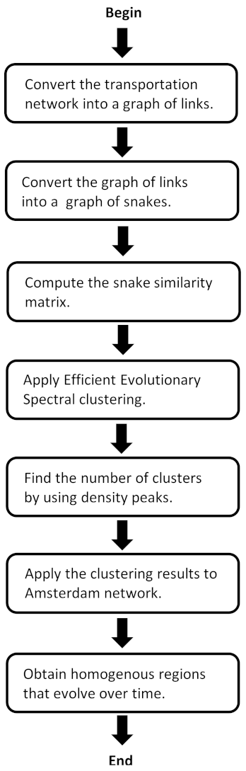
Next, we briefly explain the spectral clustering algorithm. We also introduce the evolutionary spectral clustering framework through normalized cuts and finally we give the efficient evolutionary spectral clustering algorithm in order to minimize the time and space complexities. Figure 1 shows the data flow chart (DFC) that describes our methodological steps, and Glossary shows a summary of notation symbols used in the paper.
2.1. Graph Models
This section defines the structure of the network of links and explains how to convert it into a graph of links and a graph of snakes in order to apply the spectral clustering algorithm.
2.1.1. Network of Links
A network of links is defined as comprising a set of intersection points that are connected by a set of links , where for each link , a speed value is assigned to it. Given the network of roads, we are now able to convert it into a graph of links.
2.1.2. Graph of Links
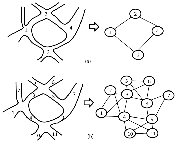
We distinguish two possible representations in order to convert the network of links into a graph of links, which are the primal graph and the dual graph (Figure 2). In the first representation, the primal graph is constructed by considering each intersection in the network as a node and adding an edge or link between each pair of nodes if there is at least one link connecting them.
In this representation, we maintain the same shape of the network of links; the edges in the graph follow the paths of the real network of links. In the second representation, the dual graph is constructed by considering each link in the network as a node and by establishing an edge between each pair of possible nodes if there is at least one common intersection between them.
In this paper, we use the primal graph, and we model the data of a network of links as a graph in which V and E are the sets of nodes and links, respectively. Two links are spatially connected if either the end or the beginning of them are connected to the same intersection. Based on this definition, all the links entering or exiting the same intersection are assumed to be connected. Moreover, links connecting to the same intersection are considered adjacent. In order to partition the graph edges into connected homogeneous traffic states, we begin to build a graph of snakes.
2.1.3. Graph of Snakes
The graph of snakes is represented as a undirected graph . The set of vertices , where represents the number of network snakes, and the set of edges represents the similarity between snakes. Although there is a one-to-one association between links and snakes, the same name is used for both the links and snakes. The value of N is computed after coarsening the large-scale transportation network of Amsterdam and removing travel time outliers [17]. A snake is formed as a concatenation of a number L of adjacent links with similar speeds. Each snake is defined in an iterative process starting from an individual link in the graph.
A snake is defined by , where , is the size of the snake, is the link composed from an identifier and a link speed , and and are connected links. The connected clusters’ dissimilarity is used to evaluate the performance of the clustering algorithm for different values of L [17].
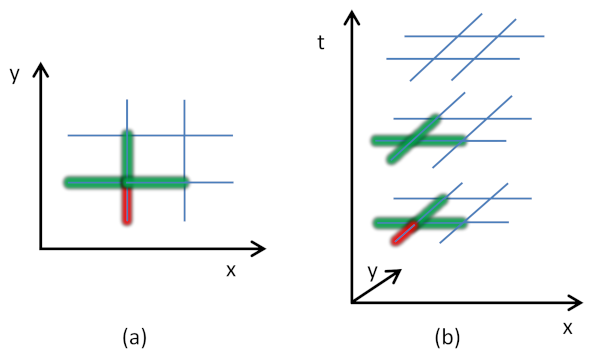
For each of the links, we iteratively build a snake, which is a sequence of links, with the objective of having a minimum variance of all the chosen link speeds at each step. One can consider this as a snake that starts from a link and grows by attracting the most similar adjacent link iteratively (Figure 3). Figure 3 shows an example of a snake, initialized by a link in red. The green links represent the neighborhood, according to two- and three-dimensional approaches.
Note that, at each step, the most similar link to the snake is the adjacent link with the closest speed value to the average speed values of the links in the snake. This procedure identifies interesting patterns as the variance grows with the size of the links. This observation is related to the fact that some parts of the graph are more similar than others, and if a large number of dissimilar links are added, high variance is unavoidable.
Thus, in each step, each snake identifies all the adjacent links and adds the one that has the smallest variance value to the average value of previously added links in that snake. This procedure continues until the snake encompasses all the links in the network. The variance value of the snake at each step l can be computed by:
where
where denotes the mean speed of the snake at each step l, and is the speed of the link added in the l-th step.
Clustering the snakes of links requires the construction of a weighted graph that encodes the similarity between data snakes. In the next section, we will explain how to build the snake similarity matrix.
2.2. Similarity
There are many proposed methods in the literature to construct a similarity matrix for a graph, such as the inner product of feature vectors, the Gaussian similarity and the cosine similarity [25]. In our study, the goal is to define a similarity between each pair of links in the network that takes into account both homogeneity and spatial connectivity. Using this similarity measure, a fully connected graph is built in which one edge exists between every two nodes, meaning that every two snakes in the network are similar.
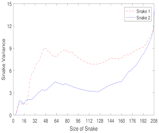
The sequence of the links in a snake not only represents the links with the close speed values but also has some information about the spatial connectivity of the links. As the size of the snake grows, this measure of similarity gives less forget weight on the links that are collected. After some iterations, the snake does not have any good options to add and starts adding links with variant speeds leading to a higher variance.
To further investigate, we plot the variance of the first and the second snake of the network of links (Figure 4). Based on these properties of the snake, we propose to put more weights on the links that are spatially closer to each other, and their corresponding snakes will converge to the same point [17].
In this case, we obtain a sparse similarity matrix. The snake similarity is defined as follows:
Note that:
where and are l-size snakes corresponding to starting links i and j, and is the number of common link identifiers between the two snakes of size l. The weight coefficient is assigned by the user with . The snake similarity matrix algorithm for the transportation network is given by Algorithm 1.
| Algorithm 1 Snake Similarity Matrix Algorithm for the Transportation Network |
|
In order to prove the correctness of the algorithm, we consider a graph of links with a certain number of homogeneous regions with different levels of congestion in the graph. The links of one region have the same density or speed value. Each snake adds the adjacent link with the closest speed value to the average speed values of the links in the snake. Snakes start from different links in each of these regions. They first integrate all the links in that region and then start adding from other regions with different levels of congestion.
We can conclude, that after reaching this state, all the snakes within one component will show the same behavior. Moreover, they have many common links during their evolution before reaching the whole component. We use these features to define a similarity matrix constituted by the number of common link identifiers between the pairs of snakes. Snakes with different initial links have a robust trend inside each cluster and converge to the same state before adding links from other clusters.
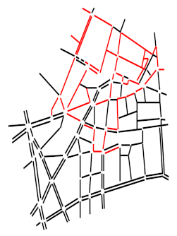
By running the snake algorithm through the graph from different links, the homogeneous regions are identified. The homogeneous regions in the graph refer to the set of links in which all snakes—starting from any initial link in that component—will end having the same links in that sequence [8]. Figure 5 shows a snake computed on the network of the sixth district of Paris.
2.3. Spectral Clustering
In graph theory, there are many clustering algorithms that assign objects into clusters with respect to their pairwise similarity measure. The success of spectral clustering is based on the fact that it does not make any assumptions about the data structure. Spectral clustering can handle complex and unknown cluster shapes; in these cases, the commonly used methods, such as K-means or mixture models, may fail.
The idea of spectral clustering is to cluster based on the eigenvectors of a similarity matrix W defined on the set of nodes of a graph in which is the set of nodes, N is the number of nodes in the network, and E is the set of edges. The goal is to bring similar nodes to the same cluster, thus, identifying the set of nodes that share similar characteristics. Thus, to partition the graph appropriately, one can minimize the objective function, which can be of the normalized cut type.
For a set of clustering results such that , and for ; the normalized cut is formulated as follows [26]:
where K is the number of clusters, is defined as the complementary set of . The cut-weight between two subsets and is defined as:
A partition can be expressed as an N-by-K cluster indicator matrix Z whose elements are in , with if and only if node i belongs to cluster j. Let W denote the graph similarity matrix and D the diagonal degree matrix with . The normalized cut can be equivalently written as:
where is the relaxed continuous-value of Z with . This problem can be converted to a trace maximization, where a solution is the matrix whose columns are the K-eigenvectors associated with the top K-eigenvalues of the Laplacian matrix defined by:
In our work, we compute X for each time period t and we project the data points into , which is the subspace spanned by the columns of X, and then we apply the K-means algorithm to the projected data in order to obtain the clustering results.
2.4. Evolutionary Spectral Clustering
Spectral clustering approaches are usually static algorithms and, hence, need to be adapted to be applied to dynamic evolving traffic. Indeed, the current clusters should depend on the current data traffic features without deviating too dramatically from previous histories [18]. For this reason, we propose two frameworks of the evolutionary spectral clustering for the partitioning of dynamic transportation networks, which are the preserving cluster quality (PCQ) and the preserving cluster membership (PCM). In both frameworks, the total cost function is defined as a linear combination of the snapshot cost (SC) and the temporal cost (TC):
where is a parameter assigned by the user, which reflects the user’s emphasis on the snapshot cost and the temporal cost. In the upcoming experiments, we choose in order to place more emphasis on the snapshot cost while considering, at the same time, the temporal cost. The snapshot cost (SC), which is expressed in the same way for the two frameworks, measures the snapshot quality of the current clustering result with respect to the current data features, whereas the temporal cost (TC) is expressed differently.
In the preserving cluster quality (PCQ) framework, the temporal cost (TC) measures the goodness of fit of the current clustering result with respect to historic data, while in the the preserving cluster membership (PCM) framework, the temporal cost (TC) is expressed as the difference between the current partition and the historic one.
2.4.1. Preserving Cluster Quality (PCQ)
In the context of spectral clustering, we consider two partitions, and , which are the results of clustering the transport network at a time period t. We assume that the two partitions give similar performance at time period t, but in the case of clustering historic data, the clustering performance using partition is preferred because it is more consistent with historic data. In this case, the evolutionary normalized cut’s total cost can be expressed as follows [18]:
where means evaluated by the partition . For a given partition, the normalized cut can be written following Equation (7). After some manipulation, we obtain the following total cost:
The PCQ framework consists of finding the optimal solution that minimizes the total cost. This problem can be converted to a trace maximization problem, where a solution is the matrix whose columns are the K-eigenvectors associated with the top K-eigenvalues of the evolutionary Laplacian matrix defined by the combination of both normalized similarity matrices at time period t and [18]:
This equation is used in two consecutive times t and . After obtaining at time period t, we can project data points into and then apply the K-means clustering algorithm to obtain the final clusters.
2.4.2. Preserving Cluster Membership (PCM)
Consider that two partitions, and , cluster the data at time period t equally well. However, when compared with the historic partition , is preferred because it is more consistent with the historic partition. This idea is formalized by [18]:
where is the snapshot cost. The temporal cost TC is expressed as the difference between the clustering result at time period t and the clustering result at time period . One solution is the norm of the difference between the two projection matrices, which is expressed as:
where and are the sets of top K-eigenvectors at time period t and , respectively. In this case, the evolutionary total cost can be expressed by:
The PCM framework consists of finding the optimal solution that minimizes the total cost. This problem can be converted to a trace maximization, where the solution is the matrix whose columns are the top K-eigenvectors associated with the top K-eigenvalues of the evolutionary Laplacian matrix [18]:
The final clusters can be attained by projecting data into and then applying the K-means algorithm to obtain the final clusters. The two proposed frameworks can handle any variations in the number of clusters.
In the PCQ framework, the temporal cost is only expressed by historic data, not by historic clusters, and therefore the computation at the current time is independent of the number of clusters at the previous time. Moreover, the PCM framework can be used without change when the partitions have a different number of clusters.
In comparing the Laplacian graphs of both frameworks, we can see that they differ in terms of how they measure the historic partition. and have in common the first term, which refers to the current data expressed by the symmetric Laplacian at time t. The difference between these two is found in the second term. For the PCQ framework, it is equal to the symmetric Laplacian at time , whereas for the PCM framework, it is expressed by the set of eigenvectors at time . The evolutionary spectral clustering algorithm for the transportation network is given by Algorithm 2.
| Algorithm 2 Evolutionary Spectral Clustering Algorithm |
|
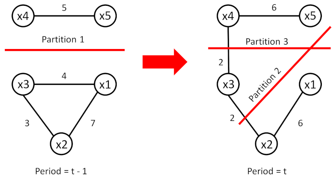
We explain the steps of the evolutionary spectral clustering algorithm by considering the following example. Figure 6 shows two graphs at time periods and t. In this example, we choose a number of classes equal to two for the two periods.
The similarity matrices of the two graphs are defined as follows:
It is clear that the graph at time period t-1 should be clustered by partition 1 when we apply the evolutionary spectral clustering algorithm. In order to partition the graph at time period t, we run the evolutionary spectral clustering algorithm by applying the framework. We obtain the following Laplacian matrix:
Next, we solve the the eigen problem. We obtain the eigenvector matrix as follows:
Since the values of U are in the interval , then we choose equal to U. Next, we compute as the ith row of . Finally, we apply the K-means algorithm to the data points and we obtain the two clusters of partition 3: and . It is shown that both partition 2 and partition 3 are good for time period t; however, partition 3 should be preferred because it is more consistent with partition 1 at time period .
2.5. Efficient Evolutionary Spectral Clustering Algorithm
A major issue of the evolutionary spectral clustering algorithm is its computational and memory cost. If we denote by N the number of the data snakes at a given time, solving the eigenvalue problem has a complexity and the evolutionary Laplacian does not fit into the main memory when N is large. To solve this problem, we define the following eigenvalue problem involving the smoothed Laplacian as follows [27]:
where
This similarity matrix for PCQ is defined as:
Notice that, in contrast to evolutionary spectral clustering, we consider all the previous time steps before the actual time point using an iterative process because of the low computation of the efficient evolutionary spectral clustering algorithm. However, the computation of the similarity matrix for PCM is not adopted for the efficient evolutionary spectral clustering algorithm. Thus, in the objective to make a comparative study with the PCM framework, we propose a similarity matrix for PCM defined as follows:
The second term of the equation is multiplied by in order to reduce the term to the identity matrix when the smoothed Laplacian is computed. To achieve the reduction of the eigenvalue problem, the similarity matrix is replaced with its incomplete Cholesky decomposition (ICD) [28].
An ICD of a matrix allows us to compute a low-rank approximation of accuracy of matrix , where with , such that . The value of m is computed by the incomplete Cholesky decomposition algorithm [28]. The ICD selects the rows and columns of , which are called pivots considering that the ranks of approximation are close to the rank of the original matrix. The first step in solving the problem with efficient evolutionary spectral clustering is to reduce the eigenvalue problem of both PCQ and PCM. Thus, we obtain . After that, we replace with its factorization and substitute R with its singular value decomposition. As a result, we will obtain the following equation:
where and such that and ,, . We have to solve an eigenvalue problem of size , involving the matrix that is smaller than the size of the original problem.
In addition, the eigenvectors problem can be estimated as , where the related eigenvalues are . At last, the cluster assignment for the ith data points are obtained from the pivoted LQ factorization of matrix :
such that is a permutation matrix as defined in [27], is a lower triangular matrix, and is the unitary matrix.
The classic ICD algorithm is based on the supposition that the Laplacian matrix has a small rank. A new stopping criterion assumes that the cluster assignments tend to converge after selecting each pivot. Therefore, for the cluster assignments at step s and atstep , the normalized mutual information (NMI) is calculated. The time step s is used for an iterative process of the algorithm. The NMI is defined by [29]:
where the mutual information between the partitions and is defined as:
The term represents the number of shared patterns between the clusters and , and is the number of clusters in partition . The entropy of the partition is defined as:
A higher NMI value means that the clustering algorithms generate identical partitions. The NMI value is bounded in (0,1), equaling 1 when the two partitions are identical and 0 when they are independent. Consequently, the ICD algorithm terminates when , where is a user-defined threshold value.
To make this procedure faster, we need to check the convergence of the cluster assignments only when the approximation of the similarity matrix is good enough. Thus, we stop the computation when the quality of the approximation of the similarity matrix is greater than a predefined threshold as follows:
where
Finally, to prevent the termination of the ICD algorithm too early with the poor and insufficient performance of clusters, we choose , which is a suitable choice through experiences. As a result, this criterion decreases the number of selected pivots and improves the computational complexity. This methodology outperforms the evolutionary spectral clustering and the normalized spectral clustering algorithm that is denoted by IND, which independently applies the spectral clustering algorithm on the speed of road segments in only the time step t and ignores all the historic data before t.
It is shown that the computational complexity of the efficient evolutionary spectral clustering algorithm is [27]. On the other hand, the methods of the evolutionary spectral clustering have a complexity of as a result of the fully eigen decomposition of the similarity matrices that are included at each time t. Consequently, this method is an effective tool for dealing with large-scale clustering problems with a time complexity of . The efficient evolutionary spectral clustering algorithm for the transportation network is given by Algorithm 3.
| Algorithm 3 Efficient Evolutionary Spectral Clustering Algorithm for Transportation Networks |
|
3. Automatically Choosing the Number of Clusters
The spectral clustering method requires knowing the number of clusters in the graph. However, in any transport network, it is difficult to know this number a priori. In order to determine the appropriate number of clusters, we introduce a novel version of the density peaks algorithm, the modularity method and the eigengap heuristic, and we compare these methods in our experiments in order to choose the appropriate method.
3.1. Density Peaks Algorithm
The density peaks algorithm, which can detect non-convex clusters, is based on two assumptions. The first one is that the cluster centers are surrounded by neighbors with lower local density. The second assumption is the clusters’ centers are at a relatively large distance from any snake with a higher local density. The density peaks algorithm uses three important variables: The local density for each snake in the whole data set, the minimum distance among snake and other snakes that have higher density [30] and the parameter , which is the product of and for each snake . Then, we choose the snakes with the largest values as centers.
We compute the local density and the minimum distance from snakes with higher density to represent the two quantities of any snake . For each snake in the whole data set of snakes , the local density is defined as follows:
where is a cutoff distance, is a kernel function, and is the distance among snakes and . For each snake , these quantities are dependent on the distance among two snakes and . In this paper, we adopted the following distance between two snakes based on the sparse snake similarity matrix as follows:
The parameter controls the marginal impact of the authentication in the case of additional similarities taking place among snakes. We choose, in our case , to obtain the densely distributed snakes in space. In fact, is the number of snakes that are too similar to a snake . On the other hand, calculating the local density using the Gaussian function can avoid having the same density values for the snakes. The results are greatly influenced by the cutoff distance . The local density is computed as follows:
The is the minimum distance from snake to the higher-density snakes and is defined as follows:
If there is one snake with the largest density, it makes a compromise with , defined as the maximal distance from itself to other snakes, which enables it to have the largest value again.
In order to select the centers, we calculate, for each snake, the parameter with the largest values. We select the K snakes that have the largest values of , such that K is the number of classes. To see whether a distance is relatively large, we should make a comparison of it with another one, so that we can model a comparison with a new quantity for and the distance between a snake and its nearest neighbor with a lower density, denoted by [30]:
The parameter shows the distance from the snake to the area with lower density. It shows how far away the snake i is from the area with lower density, which is a suitable quantity for to compare with. Consider the quantity defined as the difference between and :
The comparative magnitude of must be revealed to find the potential cluster centers. Moreover, the distance between a snake and another one with a higher density is greater than to a snake with a lower density if the . It is known that the area of low density is closer than the area of high density to a snake surrounded with a lower density. On the other hand, the snakes that have the higher density are relatively distant. Consequently, the quantity denotes the relative magnitude of . We substitute by in the decision graph and set . Thus, the center points with high values will pop-out in the decision graph.
The mutual K-nearest-neighbor graph is used in order to compute the density measure for all snakes [31]. The mutual K-nearest-neighbor graph (mKNN graph) is defined as an un-directed graph where there is an edge that connects both snakes and only if one of them belongs to the K-nearest neighbors of the other. Regarding the original definition of the density measure, the new density measure is influenced through both the cutoff distance and each distance between two points and . The new density measure is defined as follows:
where is the set of connected snakes in the mKNN graph for each snake . The mKNN graph provides a clear direction if a snake must be revealed in the calculation of . The minimum distance from snake to the higher-density snake is still the same as the original definition that is defined in Equation (35). In order to find the number of class centers, we can plot, for each snake, the to detect the centers and select the cluster centers using the following formula:
such that the threshold is a parameter selected by the user. However, this method cannot determine the parameter for different data sets. In this paper, this problem is solved with a statistic-based approach to identify the cluster centers from the decision graph automatically. This approach is based on the minimum distance to be much larger than among the nearest neighbors’ distances only when the snake has the maximum density.
This provides an important feature that specifies the cluster center using an outlier detection that includes the probability density function in the decision graph at a particular density [32]. The outliers are specified by the following threshold :
The two parameters and are defined as follows:
where a and b are the two-dimensional kernel widths. They are defined as follows:
where and are the standard deviations of and for all the snakes. The two parameters and are user-defined parameters used to identify the cluster center and compute the value. We specify a snake as a class center when the minimum distance . However, the performance of the density peaks algorithm depends on the-off distance . To avoid this limitation, the value of is automatically extracted from the set of snakes by minimizing a potential entropy defined as follows [33]:
where is a normalization factor. The density peaks algorithm for the transportation network is given by Algorithm 4.
| Algorithm 4 Density Peaks for Detecting the Number of Partitions in a Transportation Network |
|
3.2. Eigengap Heuristic
This method consists of finding the number of Laplacian eigenvalues such that the first k eigenvalues are small, and is relatively high [25]. This means that one should sort the eigenvalues in descending order, because it is a trace maximization problem, and find a gap in these values. We define the gap as the maximum difference between two successive eigenvalues as:
where is the maximum number of clusters. The value of the eigengap for subsequent eigenvalues will indicate where the number of clusters should be selected. The number of clusters K is given by:
However, if the distribution of the eigenvalues is uniform, the determined K is not always relevant.
3.3. Modularity
Modularity is one measure of the graph structure. It is designed to measure the strength of the division of a graph into clusters. The networks with high modularity have dense connections between nodes within the same cluster but sparse connections between nodes in different clusters. We calculate the modularity versus the number of clusters or groups. The optimum number of clusters is the one that maximizes modularity [34,35].
Given a graph and a partition of the nodes V into K clusters , the modularity is expressed as follows [34]:
where is the size of cluster . The term measures the sum of weights within the cluster and measures the sum of weights over all edges attached to nodes in cluster . The term calculates the total sum of all edge weights in the graph G.
We compute the modularity for each value of K, such as . In order to select the number of clusters, we choose the number K that maximizes the modularity function. A high value of the modularity function means that the edges within the clusters outnumber those in a similar randomly generated graph. Modularity is often used in optimization methods for detecting homogeneous cluster structures in networks.
4. Experimental Results
In this section, we analyze experimental data processed in [17] to show the performance and effectiveness of the proposed method on a network of links. Next, we automatically detect the number of clusters, and we present a comparative study between the static spectral clustering and the efficient evolutionary spectral clustering frameworks.
4.1. Transportation Network
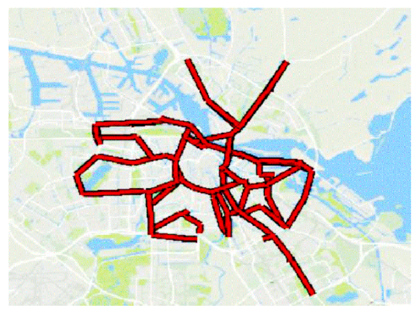
The real data were collected from Amsterdam city, and the original mapping of the inner-city network included 7512 roads [17]. The Amsterdam network of roads has been reduced to 208 roads as illustrated in Figure 7. The present study concentrates only on one day of data, which is a weekday, and the road speeds are estimated from the individual travel times. Moreover, the average speed information is available every time period of 10 min from 7 a.m. to 3 p.m. for the 208 roads. The day has a total of 48 periods, and the maximum speed of the road is 40 m/s.
4.2. Snake Length and Weight Coefficient Optimization
One of the main drawbacks of snake similarity is its heavy computational cost. A sensitivity analysis is conducted to investigate the performance of snakes for different lengths [17]. The snake length has to be set at a minimal threshold to keep the connectivity. Thus, a snake that is too short cannot discover the entire topology of the network in both space and time. A short snake length may also provide cluster results in which a cluster contains links that are not all connected with each other. The connected clusters’ dissimilarity (CCD) is used to evaluate the performance of the algorithm for different snake lengths and weight coefficient values. The CCD metric focuses on the inter-cluster dissimilarity between a given cluster and its neighboring cluster. It is defined by [17]:
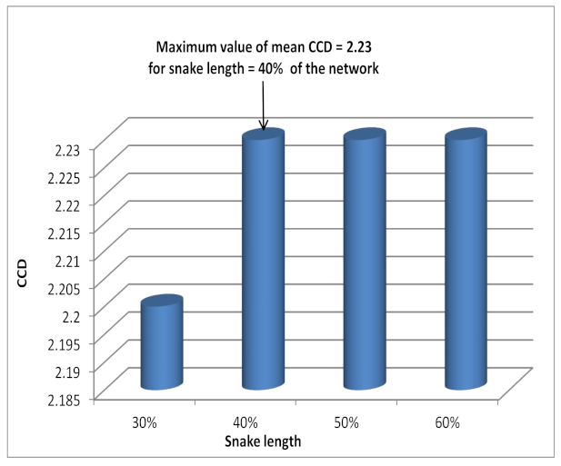
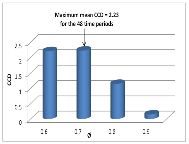
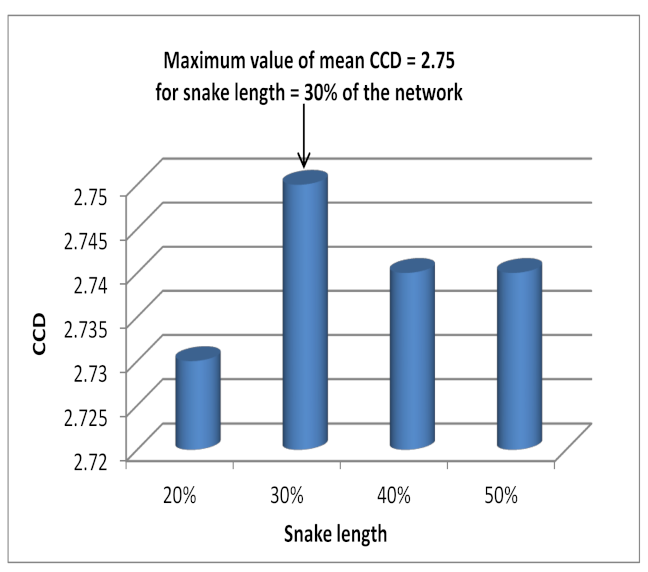
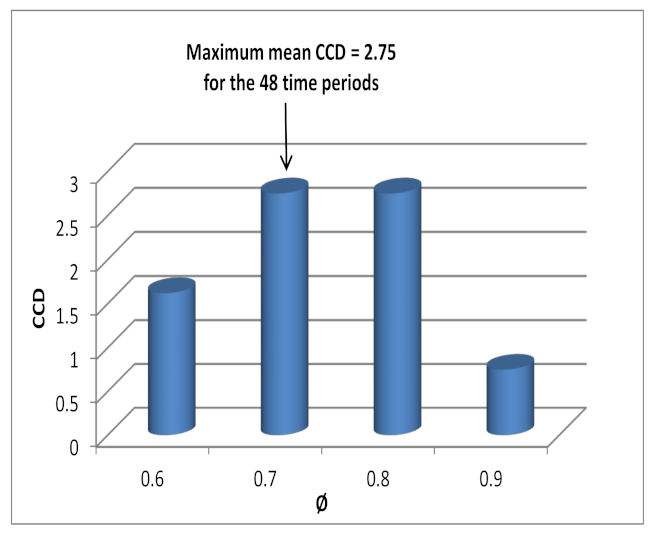
where is the mean speed of the cluster i, if i and k are the indices of connected clusters and otherwise. This evaluation metric is to be maximized. The mean values of CCD for the 48 periods are computed using different snake lengths based on the percentage of the spatio-temporal size of the network roads (Figure 8). It is clear that the algorithm produces similar results for snake lengths bigger than of the spatio-temporal size of the network of roads. Therefore, the length of the snake is set to , and the weight coefficient is selected to be equal to in order to obtain the maximum mean values of CCD (Figure 9).
4.3. Comparative Study for the Automatic Selection of the Number of Clusters
Choosing the optimal number of clusters is usually a tricky problem for all clustering algorithms. In our previous work, we considered only two clusters in order to differentiate between congested and fluid zones [19]. However, selecting a fixed number of clusters for all periods causes a strong restriction. In this section, we present a comparative study between the density peak, the eigengap [25] and the modularity [12] methods to automatically detect the number of clusters.
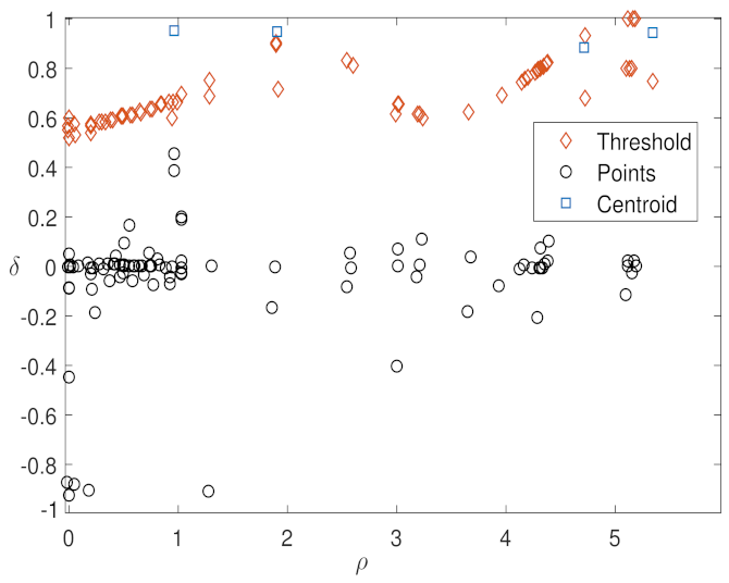
In the case of the density peak, we choose the cut-off distance that minimizes the potential entropy of data for all time periods, we compute the local density and the parameter , and we identify the cluster centers by calculating the probability density function and choosing the appropriate threshold by selecting the values of and based on [32] (Figure 10).
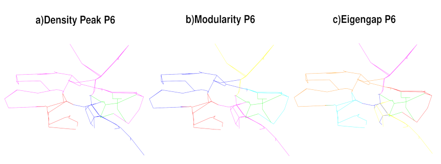
The clustering results are analyzed in the case of spectral clustering using the density peaks, the modularity and the eigengap for the automatic selection of the number of clusters. We consider the time period in order to test the three methods on a different number of clusters. We plot the results of the clustering of Amsterdam road networks (Figure 11), and we compute the average speed and the standard deviation in each cluster for time period (Table 1). It is shown that the obtained clusters have small standard deviation values, which proves a promising performance in separating homogeneous connected clusters. Moreover, the density peak algorithm is better in the partitioning of the transportation network into homogeneous partitions with separated average speed.
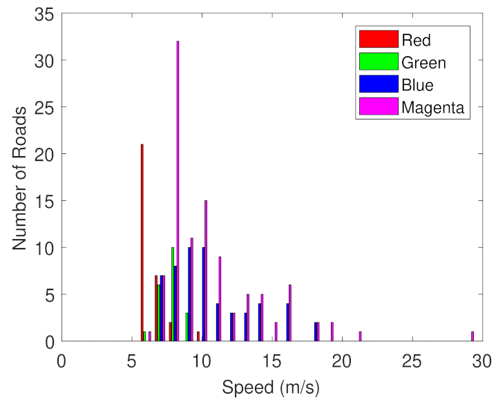
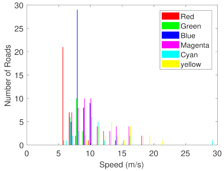
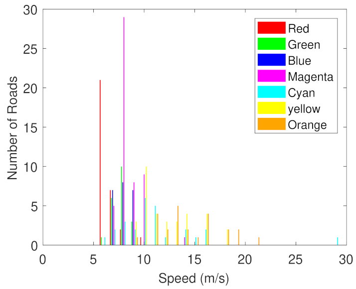
The results of the clustering method with the histogram of speeds for the density peak, the modularity and the eigengap methods are shown in Figure 12, Figure 13 and Figure 14. It can be inferred from the clustering results that the density peak algorithm can separate the pockets of congestion better than the modularity and the eigengap methods. It is clear that, in the case of density peaks, the network has two main pockets of congestion, the cluster with small average speed represented by the red color and the cluster with a higher average speed represented by the Magenta color. The other two clusters detect part of the highway with medium average speed.
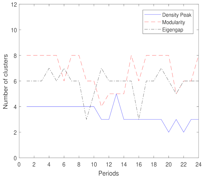
Figure 15 shows the number of clusters obtained by applying the density peak, the modularity and the eigengap methods for each time period. We find that the number of clusters obtained by the density peaks algorithm is smaller than that of the modularity and the eigengap methods. Therefore, considering a smaller number of clusters makes the interpretation easier and helps to design more efficient control strategies [7].
Next, we run the IND, PCQ and PCM using the efficient spectral clustering algorithm with the density peak, the modularity and the eigengap for selecting the number of clusters. We report all costs in Table 2, where the best results are in bold face.
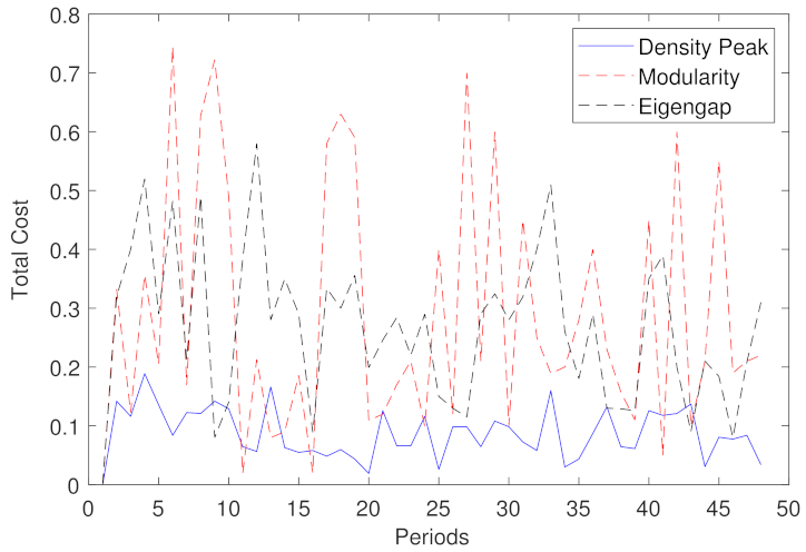
It is clear that the density peak algorithm gives the best results in minimizing the cost measures. For each time period, Figure 16 shows the variation of the total cost for the PCQ framework in the case of the density peaks, the modularity and the eigengap methods.
We did not plot the results for PCM, which were similar to those of PCQ. It is shown that the density peak, the eigengap and the modularity methods partition the transportation network equally well. However, according to temporal smoothness, the density peak method should be preferred because it is more consistent with the recent history and gives the minimum total cost for PCQ and PCM.
4.4. Comparative Study between the Spectral Clustering Algorithms
In our experiments, we compared the efficient evolutionary spectral clustering frameworks with the normalized efficient spectral clustering algorithm, which we named IND [36]. The IND method applies partitioning on the snakes at current time period t and ignores all historic data before the current time period. The number of clusters for the two efficient evolutionary spectral clustering frameworks (PCQ and PCM) and the IND method is automatically detected using the density peak method.
First, we compute the average link speeds and the standard deviation for time period with the objective of validating the effectiveness of the efficient evolutionary spectral clustering frameworks in separating homogeneous connected clusters. The results of the evaluation metrics are presented in detail in Table 3.
By comparing the mean values of link speeds and the standard deviation in different clusters, it is clear that the mean link speeds between the partitions are dissimilar for PCQ and PCM because they give a good separation between partitions. Moreover, the small value of the standard deviation for each cluster defines good intra-cluster homogeneity.
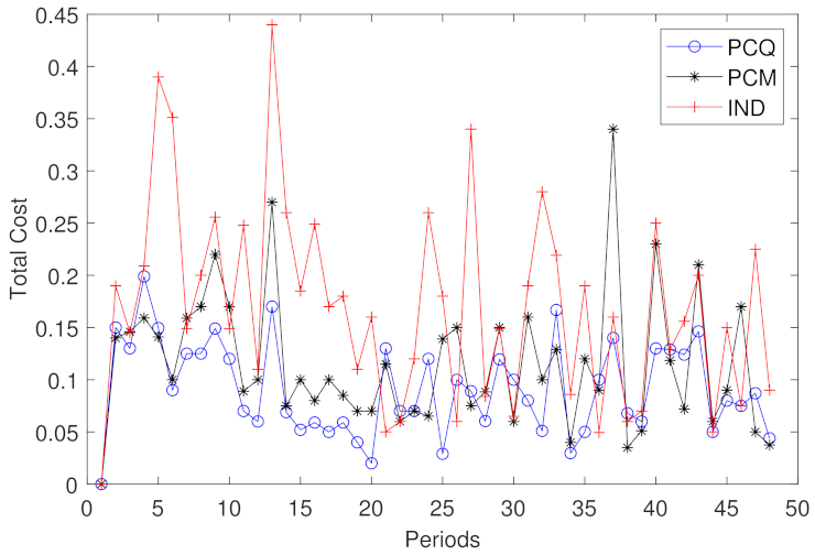
Next, we consider all time periods from to , and we evaluate the total cost values for all three methods. For all costs, a lower value means better results. Figure 17 shows the results of the total cost for the IND method and for both PCQ and PCM frameworks. As can be seen, the PCQ and PCM are better at minimizing the total cost measure over the IND method.
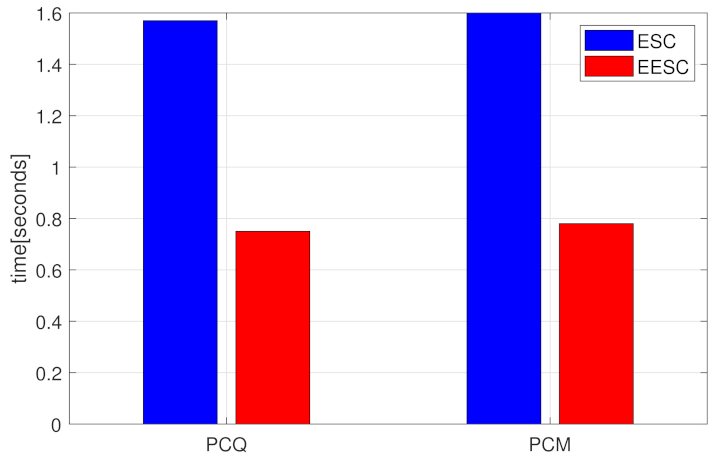
We compare the average runtime in seconds for one period using the PCQ and the PCM frameworks. The time is computed for the 48 periods, and we take the average time using MATLAB on a PC with two Intel CPUs at 2.33 GHZ and eight gigabytes of RAM. It is clear that the two frameworks of the new methodology induce a better performance in computational time than does the evolutionary spectral algorithm (Figure 18).
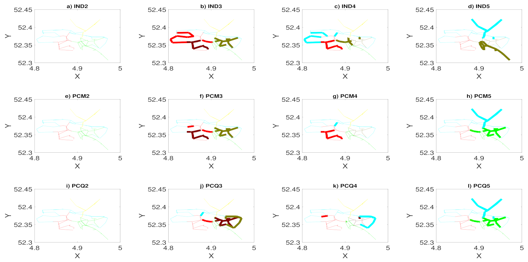
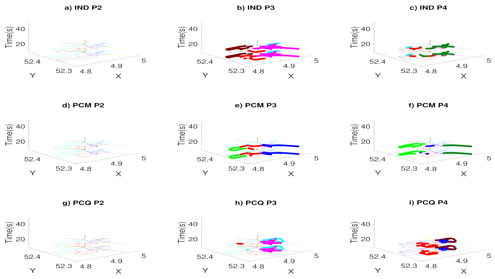
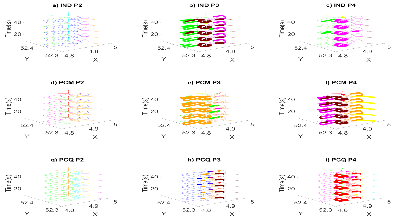
In order to validate the performance and the smoothness of the evolutionary spectral clustering frameworks in finding clusters that fit the current data while simultaneously not deviating from previous history, in this experiment, we plot the partitioning results of the Amsterdam network for the PCQ, PCM and IND methods. In order to match the clusters between consecutive time-steps, we used the Kuhn–Munkres Hungarian algorithm, which performs one-to-one cluster matching between consecutive partitioning based on the number of common links between clusters [37,38].
This algorithm, which is the most popular polynomial time algorithm for solving classical assignment problems, allows us to follow the evolution of the clusters over time. Figure 19 illustrates the partitioning results with the number of clusters detected automatically by the density peak method. The analyzed time periods are from to , which corresponds to day hours from 7:10–7:40 a.m, one of the peak times of a weekday.
The bold color represents the links specifying the deviation from one cluster to another. For time periods to , we find that, for the IND method, the number of links in a cluster changes rapidly. However, the PCM and PCQ frameworks are more stable when compared to the historic data. It is shown that the PCQ and PCM frameworks assure the best performance and give more stable and consistent cluster results compared with the IND method.
Next, we set the time period to 20 min. We consider the neighborhood of a link in both space and time, and we make a duplicate of the links at time period . In fact, we consider the graph with link speeds at time period t and the graph with link speeds at time period .
The length of the snake is set to , and we choose in order to assure the maximum mean values of CCD (Figure 20 and Figure 21). Figure 22 shows the number of clusters obtained by applying the density peak method for time periods to .
Figure 23 shows the partitioning results for time periods to . It is clear that the PCQ framework gives more stable and consistent cluster results than the PCM and IND methods.
Finally, we set the time period to one hour. We consider the neighborhood of a link in both space and time, and we make a duplicate of the links at time period and . The length of the snake is set to of the network size in order to minimize the computation complexity, and we choose .
Figure 24 shows the partitioning results for time periods to . It is clear that, for all experiments, the PCQ framework gives more stable and consistent cluster results compared with the PCM and the IND methods. These experiments, based on real data collected from Amsterdam city, demonstrate that, compared to traditional clustering methods, our efficient evolutionary spectral clustering algorithm has the advantage of finding directional congestion within stable and consistent clusters, which allows us to design real-time traffic control schemes—specifically, hierarchical perimeter control approaches to alleviate or postpone congestion.
5. Conclusions
The goal of our study was to partition a transportation network by incorporating temporal smoothness in evolutionary spectral clustering. We presented two frameworks for partitioning the network. In the first framework, the temporal cost is expressed as how well the current partition clusters the historic variation of link speeds. The second framework is different from the first regarding how the temporal smoothness is measured. In this framework, the temporal cost is expressed as the difference between the current partition and the historic one. In both frameworks, a cost function is defined in order to regularize the temporal smoothness.
In order to determine the appropriate number of clusters, we used the density peak algorithm, which we proved to be efficient when compared with the modularity and the maximum eigengap methods. Experimental studies on the Amsterdam city network demonstrated that the two efficient evolutionary spectral clustering frameworks provided results that are stable and consistent in an environment where traffic can change over time.
In future work, we will address the following constraints and limitations. We will consider the case where some sensors do not provide valid measurements for specific time intervals. We will extend our efficient evolutionary spectral algorithm to be applied in the case of missing speed data. We will also consider the case of the insertion and removal of links in the network.
In a transportation network, a road can either be closed or opened. In this case, the size of the similarity matrix can change between time periods. Moreover, we will work on another promising application for the partitions computed by efficient evolutionary spectral clustering, which is to predict future travel times using deep-learning algorithms.
6. Code and Data Availability Policies
Code are however available from the authors upon reasonable request and with permission of the LISIC Laboratory.The data related to this study are accessible using the following link: https://doi.org/10.6084/m9.figshare.5198566 (accessed on 19 January 2022).
Author Contributions
Conceptualization, J.C. and I.C.; methodology, P.A.A. and J.C.; software, P.A.A. and J.C.; validation, I.C. and C.L.; formal analysis, J.C. and I.C.; investigation, J.C. and C.L.; data curation, C.L.; writing—original draft preparation, P.A.A.; writing—review and editing, J.C. and I.C.; project administration, J.C.; funding acquisition, P.A.A. and C.L. All authors have read and agreed to the published version of the manuscript.
Funding
This project has received funding from the “Paprika IA Développement” company and the project National Natural Science Foundation of China (71971014) named “Study on the Dynamic Traffic Assignment Problem with Graphical Solution Method”. This project has also received funding from the ERIC laboratory at the University of Lyon, Lyon 2, ERIC UR 3083, 5 avenue Pierre Mendès France, F69676 Bron Cedex, France. This work was funded in part by the Université du Littoral Côte d’Opale in France and the Agence Universitaire de la Francophonie with the National Council for Scientific Research in Lebanon through a doctoral fellowship grant under ARCUS E2D2 project.
Institutional Review Board Statement
Not applicable.
Informed Consent Statement
Not applicable.
Data Availability Statement
Not applicable.
Conflicts of Interest
Each author certifies that this material or similar material has not been and will not be submitted to or published in any other publication.
Glossary
The following abbreviations are used in this manuscript:
| N | Number of snakes |
| L | Size of the snake |
| K | Number of clusters |
| T | Number of periods |
| Maximum number of clusters | |
| Network of links | |
| I | Set of intersections in the network of links |
| R | Set of links in the network of links |
| V | Set of nodes in the graph of links |
| E | Set of links in the graph of links |
| G | Graph of snakes |
| Set of vertices in the graph of snakes | |
| Similarity between snakes | |
| Identifier for snake i | |
| Link identifier | |
| Link speed | |
| Variance of the snake at each step l | |
| Mean speed of the snake at each step l | |
| Element of the similarity matrix | |
| Weight coefficient | |
| C | Set of clustering results |
| Normalized cut variable | |
| Laplacian matrix | |
| Z | Indicator matrix for a partition |
| D | Degree matrix |
| X | Matrix of eigenvectors |
| Snapshot cost | |
| Temporal cost | |
| Parameter that reflects the user’s emphasis on the snapshot cost | |
| Parameter that reflects the user’s emphasis on the temporal cost () | |
| Laplacian matrix for preserving cluster quality | |
| Laplacian matrix for preserving cluster membership | |
| The ith eigenvalue | |
| U | Matrix containing the eigenvectors |
| Laplacian for efficient evolutionary spectral clustering | |
| P | Low-rank matrix approximation of the similarity matrix |
| Y | Permutation matrix used to compute the cluster assignment |
| Cluster assignment of the ith data point | |
| Normalized mutual information | |
| Mutual information | |
| Entropy of partition | |
| Threshold used to terminate the efficient evolutionary spectral clustering | |
| Threshold used to terminate the incomplete Cholesky decomposition | |
| Local density | |
| Cutoff distance | |
| Minimum distance from snake to the higher-density snakes | |
| Parameter used to find the potential cluster centers | |
| Distance from the snake to the area with lower density | |
| Parameter used to select the cluster centers | |
| User-defined parameter used to identify the cluster center | |
| User-defined parameter used to identify the cluster center | |
| H | Entropy used to find |
| Threshold used to find the number of clusters | |
| Mean value used to select | |
| Standard deviation used to find | |
| Maximum difference between two successive eigenvalues | |
| M | Modularity variable |
| Connected cluster dissimilarity |
References
- Pojani, D.; Stead, D. Sustainable Urban Transport in the Developing World: Beyond Megacities. Sustainability 2015, 7, 7784–7805. [Google Scholar] [CrossRef] [Green Version]
- Farhi, N.; Phu, C.N.V.; Amir, M.; Haj-Salem, H.; Lebacque, J.P. A Semi-decentralized Control Strategy for Urban Traffic. Transp. Res. Procedia 2015, 10, 41–50. [Google Scholar] [CrossRef] [Green Version]
- Ognjenović, S.; Zafirovski, Z.; Vatin, N. Planning of the Traffic System in Urban Environments. Procedia Eng. 2015, 117, 574–579. [Google Scholar] [CrossRef]
- Leontiadis, I.; Marfia, G.; Mack, D.; Pau, G.; Mascolo, C.; Gerla, M. On the Effectiveness of an Opportunistic Traffic Management System for Vehicular Networks. IEEE Trans. Intell. Transp. Syst. 2011, 12, 1537–1548. [Google Scholar] [CrossRef] [Green Version]
- Yuan, J.; Zheng, Y.; Xie, X.; Sun, G. Driving with knowledge from the physical world. In Proceedings of the 17th ACM SIGKDD International Conference on Knowledge Discovery and Data Mining, San Diego, CA, USA, 21–24 August 2011. [Google Scholar]
- Saeedmanesh, M.; Geroliminis, N. Dynamic clustering and propagation of congestion in heterogeneously congested urban traffic networks. Transp. Res. Part B 2017, 105, 193–211. [Google Scholar] [CrossRef]
- Ji, Y.; Geroliminis, N. On the spatial partitioning of urban transportation networks. Transp. Res. Part B 2012, 46, 1639–1656. [Google Scholar] [CrossRef] [Green Version]
- Saeedmanesh, M.; Geroliminis, N. Clustering of heterogeneous networks with directional flows based on “Snake” similarities. Transp. Res. Part B Methodol. 2016, 91, 250–269. [Google Scholar] [CrossRef] [Green Version]
- Nanni, M.; Pedreschi, D. Time-focused clustering of trajectories of moving objects. J. Intell. Inf. Syst. 2006, 27, 267–289. [Google Scholar] [CrossRef]
- Jeung, H.; Shen, H.T.; Zhou, X. Convoy queries in spatio-temporal databases. In Proceedings of the 2008 IEEE 24th International Conference on Data Engineering, Cancun, Mexico, 7–12 April 2008; pp. 1457–1459. [Google Scholar]
- El Mahrsi, M.K.; Rossi, F. Modularity-based clustering for network-constrained trajectories. arXiv 2012, arXiv:1205.2172. [Google Scholar]
- El Mahrsi, M.K.; Rossi, F. Graph-Based Approaches to Clustering Network-Constrained Trajectory Data. 2012. Available online: http://xxx.lanl.gov/abs/1210.0762 (accessed on 19 January 2022).
- Kouvelas, A.; Saeedmanesh, M.; Geroliminis, N. Enhancing model-based feedback perimeter control with data-driven online adaptive optimization. Transp. Res. Part B 2017, 96, 26–45. [Google Scholar] [CrossRef] [Green Version]
- Khalid, A.; Umer, T.; Azfal, M.; Anjum, S.; Sohail, A.; Asif, H.M. Autonomuous data driven surveillance and rectification system using in vehicle sensors for intelligence transportation system (ITS). Comput. Netw. 2018, 139, 109–118. [Google Scholar] [CrossRef]
- Chen, C.; Xiang, H.; Qiu, T.; Wang, C.; Zhou, Y.; Chang, V. A rear end collision prediction scheme based on deep learning in the internet of vehicles. Parallel Distrib. Comput. 2018, 117, 192–204. [Google Scholar] [CrossRef]
- Tuffery, S. Data Mining and Statistics for Decision Making, 2nd ed.; John Wiley and Sons, Ltd.: Chichester, UK, 2011; pp. 43–91. [Google Scholar]
- Lopez, C.; Krishnakumari, P.; Leclercq, L.; Chiabaut, N.; Lint, H.V. Spatio-temporal partitioning of transportation network using travel time data. Transp. Res. Rec. J. Trasp. Res. 2017, 2623, 98–107. [Google Scholar] [CrossRef] [Green Version]
- Chi, Y.; Song, X.; Zhou, D.; Hino, K.; Tseng, B.L. Evolutionary Spectral Clustering by Incorporating Temporal Smoothness. In Proceedings of the 13th ACM SIGKDD International Conference on Knowledge Discovery and Data Mining, San Jose, CA, USA, 12–15 August 2007. [Google Scholar]
- Al Alam, P.; Hamad, D.; Constantin, J.; Constantin, I.; Zaatar, Y. Dynamic Partitioning of Transportation Network Using Evolutionary Spectral Clustering. In Proceedings of the Smart Applications and Data Analysis, Third International Conference, Marrakesh, Morocco, 25–26 June 2020; pp. 178–186. [Google Scholar]
- Dinh, D.T.; Fujinami, T.; Huynh, V.N. Estimating the Optimal Number of Clusters in Categorical Data Clustering by Silhouette Coefficient. In International Symposium on Knowledge and Systems Sciences; Springer: Singapore, 2019; pp. 1–17. [Google Scholar]
- Astolfi, D.; Pandit, R. Multivariate Wind Turbine Power Curve Model Based on Data Clustering and Polynomial LASSO Regression. Appl. Sci. 2022, 12, 72. [Google Scholar] [CrossRef]
- Tibshirani, R.; Walther, G.; Hastie, T. Estimating the number of clusters in a data set via the gap statistic. J. R. Stat. B 2001, 63, 411–423. [Google Scholar] [CrossRef]
- Salvador, S.; Chan, P. Determining the number of clusters/segments in hierarchical clustering/segmentation algorithms. In Proceedings of the 16th IEEE International Conference on Tools with Artificial Intelligence, Boca Raton, FL, USA, 15–17 November 2004; pp. 576–584. [Google Scholar] [CrossRef] [Green Version]
- Lopez, C. Modélisation Dynamique du Trafic et Transport de Marchandises en Ville: Vers une Approche Combinée. Ph.D. Thesis, Université de Lyon, Lyon, France, 2017. [Google Scholar]
- Von Luxburg, U. A tutorial on spectral clustering. Stat. Comput. 2007, 17, 395–416. [Google Scholar] [CrossRef]
- Shi, J.; Malik, J. Normalized cuts and image segmentation. IEEE Trans. Pattern Anal. Mach. Intell. 2000, 22, 888–905. [Google Scholar]
- Langone, R.; Van Barel, M.; Suykens, J.A. Efficient evolutionary spectral clustering. Pattern Recognit. Lett. 2016, 84, 78–84. [Google Scholar] [CrossRef]
- Frederix, K.; Barel, M.V. Sparse spectral clustering method based on the incomplete Cholesky decomposition. J. Comput. Appl. Math. 2013, 237, 145–161. [Google Scholar] [CrossRef]
- Meila, M. Comparing clusterings—An information based distance. J. Multivar. Anal. 2007, 98, 873–895. [Google Scholar] [CrossRef] [Green Version]
- Li, Z.; Tang, Y. Comparative density peaks clustering. Expert Syst. Appl. 2018, 95, 236–247. [Google Scholar] [CrossRef]
- Zhang, H.; Kiranyaz, S.; Gabbouj, M. Data Clustering Based on Community Structure in Mutual k-Nearest Neighbor Graph. In Proceedings of the 41st International Conference on Telecommunications and Signal Processing (TSP), Athens, Greece, 4–6 July 2018; pp. 262–268. [Google Scholar]
- Yan, H.; Lu, Y.; Ma, H. Density-based Clustering using Automatic Density Peak Detection. In Proceedings of the International Conference on Pattern Recognition Applications and Methods, Madeira, Portugal, 16–18 January 2018. [Google Scholar]
- Wang, S.; Wang, D.; Li, C.; Li, Y. Comment on “Clustering by Fast Search and Find of Density Peaks”. 2015. Available online: http://xxx.lanl.gov/abs/1501.04267 (accessed on 19 January 2022).
- Yu, L.; Ding, C. Network community discovery: Solving modularity clustering via normalized cut. In Proceedings of the Eighth Workshop on Mining and Learning with Graphs, Washington, DC, USA, 24–25 July 2010. [Google Scholar]
- Scott, W.; Padhraic, S. A Spectral Clustering Approach To Finding Communities in Graphs. In Proceedings of the 2005 SIAM International Conference on Data Mining, Newport Beach, CA, USA, 21–23 April 2005. [Google Scholar]
- Ng, A.Y.; Jordan, M.I.; Weiss, Y. On spectral clustering: Analysis and an algorithm. In Proceedings of the Advances in Neural Information Processing Systems, Vancouver, BC, Canada, 3–8 December 2001. [Google Scholar]
- Xu, K.; Kliger, M.; Hero, A. Adaptive evolutionary clustering. Data Min. Knowl. Discov. 2014, 28, 304–336. [Google Scholar] [CrossRef] [Green Version]
- Hong, C.; Jingjing, Z.; Chunfeng, C.; Qinyu, C. Solving large-scale assignment problems by Kuhn-Munkres algorithm. In Proceedings of the 2nd International Conference on Advances in Mechanical Engineering and Industrial Informatics, Hangzhou, China, 9–10 April 2016. [Google Scholar]
Figure 1.
A data flow chart describing our methodological steps.

Figure 2.
The two graph models are explained using two different examples. (a) The primal graph model, which consists of representing the intersections by nodes and the roads by edges. (b) The dual graph model, which consists of considering the roads as the graph nodes and the crossing point between them as edges.

Figure 3.
Example of a snake initialized by a link in red. The green links represent the neighborhood, according to a 2D approach (a) and a 3D approach (b) [24].
Figure 3.
Example of a snake initialized by a link in red. The green links represent the neighborhood, according to a 2D approach (a) and a 3D approach (b) [24].

Figure 4.
Variance of two snakes of the graph of links.

Figure 5.
Snake computed on the network of the sixth district of Paris. The number of links in the snake is equal to 64.
Figure 5.
Snake computed on the network of the sixth district of Paris. The number of links in the snake is equal to 64.

Figure 6.
Two graphs at time periods and t.

Figure 7.
Amsterdam reduced network with 208 roads [24].
Figure 7.
Amsterdam reduced network with 208 roads [24].

Figure 8.
The mean values of connected clusters’ dissimilarity versus snake length computed as a percentage of the size of the network of roads.
Figure 8.
The mean values of connected clusters’ dissimilarity versus snake length computed as a percentage of the size of the network of roads.

Figure 9.
The mean values of connected clusters’ dissimilarity versus the weight coefficient .

Figure 10.
Decision graph for the time period using the density peak algorithm and the probability density function.
Figure 10.
Decision graph for the time period using the density peak algorithm and the probability density function.

Figure 11.
Clustering results for the time period in the case of the density peak (a), modularity (b) and eigengap (c).
Figure 11.
Clustering results for the time period in the case of the density peak (a), modularity (b) and eigengap (c).

Figure 12.
Histogram of link speeds for the time period = 6 in the case of the density peak.

Figure 13.
Histogram of link speeds for the time period = 6 in the case of the modularity.

Figure 14.
Histogram of link speeds for the time period = 6 in the case of the eigengap.

Figure 15.
The number of clusters obtained by applying the density peak, the modularity and the eigengap methods for each time period.
Figure 15.
The number of clusters obtained by applying the density peak, the modularity and the eigengap methods for each time period.

Figure 16.
Variation of the total cost for the PCQ framework using the density peak, the modularity and the eigengap methods. The total cost function is defined as a linear combination of the snapshot cost (SC) and the temporal cost (TC).
Figure 16.
Variation of the total cost for the PCQ framework using the density peak, the modularity and the eigengap methods. The total cost function is defined as a linear combination of the snapshot cost (SC) and the temporal cost (TC).

Figure 17.
Variation of the total cost for each time period in the case of time period = 10 min.

Figure 18.
Comparing the average runtimes of the Evolutionary Spectral Clustering (ESC) and the Efficient Evolutionary Spectral Clustering (EESC) algorithms for PCQ and PCM frameworks.
Figure 18.
Comparing the average runtimes of the Evolutionary Spectral Clustering (ESC) and the Efficient Evolutionary Spectral Clustering (EESC) algorithms for PCQ and PCM frameworks.

Figure 19.
Clustering results for time periods from to for the IND, PCM and PCQ methods in the case of time period = 10 min.
Figure 19.
Clustering results for time periods from to for the IND, PCM and PCQ methods in the case of time period = 10 min.

Figure 20.
The mean values of connected clusters’ dissimilarity versus snake length computed in the percentage of the size of the network of roads in the case of time period = 20 min.
Figure 20.
The mean values of connected clusters’ dissimilarity versus snake length computed in the percentage of the size of the network of roads in the case of time period = 20 min.

Figure 21.
The mean values of connected clusters’ dissimilarity versus the weight coefficient in the case of time period = 20 min.
Figure 21.
The mean values of connected clusters’ dissimilarity versus the weight coefficient in the case of time period = 20 min.

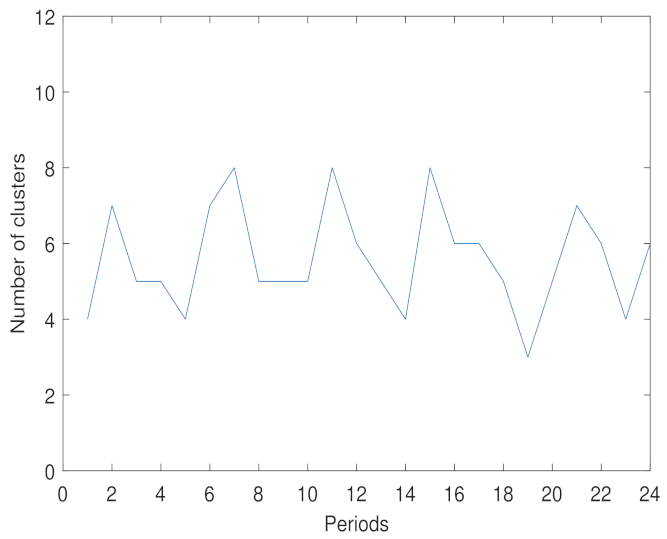
Figure 22.
The number of clusters obtained by applying the density peak method for each time period in the case of time period = 20 min.
Figure 22.
The number of clusters obtained by applying the density peak method for each time period in the case of time period = 20 min.

Figure 23.
Clustering results for time periods from to for the IND, PCM and PCQ methods in the case of time period = 20 min.
Figure 23.
Clustering results for time periods from to for the IND, PCM and PCQ methods in the case of time period = 20 min.

Figure 24.
Clustering results for time periods from to for the IND, PCM and PCQ methods in the case of a time period equal to one hour.
Figure 24.
Clustering results for time periods from to for the IND, PCM and PCQ methods in the case of a time period equal to one hour.


Table 1.
Average speed values (m/s) over standard deviation (average speed/standard deviation) for a time period with number of clusters in the case of density peaks, in the case of the modularity method and in the case of eigengap.
Table 1.
Average speed values (m/s) over standard deviation (average speed/standard deviation) for a time period with number of clusters in the case of density peaks, in the case of the modularity method and in the case of eigengap.
| Cluster | Red | Green | Blue | Magenta | Cyan | Yellow | Orange |
|---|---|---|---|---|---|---|---|
| Density Peaks | n.a. | n.a. | n.a. | ||||
| Modularity | n.a. | ||||||
| Eigengap |
Table 2.
Performance under the density peak, the modularity and the eigengap algorithms.
| IND | PCQ | PCM | ||
|---|---|---|---|---|
| Modularity | SC | 0.28 | 0.29 | 0.30 |
| TC | 0.67 | 0.34 | 0.42 | |
| Total Cost | 0.44 | 0.31 | 0.35 | |
| Eigengap | SC | 0.24 | 0.25 | 0.28 |
| TC | 0.60 | 0.30 | 0.31 | |
| Total Cost | 0.38 | 0.27 | 0.29 | |
| Density Peak | SC | 0.11 | 0.08 | 0.10 |
| TC | 0.25 | 0.10 | 0.12 | |
| Total Cost | 0.17 | 0.09 | 0.11 |
Table 3.
Average speed values (m/s) over standard deviation (average speed/standard deviation) for time period in the case of the IND, PCQ and PCM frameworks.
Table 3.
Average speed values (m/s) over standard deviation (average speed/standard deviation) for time period in the case of the IND, PCQ and PCM frameworks.
| Cluster | Red | Green | Blue | Magenta |
|---|---|---|---|---|
| IND | 6.03/0.79 | 7.17/0.74 | 9.98/2.86 | 10.03/3.63 |
| PCQ | 7.25/1.38 | 9.52/4.05 | 10.03/2.86 | 13.72/3.06 |
| PCM | 7.05/1.32 | 9.44/2.82 | 10.02/3.81 | 13.72/3.06 |
Publisher’s Note: MDPI stays neutral with regard to jurisdictional claims in published maps and institutional affiliations. |
© 2022 by the authors. Licensee MDPI, Basel, Switzerland. This article is an open access article distributed under the terms and conditions of the Creative Commons Attribution (CC BY) license (https://creativecommons.org/licenses/by/4.0/).
Share and Cite
MDPI and ACS Style
Al Alam, P.; Constantin, J.; Constantin, I.; Lopez, C. Partitioning of Transportation Networks by Efficient Evolutionary Clustering and Density Peaks. Algorithms 2022, 15, 76. https://doi.org/10.3390/a15030076
AMA Style
Al Alam P, Constantin J, Constantin I, Lopez C. Partitioning of Transportation Networks by Efficient Evolutionary Clustering and Density Peaks. Algorithms. 2022; 15(3):76. https://doi.org/10.3390/a15030076
Chicago/Turabian StyleAl Alam, Pamela, Joseph Constantin, Ibtissam Constantin, and Clelia Lopez. 2022. "Partitioning of Transportation Networks by Efficient Evolutionary Clustering and Density Peaks" Algorithms 15, no. 3: 76. https://doi.org/10.3390/a15030076
Note that from the first issue of 2016, this journal uses article numbers instead of page numbers. See further details here.