On the Use of Learnheuristics in Vehicle Routing Optimization Problems with Dynamic Inputs


1
IN3—Computer Science Department, Open University of Catalonia, 08018 Barcelona, Spain
2
Euncet Business School, 08225 Terrassa, Spain
3
Centre de Recerca Matemàtica, 08193 Bellaterra, Spain
4
Barcelona Supercomputing Center, 08034 Barcelona, Spain
*
Author to whom correspondence should be addressed.
Algorithms 2018, 11(12), 208; https://doi.org/10.3390/a11120208
Submission received: 21 November 2018
/
Revised: 10 December 2018
/
Accepted: 13 December 2018
/
Published: 15 December 2018
(This article belongs to the Special Issue Algorithms for Decision Making)
Abstract
:Freight transportation is becoming an increasingly critical activity for enterprises in a global world. Moreover, the distribution activities have a non-negligible impact on the environment, as well as on the citizens’ welfare. The classical vehicle routing problem (VRP) aims at designing routes that minimize the cost of serving customers using a given set of capacitated vehicles. Some VRP variants consider traveling times, either in the objective function (e.g., including the goal of minimizing total traveling time or designing balanced routes) or as constraints (e.g., the setting of time windows or a maximum time per route). Typically, the traveling time between two customers or between one customer and the depot is assumed to be both known in advance and static. However, in real life, there are plenty of factors (predictable or not) that may affect these traveling times, e.g., traffic jams, accidents, road works, or even the weather. In this work, we analyze the VRP with dynamic traveling times. Our work assumes not only that these inputs are dynamic in nature, but also that they are a function of the structure of the emerging routing plan. In other words, these traveling times need to be dynamically re-evaluated as the solution is being constructed. In order to solve this dynamic optimization problem, a learnheuristic-based approach is proposed. Our approach integrates statistical learning techniques within a metaheuristic framework. A number of computational experiments are carried out in order to illustrate our approach and discuss its effectiveness.
1. Introduction
Transportation activities have an increasing economic, environmental, and social impact on our society [1,2]. Moreover, its contribution to the GDP and the number of people it employs are significant in most countries. On the one hand, optimizing logistics activities is essential for many enterprises to remain competitive. On the other hand, governments aim at improving citizens’ welfare by optimizing urban logistics, e.g., by limiting the maximum velocity they expect to reduce CO emissions and noise, banning big trucks in the city center for safety reasons, etc. Promoting sustainable transportation activities, by using electric vehicles and making the distribution process more efficient, is becoming an important trend in most logistics and supply chain management projects [3,4]. Thus, for instance, some studies analyze best practices and key performance indicators related to sustainability in some supply chains [5], while others propose methodological frameworks that help manufacturers to increase the sustainability of their industrial activities [6]. All in all, optimization is a key factor for countries to achieve a smart and sustainable growth [7].
During the last few years, the research community has been prolifically delivering new formulations and solving methods for the vehicle routing problem (VRP). Thus, review works on rich and real-life VRPs that can be found [8]. Some of the most popular categories are: asymmetric cost matrix VRP, heterogeneous fleet VRP, multiple depots VRP, periodic delivery VRP, VRP with time windows [9], VRP under dynamic conditions [10], and green VRP including the use of electric vehicles in smart cities [4], among others. However, there are plenty of open research lines in this field since most works tend to use strong assumptions in order to simplify the underlying optimization problem. In particular, a common assumption is that all the problem inputs are known in advance and that they do not change over time.
This paper, however, considers a more realistic scenario in which some of the optimization inputs (the traveling times in our case) are dynamic, and they depend on the structure of the emerging solution, i.e., they are influenced by the decisions made while constructing a routing plan. Since we are considering time-based costs, these costs will depend upon the specific values of these traveling times. Thus, in this work, we introduce a version of the dynamic VRP (DVRP) which considers the “state of the problem”. This state comprises a number of variables describing the particular configuration of the partial or complete solution, which includes the decisions made so far. Some examples are: the number of customers visited in a given route, the total cost or total demand in a route, and the load of a vehicle when visiting a given customer. The decisions of the planners may change the state of the problem and some inputs, which affect the quality of the solution. For instance, if a long route is designed, it may affect both the driver’s capabilities and the resting time required by them, resulting in a longer traveling time. Similarly, the vehicle load may change the traveling time between customers and the emissions released (i.e., the order in which the customers are visited might affect the total traveling time as well as the greenhouse gas emissions). Although it might not be possible to accurately compute the effect of each decision on the cost of the emerging solution, we assume that it might be possible to estimate this impact by using statistical learning methods.
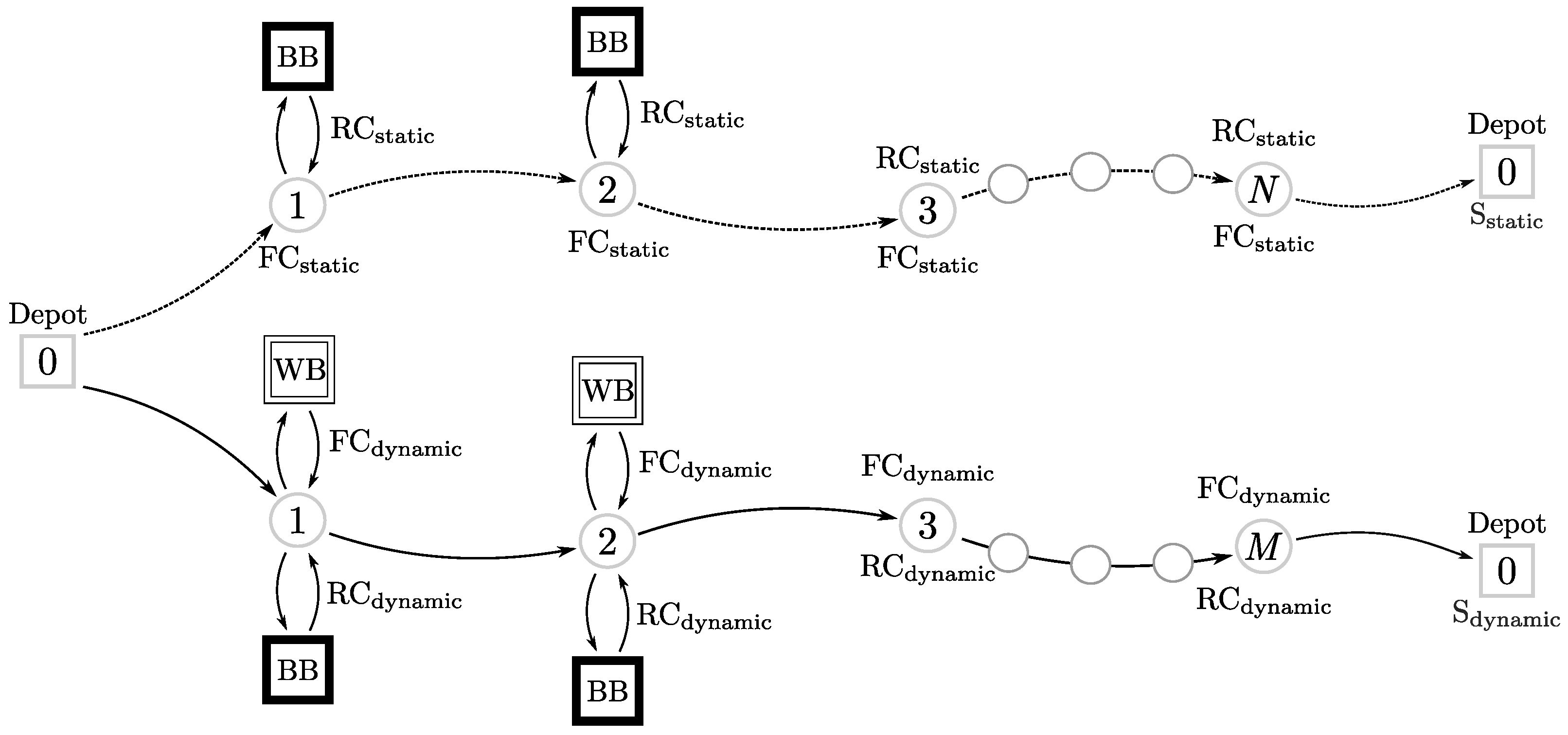
The main challenge of our approach relies on being able to learn from new data (observations) obtained by checking our estimated cost with the real-life cost associated with our routing plan. Thus, we propose a hybrid approach integrating statistical learning [11] into a metaheuristic-based framework [12]. The metaheuristic component constructs new candidate solutions while the statistical learning component, based on the data gathered, makes predictions of the traveling time associated with each edge under the current system status. Some preliminary work can be found in [13,14], which offers a comprehensive review on this hybrid framework and presents it as a novel methodology. However, in their application, both components are not dependent but separate entities combined to solve a VRP where customers’ demands depend on the visiting order. In contrast, in our methodology, both components work together at each step while building solutions. This is done by generating data based on the decisions made so far, which is fed to the statistical learning model to make predictions regarding future decisions. Thus, we create an interdependence of both components to construct high-quality solutions. Figure 1 represents the basic idea behind the learnheuristics methodology applied to the dynamic VRP. In our approach, we will consider a ‘black box’ (BB) and a ‘white box’ (WB). The BB is an emulator of a real-life system that modifies the cost of a route based on its structure. The WB represents the statistical learning model, which aims at predicting the behavior of the BB. Figure 1 illustrates two approaches considering dynamic inputs: (i) the static approach (upper line), where the dynamism is ignored; and (ii) the dynamic approach (solid line) where the WB is used to predict the inputs at each step of the constructive methodology for building a solution. In the static approach, the BB is used to compute the real cost (RC) of the solutions, but no predictions are made. Also in the static approach, the model for the forecasted cost (FC) considers that the cost does not change throughout the construction of the solution. On the contrary, in the dynamic approach, data from the system and the outputs provided by the BB are gathered to generate FCs with the WB. Given a WB able to reproduce the behavior of the BB, we will be able to plan near-optimal routes by considering accurate input estimates. The solutions for the static and the dynamic approaches may be different since the decision-maker receives different information in each case.
In this context, the main contributions of this work are: (i) to describe a more realistic version of the VRP, which includes dynamic traveling times; (ii) to introduce a hybrid solving methodology based on statistical learning techniques and a metaheuristic algorithm; and (iii) to build a set of benchmark instances, which allow other researchers to replicate our computational experiments and/or to compare their methodologies with ours.
The rest of this paper is organized as follows: Section 2 provides a description of the problem addressed. Afterwards, Section 3 reviews related works, considering works on dynamic VRPs, as well as works on hybridizing metaheuristics and statistical learning to deal with combinatorial optimization problems. Section 4 presents the learnheuristics-based methodology proposed to solve the problem. Section 5 explains the computational experiments carried out to illustrate both the problem and the approach, while Section 6 analyzes the results obtained. Finally, Section 7 draws some conclusions and identifies some potential lines for future research.
2. Problem Description
The VRP is a well-known NP-hard problem. Accordingly, metaheuristic solving approaches have been developed to solve large-scale instances in reasonable computing times. Consider a complete and undirected graph , where is a set of nodes composed of a depot 0 and n customers, and E is the set of edges connecting all nodes in V. Each customer i has a positive demand, . Traversing an edge in E has an associated fixed cost . There is a fleet of homogeneous vehicles, each with a capacity Q, with . A solution for this problem is a set of round-trip routes starting at the depot and connecting a set of customers. The total delivery in each route cannot exceed the capacity of each vehicle, Q. All the demands have to be satisfied and a customer may only be visited once. Typically, the objective function minimizes the total distribution costs.
The DVRP that we consider assumes that the costs are , where is the average cost associated with the edge , and S is the current state of the problem. A key aspect is that is unknown, and can only be computed once we have defined a state S. Thus, the costs are neither known in advance nor static. Indeed, they may depend on unpredictable factors (such as accidents) or predictable ones (such as the weather or the congestion level). We build a model (WB) that will estimate the behavior of f in order to generate accurate forecasts regarding the consequences of our decisions. This approach is based on online statistical learning since new data is progressively used to update the model.
For experimental purposes, the BB function f, which is unknown for the solving approach, is defined as:
where is the load of the vehicle at the moment of departure from node i in route k, and are parameters of the model, and is an error term which follows a uniform distribution. We use this model as the BB, and each time the solving approach evaluates one candidate solution, it provides data of a realization (i.e., after completing these routes). The WB is progressively updated and improved with this new data. Notice that Equation (1) represents the real-life (black box) dynamic behavior in our model. Thus, the real cost (e.g., traveling time) associated with traversing an edge is a function of the system status. For experimental purposes, we assume that this real-life cost can be modeled as a linear function of the vehicle load in the traversed edge. Of course, the exact value of this load will depend upon the customers already visited by the vehicle in its assigned route, i.e., these inputs are influenced by the decision variables.
3. Literature Review
The first part of this section reviews recent works that solve a dynamic version of the VRP, while the second part refers to other works that hybridize metaheuristics and statistical learning methods to address combinatorial optimization problems.
3.1. Literature on the DVRP
The first formulation of the dynamic routing problem was proposed by [15] some decades ago. However, it was not until the beginning of this century when the popularity of the DVRP started to increase significantly. Several types of dynamism have been studied through the years. For instance, authors in reference [16] consider dispatch with dynamic velocities. Using a tabu search metaheuristic, these authors improve previous speed models, where the speed of the vehicle is a piecewise continuous function over time and while satisfying the non-passing condition. Similarly, authors in reference [17] work with dynamic velocities based on traffic congestion models. In [18], the authors model future demands with dynamism. Their method predicts a new customer request and plans accordingly in order to satisfy it. The probability of request occurrence is generated from historical data. Later, authors in reference [19] analyze the dynamism coming from the flow of time. Likewise, those in reference [20] study time-varying travel times in vehicle routing. A smoothing and piecewise continuous function is employed to define these travel times, which are known in advance (i.e., before planning the routes). Authors in reference [21] define times relying on a queuing theory model. A hybrid framework is presented in [22], where state space variables are used to predict new demands based on historical data. Another hybrid metaheuristic method can be found in [23]. Their method requires this data to build the model beforehand. For a comprehensive review on the DVRP, the reader is referred to [24]. Although in these versions of the DVRP the inputs are dynamic, in none of them is the dynamism influenced by the decisions of the planner, as it is the case in our paper. Thus, this kind of dynamism remains quite unexplored despite being of high importance in practical routing problems.
3.2. Literature on Metaheuristics and Statistical Learning Hybridization
The hybridization of statistical learning and optimization techniques constitutes an emerging field that has been receiving a lot of attention in recent years. For instance, reference [25] reviews a few works illustrating the potential of hybridizing metaheuristics with mathematical programming, constraint programming, and machine learning. The author concludes that, while there are many works applying optimization to improve data mining techniques, the challenge is in using data mining to help metaheuristics. This issue has been addressed by [26], where the authors identify a few synergies in a short survey. The synergies between operations research and data mining in multi-objective problems are explored in [27]. This work remarks that, while these two fields have a common history, it is still an emerging field with a lot of room for new methodologies. Authors in reference [28] focus on the combination of evolutionary computation techniques with machine learning and present a comprehensive survey. Here, we have discussed some recent and relevant works; for an extended review see [14].
4. Proposed Methodology
This section presents our hybrid approach for solving the DVRP. It is divided into three parts: (i) an overview of the metaheuristic-based framework; (ii) the description of the statistical learning model; and (iii) the hybridization of both methodologies.
4.1. Metaheuristic Algorithm
There are plenty of metaheuristics that may be applied to address the DVRP. We propose a multi-start method [29], which is a highly popular and relatively simple-to-implement metaheuristic with a reduced number of parameters. It proposes to iteratively build solutions from scratch until a stopping criterion is satisfied, and then return the best one. The constructive heuristic of the proposed solving approach for building solutions is the Clarke and Wright’s Savings (CWS) heuristic [30], which is a classical and fast heuristic for the VRP. In particular, the CWS is an iterative method that considers an initial base solution where each customer is served by a dedicated vehicle. Then, the heuristic starts an iterative process where route merges are applied so that vehicles can serve various customers. The merging criterion is based on the concept of savings. Given two customers, a savings value is assigned to the edge connecting them. This savings value represents the savings in cost generated by serving both customers with the same vehicle instead of using a dedicated vehicle for each customer. Thus, a list of edges ranked by their savings can be constructed. This is the so-called savings list. At each iteration of the process, the first edge on the list is taken as a candidate for merging the corresponding routes. There are two conditions that have to be satisfied to accept the merge: (i) the nodes defining the edge are adjacent to the depot; and (ii) the total demand of the customers in the new route does not exceed the capacity of the vehicle. The merging process continues until there are no more edges on the list to be considered, ending the heuristic method. The CWS heuristic usually provides good solutions for small and medium size problem instances [31]. Authors in reference [32] propose an improvement of the CWS heuristic. Their approach, biased randomized CWS (BR-CWS), introduces non-uniform randomness in the selection of edges to be considered from the savings list. While the classical heuristic considers iteratively each edge in the list (which is sorted from the edge with the highest savings to the one with the lowest savings), the BR-CWS algorithm reorders that list with a non-uniform or biased randomness. In particular, a random number is generated from a given probability distribution (either a theoretical or an empirical one). Then, the edge in the position of the random number is selected and deleted from the list of savings, and the merging of the corresponding routes is considered. Afterwards, a new random number is generated and the same steps are applied until the savings list is empty. A skewed probability distribution is required to follow the logic behind the CWS heuristic. In other words, the higher the savings associated with an edge, the higher its probability of being selected. By modifying the greedy behavior of the CWS heuristic, the randomized version may consider more solutions and return a better one. Obviously, building more solutions also means more computational time. However, since the CWS heuristic is fast, the BR-CWS heuristic may build hundreds or thousands of solutions in just a few seconds. Biased randomization techniques have been successfully applied to solve different VRPs [33,34,35,36], arc routing problems [37], and even scheduling problems [38,39,40]. For a complete review on biased-randomization techniques, the reader is referred to [41].
4.2. Statistical Learning Model
Statistical learning tools have been gaining popularity over the last decades. There are plenty of methods to build predictive functions, which estimate the relationship between variables. The nature of the problem analyzed here requires making predictions. In particular, we predict the costs of an edge (dependent variable) for a given state of the problem (predictors), which is needed because the real costs are only revealed after the moment of realization.
It is crucial to select an appropriate method for a specific problem. Each statistical learning method represents a trade-off between performance, interpretability and computing time. Neural networks and support vector machines rank among the best performers due to their high flexibility. However, they also lack interpretability and require long computational times due to all the parameter tuning needed. Moreover, they are prone to overfitting (i.e., the model may capture the noise in the data). Linear regressions, despite being rigid methods, offer great interpretability and are faster to compute. Obviously, they tend to perform better in problems where the relationship between variables–or a transformation of these–is approximately linear.
We choose to employ a multiple linear regression model. As mentioned before, the solving approach relies on the WB, which aims to predict the behavior of the BB. The model is fed with the variables: load, number of nodes visited in a route, number of routes, and the capacity of the vehicle. Using multiple regression analysis [42], and after analyzing the correlation matrix and the individual p-values for the different variables, we found that the relevant variables are the load and the capacity of the vehicle. Thus, we build a linear regression model with just the load and the capacity of the vehicle, reducing the usage of memory and the computational time required.
4.3. Hybridization of the Metaheuristic Algorithm and the Statistical Learning Model
The pseudo-code of our approach for building a single solution is shown in Algorithm 1 and explained next. In the (static) VRP, the savings list is generated once at the beginning of the execution, and it remains constant throughout the resolution. The savings associated with an edge is the benefit from merging the corresponding routes. When two routes are merged, the total cost of the new route cannot be greater than the sum of the individual separated routes (i.e., the saving cannot be negative when the cost is based on the Euclidean-distance metric due to the triangle inequality). This statement is no longer true in general for dynamic inputs due to the change of the state of the problem. Thus, the savings must be computed with the total cost of the routes. In the DVRP, we know the current state of the problem and, as a consequence, the cost of the two separate routes to merge. However, we do not know the total cost of the merged route before actually merging it. Thus, it is needed to predict this cost based on historical data, and then recompute the savings (see pseudo-code of Algorithm 2).
The static approach for this problem does not present this nuance because the cost of a route is always known, while in our case it is only revealed once the merge is done. A key difference with respect to the static approach is the update of the savings list by means of the predictive model at each new state due to the dynamic nature of the problem. The hybridization of the metaheuristic and the statistical learning model is necessary to perform the task of keeping the list updated when new information is available. Generally, training a statistical learning model is an expensive task. The choice of implementing a multiple linear regression model was favored mainly for its fast execution times. Notice that the metaheuristic-based framework would not change if another statistical learning model was considered.
| Algorithm 1 Procedure to build a DVRP solution using the BR-CWS heuristic. |
| 1: procedure BuildDVRPsol(inputs) 2: solution ← generateBaseSolution(inputs) ▹inputs: coordinates, demands and vehicles’ capacity 3: savings ← computeSavings(solution, whiteBox) ▹ edges list decreasingly sorted by savings 4: while (savings is not empty) do 5: index ←generate random number ▹ given probability distribution 6: edge ← get edge from savings by index 7: savings ← delete edge from savings 8: if (mergeFeasible(edge)) then 9: route ← emptyRoute 10: route ← mergeRoutes(edge, solution) 11: realCost ← blackBox.getRealCost(route) 12: solution.update(realCost) ▹ update solution with the real cost of the route 13: whiteBox.update(route, realCost) ▹ update White Box 14: savings ← computeSavings(solution, whiteBox) ▹ update savings 15: end if 16: end while 17: return 18: end procedure |
| Algorithm 2 Procedure to compute the savings list. |
| 1: procedure ComputeSavings(solution, whiteBox) 2: savings ← emptyList 3: exteriorNodes ← getExteriorNodes(nodes) 4: for to exteriorNodes.size do 5: for to exteriorNodes.size do 6: iRoute ← getRoute(exteriorNodes(i) 7: jRoute ← getRoute(exteriorNodes(j)) 8: mergedRoute ← mergeRoutes(iRoute, jRoute) 9: iRealCost ← getCost(iRoute) ▹ Black Box 10: jRealCost ← getCost(jRoute) 11: mergedPredictedCost ← whiteBox.predictCost(mergedRoute, solution) ▹ Based on the state of the problem 12: routeSavings ← iRealCost + jRealCost - mergedPredictedCost 13: add routeSavings to savings 14: end for 15: end for 16: savings.sort ▹ Sort in descending order 17: return savings 18: end procedure |
5. Computational Experiments
This section describes the computational experiments carried out to illustrate both the problem and the solving methodology, comparing different approaches. After introducing the experiments, we describe the instances and the parameters required, and summarize the results. A comprehensive analysis of the results is shown in the next section.
The algorithm described in this paper has been implemented as a Java application, and the Apache Commons Mathematics Library has been used to build the linear regression model. A standard personal computer, Intel® Core™ i5-8250U @ GHz and 8 GB of RAM has been used to execute the application.
The experiments compare two approaches to deal with the DVRP: (i) the static approach where the FCs are the cost of the edge using the Euclidean distance and do not change throughout the construction of the solution; and (ii) the dynamic approach where the FCs are predicted by the WB based on data from the BB. We compare the FC and the RC obtained with the static approach (called SFC and SRC, respectively) with the FC and the RC obtained with the dynamic approach (DFC and DRC, respectively). The comparison is done by computing the percentage gaps among them relative to the DRC. One should expect that ignoring the dynamism of the system will lead the static approach to generate suboptimal solutions. Thus, we expect the SRC to be greater than the DRC, at least on average. In addition, the SFC should be smaller than the DRC on the average, since the BB usually increases the cost of the routes. Lastly, one should expect the DFC to be similar in value to the DRC, since the WB should be able to make accurate predictions on the corrections of the BB.
5.1. Description of Instances
The set of instances that we employ to test our approach is a natural extension of the classical benchmark instances for the VRP, which are available at http://vrp.atd-lab.inf.puc-rio.br/index.php/en/. This site provides a detailed description of each instance as well as a tool to visualize the distribution of the nodes. Each instance describes the capacity of the vehicle, the coordinates of each node and also its demand. Instances from different sets (A, B, E, M, F, and P) have been selected for the experiments. Instances with less than 24 nodes have been discarded because they can be easily solved by using exact methods. Instances from the sets A, E, and P have a homogeneously dispersed configuration of nodes, where the depot may be at the center or at any other location. The set F and some instances of E have a more heterogeneous density of nodes. Otherwise, sets B and M have several clusters of nodes and, in some cases, the depot belongs to one cluster. The name of the instances considered are listed along with the number of nodes and the capacity of the vehicles in the first columns of Table 1.
In our experiments, these basic instances have been extended by incorporating different levels of dynamism in the traveling times. The specific level of dynamism employed is a design parameter. Hence, we should expect our results to converge to the best-known solutions for the original instances whenever the level of dynamism of travel times converges to zero. On the contrary, as this level grows, our results should diverge from the classical ones, and using the near-optimal solutions for the non-dynamic version in the dynamic scenario should lead to suboptimal results.
5.2. Parameters of the Algorithm and the Tests
Our methodology has a few parameters that need to be set before executing the algorithm. As in any other metaheuristic, the choice of these parameters could eventually affect the performance of our algorithm. First, the model for the BB has three parameters: the regression parameters , and the error term (see Equation (1)). Our approach to fix them consists in: (i) the BB should give corrections of reasonable order of magnitude; and (ii) this order of magnitude should be the same for all instances. Considering these two statements, the BB is modeled as:
with C being the capacity of the vehicle. In this way, . Let us consider the extreme cases:
With this model, the corrections are bounded to times the average cost of the edge for all instances. The extreme cases here are reasonable as the corrections do not change the average cost drastically. Using the capacity of the vehicle as a parameter allows us to generalize the corrections for all the instances, thus avoiding possible difficulties in using a general model for any type of problem configuration. The error term is set in a range , which is about two orders of magnitude smaller than the order of the corrections. As discussed in [41], one effective way to transform a deterministic heuristic into a biased-randomized algorithm is by using a geometric probability distribution. This allows for assigning, during the solution-construction process, higher probabilities of being selected to those movements that are more promising according to the heuristic criterion. The geometric distribution has only one parameter . Values of p closer to 1 reproduce the greedy behavior of the original heuristic, while values of p closer to 0 represent a uniform selection of candidates, which ignores the logic behind the heuristic. Values in between these extremes allow for considering this logic while, at the same time, do not follow a greedy deterministic behavior. After some initial tests, we noticed that the BR-CWS probabilistic algorithm was able to provide high-quality solutions when using values of p inside the interval .
In the iterative procedure, there is a lot of data generated by the BB. There is no need to use all of it to compute a predictive model that estimates, in an accurate way, the BB. In the preliminary tests we realized, it was observed that only around 500 instances of data were needed to build an accurate model. In this way, the computational time is reduced by not updating the predictive model at every iteration of the algorithm.
As is usual in the literature, the algorithm has been executed several times for each approach, each time with a different seed for the pseudo-random number generator. The same 30 seeds have been employed for both approaches. Only the best solutions have been stored. This reduces the options of obtaining a poor solution due to the effect of the seed [43].
5.3. Computational Results
The results of our experiments comparing the static and dynamic approaches are summarized in Table 1. It is structured as follows. The first three columns refer to the instance considered (name, number of nodes, and capacity of the vehicle). The next four columns describe the forecasted and the real costs for both approaches. Then, the number of routes for the solutions of each approach is revealed. Finally, the last three columns represent the gaps with respect to the DRC. The average values of each gap are shown in the last row.
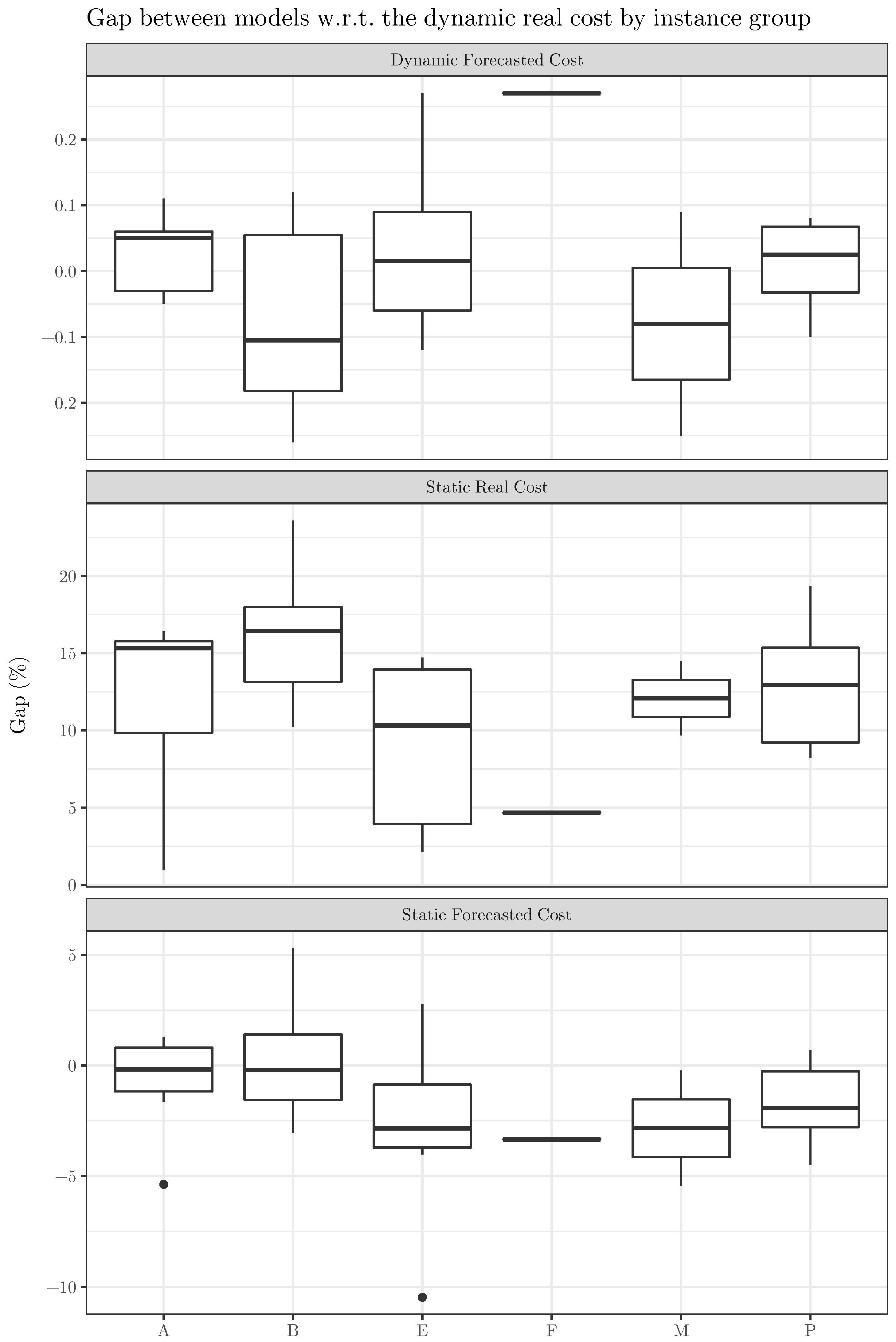
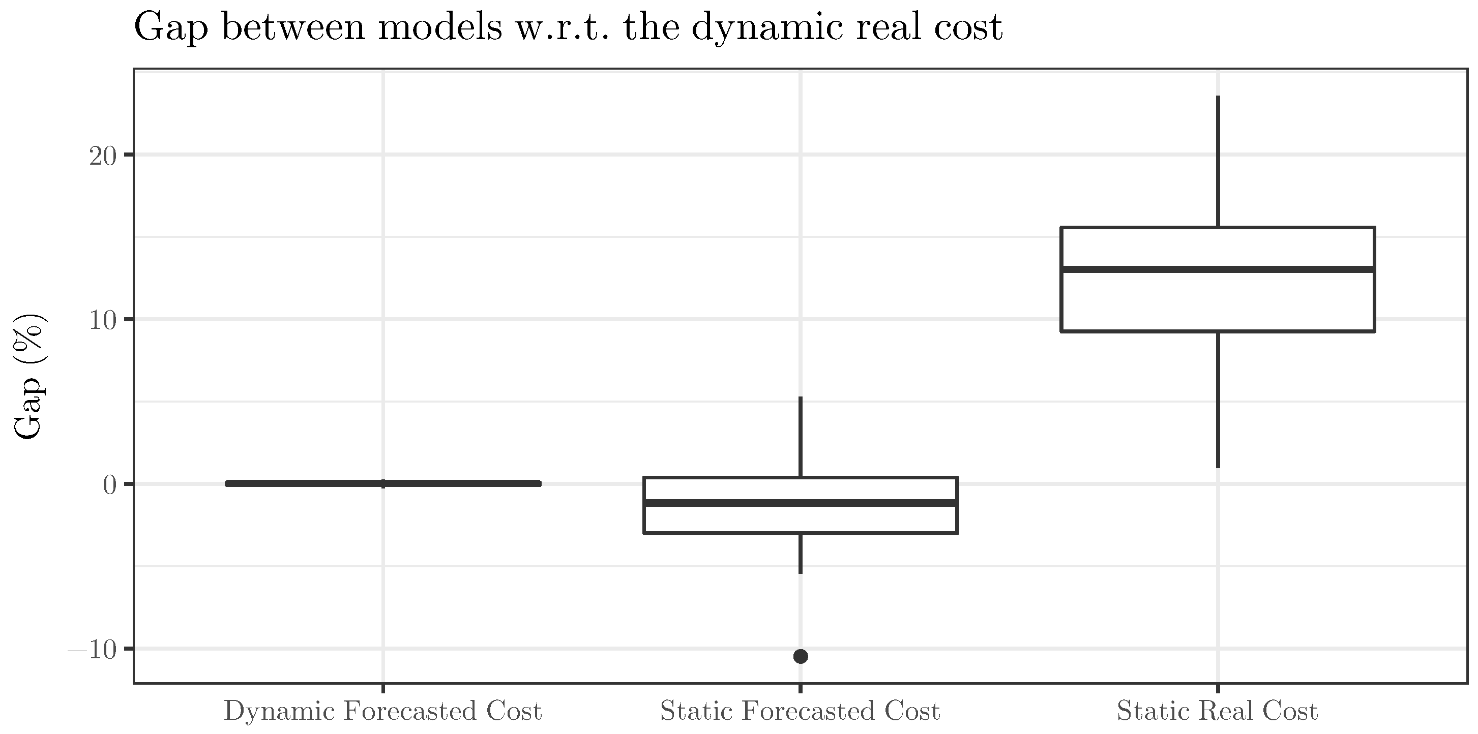
Figure 2 and Figure 3 display the gaps using multiple boxplots. In particular, the first figure shows boxplots of each gap by instance set. In contrast, the second figure aggregates the gaps among all the sets and uses the same scale to represent the three resulting boxplots, which helps us to easily compare their magnitude.
6. Analysis of the Results
The columns of gaps in Table 1 show the relative differences between the best solutions obtained with the static and dynamic approaches. The positive gaps between SRC and DRC proves the importance of considering the intrinsic dynamism of the system. Indeed, the maximum gap reaches a value of 23.58%, while the average gap is around . All the gaps are strictly positive, thus the static approach does not outperform the dynamic one in any instance. Regarding the gaps between DFC and DRC, the amount is lower: the greater gap in terms of absolute values is 0.26%, and the mean is 0.00%. This is due to the fast learning of the linear regression model, which can be explained due to the fact that the BB model is linear and has a relatively small error term. Finally, there are positive and negative gaps between SFC and DRC, but SFC is, on average, lower than DRC. Thus, when the dynamism is not considered, the forecast of real costs tends to be optimistic, misleading the planner. It is worth remarking that, while SFC and SRC are similar in some instances, the routes of those solutions are different. The planner may be deceived into thinking that ignoring dynamism leads to a solution with a similar performance to that of the optimal solution; however, once those routes are completed, SRC is greater than SFC.
Figure 2 represents graphically the gaps considering the different instance sets. Regarding the gaps between DFC and DRC (first raw of boxplots), we observe that the groups of instances have different distributions of gaps, but they tend to be relatively small. The distributions are relatively symmetric, except for sets A (negative skew) and F (no variability at all). There are no outliers. We focus now on the gaps between SRC and DRC. They range between almost 0% and 25%. The boxplots per group of instances share some similarities with the previous ones: symmetry except for sets A (positive skew) and F (no variability at all), there are no outliers, and the variability (either total range and interquartile range) depends on the set (higher for set E and lower for set M, for example). Finally, the last row displays the boxplot of the gaps between SFC and DR. They range between −10% and 5%, approximately. There are only two outliers, and the variability is also group-dependent: for sets B and E is higher than for F. There is also symmetry in this case. Since there is not any pair of sets with a similar distribution of gaps, it is difficult to link the main differences of the sets (described in Section 5.1) to the boxplots.
Figure 3 aggregates the gaps by sets, and displays them using a unique scale, thus allowing a direct comparison. The gaps range between −10% and 25%, approximately. The boxplot for the gaps between DFC and DRC is a single line. Regarding the gaps between SFC and DRC, the boxplot represents a symmetric distribution with a negative outlier and a slightly negative median. Finally, the boxplot for the gaps between SRC and DRC shows a higher variability but is also symmetric. The first and third quartiles are close to 10% and 15%, respectively.
7. Conclusions
With an increasing concern for the environment, it is becoming a key aspect for governments to boost smart and sustainable transportation systems. While the literature on rich vehicle routing problems (VRPs) is extensive, some issues remain to be addressed. For example, most works assume that the traveling times between pairs of nodes are both known in advance and static. In contrast, this paper has focused on the dynamism characterizing many real-world routing applications, where traveling times are dynamic in nature.
Taking into account the high number of factors that might affect the traveling time (from accidents to the weather), we introduce the VRP with dynamic traveling times. In particular, these times vary dynamically as the routing plan is being generated. Therefore, they need to be re-evaluated dynamically during the optimization process. As far as we know, this is the first work addressing this version of the dynamic VRP. In order to deal with this problem, a hybrid solving approach has been presented. Our approach integrates a statistical learning technique into a multi-start framework. A comprehensive set of computational experiments have been carried out to quantify the differences between ignoring or not the dynamism in traveling times among many realistic scenarios. The results show an average gap around 12.02%, with all gaps being positive (i.e., it always pays off to take this dynamism into account while designing the routing plan).
Several lines of research stem from this work. For instance, we have employed a linear model as an emulator of a real system that provides data for building/updating our model. Thus, analyzing the convenience of building a more sophisticated emulator would be an interesting research line. If the function was not linear, it could make sense to apply and compare the performance of different statistical learning techniques. In case of requiring time-consuming techniques, the use of a distributed computing system could be tested. Finally, it would be interesting to model richer VRPs (heterogeneous fleet, multiple depots, etc) considering also dynamic traveling times influenced by the manager decisions.
Author Contributions
Conceptualization, Formal Analysis, Supervision, and Writing, A.A.J. and I.S.; Software Implementation and Validation, Q.A.
Funding
This research received no external funding.
Acknowledgments
This work has been partially carried out in the context of the Erasmus+ program (2017-1-ES01-KA103-036672).
Conflicts of Interest
The authors declare no conflict of interest.
References
- Demir, E.; Bektaş, T.; Laporte, G. A review of recent research on green road freight transportation. Eur. J. Oper. Res. 2014, 237, 775–793. [Google Scholar] [CrossRef] [Green Version]
- Reyes, L.; Calvet, L.; Juan, A.; Faulin, J.; Bove, L. Sustainable urban freight transport: A multi-depot vehicle routing problem considering different cost dimensions. J. Heuristics 2018. [Google Scholar] [CrossRef]
- Faulin, J.; Grasman, S.; Juan, A.; Hirsch, P. Sustainable Transportation and Smart Logistics: Decision-Making Models and Solutions; Elsevier: Amsterdam, The Netherlands, 2018. [Google Scholar]
- Juan, A.A.; Mendez, C.A.; Faulin, J.; de Armas, J.; Grasman, S.E. Electric vehicles in logistics and transportation: A survey on emerging environmental, strategic, and operational challenges. Energies 2016, 9, 86. [Google Scholar] [CrossRef]
- Demartini, M.; Pinna, C.; Aliakbarian, B.; Tonelli, F.; Terzi, S. Soft Drink Supply Chain Sustainability: A Case Based Approach to Identify and Explain Best Practices and Key Performance Indicators. Sustainability 2018, 10, 3540. [Google Scholar] [CrossRef]
- Demartini, M.; Orlandi, I.; Tonelli, F.; Anguitta, D. A manufacturing value modeling methodology (MVMM): A value mapping and assessment framework for sustainable manufacturing. In Proceedings of the International Conference on Sustainable Design and Manufacturing, Bologna, Italy, 26–28 April 2017; Springer: Berlin, Germany, 2017; pp. 98–108. [Google Scholar]
- Eurostat. Sustainable Development in the European Union: 2015 Monitoring Report of the EU Sustainable Development Strategy; European Union: Brussels, Belgium, 2015; pp. 1–351. [Google Scholar]
- Cáceres-Cruz, J.; Arias, P.; Guimarans, D.; Riera, D.; Juan, A.A. Rich vehicle routing problem: A survey. ACM Comput. Surv. (CSUR) 2015, 47, 32. [Google Scholar] [CrossRef]
- Cassettari, L.; Demartini, M.; Mosca, R.; Revetria, R.; Tonelli, F. A Multi-Stage Algorithm for a Capacitated Vehicle Routing Problem with Time Constraints. Algorithms 2018, 11, 69. [Google Scholar] [CrossRef]
- Dutkiewicz, L.; Kucharska, E.; Raczka, K.; Grobler-Debska, K. ST method-based algorithm for the supply routes for multilocation companies problem. In Knowledge, Information and Creativity Support Systems: Recent Trends, Advances and Solutions; Springer: Berlin, Germany, 2016; pp. 123–135. [Google Scholar]
- Friedman, J.; Hastie, T.; Tibshirani, R. The Elements of Statistical Learning; Springer Series in Statistics; Springer: New York, NY, USA, 2001; Volume 1. [Google Scholar]
- Gendreau, M.; Potvin, J.Y. Handbook of Metaheuristics; Springer: Berlin, Germany, 2010; Volume 2. [Google Scholar]
- Calvet, L.; Ferrer, A.; Gomes, M.I.; Juan, A.A.; Masip, D. Combining statistical learning with metaheuristics for the multi-depot vehicle routing problem with market segmentation. Comput. Ind. Eng. 2016, 94, 93–104. [Google Scholar] [CrossRef]
- Calvet, L.; Armas, J.D.; Masip, D.; Juan, A.A. Learnheuristics: Hybridizing metaheuristics with machine learning for optimization with dynamic inputs. Open Math. 2017, 15, 261–280. [Google Scholar] [CrossRef]
- Wilson, N.; Sussman, J.; Wong, H. Scheduling Algorithms for a Dial-a-Ride System; PB 201 808; Massachusetts Institute of Technology, Urban Systems Laboratory: Cambridge, MA, USA, 1971. [Google Scholar]
- Ichoua, S.; Gendreau, M.; Potvin, J.Y. Vehicle dispatching with time-dependent travel times. Eur. J. Oper. Res. 2003, 144, 379–396. [Google Scholar] [CrossRef]
- Kok, A.L.; Hans, E.W.; Schutten, J.M. Vehicle routing under time-dependent travel times: The impact of congestion avoidance. Comput. Oper. Res. 2012, 39, 910–918. [Google Scholar] [CrossRef] [Green Version]
- Ichoua, S.; Gendreau, M.; Potvin, J.Y. Exploiting Knowledge About Future Demands for Real-Time Vehicle Dispatching. Transp. Sci. 2006, 40, 211–225. [Google Scholar] [CrossRef] [Green Version]
- Pillac, V.; Guéret, C.; Medaglia, A.L. An event-driven optimization framework for dynamic vehicle routing. Decis. Support Syst. 2012, 54, 414–423. [Google Scholar] [CrossRef] [Green Version]
- Fleischmann, B.; Gietz, M.; Gnutzmann, S. Time-Varying Travel Times in Vehicle Routing. Transp. Sci. 2004, 38, 160–173. [Google Scholar] [CrossRef]
- Van Woensel, T.; Kerbache, L.; Peremans, H.; Vandaele, N. Vehicle routing with dynamic travel times: A queueing approach. Eur. J. Oper. Res. 2008, 186, 990–1007. [Google Scholar] [CrossRef]
- Sáez, D.; Cortés, C.E.; Núñez, A. Hybrid adaptive predictive control for the multi-vehicle dynamic pick-up and delivery problem based on genetic algorithms and fuzzy clustering. Comput. Oper. Res. 2008, 35, 3412–3438. [Google Scholar] [CrossRef]
- Avci, M.; Topaloglu, S. A hybrid metaheuristic algorithm for heterogeneous vehicle routing problem with simultaneous pickup and delivery. Expert Syst. Appl. 2016, 53, 160–171. [Google Scholar] [CrossRef]
- Psaraftis, H.N.; Wen, M.; Kontovas, C.A. Dynamic Vehicle Routing Problems: Three Decades and Counting. Networks 2016, 67, 3–31. [Google Scholar] [CrossRef]
- Talbi, E.G. Combining metaheuristics with mathematical programming, constraint programming and machine learning. Ann. Oper. Res. 2016, 240, 171–215. [Google Scholar] [CrossRef]
- Jourdan, L.; Dhaenens, C.; Talbi, E.G. Using Datamining Techniques to Help Metaheuristics: A Short Survey; Hybrid Metaheuristics; Springer: Berlin, Heidelberg, 2006; pp. 57–69. [Google Scholar]
- Corne, D.; Dhaenens, C.; Jourdan, L. Synergies between operations research and data mining: The emerging use of multi-objective approaches. Eur. J. Oper. Res. 2012, 221, 469–479. [Google Scholar] [CrossRef]
- Zhang, J.; Zhang, Z.H.; Lin, Y.; Chen, N.; Gong, Y.J.; Zhong, J.H.; Chung, H.S.; Li, Y.; Shi, Y.H. Evolutionary computation meets machine learning: A survey. IEEE Computat. Intell. Mag. 2011, 6, 68–75. [Google Scholar] [CrossRef]
- Martí, R.; Lozano, J.A.; Mendiburu, A.; Hernando, L. Multi-start methods. In Handbook of Heuristics; Springer: Berlim, Germany, 2016; pp. 1–21. [Google Scholar]
- Clarke, G.; Wright, J.W. Scheduling of Vehicles from a Central Depot to a Number of Delivery Points. Oper. Res. 1964, 12, 568–581. [Google Scholar] [CrossRef]
- Faulin, J.; Juan, A.A. The ALGACEA-1 method for the capacitated vehicle routing problem. Int. Trans. Oper. Res. 2008, 15, 599–621. [Google Scholar] [CrossRef]
- Juan, A.A.; Faulin, J.; Ruiz, R.; Barrios, B.; Caballé, S. The SR-GCWS hybrid algorithm for solving the capacitated vehicle routing problem. Appl. Soft Comput. 2010, 10, 215–224. [Google Scholar] [CrossRef]
- Dominguez, O.; Juan, A.A.; Faulin, J. A biased-randomized algorithm for the two-dimensional vehicle routing problem with and without item rotations. Int. Trans. Oper. Res. 2014, 21, 375–398. [Google Scholar] [CrossRef]
- Juan, A.A.; Pascual, I.; Guimarans, D.; Barrios, B. Combining biased randomization with iterated local search for solving the multidepot vehicle routing problem. Int. Trans. Oper. Res. 2015, 22, 647–667. [Google Scholar] [CrossRef]
- Dominguez, O.; Juan, A.A.; Barrios, B.; Faulin, J.; Agustin, A. Using biased randomization for solving the two-dimensional loading vehicle routing problem with heterogeneous fleet. Ann. Oper. Res. 2016, 236, 383–404. [Google Scholar] [CrossRef]
- Dominguez, O.; Guimarans, D.; Juan, A.A.; de la Nuez, I. A biased-randomised large neighbourhood search for the two-dimensional vehicle routing problem with backhauls. Eur. J. Oper. Res. 2016, 255, 442–462. [Google Scholar] [CrossRef]
- de Armas, J.; Ferrer, A.; Juan, A.A.; Lalla-Ruiz, E. Modeling and solving the non-smooth arc routing problem with realistic soft constraints. Expert Syst. Appl. 2018, 98, 205–220. [Google Scholar] [CrossRef]
- Juan, A.A.; Lourenço, H.R.; Mateo, M.; Luo, R.; Castella, Q. Using iterated local search for solving the flow-shop problem: Parallelization, parametrization, and randomization issues. Int. Trans. Oper. Res. 2014, 21, 103–126. [Google Scholar] [CrossRef]
- Ferrer, A.; Guimarans, D.; Ramalhinho, H.; Juan, A.A. A BRILS metaheuristic for non-smooth flow-shop problems with failure-risk costs. Expert Syst. Appl. 2016, 44, 177–186. [Google Scholar] [CrossRef] [Green Version]
- Martin, S.; Ouelhadj, D.; Beullens, P.; Ozcan, E.; Juan, A.A.; Burke, E.K. A multi-agent based cooperative approach to scheduling and routing. Eur. J. Oper. Res. 2016, 254, 169–178. [Google Scholar] [CrossRef] [Green Version]
- Grasas, A.; Juan, A.A.; Faulin, J.; de Armas, J.; Ramalhinho, H. Biased Randomization of Heuristics using Skewed Probability Distributions: A survey and some applications. Comput. Ind. Eng. 2017, 110, 216–228. [Google Scholar] [CrossRef]
- Keith, T.Z. Multiple Regression and Beyond: An Introduction to Multiple Regression and Structural Equation Modeling; Routledge: Abingdon-on-Thames, UK, 2014. [Google Scholar]
- Czarn, A.; MacNish, C.; Vijayan, K.; Turlach, B.; Gupta, R. Statistical exploratory analysis of genetic algorithms. IEEE Trans. Evolut. Comput. 2004, 8, 405–421. [Google Scholar] [CrossRef]
Figure 1.
Diagram of the learnheuristics methodology applied to construct a single solution for the DVRP.
Figure 1.
Diagram of the learnheuristics methodology applied to construct a single solution for the DVRP.

Figure 2.
Multiple boxplots comparing the gaps of the different costs relative to the DRC by instance set with a uniformly distributed error term .
Figure 2.
Multiple boxplots comparing the gaps of the different costs relative to the DRC by instance set with a uniformly distributed error term .

Figure 3.
Multiple boxplots comparing the gaps of the different costs relative to the DRC with a uniformly distributed error term .
Figure 3.
Multiple boxplots comparing the gaps of the different costs relative to the DRC with a uniformly distributed error term .


Table 1.
Results for the static and dynamic approaches with a uniformly distributed error term .
| Instances | Cost | # Routes | Gapw.r.t.DRC (%) | ||||||||
|---|---|---|---|---|---|---|---|---|---|---|---|
| Name | # Nodes | vCap | DFC | DRC | SRC | SFC | Dynamic | Static | DFC | SRC | SFC |
| A-n32-k5 | 35 | 100 | 864.04 | 863.05 | 871.49 | 816.73 | 5 | 5 | 0.11 | 0.98 | −5.37 |
| A-n38-k5 | 41 | 100 | 749.47 | 749.08 | 866.13 | 756.09 | 5 | 6 | 0.05 | 15.63 | 0.94 |
| A-n55-k9 | 62 | 100 | 1096.38 | 1096.97 | 1212.64 | 1111.01 | 9 | 9 | −0.05 | 10.54 | 1.28 |
| A-n60-k9 | 67 | 100 | 1405.68 | 1404.75 | 1532.85 | 1381.52 | 9 | 9 | 0.07 | 9.12 | −1.65 |
| A-n61-k9 | 69 | 100 | 1090.09 | 1089.57 | 1256.55 | 1096.9 | 10 | 10 | 0.05 | 15.33 | 0.67 |
| A-n65-k9 | 72 | 100 | 1255.78 | 1256.14 | 1455.82 | 1247.41 | 10 | 10 | −0.03 | 15.90 | −0.69 |
| A-n80-k10 | 88 | 100 | 1831.57 | 1832.1 | 2133.16 | 1828.91 | 10 | 10 | −0.03 | 16.43 | −0.17 |
| B-n35-k5 | 38 | 100 | 1039.05 | 1040.42 | 1215.04 | 1008.91 | 5 | 5 | −0.13 | 16.78 | −3.03 |
| B-n50-k7 | 55 | 100 | 758.91 | 758.12 | 880.08 | 751.18 | 7 | 7 | 0.10 | 16.09 | −0.92 |
| B-n52-k7 | 57 | 100 | 748.98 | 750.9 | 842.1 | 763.72 | 7 | 7 | −0.26 | 12.15 | 1.71 |
| B-n64-k9 | 72 | 100 | 931.49 | 930.4 | 1025.43 | 913.85 | 10 | 10 | 0.12 | 10.21 | −1.78 |
| B-n67-k10 | 75 | 100 | 1039.52 | 1040.37 | 1285.71 | 1095.47 | 10 | 11 | -0.08 | 23.58 | 5.30 |
| B-n78-k10 | 86 | 100 | 1270.07 | 1272.61 | 1506.71 | 1278.83 | 10 | 10 | -0.20 | 18.40 | 0.49 |
| E-n101-k14 | 113 | 112 | 1156.23 | 1155.55 | 1316.35 | 1143.58 | 14 | 14 | 0.06 | 13.92 | −1.04 |
| E-n22-k4 | 24 | 6000 | 378.47 | 378.27 | 431.31 | 388.77 | 4 | 4 | 0.05 | 14.02 | 2.78 |
| E-n23-k3 | 24 | 4500 | 641.18 | 639.43 | 653.12 | 572.47 | 3 | 3 | 0.27 | 2.14 | −10.47 |
| E-n30-k3 | 32 | 4500 | 527.92 | 527 | 547.88 | 512.14 | 4 | 4 | 0.17 | 3.96 | −2.82 |
| E-n33-k4 | 35 | 8000 | 875.96 | 876.15 | 910.05 | 844.53 | 4 | 4 | −0.02 | 3.87 | −3.61 |
| E-n51-k5 | 54 | 160 | 575.43 | 575.67 | 631.93 | 573.68 | 5 | 6 | −0.04 | 9.77 | −0.35 |
| E-n76-k10 | 84 | 140 | 916.5 | 917.56 | 1017.11 | 880.7 | 11 | 11 | −0.12 | 10.85 | −4.02 |
| E-n76-k14 | 89 | 100 | 1093.28 | 1094.58 | 1255.58 | 1063.17 | 15 | 15 | -0.12 | 14.71 | −2.87 |
| F-n135-k7 | 140 | 2210 | 1258.53 | 1255.19 | 1313.82 | 1213.29 | 7 | 7 | 0.27 | 4.67 | −3.34 |
| M-n101-k10 | 109 | 200 | 896.75 | 895.96 | 1025.6 | 893.89 | 10 | 10 | 0.09 | 14.47 | −0.23 |
| M-n200-k16 | 215 | 200 | 1454.7 | 1458.34 | 1599.36 | 1379.05 | 17 | 17 | −0.25 | 9.67 | −5.44 |
| P-n22-k8 | 29 | 3000 | 606.91 | 606.77 | 659.59 | 589.39 | 9 | 9 | 0.02 | 8.71 | −2.86 |
| P-n40-k5 | 43 | 140 | 514.3 | 514.17 | 556.51 | 501.05 | 5 | 5 | 0.03 | 8.23 | −2.55 |
| P-n50-k10 | 59 | 100 | 728.22 | 727.61 | 839.86 | 718.37 | 11 | 11 | 0.08 | 15.43 | −1.27 |
| P-n55-k15 | 70 | 70 | 974.68 | 975.69 | 1164.2 | 982.59 | 16 | 17 | -0.10 | 19.32 | 0.71 |
| P-n65-k10 | 73 | 130 | 871.76 | 871.1 | 964.59 | 832.12 | 10 | 10 | 0.08 | 10.73 | −4.47 |
| P-n70-k10 | 79 | 135 | 884.76 | 885.17 | 1018.95 | 885.85 | 11 | 11 | -0.05 | 15.11 | 0.08 |
| Averages | 0.00 | 12.02 | −1.25 | ||||||||
© 2018 by the authors. Licensee MDPI, Basel, Switzerland. This article is an open access article distributed under the terms and conditions of the Creative Commons Attribution (CC BY) license (http://creativecommons.org/licenses/by/4.0/).
Share and Cite
MDPI and ACS Style
Arnau, Q.; Juan, A.A.; Serra, I. On the Use of Learnheuristics in Vehicle Routing Optimization Problems with Dynamic Inputs. Algorithms 2018, 11, 208. https://doi.org/10.3390/a11120208
AMA Style
Arnau Q, Juan AA, Serra I. On the Use of Learnheuristics in Vehicle Routing Optimization Problems with Dynamic Inputs. Algorithms. 2018; 11(12):208. https://doi.org/10.3390/a11120208
Chicago/Turabian StyleArnau, Quim, Angel A. Juan, and Isabel Serra. 2018. "On the Use of Learnheuristics in Vehicle Routing Optimization Problems with Dynamic Inputs" Algorithms 11, no. 12: 208. https://doi.org/10.3390/a11120208
Note that from the first issue of 2016, this journal uses article numbers instead of page numbers. See further details here.