Mapping the Daily Rainfall over an Ungauged Tropical Micro-Watershed: A Downscaling Algorithm Using GPM Data
by
 and
and
Mohd. Rizaludin Mahmud
1,2,*, 
Aina Afifah Mohd Yusof
2,
Mohd Nadzri Mohd Reba
1,2 and
Mazlan Hashim
1,2 1
Geoscience & Digital Earth Centre, Research Institute for Sustainable Environment, Universiti Teknologi Malaysia, Johor Bharu, Johor 81310, Malaysia
2
Deptartment of Geoinformation, Faculty of Built Environment & Surveying, Universiti Teknologi Malaysia, Johor Bharu, Johor 81310, Malaysia
*
Author to whom correspondence should be addressed.
Water 2020, 12(6), 1661; https://doi.org/10.3390/w12061661
Submission received: 19 April 2020
/
Revised: 3 June 2020
/
Accepted: 8 June 2020
/
Published: 10 June 2020
(This article belongs to the Special Issue Modelling Precipitation in Space and Time)
Abstract
:In this study, half-hourly Global Precipitation Mission (GPM) satellite precipitation data were downscaled to produce high-resolution daily rainfall data for tropical coastal micro-watersheds (100–1000 ha) without gauges or with rainfall data conflicts. Currently, daily-scale satellite rainfall downscaling techniques rely on rain gauge data as corrective and controlling factors, making them impractical for ungauged watersheds or watersheds with rainfall data conflicts. Therefore, we used high-resolution local orographic and vertical velocity data as proxies to downscale half-hourly GPM precipitation data (0.1°) to high-resolution daily rainfall data (0.02°). The overall quality of the downscaled product was similar to or better than the quality of the raw GPM data. The downscaled rainfall dataset improved the accuracy of rainfall estimates on the ground, with lower error relative to measured rain gauge data. The average error was reduced from 41 to 27 mm/d and from 16 to 12 mm/d during the wet and dry seasons, respectively. Estimates of localized rainfall patterns were improved from 38% to 73%. The results of this study will be useful for production of high-resolution satellite precipitation data in ungauged tropical micro-watersheds.
1. Introduction
Daily rainfall is a critical variable used to characterize hydrological dynamics in tropical catchments. In Southeast Asia, many operational and productive micro-watersheds are relatively small (<16 km²) [1,2,3], but are utilized for water supply, irrigation, and hydroelectric power. Despite their small size, these micro-watersheds exhibit high spatiotemporal variability in rainfall patterns [4,5], including extreme rainfall events that release large volumes of water within a short duration [6,7]. Rainfall intensity and distribution vary at short distances in micro-watersheds (~1 km). Additionally, coastal tropical watersheds are influenced by convective processes that determine cloud formation, as well as interactions between seasonal winds from the Asian Monsoon and local topography and geomorphology.
Most micro-watersheds in Southeast Asia have rainfall data conflicts, which are characterized by one or more of the following problems: lack of rain gauges, sparse rain gauge coverage, missing rain gauge data, inefficient data sharing policies, or ineffective data management [8]. These conflicts often cause ineffective watershed management, which can lead in turn to water resource, flood, water-borne disaster, and biodiversity management failures. Satellite precipitation data can be used as a support for ungauged sub-catchments or those with data conflicts; however, their use is constrained by spatial resolution and sub-catchment size limitations. The coarse grid size of satellite data is a major constraint, whereby satellite precipitation data are unable to effectively represent spatial rainfall distribution at the sub-catchment scale [9,10,11].
The most advanced satellite data product of the Global Precipitation Mission (GPM) is available at a half-hourly scale with an optimal resolution of 0.1° (~100 km² grid at the Equator) [12]; however, it cannot represent the rainfall patterns of small tropical sub-catchments, known as micro-watersheds [13]. Despite the recent development of many spatial downscaling techniques, most of these techniques are designed for monthly-scale [8,14,15,16] or larger measurements (seasonal, annual) [17,18]. Thus, most downscaling approaches are limited to monthly rainfall downscaling and cannot be applied to daily-scale rainfall data. These spatial downscaling techniques are based on empirical relationships with surrogate environmental variables as downscaling proxies; they have been developed for non-humid tropical climates in terms of orography, solstice equinox season, and vegetation [19,20] and are therefore not appropriate for the humid tropics. Although one technique has been developed for the humid tropics, its selected proxy variable is less meaningful for coastal and maritime regions [21].
Therefore, an appropriate approach is needed for downscaling satellite precipitation data to produce improved daily rainfall data for humid tropical environments, independent of rain gauges. Daily downscaling approaches by Ryo [22] that use in-sync calibration using rain gauge streamflow or merging with in situ rain gauge data by Chen et al. [23] and Lopez et al. [24] have produced reliable results. Unfortunately, both of these methods require in situ rain gauge measurements, and many micro-watershed catchments have no or very limited in situ data. Therefore, the challenge in spatially downscaling daily-scale satellite precipitation data without in situ rain gauge measurement comprises the identification of environmental parameters that strongly characterize rainfall patterns at the hourly local scale, for use as proxies. Most torrential rainfall in the humid tropics of Southeast Asia is produced by rain events lasting 2–4 h. At this scale, local heterogeneity rainfall patterns are highly influenced by seasonal monsoon wind flow, relative humidity, topography, and proximity to the sea [25,26,27,28].
Integration of satellite rainfall estimates with influential local-scale environmental factors, in the context of higher spatial (<0.1°) and temporal resolution (1–2 h), would allow the appropriate characterization of localized rainfall. At present, global digital elevation models (DEMs) are available at a resolution of 15 m, thus allowing the accurate modelling of orographic effects if coupled with wind vector data on a reasonable time scale. These types of wind data are generally obtained through direct observation, interpolation, or model estimation when limited data are available. It is essential to select a suitable orographic model for humid tropical climate conditions and coastal environments that also matches the resolution of the satellite gridded data. The modelling period should be specific to the monsoon season, when orography is the strongest influential factor. Experiments are required to evaluate the model. A successful experiment would greatly aid in filling the current gap in rainfall dynamics modelling in the humid tropics at the micro-watershed level.
In this study, we hypothesized that wind and orographic variables could be used as surrogate factors to transform coarse rainfall estimates to a daily-scale product, because the surrogate data had higher spatial and temporal resolution. We primarily utilized the high-resolution DEM as the downscaling input, coupled with hourly local wind estimates. We made the following assumptions: (1) the downscaling period occurred during the monsoon season when wind and orographic factors had considerable effects on the rainfall pattern, and (2) the selected watershed was primarily influenced by coastal effects and proximity to the sea. These downscaling assumptions are suitable for humid tropical micro-catchments, which experience substantial wind and orography effects at hourly temporal scales.
The proposed algorithm used proxy environmental variables as downscale modelling factors, instead of rain gauge data, such that it is suitable for ungauged catchment usage. The main objectives of this study were to use high-resolution hourly local orography effects and GPM rainfall data to determine the actual amount of precipitation that reached the ground at a daily scale, and to evaluate the accuracy and reliability of the downscaled product in comparison with rain gauge data. The Mass–Dempsey coastal wind model was modified for use with the uniform gridded pixel data used in this study. The quality of the downscaled rainfall products was then evaluated based on three criteria: (i) quantification of actual rainfall amount on the ground, (ii) representation of spatial rainfall distribution, and (iii) visualization of effective spatial rainfall patterns for micro-watersheds.
2. Materials and Method
2.1. Study Area
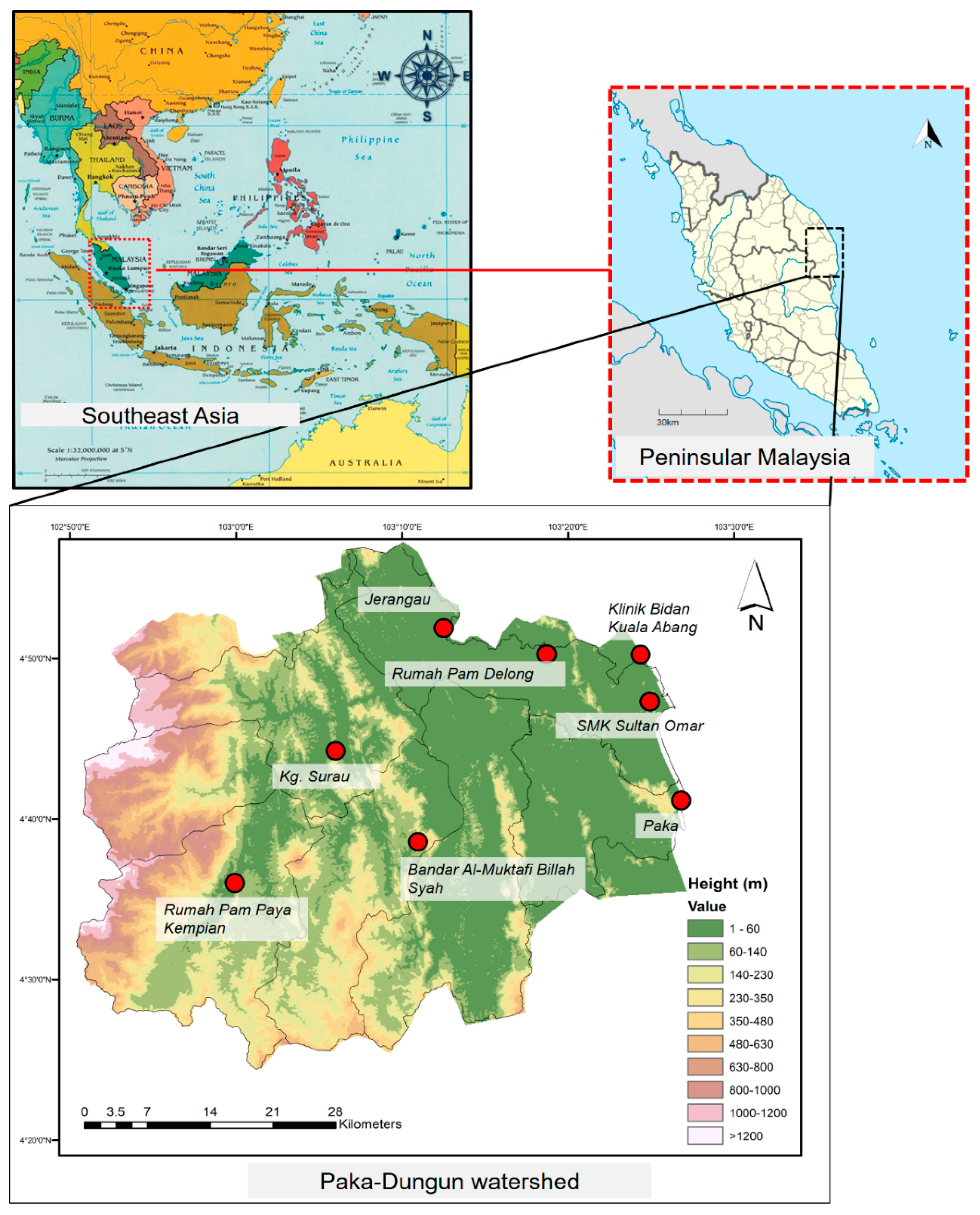
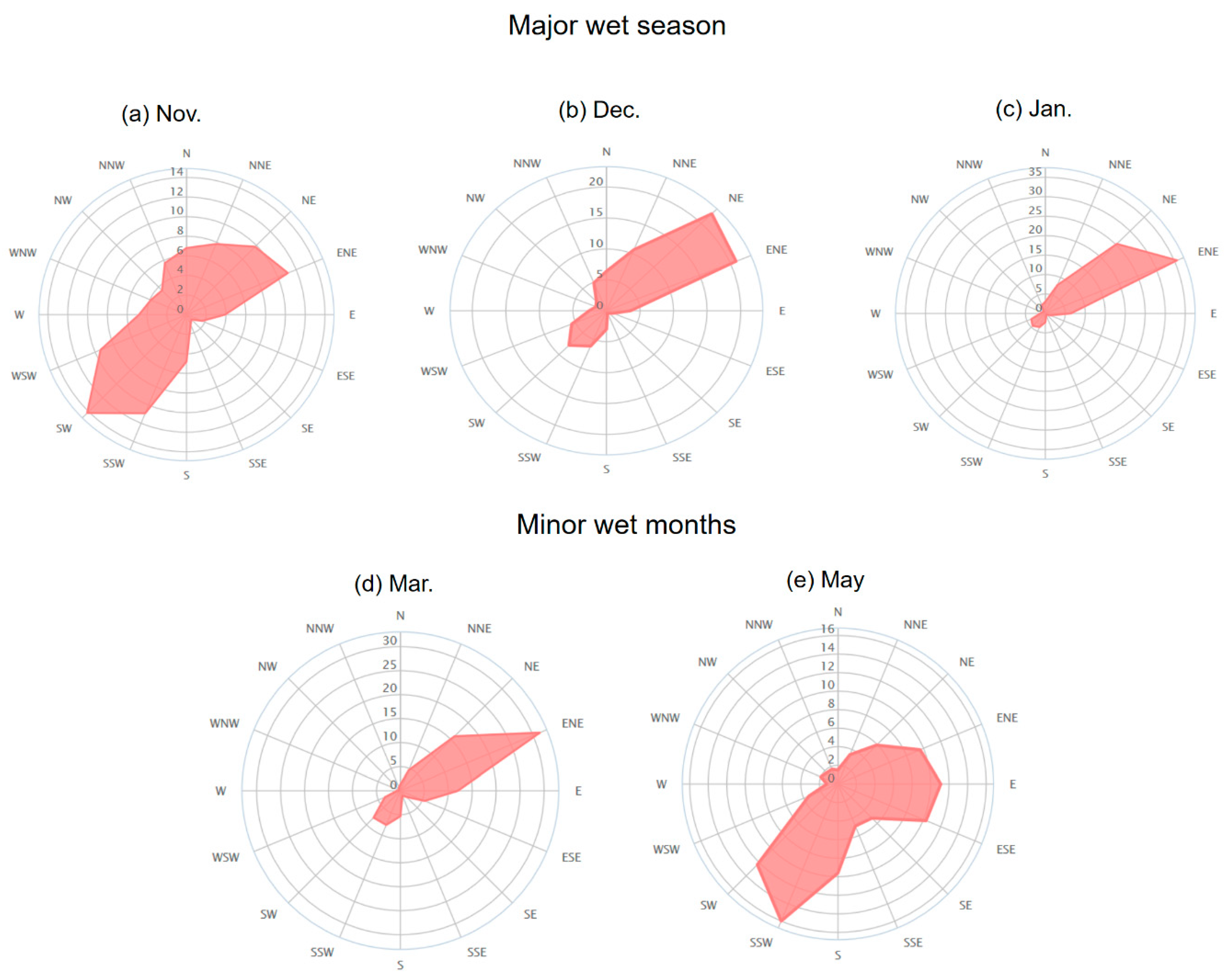
Paka-Dungun watershed is located in Peninsular Malaysia (4.75° N, 103.25° E), in the centre of Southeast Asia (Figure 1). This tropical coastal watershed has a total catchment area of 2430 square kilometres (243,000 ha). This watershed faces the South China Sea. The upper watershed comprises the hilly mountain of Gunung Chemerong (~1100 m). It has a humid tropical climate with a temperature range from 25 to 34°C and a total average annual rainfall of 3172 mm. Of the total rainfall, 39% (1100 mm) is received during the northeast monsoon season (November–January). This heavy rainfall is associated with a large volume of moisture coming from the South China Sea in the northeast direction (Figure 2a–c) and interaction with the orographic influences of the hilly areas (refer to the 2D view of the digital elevation model in Figure 1).
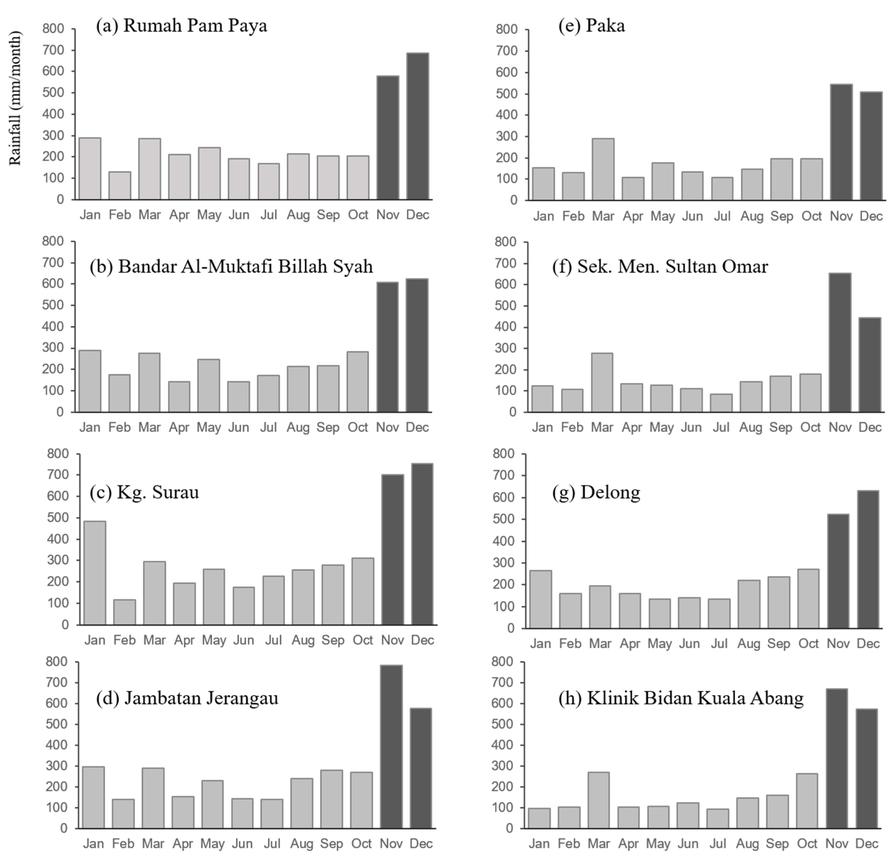
There is no distinct dry season, where the average rainfall for the rest of the month is 150 mm (refer hyetograph in Figure 3a–h). In some parts of the watershed, slight heavier rainfall in March and May, particularly due to the shifting from Northeast to Southwest monsoon. There are seven major sub-watersheds. Those sub-watersheds are the catchments for two major rivers, Sungai Paka (18 km length) and Sungai Dungun (33 km length). The major land cover is tropical forest (51%), followed by oil palm (31%), built up areas (10%), and others (9%), which includes mixed horticulture, orchard, aquaculture and other economic activities. One dam (Paka dam) is in this watershed for water resources supply. This watershed has constantly experienced flooding due to extreme river discharge and high tides, particularly during the wet season in November to January.
The digital elevation model (DEM) data, which are used to provide the topographic information and to represent the orographic factors of the watershed, is a product from the Shuttle Radar Topography Mission (SRTM). The DEM data product provides elevation information at 1 arc resolution (~30 m) and can be accessed at dwtkns.com/srtm30m/. For this study, the DEM has been re-gridded to 0.02° resolution. The elevation is based on EGM96 vertical datum. The elevation for the study area was extracted from the downloaded dataset using the catchment boundary information and is done by the ArcGIS software.
2.2. Precipitation and Wind Data
2.2.1. Global Precipitation Mission (GPM) Satellite Data
We used the hourly rainfall estimates data from the GPM satellite as our primary data. We utilized the multi-satellite precipitation estimate with climatological gauge calibration—Late Run, or also known as GPM_3IMERGHHL v06. This data product provides the half-hourly rain rate values. The main reasons for its selection are: (i) satellite rainfall estimates with finest gridded data (0.1°), (ii) high temporal data supply, ranging from half-hourly to daily and monthly. The public domain data ae obtained via the world wide web. GPM satellite precipitation is the successor of the Tropical Rainfall Measuring Mission (TRMM), and only available starting from April 2014. The downloaded data were then cropped for the selected catchment of our study area. We only chose the hourly data with an intensity of over 0.05 mm/half hour. Data with an average rainfall below that threshold were considered as no rain. The sampling period was conducted over the 24 h period starting from 8.00 am on the starting day until 8.00 am on the next day.
To assist our successful selection of the satellite data, we used the existing rain gauge records to filter the significant rainy days which have moderate to heavy intensity (daily rainfall exceeding 10 mm/d). The selection of the threshold was set so because, in theory, low-intensity rainy days tend to have an insignificant impact on the run-off or productivity of the catchment. From the sampling period, the datasets would be split into two, one is for the normal season (June–July) and second is the wet season (October–December) in 2014. From the 153 days of the sampling period, we had identified 46 significant rainy days to be used as samples, (daily rainfall exceeding 10 mm/d). The heaviest daily rainfall was 295 mm, indicated in Kg Surau station. The rest of the rainy days below 10 mm/d were excluded in our experiment.
2.2.2. Rain Gauge Data
There were eight rain gauges obtained from the Dept. of Irrigation and Drainage, Malaysia, used in this study. The locations of the stations, average elevation, and maximum elevation of their surrounding areas are included in Table 1. These stations were selected due to their preferences to represent the fair distribution of rainfall variation and various elevations in the study area. The rain gauge data were used for accuracy evaluation. The location of each station is shown in Figure 1.
2.2.3. Wind Data
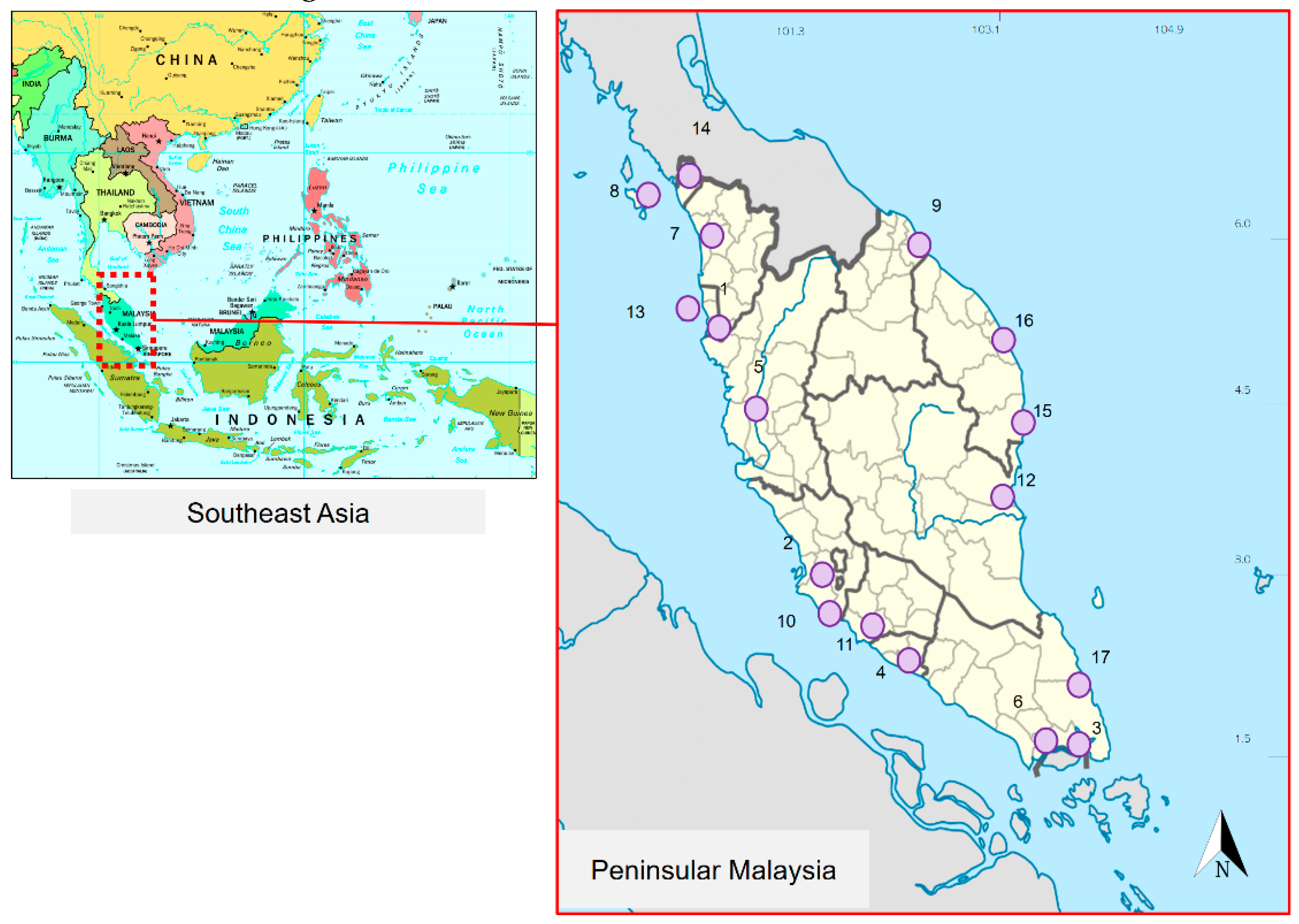
The hourly wind speed and its direction were obtained from the spline-interpolated products from the regional stations. The resolution is set to be similar to the desired downscaled resolution (0.02°). All of the data were acquired from the meteorological stations available at the local airports and also the Malaysian Meteorological Department. The geographic locations of the data were provided in Table 2 and Figure 4.
2.3. Downscaling Approach
The core principle of the downscaling process is to compute the ground rainfall based on the three factors, precipitation efficiency, condensation rate, and synoptic rain rate estimates at the exact hour of the rainfall occurrence. The exact timing and synoptic rain rate estimates of rainfall occurrence were provided by hourly data analysis of the GPM satellite data. In this study, only GPM data that have over 0.1 mm of rain per hour were considered for downscaling. Therefore, a preliminary selection of hourly rain rate images will be conducted before proceeding to the further downscaling process.
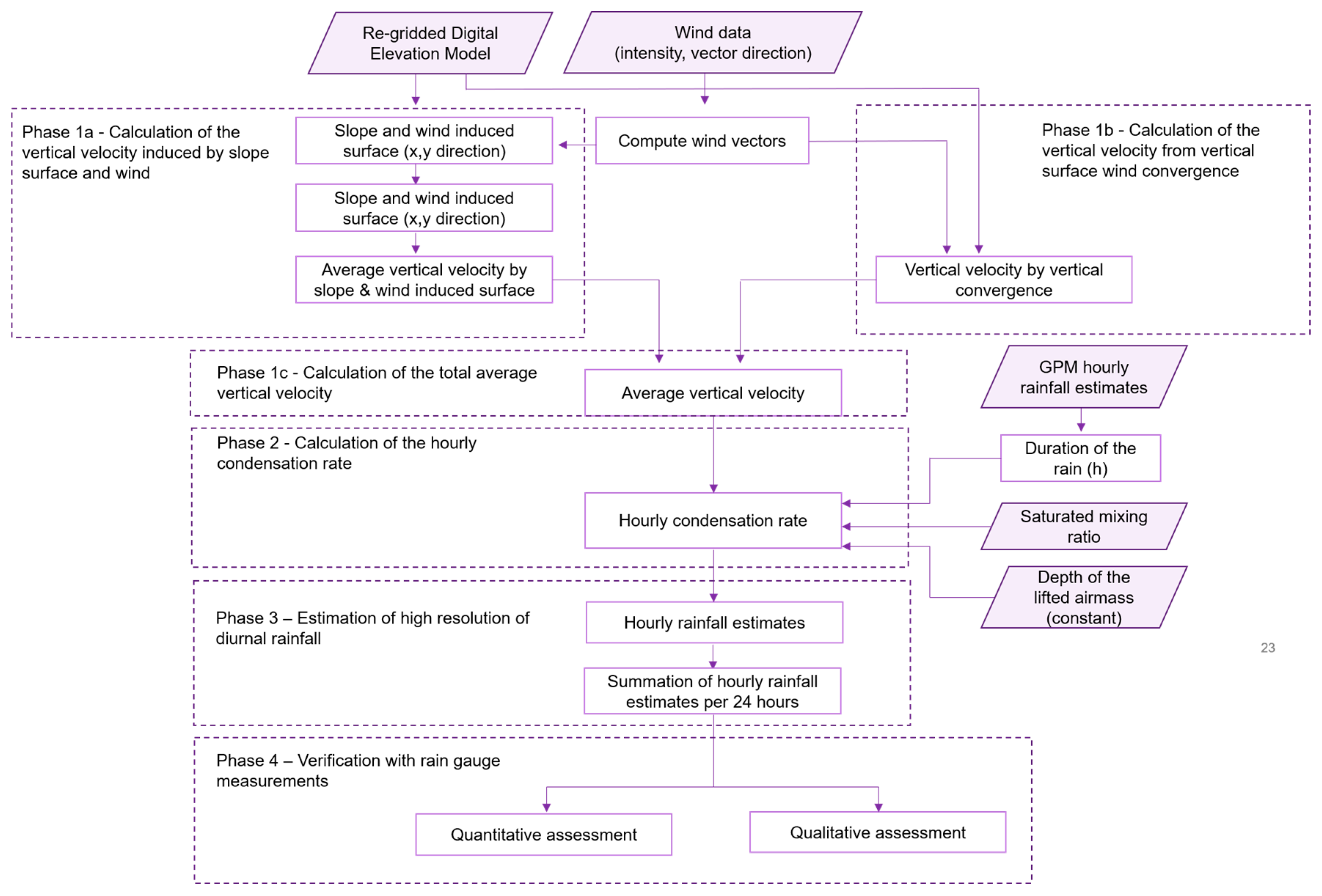
Because the satellite rainfall retrieval algorithm is based on the microwave backscatter from the cloud, the estimated rain rate is less sensitive to the orographic effects, which strongly influenced those watersheds that are mountainous and experience strong wind flows from the open sea. We adopted the theory that coupling the high resolution orographic and wind effect with coarse GPM rain rate data would represent the actual amount of the precipitation that reaches the ground, thus producing rainfall surface images with finer resolution that are suitable for the micro-watershed application. The methodology of this study is divided into four main phases, (1) computation of the total vertical velocity, (2) computation of the hourly condensation, (3) estimation of the high-resolution daily rainfall and (4) accuracy assessment. Figure 5 showed the schematic flow of the methodology.
2.3.1. Phase 1a—Calculation of the Vertical Velocity Induced by Slope Surface and Wind
The vertical velocity, which is the main component in this downscaling scheme, is computed in three major steps, (i) component A—calculation of the vertical velocity induced by slope surface and wind, (ii) component B—calculation of the vertical velocity from vertical convergence, and (iii) calculation of the total average vertical velocity. An orographic model introduced by Mass–Dempsey [27] was modified to suit the nature of the uniform gridded remote sensing data. This model was chosen due to several reasons, (1) they applied the concept of coupling the synoptic rain rate with the local orography in estimating local rainfall at near coast watershed; a concept that is suitable to be used in downscaling the satellite precipitation in Southeast Asia as many critical watersheds are in close proximity to the sea, (2) the sigma coordinate model adopted in the original version suits the nature of the uniform gridded data, (3) the simplicity of the calculation and number of required input parameters; because the calculation using new generation of remote sensing data dealt with huge gridded data, it would fasten the calculation process. In addition, the experimental site fulfils the fundamental requirement of the model that depends on vertical stability, hydrostatic assumptions and drive with strong exert of adiabatic convective process. With minimum field data being required (only wind data are regularly required), the downscaling process would be operational.
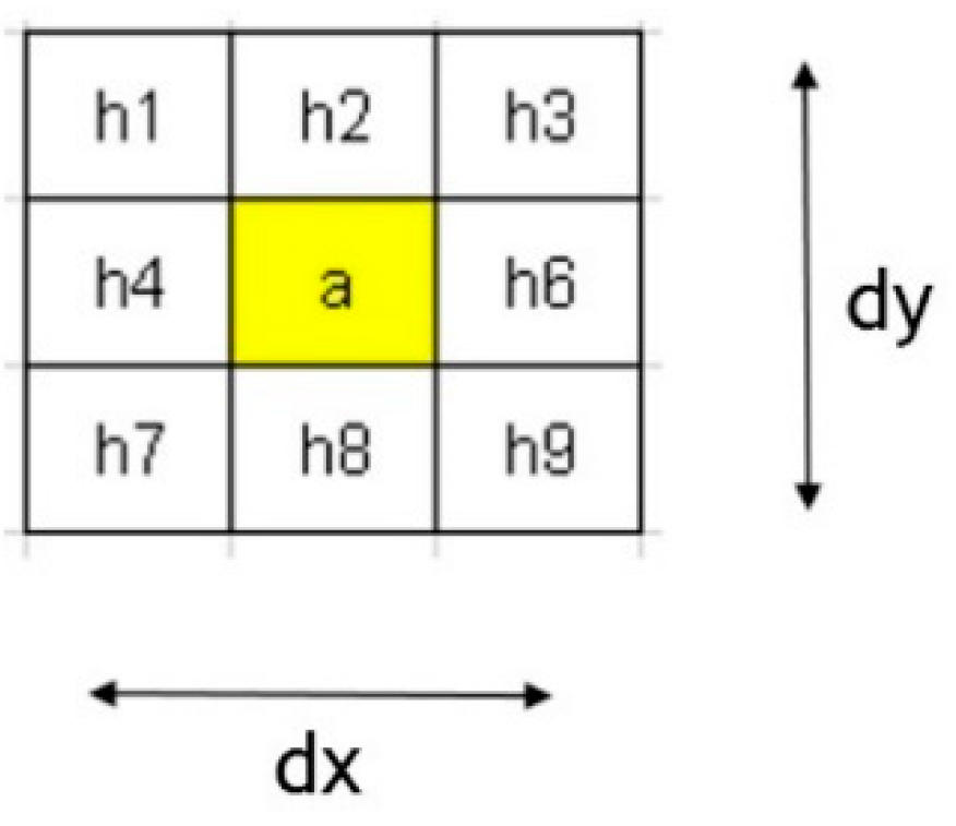
The first component is calculated based on the product of wind intensity vectors and slope parallel surface wind field, as shown in Equations (1)–(4). Instead of using four adjacent grid heights in the traditional Mass–Dempsey sigma coordinates model, we adapted eight adjacent heights in order to suit the nature of 3 × 3 kernel to the continuous DEM data.
where dh/dx and dh/dy are the slope induced surface in direction-x (east–west) and direction-y (north–south), respectively, h is the height from the DEM of surrounding central pixel (refer to Figure 6).
The wind vector effect was then incorporated with this slope-induced surface to transform the equation into
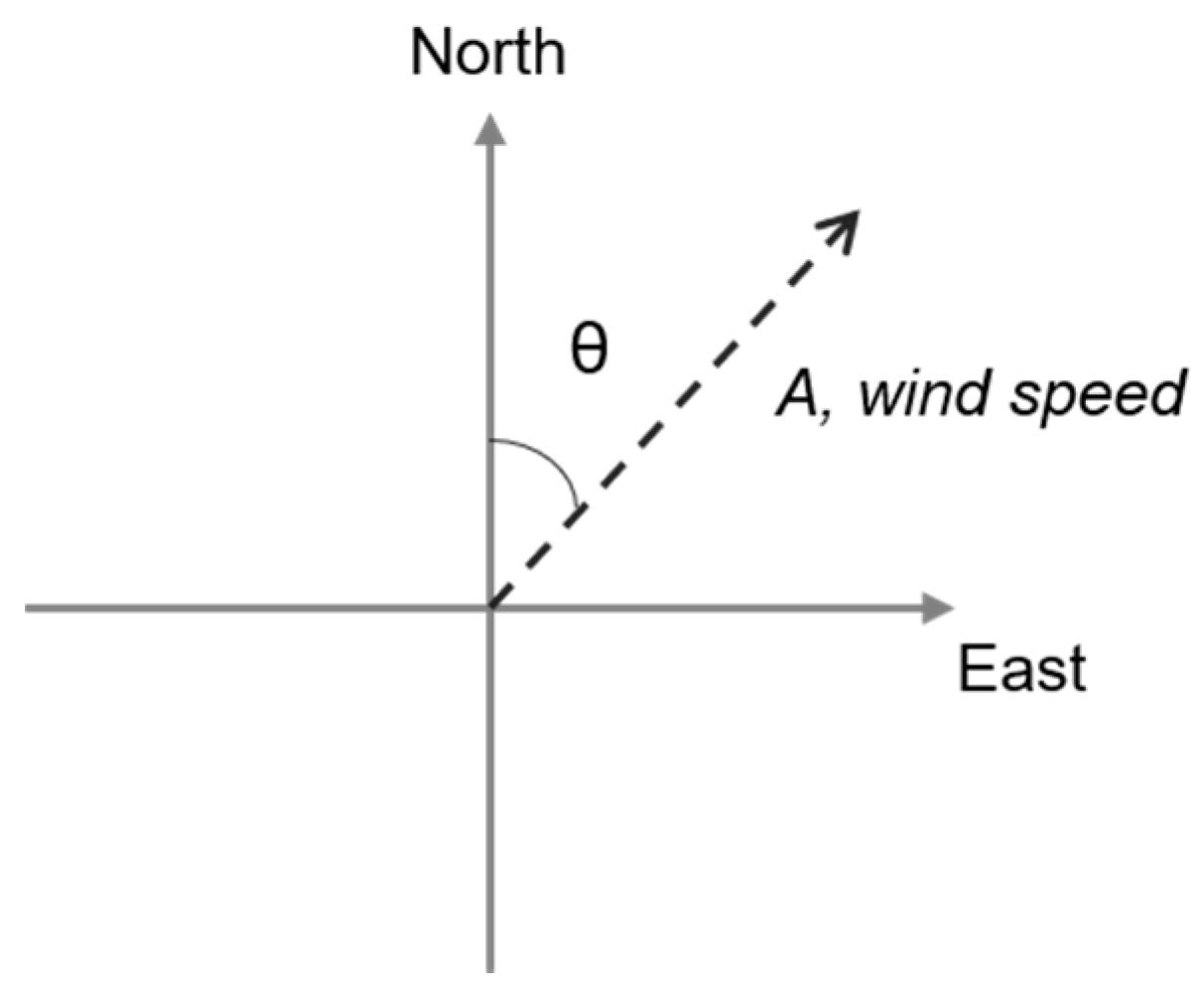
where ws is the total vertical velocity induced by slope surface and wind, wsx and wsy is the vertical velocity induced by slope surface and wind in the east–west and north–south directions, respectively, dx and dy is the distance between the east–west and north–south pixels, respectively, u and v are the wind vectors in the direction of east–west and north–south, respectively, a is the wind speed (km/h, later this metric unit is converted into m/h), and θ is the wind direction. See Figure 7 for the schematic diagram.
This vertical velocity induced by slope and wind surface will be computed for each hourly datum during the entire rainy period.
2.3.2. Phase 1b—Calculation of the Vertical Velocity from Vertical Surface Wind Convergence
The vertical velocity from vertical surface wind convergence is computed by summing the wind vectors (east–west and north–south direction) for each individual pixel. The assumption of the original Mass–Dempsey wind model where the surface wind convergences to decrease linearly with increasing height and becomes zero at a maximum of 2000 m, suitable with the elevation range of our study area (max. height ~ 1600 m). Therefore, the model can resemble effective vertical surface wind convergence at ground scale.
Theoretically, the wind speed intensity in this study is based on the synoptic scale and having a constant value with height. This is due to eliminating the effects of surface wind flow.
where dwc/dz is the vertical velocity at surface convergence, and du/dx and dv/dx are the wind vector components.
2.3.3. Phase 1c—Calculation of the Total Average Vertical Velocity
In order to obtain the total vertical velocity component, we average both the vertical velocity that acquired earlier in phase 1a and 1b.
2.3.4. Phase 2—Calculation of the Hourly Condensation Rate
Upon the derivation of vertical velocity, it is used then to compute the condensation, which represents the conversion of the airmass to liquid. We fully adopt the initial calculation by Mass–Dempsey, as shown in Equation (9). In short, condensation is obtained by the function of vertical velocity, rate of saturated mixing ratio, and depth of lifted airmass within the duration of the precipitation.
where Wt is the vertical velocity, dq/dz is the average saturated mixing ratio, D is a depth of the lifted airmass (height in m), and t is the duration (hour) of the precipitation. The value of the alternative value of dq/dz can be obtained from the pseudo-adiabatic chart. In this study, we refer to that option where the value of altitude is referred to the digital elevation model.
2.3.5. Phase 3—Estimation of High Resolution of Daily Rainfall
In this third phase, the daily rainfall for each high-resolution grid is computed in two steps. The first step is computing the downscale of hourly rainfall using the condensation information acquire in phase 2. The downscaled rainfall is equal to the product of condensation (C) and precipitation efficiency (E) added to the average synoptic precipitation over the ocean or flat terrain on adjacent land (Ps). In our study context, we substitute the Ps with the satellite rainfall estimates from GPM data, as expressed in Equation (10).
where Ph is the downscaled high-resolution rainfall at t hour, C is the condensation, E is the precipitation efficiency, and Ps is the satellite rainfall estimates from GPM. The precipitation efficiency for this area is assumed as a constant value of 0.8 based on the existing studies on many humid tropical sites [29,30]. i, and j represent the specific planimetric coordinates (x, y), and t is the specific duration of rainfall occurrences (in hour).
The second step is summing all the rainfall at t hours (Ph) in the 24 h period to obtain the total rainfall in a day. This process is executed at each high-resolution grid, and the final output of daily satellite rainfall is generated. Equation (11) describes the process.
where Pd is the total daily rainfall for each pixel in the i and j grid, and t is the total number of observations for each rainfall dataset.
2.3.6. Phase 4—Accuracy Assessment
We will evaluate the performance of the high-resolution downscaled rainfall quantitatively and qualitatively. The quantitative performance is measured by three indicators—the correlation, RMSE, and bias ration. Correlation is used to measure the strength of the relationship between the raw and downscale GPM rainfall against the rain gauge data over a series of temporal periods. Meanwhile, the RMSE, also referred to as the quantitative error, is used to measure the quantitative differences between downscaled rainfall and ground observed rainfall against the rain gauge. The third indicator, bias ratio, is used to quantify the proportion and trend of the deviation committed by the downscaled rainfall against the actual ground measurement. In this study, the bias ratio is used to assess how well the downscaled GPM data represent the rainfall pattern based on the ground rain gauge. A value of 1 indicates perfect representation of satellite and ground rainfall, while a value over 1 indicates satellite overestimation and below 1 means satellite underestimation. The calculation and concept of evaluation was adapted from Wolff et al. [31] and Mahmud et al. [13]. The corresponding equations are expressed below.
where Rs is the satellite-based rainfall, (raw and downscaled, depending on context), S is the standard deviation, and Rrg is the rain gauge data.
3. Results
This section is divided into four sub-sections, where each section represents a different element of spatio-temporal rainfall data performance, including (1) spatial rainfall pattern and distribution, (2) temporal rainfall data, (3) quantitative rainfall measurement, and (4) effective rainfall visualization at micro-watersheds scale.
3.1. Spatial Rainfall Pattern Representation Assessment
The bias ratio between the satellite rainfall and rain gauge data was used as an indicator to assess the goodness of fit of the rainfall spatial pattern (Table 3). The downscaled data better represented actual rainfall spatial patterns, compared with the raw GPM data. However, bias ratio reduction was slightly affected by elevation. In comparison with raw rainfall data, the average bias ratio at high-elevation stations was reduced from 61% to 26%, whereas bias ratio at low-elevation stations was reduced from 64% to 35%. Thus, downscaled rainfall data generally tended to underestimate actual rainfall.
Downscaled satellite rainfall data occasionally overestimated rain gauge during heavy rainfall months (October–December). However, such instances were exceptionally rare and occurred at only one station (Klinik Bidan Kuala Abang). This overestimation may have been due to the close proximity of this station to the sea; raw GPM rainfall data pixels may have been mistakenly identified as land, instead of sea.
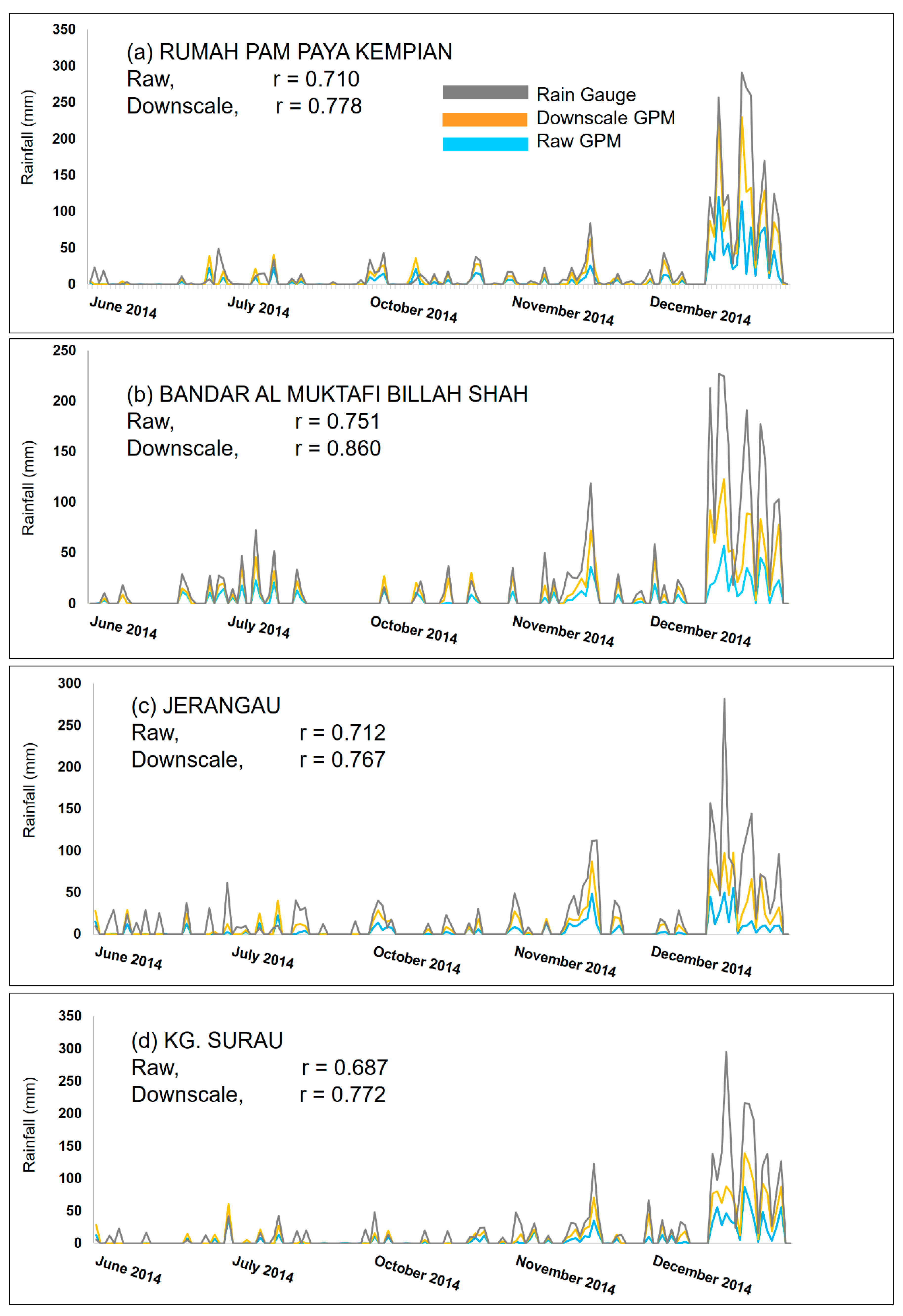
3.2. Temporal Rainfall Representation Assessment
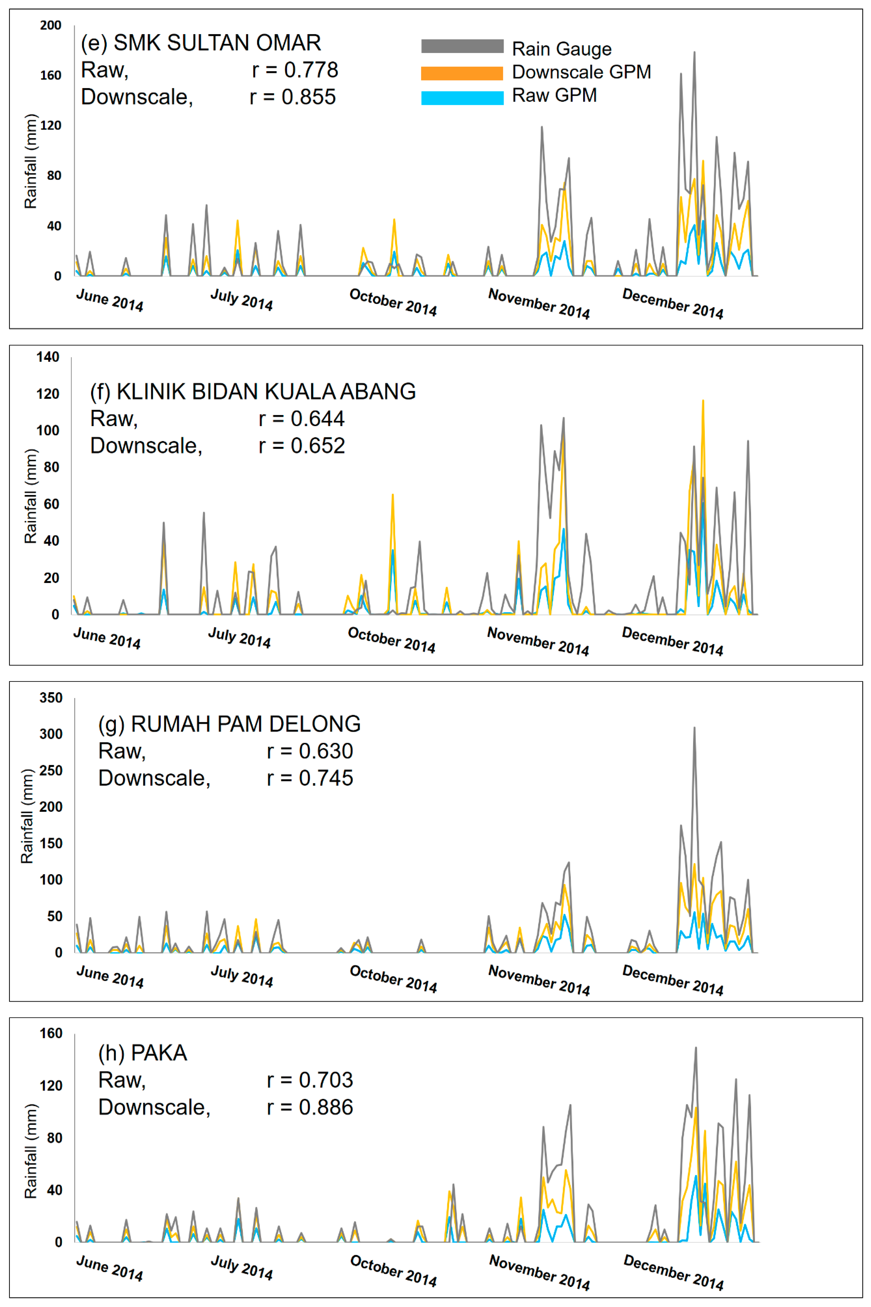
Time-series analyses showed an improvement in seasonal trends of downscaled GPM rainfall (Figure 8), with an increase in the correlation value from 18% to 22%. Greater bias was observed during the wet season, when downscaled GPM rainfall data consistently underestimated actual rainfall. Correlation was stronger at wetter stations (mainly at higher elevations) than at other stations; however, it was generally slightly lower (5%–8%) during the wet season, presumably due to greater error propagation during high-intensity rainfall.
3.3. Quantitative Rainfall Error Assessment
On average, downscaled GPM rainfall estimates showed smaller error values than the raw GPM rainfall estimates, with some variation among seasons and stations (Table 3). The quantitative accuracy of the downscaled rainfall estimates was better in the wet season than in the normal season; respective improvements of 34% and 25% were observed during November and December, compared with May and June. During the wet season, the error decreased from 41 to 27 mm/d, while the error during the normal season decreased from 16 to 12 mm/d. Error reduction capacity was higher at high-elevation stations (Rumah Pam Paya, Bandar Al-Muktafi Billah Shah and Kg. Surau), especially during the wet season.
The accuracy of downscaled rainfall data improved at high- and low-elevation stations (<80 m) by averages of 36% and 29%, respectively, in the wet season; these trends were not observed in the dry season. Greater error reduction was observed in the wet season than in the dry season. The downscaled GPM data always performed similarly to or better than the raw GPM data. No case where the downscaled GPM data performed worse than the raw GPM data was found.
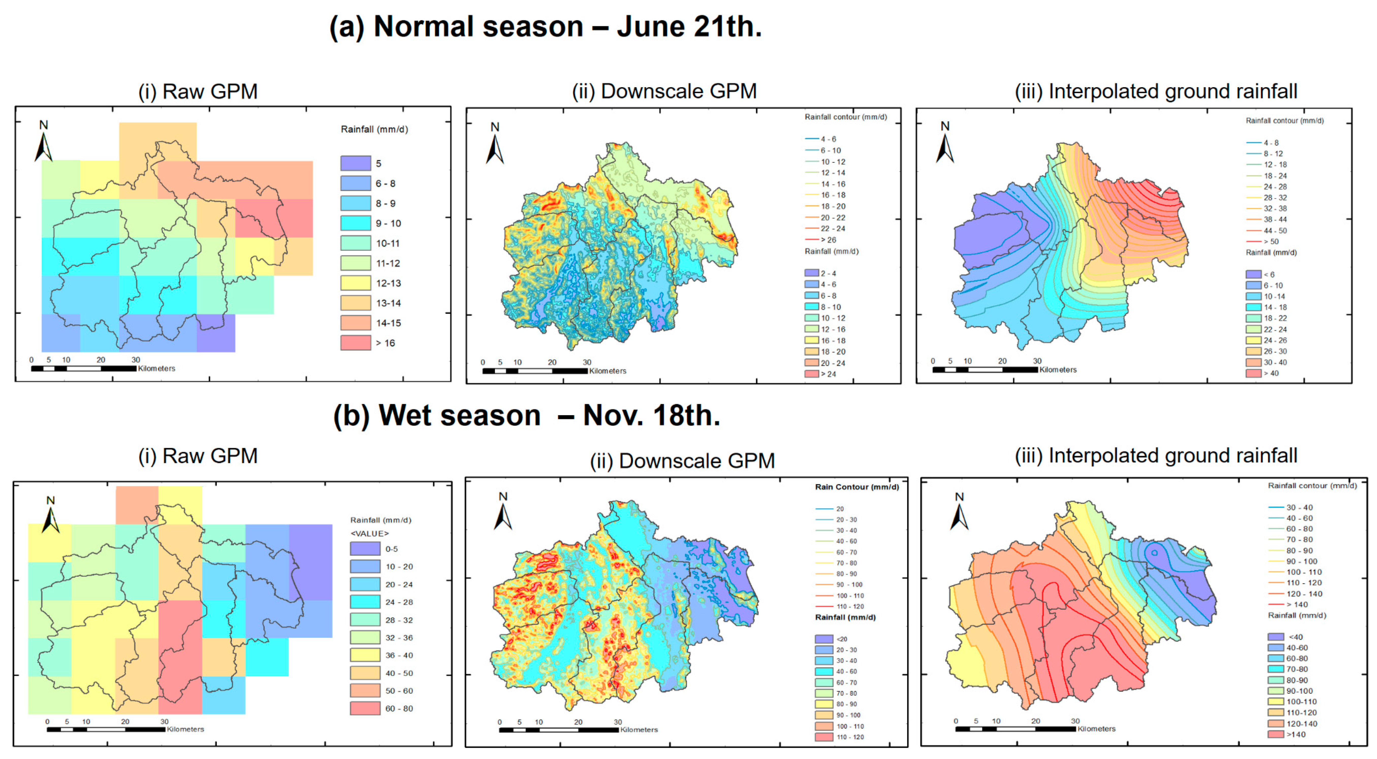
3.4. Qualitative Rainfall Assessment
Downscaled GPM rainfall data portrayed better rainfall variation than the raw GPM data during both seasons (Figure 9). Significant impact appeared at high elevated areas. The heavy rainfall in the high elevated areas that is caused by the interaction between the incoming atmospheric moisture from the northeast direction during the wet season is clearly depicted by the downscaled rainfall map. Hence, the downscaled GPM rainfall maps were also capable of depicting the likely pattern of the interpolated ground rainfall, with better localized rainfall pattern detail on the micro-catchments level.
4. Discussion
The proposed downscaling procedures were able to produce high-resolution daily rainfall data from GPM data. The downscaled rainfall data also had higher accuracy and qualitative ability compared to the raw GPM data. Without the use of rain gauge data, this downscaling technique is suitable for the data conflicting micro-watersheds. The outcome of the downscaling is also robust throughout any season despite relying on the regional wind data and elevation data as inputs. Hence, the downscaling technique is suitable for operational rainfall mapping, monitoring, and assessment. Although the ground precipitation radar can supply rainfall rate data with a fine spatiotemporal resolution, it is hindered by several limitations. Such limitations are poor data management and archiving, usage is limited for weather forecasting and difficult image data processing.
The downscaling technique could contribute to water resource management in the critical tropical micro-watersheds. Many water resources related micro-watersheds in Southeast Asia are highly vulnerable to drought and yet they suffer from a lack of rainfall data [32,33,34]. In addition, such watersheds also have a high risk of flooding and other related disasters (e.g., landslide) due to heavy and extreme rainfall. Therefore, the innovative solution of high-resolution daily rainfall maps would fill a significant gap on rainfall data in the effective water management and disaster framework [35].
There was a drawback that will need to be adhered to in the future works for the betterment of the algorithm. The first is regarding the slight underperformance at an elevation below 80 m. Because the downscaling algorithm incorporates an orography effect that strongly affects the undulated and higher elevation areas, the less elevated coastal areas could be strongly affected by other significant factors such as distance to the sea. A study by Hayward and Clarke [36] clarified the relationship between the rainfall and distance to the sea in Sierra Leone. Yamanaka [37] also highlighted this in his work on the equatorial coastal rainfall. Furthermore, the heat contrast differences between the land surface and sea temperature could play a role in influencing the rainfall distribution in tropical coastal areas [38,39]. More recent research highlighted the influence of coastline geomorphology on the rainfall distribution. This was indicated by Alfahmi et al. [40] and Yamanaka [41] in their work in Indonesia. Incorporating such variables into the downscaling procedures could be able to improve the output performance in the future.
The second limitation in our study is the use of interpolated regional wind data to represent the high-resolution of vertical velocity and condensation rate (0.02°). Since, in theory, vertical convection could happen at smaller region scales than 0.02°, our downscaling approach is therefore unable to represent such variation, and this might affect the accuracy of the results. Considering that capturing such high-resolution local wind data is a mounting challenge especially for a remote, forested, and mountainous watershed; the other plausible way to anticipate such limitation is through the innovation of various wind data downscaling methods, such as those introduced by Hasager [42] and Bentamy et al. [43]. However, obtaining both high-temporal and high-resolution (<0.25°) data is yet to be achieved. Nevertheless, with the accuracy that is obtained through the use of regional wind data, we believe that it was a worthwhile solution that could compromise the absolute absence of ground rain gauge data for many tropical micro-watersheds. A continuous improvisation is highly recommended and subjected to further research.
5. Conclusions
This study demonstrated that generating high-resolution daily rainfall from GPM satellite data can be materialized through the incorporation of high resolution orographic and vertical velocity factors obtained from regional wind data and the fine scale of a digital elevation model. The downscaled rainfall was able to produce a high-resolution rainfall with improved quantitative accuracy during both the wet and normal season, where the error is reduced by 34% and 16%, respectively. In addition, the spatial rainfall pattern and distribution is also increased by an average of 35%. Prior to this, the present spatial rainfall pattern accuracy for wet season had reached 75%, while being at 70% during the normal season. The visual appearances and quality of the downscaled rainfall maps were also improved significantly. The proposed downscaling algorithm can be useful in providing alternative rainfall data especially for the ungauged or data conflicting tropical micro-watersheds in coastal region. It was found that the sensitivity of the proposed algorithm was higher in the high elevated watershed region (>80 m a.s.l) during the wet season, where the strong monsoon wind and moist air masses characterize the local rainfall. The downscaling process on the watershed areas with low elevation (<80 m a.s.l) and located t near the coastal lines are suggested to incorporate additional downscaling factors such as distance to the sea, coastal line geomorphology and sea–land heat differences.
Author Contributions
Conceptualization, formal analysis, data curation, M.R.M. and A.A.M.Y.; Writing-review and editing, M.R.M., Project administration, funding acquisition, resources, M.H. and M.N.M.R. Supervision, M.R.M. and M.N.M.R. All authors have read and agreed to the published version of the manuscript.
Funding
This work was supported by Universiti Teknologi Malaysia through the Research University Grant (Q.J130000.2652.17J09) and High Impact Research (Q.J130000.2409.04G44) initiatives to encourage critical application research for tropical environment.
Acknowledgments
We would like to express our deepest gratitude to the data contributors namely Dept. of Irrigation & Drainage, Malaysia, National Aeronautics & Space Administration (NASA) Center for & Malaysian Meteorological Department. Also, we would like to thank all laboratory members and individuals who had contributed to the preparation of this manuscript.
Conflicts of Interest
The authors declare that the research has no conflict of interest.
References
- Vegas-Vilarrubia, T.; Maass, M.; Rull, V.; Elias, V.; Ramon, A.; Ovalle, C.; Lopez, D.; Schneider, G.; Depetris, J.; Douglas, I. Small catchment studies in the tropical zone. In Biogeochemistry of Small Catchments: A Tool for Environmental Research; Moldan, B., Cerny, J., Eds.; John Wiley & Sons, Ltd.: Hoboken, NJ, USA, 1994. [Google Scholar]
- IUWASH. Water Supply Vulnerability Assessment and Adaptation Plan; PDAM Pematangsiantar Summary Report; Indonesia Urban Water Sanitation and Hygience Project (IUWASH): Jakarta, Indonesia, August 2014; Available online: https://www.iuwashplus.or.id/cms/wp-content/uploads/2017/04/VAAP-Summary-Report-PDAM-Pematangsiantar.pdf (accessed on 13 November 2019).
- Toriman, M.E.; Abdullah, M.P.; Mokhtar, M.; Gasim, M.B.; Karim, O. Surface erosion and sediment yields assessment from small ungauged catchment of Sungai Anak Bangi Selangor. Malays. J. Anal. Sci. 2010, 14, 12–23. [Google Scholar]
- Bidin, K.; Chappell, N.A. First evidence of a structured and dynamic spatial pattern of rainfall within a small humid tropical catchment. Hydrol. Earth Syst. Sci. 2003, 7, 245–253. [Google Scholar] [CrossRef] [Green Version]
- Su, Y.; Zhao, C.; Wang, Y.; Ma, Z. Spatiotemporal Variations of Precipitation in China Using Surface Gauge Observations from 1961 to 2016. Atmosphere 2020, 11, 303. [Google Scholar] [CrossRef] [Green Version]
- Kim, I.-W.; Oh, J.; Woo, S.; Kripalani, R.H. Evaluation of precipitation extremes over the Asian domain: Observation and modelling studies. Clim. Dyn. 2019, 52, 1317–1342. [Google Scholar] [CrossRef] [Green Version]
- Cheong, W.K.; Timbal, B.; Golding, N.; Sirabaha, S.; Kwan, K.F.; Cinco, T.A.; Archevarahuprok, B.; Vo, V.H.; Gunawan, D.; Han, S. Observed and modelled temperature and precipitation extremes over Southeast Asia from 1972 to 2010. Int. J. Clim. 2018, 38, 3013–3027. [Google Scholar] [CrossRef]
- Mahmud, M.R.; Hashim, M.; Matsuyama, H.; Numata, S.; Hosaka, T. Spatial Downscaling of Satellite Precipitation Data in Humid Tropics Using a Site-Specific Seasonal Coefficient. Water 2018, 10, 409. [Google Scholar] [CrossRef] [Green Version]
- Behrangi, A.; Khakbaz, B.; Jaw, T.C.; AghaKouchak, A.; Hsu, K.; Sorooshian, S. Hydrologic evaluation of satellite precipitation products over a mid-size basin. J. Hydrol. 2011, 360, 225–237. [Google Scholar] [CrossRef] [Green Version]
- Zhang, Y.; Li, Y.; Ji, X.; Luo, X.; Li, X. Fine-Resolution Precipitation Mapping in a Mountainous Watershed: Geostatistical Downscaling of TRMM Products Based on Environmental Variables. Remote Sens. 2018, 10, 119. [Google Scholar] [CrossRef] [Green Version]
- Mahmud, M.R.; Numata, S.; Hosaka, T.; Matsuyama, H.; Hashim, M. Preliminary study for effective seasonal downscaling of TRMM precipitation data in Peninsular Malaysia: Local scale validation using high resolution areal precipitation. Remote Sens. 2015, 7, 4092–4111. [Google Scholar] [CrossRef] [Green Version]
- Hou, A.Y.; Kakar, R.K.; Neeck, S.; Azarbarzin, A.A.; Kummerow, C.; Kojima, M.; Oki, R.; Nakamura, K.; Iguchi, T. The global precipitation measurement mission. Bull. Amer. Meteor. Soc. 2014, 95, 701–722. [Google Scholar] [CrossRef]
- Mahmud, M.R.; Hashim, M.; Reba, M.N.M. How effective is the new generation of GPM satellite precipitation in characterizing the rainfall variability over Malaysia? Asia-Pac. J. Atmos. Sci. 2017, 53, 375. [Google Scholar] [CrossRef]
- Duan, Z.; Bastiaanssen, W.G.M. First results from Version 7 TRMM 3B43 precipitation product in combination with a new downscaling-calibration procedure. Remote Sens. Environ. 2013, 131, 1–13. [Google Scholar] [CrossRef]
- Chen, F.; Liu, Y.; Liu, Q.; Li, X. Spatial downscaling of TRMM 3B43 precipitation considering spatial heterogeneity. Int. J. Remote Sens. 2014, 35, 3074–3093. [Google Scholar] [CrossRef]
- Ulloa, J.; Ballari, D.; Campozano, L.; Samaniego, E. Two-step downscaling of TRMM 3B43 V7 precipitation in contrasting climatic regions with sparse monitoring: The case of Ecuador in tropical South America. Remote Sens. 2017, 9, 758. [Google Scholar] [CrossRef] [Green Version]
- Shi, Y.; Song, L. Spatial Downscaling of Monthly TRMM Precipitation Based on EVI and Other Geospatial Variables Over the Tibetan Plateau From 2001 to 2012. Mt. Res. Dev. 2015, 35, 180–194. [Google Scholar] [CrossRef]
- Hunink, J.E.; Immerzeel, W.W.; Droogers, P. A high-resolution precipitation 2-step mapping procedure (HiP2P): Development and application to a tropical mountainous area. Remote Sens. Environ. 2014, 140, 179–188. [Google Scholar] [CrossRef]
- Sharifi, E.; Saghafian, B.; Steinacker, R. Downscaling satellite precipitation estimates with multiple linear regression, artificial neural networks, & spline interpolation techniques. J. Geo. Res. Atmos. 2019, 124, 780–805. [Google Scholar]
- Park, N.-W. Spatial downscaling of TRMM precipitation using geostatistics and fine scale environmental variables. Adv. Meteorol. 2013, 2013, 237126. [Google Scholar] [CrossRef]
- Ceccherini, G.; Ameztoy, I.; Hernández, C.P.R.; Moreno, C.C. High-resolution precipitation datasets in South America and West Africa based on satellite-derived rainfall, enhanced vegetation index and digital elevation model. Remote Sens. 2015, 7, 6454–6488. [Google Scholar] [CrossRef] [Green Version]
- Ryo, M.; Valeriano, O.C.S.; Kanae, S.; Ngoc, T.D. Temporal downscaling of daily gauged precipitation by application of a satellite producto for flood simulation in a poorly gauged basin & its evaluation with multiple regression analysis. J. Hydrometeorol. 2014, 15, 563–580. [Google Scholar]
- Chen, F.; Gao, Y.; Wang, Y.; Qin, F.; Li, X. Downscaling satellite-derived daily precipitation products with an integrated framework. Int. J. Climatol. 2018, 39, 1287–1304. [Google Scholar] [CrossRef]
- Lopez, P.L.; Immerzeel, W.W.; Sandoval, E.A.R.; Sterk, G.; Schellekens, J. Spatial downscaling of satellite-based precipitation and its impact on discharge simulations in the Magdalena River basin in Colombia. Front. Earth Sci. 2018, 6. [Google Scholar] [CrossRef] [Green Version]
- Bachok, M.F.; Shamsudin, S.; Abidin, R.A.; Jeevaragagam, P.; Harun, S. Assessment of observational data in Peninsular Malaysia for verification of windstrom-prroducing thunderstorms nowcast systems. Int. J. Appl. Environ. Sci. 2017, 12, 2107–2122. [Google Scholar]
- Manzanas, R. Statistical downscaling in the tropics can be sensitive to reanalysis choice: A Case Study for Precipitation in the Philippines. J. Clim. 2015, 28, 4171–4184. [Google Scholar] [CrossRef]
- Gusain, A.; Vittal, H.; Kulkarni, S.; Ghosh, S.; Karmakar, S. Role of vertical velocity in improving finer scale statistical downscaling for projection of extreme precipitation. Theor. Appl. Clim. 2018, 137, 791–804. [Google Scholar] [CrossRef]
- Mass, C.F.; Dempsey, D.P. A One-Level, Mesoscale Model for Diagnosing Surface Winds in Mountainous and Coastal Regions. Mon. Weather. Rev. 1985, 113, 1211–1227. [Google Scholar] [CrossRef] [Green Version]
- Li, X.; Sui, C.H.; Lau, K.-M. Precipitation efficiency in the tropical deep convective region: A 2-D cloud resolving modeling study. J. Met. Japan 2002, 80, 205–212. [Google Scholar]
- Narsey, S.; Jakob, C.; Singh, M.S.; Bergemann, M.; Louf, V.; Protat, A.; Williams, C. Convective Precipitation Efficiency Observed in the Tropics. Geophys. Res. Lett. 2019, 46, 13574–13583. [Google Scholar] [CrossRef]
- Wolff, D.B.; Marks, D.A.; Amitai, E.; Silberstein, D.S.; Fisher, B.L.; Tokay, A.; Wang, J.; Pippitt, J.L. Ground Validation for the Tropical Rainfall Measuring Mission (TRMM). J. Atmospheric Ocean. Technol. 2005, 22, 365–380. [Google Scholar] [CrossRef]
- Trindade, L.D.L.; Scheibe, L.F. Water Management: Constraints to and Contributions of Brazilian Watershed Management Committees; Ambiente & Sociedade: Sao Paulo, Brazil, 2019; Volume 22. [Google Scholar]
- Miyan, M.A. Droughts in Asian Least Developed Countries: Vulnerability and sustainability. Weather. Clim. Extremes 2015, 7, 8–23. [Google Scholar] [CrossRef] [Green Version]
- United Nation. Ready for the Dry Years, Building Resilience to Drought in South-East Asia; United Nations Publication: Bangkok, Thailand, 2019. [Google Scholar]
- Gariano, S.F.; Guzzeti, F. Landslides in a changing climate. Earth-Sci. Rev. 2016, 162, 227–252. [Google Scholar] [CrossRef] [Green Version]
- Hayward, D.; Clarke, R.T. Relationship between rainfall, altitude and distance from the sea in the Freetown Peninsula, Sierra Leone. Hydrol. Sci. 1996, 41, 377–384. [Google Scholar] [CrossRef]
- Yamanaka, M.D. Climate-biogeosphere-humanosphere interaction. Conference: 1st Int. School on Equatorial Atmosphere (ISQUAR). In Proceedings of the 98th Symposium on Sustainable Humanosphere, Bandung, Indonesia, 18–22 March 2019; Available online: http://situs.opi.lipi.go.id/hss2019/ (accessed on 20 December 2019).
- Houze, R.A.; Geotis, S.G.; Marks, F.D.; West, A.K. Winter monsoon convection in the vicinity of North Borneo.Part I: Structure and time variation of the clouds and precipitation. Mon. Weather. Rev. 1981, 109, 1595–1614. [Google Scholar] [CrossRef] [Green Version]
- Wu, P.; Hara, M.; Hamada, J.; Yamanaka, M.D.; Kimura, F. Why a large amount of rain falls over the sea in the vicinityof western Sumatra Island during nighttime. J. Appl. Meteor. Climatol. 2009, 48, 1345–1361. [Google Scholar] [CrossRef]
- Alfahmi, F.; Boer, R.; Hidayat, R.; Perdinan Sopaheluwakan, A. The impact of of concave coastline on rainfall offshore distribution over Indonesian Maritime Continent. Sci. World J. 2019, 2019, 6839012. [Google Scholar] [CrossRef] [PubMed] [Green Version]
- Yamanaka, M.D. Physical climatology of Indonesian Maritime Continent: An outline to comprehend observational studies. Atmos. Res. 2016, in press. [Google Scholar] [CrossRef] [Green Version]
- Hasager, C.B. Offshore winds mapped from satellite remote sensing. WIREs Energy Environ. 2014, 3, 594–603. [Google Scholar] [CrossRef] [Green Version]
- Bentamy, A.; Denis, C.-F. Gridded surface wind fields from Metop/ASCAT measurements. Int. J. Remote Sens. 2012, 33, 1729–1754. [Google Scholar] [CrossRef] [Green Version]
Figure 1.
Study area. The red dots are the locations of the rain gauges.

Figure 2.
Rose wind vector during major wet season (a) November; (b) December; and (c) January and minor wet months (d) March; & (e) May.
Figure 2.
Rose wind vector during major wet season (a) November; (b) December; and (c) January and minor wet months (d) March; & (e) May.

Figure 3.
Hyetograph (1988–2016) for all the rain gauge stations of the study area.

Figure 4.
The geographic locations of the wind stations.

Figure 5.
Schematic flow of methodology.

Figure 6.
Kernel used to compute the vertical velocity.

Figure 7.
Kernel used to compute the vertical velocity 2b Schematic diagram for wind vector calculation.
Figure 7.
Kernel used to compute the vertical velocity 2b Schematic diagram for wind vector calculation.

Figure 8.
Time-series between the rain gauge, raw and downscaled Global Precipitation Mission (GPM) at rain gauge stations. Rain days below than 10 mm/day were considered as low rainfall days and excluded in the calculation.
Figure 8.
Time-series between the rain gauge, raw and downscaled Global Precipitation Mission (GPM) at rain gauge stations. Rain days below than 10 mm/day were considered as low rainfall days and excluded in the calculation.


Figure 9.
Samples of the raw and downscaled GPM rainfall maps and also the interpolated rainfall using the rain gauges. (a) Normal season; (b) wet season.
Figure 9.
Samples of the raw and downscaled GPM rainfall maps and also the interpolated rainfall using the rain gauges. (a) Normal season; (b) wet season.


Table 1.
Rain gauge details.
| Stations | Name | Locations | Elevation (m) | ||
|---|---|---|---|---|---|
| E | N | Average | Maximum (2 km Radius) | ||
| 4529001 | Rumah Pam Paya, Pasir Raja | 102.98 | 4.57 | 70 | 200 |
| 4631001 | Bandar Al-Muktafi Billah Shah | 103.19 | 4.62 | 60 | 170 |
| 4634085 | Pusat Kesihatan Paka | 103.44 | 4.64 | 11 | 12 |
| 4730002 | Kg. Surau | 103.09 | 4.74 | 38 | 210 |
| 4734079 | SMK Sultan Omar | 103.42 | 4.77 | 11 | 13 |
| 4834001 | Klinik Bidan Kuala Abang | 103.31 | 4.82 | 12 | 24 |
| 4833078 | Rumah Pam Delong | 103.42 | 4.83 | 22 | 23 |
| 4832011 | Jerangau | 103.20 | 4.85 | 20 | 80 |
Table 2.
Wind station details.
| No | Station Name | Lat. | Long. |
|---|---|---|---|
| 1 | Bayan Lepas | 5.30 | 100.48 |
| 2 | Subang | 3.15 | 101.70 |
| 3 | Pasir Gudang | 1.45 | 103.88 |
| 5 | Malacca | 2.20 | 102.25 |
| 6 | Ipoh | 4.62 | 101.12 |
| 7 | Johor Bahru | 1.47 | 103.77 |
| 8 | Alor Setar | 6.12 | 100.37 |
| 9 | Langkawi | 6.32 | 100.37 |
| 10 | Kota Bahru | 6.12 | 102.25 |
| 11 | KLIA | 2.82 | 101.80 |
| 12 | Seremban | 2.72 | 101.93 |
| 13 | Kuantan | 3.80 | 103.32 |
| 14 | Georgetown | 5.42 | 100.33 |
| 15 | Kangar | 6.43 | 100.20 |
| 16 | Cukai | 4.25 | 103.42 |
| 17 | Kuala Terengganu | 5.33 | 103.12 |
| 18 | Mersing | 2.43 | 103.83 |
Table 3.
Average quantitative error (RMSE) and bias ratio for all ground rain gauge before and after the downscaling process. * Bandar AMBS: Bandar Al-Muktafi Billah Shah.
Table 3.
Average quantitative error (RMSE) and bias ratio for all ground rain gauge before and after the downscaling process. * Bandar AMBS: Bandar Al-Muktafi Billah Shah.
| Stations No. | Name | Root Mean Square Error (mm/d) | Bias Ratio (Sat/Rg) | ||||||
|---|---|---|---|---|---|---|---|---|---|
| Wet Season (n = 21) | Normal Seaso(n = 18) | Wet Season (n = 21) | Normal Season (n = 18) | ||||||
| Raw | Downscale | Raw | Downscale | Raw | Downscale | Raw | Downscale | ||
| 4529001 | Rumah Pam Paya | 47 | 24 | 23 | 15 | 0.44 | 0.78 | 0.48 | 0.88 |
| 4631001 | *Bandar AMBS | 34 | 51 | 13 | 10 | 0.33 | 0.71 | 0.38 | 0.65 |
| 4832011 | Jerangau | 43 | 30 | 29 | 25 | 0.39 | 0.69 | 0.34 | 0.65 |
| 4730002 | Kg. Surau | 49 | 34 | 14 | 12 | 0.35 | 0.7 | 0.44 | 0.88 |
| 4734079 | SMK Sultan Omar | 34 | 24 | 12 | 10 | 0.33 | 0.71 | 0.31 | 0.71 |
| 4834001 | Klinik Bidan Kuala Abang | 26 | 23 | 11 | 9 | 0.62 | 1.12 | 0.3 | 0.61 |
| 4833078 | Rumah Pam Delong | 45 | 28 | 15 | 11 | 0.38 | 0.63 | 0.31 | 0.63 |
| 4634085 | Pusat Kesihatan Paka | 33 | 21 | 8 | 6 | 0.33 | 0.65 | 0.28 | 0.63 |
© 2020 by the authors. Licensee MDPI, Basel, Switzerland. This article is an open access article distributed under the terms and conditions of the Creative Commons Attribution (CC BY) license (http://creativecommons.org/licenses/by/4.0/).
Share and Cite
MDPI and ACS Style
Mahmud, M.R.; Mohd Yusof, A.A.; Mohd Reba, M.N.; Hashim, M. Mapping the Daily Rainfall over an Ungauged Tropical Micro-Watershed: A Downscaling Algorithm Using GPM Data. Water 2020, 12, 1661. https://doi.org/10.3390/w12061661
AMA Style
Mahmud MR, Mohd Yusof AA, Mohd Reba MN, Hashim M. Mapping the Daily Rainfall over an Ungauged Tropical Micro-Watershed: A Downscaling Algorithm Using GPM Data. Water. 2020; 12(6):1661. https://doi.org/10.3390/w12061661
Chicago/Turabian StyleMahmud, Mohd. Rizaludin, Aina Afifah Mohd Yusof, Mohd Nadzri Mohd Reba, and Mazlan Hashim. 2020. "Mapping the Daily Rainfall over an Ungauged Tropical Micro-Watershed: A Downscaling Algorithm Using GPM Data" Water 12, no. 6: 1661. https://doi.org/10.3390/w12061661
Note that from the first issue of 2016, this journal uses article numbers instead of page numbers. See further details here.