Second Order Glauber Correlation of Gravitational Waves Using the LIGO Observatories as Hanbury Brown and Twiss Detectors  ^†

Abstract

The second order Glauber correlation of a simplified gravitational wave is investigated, using parameters from the first signal detected by LIGO. This simplified model spans the inspiral, merger, and ringdown phases of a black hole merger and was created to have a continuous amplitude, so there is no discontinuity between the phases. This allows for a trivial extraction of the intensity, which is necessary for determining the correlation between detectors. The two LIGO observatories can be used as detectors in a Hanbury Brown and Twiss interferometer for gravitational waves; these observatories measure the amplitude of the wave, so these measurements were used as the basis of the simplified model. The signal detected by the observatories is transient and is not consistent with chaotic or steady electromagnetic waves and thus the second order Glauber correlation function was calculated to produce physically meaningful results. To find correlations that are consistent with applications to electromagnetic waves, weighting functions for both models were studied in the integral equations for the Glauber correlation functions. The relationship between the transient and chaotic signals of both waveforms and their respective correlation functions was also examined. The second order Glauber correlation functions are a measure of intensity interference between independent detectors and has proven to be useful in both optics and particle physics. It has also been used in theoretical studies of primordial gravitational waves. The correlations can be used to define the degrees of coherence of a field, characterize multi-particle processes and assist in image enhancement.

1. Introduction

The intention of this research is to develop techniques to find the 2nd order Glauber correlations of gravitational waves. Using the same methodology and characterizations used for electromagnetic waves has not been done with the intention of understanding and describing the fundamental structure of non-primordial gravitational waves. The analysis of a signal detected by LIGO introduces a problem; the signal received from a black hole merger is short lived, where meaningful detection is only observed for ∼0.2 s. This differs from signals analyzed by the quantum optics [1,2] and particle physics [3] communities, which are typically not transient. A method of calculating the second order Glauber correlation function utilizing intensity weighting is proposed; the method normally prescribed averages over a long time period, which does not yield a period-independent amplitude. Using the novel method, correlations are produced that are similar to already analyzed electromagnetic waves, and comparing the two can provide insight into gravitational waves.

2. Methods

Classically, interferometers are used to study the characteristics of waves by interfering the wave with itself. The LIGO observatories consist of two separate gravitational wave interferometers that measure the strain amplitude of the observed gravitational wave. Each of the two observatories can be thought of as the two detectors of an interferometer, allowing the intensity of the wave to be extracted and analyzed with the second order Glauber correlation function.

This function is a function of the time between detections that describes the correlations of observed intensities [1]. This calculation is defined as,

$$g^2\left(\tau \right)=\frac{\langle I\left(t\right)I(t+\tau )\rangle }{\langle I\left(t\right)\rangle \langle I(t+\tau )\rangle },$$

(1)

where $\tau$ is the time between detections. $\langle ...\rangle$ signifies a time averaging over a long time period [4]. Typically, the function is expanded using a standard time average of time T.

$$g^2\left(\tau \right)=\frac{\frac{1}{T}{\int }_{\frac{T}{2}}^{\frac{T}{2}}I\left(t\right)I(t+\tau )dt}{\frac{1}{T^2}{\int }_{\frac{T}{2}}^{\frac{T}{2}}I\left(t\right)dt{\int }_{\frac{T}{2}}^{\frac{T}{2}}I(t+\tau )dt}.$$

(2)

This does not create any problems with a typical signal being analyzed, but does introduce a dependence of the initial amplitude on the time being integrated over a transient signal. To remedy this, a different weighted average was utilized by using the intensity observed when there is no time lag between the detectors.

$$\begin{array}{cc}\hfill & g^2\left(\tau \right)=\frac{G^{\left(2\right)}(t,t+\tau )}{G^{\left(1\right)}\left(t\right)G^{\left(1\right)}(t+\tau )},\hfill \\ \hfill & G^{\left(2\right)}(t,t+\tau )=\frac{{\int }_{-\infty }^{\infty }I\left(t\right)I(t+\tau )I(t+0)dt}{{\int }_{-\infty }^{\infty }I(t+0)dt},\hfill \\ \hfill & G^{\left(1\right)}(t+\tau )=\frac{{\int }_{-\infty }^{\infty }I(t+\tau )I(t+0)dt}{{\int }_{-\infty }^{\infty }I(t+0)dt}.\hfill \end{array}$$

(3)

This method has the advantage of having a time-independent starting amplitude and allows the intensity function to be integrated over all time.

Later, an equation describing the strain amplitude will be described, which cannot be directly plugged into (1). This equation is used to model the amplitude detected at the LIGO observatories. The relationship between the strain amplitude and intensity is,

$$I\left(t\right)\propto h{\left(t\right)}^2,$$

(4)

with the exact conversion being [5],

$$I\left(t\right)=A{\omega }^{2}h{\left(t\right)}^2,$$

(5)

$$A=\frac{c^2}{16\pi G}.$$

(6)

Substituting $I\left(t\right)$ as described in (5) into Equation (3) will yield a function that allows our model to be analyzed,

$$g^2\left(\tau \right)=\frac{A^2{\omega }^4{G}^{\left(2\right)}(t,t+\tau )}{\left(A{\omega }^2{G}^{\left(1\right)}\left(t\right)\right)\left(A{\omega }^2{G}^{\left(1\right)}(t+\tau )\right)}.$$

(7)

We find that the $A\omega$ terms cancel completely, meaning the square of the model may be used as the intensity for our purposes with no negative repercussions. Simply substituting $h{\left(t\right)}^2$ for $I\left(t\right)$, we get Equation (3) back.

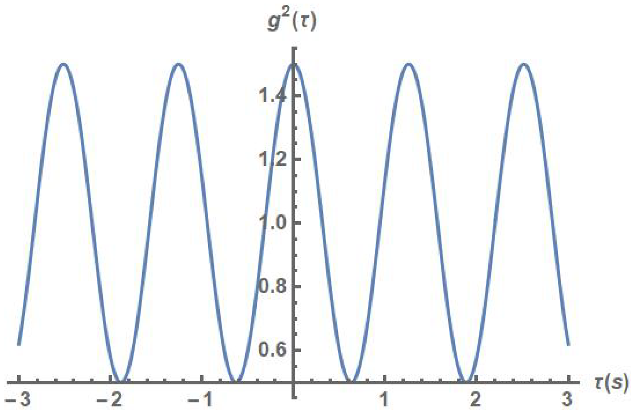
Now that both techniques have been established, a known correlation was analyzed to validate this new technique. An oscillatory signal from Fox [1] was analyzed with both forms of the second order Glauber correlation function. The oscillatory intensity function has the form,

$$I\left(t\right)=I_0(1+A_{0}sin\left(\omega t\right)).$$

(8)

The typical correlation form, Equation (2), gives a function that agrees with the amplitude provided by Fox at $\tau =0$. The closed form solution obtained is:

$$g^2\left(\tau \right)=\frac{1}{2}(2+A_0^{2}cos\left(\omega \tau \right)),$$

(9)

the correlation at $\tau =0$:

$$g^2\left(0\right)=1+\frac{A_0^2}{2},$$

(10)

which agrees with Fox [1]. Using the non intensity weighted correlation from Equation (3), we obtained the following closed form solution,

$$g^2\left(\tau \right)=\frac{4(1+\frac{1}{2}{A}_0^{4}cos\left(\omega \tau \right))}{(2+A_0^2)(2+A_0^{2}cos\left(\omega \tau \right))},$$

(11)

and the correlation at $\tau =0$

$$g^2\left(0\right)=1+\frac{4(1+\frac{3}{2}{A}_0^2)}{{(2+A_0^2)}^2}.$$

(12)

Clearly, Figure 1 and Figure 2 exhibit similar characteristics, with the former having a larger amplitude, though it must be said that both methods when applied to steady periodic functions produce correlations not dependent on time period.

3. Results

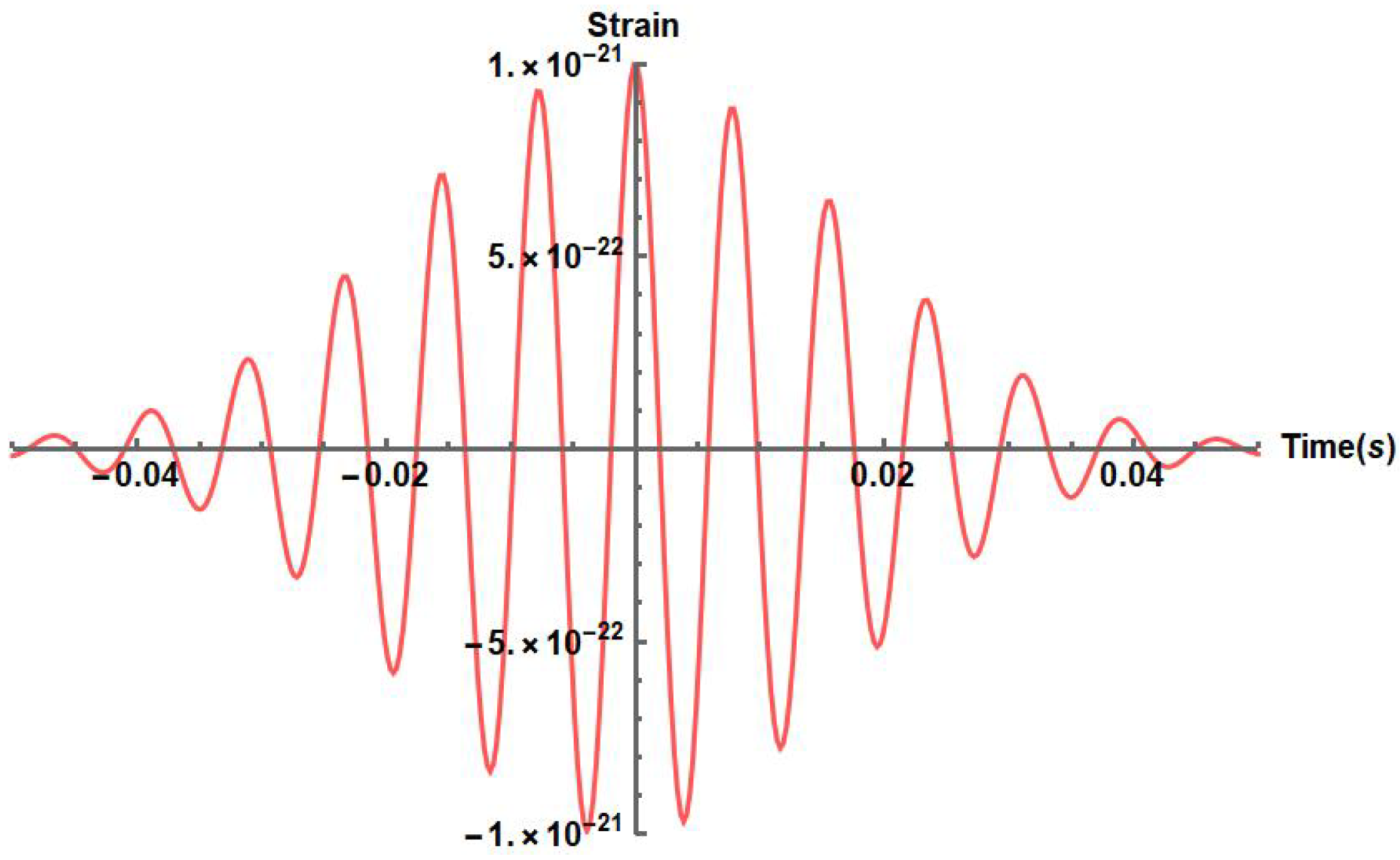
A simplified model of gravitational waves detected at LIGO was approximated using a sine-Gaussian. The correlations of this transient model were observed with both methods. This model was fit by eye to describe the strain amplitude observed at LIGO using three parameters, $\omega ,b,t_m$,

$$h\left(t\right)=h_{max}{e}^{-{\left(\frac{t+t_m}{b}\right)}^2}cos\left(2\pi \omega t\right),$$

(13)

where $t_m$ is the time of the black hole merger, b is a dampening parameter used to fit the function, and $\omega$ is the frequency of the wave, which is assumed to be constant for this simplified model (see Figure 3). The relationship between the strain amplitude (13) and the intensity is shown in (5). Substituting (13) into (11), we obtain a more complicated correlation function than before. The standard time average yields the following closed form solution,

$$g^2(\tau )=\frac{2e^{-\frac{{\tau }^2}{b^2}}T(erf(\frac{T-2t_m-\tau }{b})+erf(\frac{T+2t_m+\tau }{b}))}{b\sqrt{\pi }((erf(\frac{T-2t_m}{\sqrt{2}b})+erf(\frac{T+2t_m}{\sqrt{2}b}))(erf(\frac{T-2(t_m+\tau )}{\sqrt{2}b})+erf(\frac{T+2(t_m+\tau )}{\sqrt{2}b})))},$$

(14)

and the correlation at $\tau =0$

$$g^2(0)=\frac{2T(erf(\frac{T-2t_m}{b})+erf(\frac{T+2t_m}{b}))}{b\sqrt{\pi }{(erf(\frac{T-2t_m}{\sqrt{2}b})+erf(\frac{T+2t_m}{\sqrt{2}b}))}^2}.$$

(15)

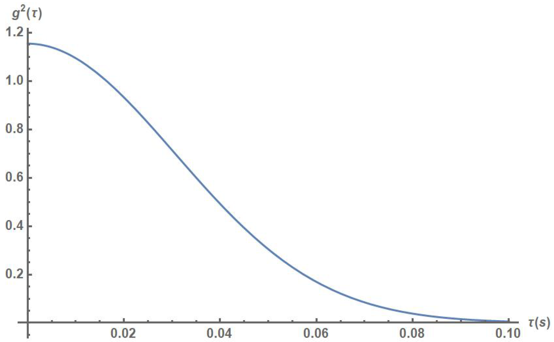
As stated previously, there is evidently a dependence on the time period being averaged over T when looking at the correlation at $\tau =0$, which was not evident for the oscillatory intensity. Using the intensity weighting yields a correlation with no dependence on the period being averaged over. Substituting (13) into (3) yields a more concise correlation,

$$g^2\left(\tau \right)=\frac{2}{\sqrt{3}}{e}^{-\frac{{\tau }^2}{3b^2}},$$

(16)

with $\tau =0$ being

$$g^2\left(0\right)=\frac{2}{\sqrt{3}}.$$

(17)

Both Figure 4 and Figure 5 appear to exhibit a similar characteristic, as $\tau \to \infty$ both $g^2\left(\tau \right)$ s do indeed go to 0. They also have similar behavior around $\tau =0$, with the major difference being the steepness of the correlation.

There are certain properties that electromagnetic waves exhibit when looking at their second order Glauber correlation, and we will compare some of these to our correlation for gravitational waves. The signal in our model is a coherent field undergoing amplitude modulations, although if you look only at the 2nd order Glauber correlations, the functions produced are ambiguous. A chaotic field or a coherent field with amplitude modulations would have been able to produce Glauber correlation functions with similar characteristics to the functions we generated. Some properties are listed below to highlight this ambiguity [1,6,7];

• Coherent light of a single frequency is defined as $g^2\left(\tau \right)=1$;
• For a laser $g^2(\tau =0)=2$ for chaotic light;
• $g^2(\tau =0)>1$ does not necessarily mean the signal is chaotic;
• For chaotic light ${lim}_{\tau \to \infty }{g}^2\left(\tau \right)=0$.

4. Conclusions

A technique for generating 2nd order Glauber correlations using an intensity weighting was discussed, which produced comparable results to the time-averaging technique for both an oscillatory intensity and a transient signal. A sine-Gaussian was introduced to be used as a simplified model of the first signal detected by LIGO. This model was then analyzed with both methods for calculating the correlation, and produced functions that exhibit both chaotic and coherent amplitude modulated signal correlation functions.

References

- Fox, M. Quantum Optics—An Introduction; Oxford University Press: Oxford, UK, 2006. [Google Scholar]
- Louden, R. The Quantum Theory of Light, 3rd ed.; Oxford University Press: Oxford, UK, 2000. [Google Scholar]
- Baym, G. The physics of Hanbury Brown-Twiss intensity interferometry: From stars to nuclear collisions. Acta Phys. Pol. B 1998, 29, 1839–1884. [Google Scholar]
- Facao, M.; Lopes, A.; Silva, A.L.; Silva, P. Computer simulation for calculating the second-order correlation function of classical and quantum light. Eur. J. Phys. 2011, 32, 925. [Google Scholar] [CrossRef]
- Sathyaprakash, B.S.; Schutz, B.F. Physics, Astrophysics, and Cosmology, with Gravitational Waves. Living Rev. Relat. 2009, 12, 1–141. [Google Scholar] [CrossRef] [PubMed] [Green Version]
- Lebreton, A.; Abram, I.; Braive, R.; Sagnes, I.; Robert-Philip, I.; Beveratos, A. Theory of Interferometric Photon-Correlation Measurements: Differentiating Coherent from Chaotic Light. Phys. Rev. A 2013, 88, 013801. [Google Scholar] [CrossRef] [Green Version]
- Wikipedia Contributors. Degree of Coherence. Wikipedia, the Free Encyclopedia. Available online: https://en.wikipedia.org/w/index.php?title=Degree_of_coherence&oldid=1001227113 (accessed on 30 January 2021).
Figure 3.
Model gravitational wave waveform from Equation (13).
Publisher’s Note: MDPI stays neutral with regard to jurisdictional claims in published maps and institutional affiliations. |
© 2021 by the authors. Licensee MDPI, Basel, Switzerland. This article is an open access article distributed under the terms and conditions of the Creative Commons Attribution (CC BY) license (https://creativecommons.org/licenses/by/4.0/).
Share and Cite
MDPI and ACS Style
Barrett, A.; Jones, P. Second Order Glauber Correlation of Gravitational Waves Using the LIGO Observatories as Hanbury Brown and Twiss Detectors . Phys. Sci. Forum 2021, 2, 25. https://doi.org/10.3390/ECU2021-09519
AMA Style
Barrett A, Jones P. Second Order Glauber Correlation of Gravitational Waves Using the LIGO Observatories as Hanbury Brown and Twiss Detectors . Physical Sciences Forum. 2021; 2(1):25. https://doi.org/10.3390/ECU2021-09519
Chicago/Turabian StyleBarrett, Alexander, and Preston Jones. 2021. "Second Order Glauber Correlation of Gravitational Waves Using the LIGO Observatories as Hanbury Brown and Twiss Detectors " Physical Sciences Forum 2, no. 1: 25. https://doi.org/10.3390/ECU2021-09519