Dynamic Lifecycle Cost Modeling for Adaptable Design Optimization of Additively Remanufactured Aeroengine Components

Abstract

Additive manufacturing (AM) is being used increasingly for repair and remanufacturing of aeroengine components. This enables the consideration of a design margin approach to satisfy changing requirements, in which component lifespan can be optimized for different lifecycle scenarios. This paradigm requires lifecycle cost (LCC) modeling; however, the LCC models available in the literature consider mostly the manufacturing of a component, not its repair or remanufacturing. There is thus a need for an LCC model that can consider AM for repair/remanufacturing to quantify corresponding costs and benefits. This paper presents a dynamic LCC model that estimates cumulative costs over the in-service phase and a nested design optimization problem formulation that determines the optimal component lifespan range to minimize overall cost while maximizing performance. The developed methodology is demonstrated by means of an aeroengine turbine rear structure.

1. Introduction

Suppliers of aeroengine components are operating in an increasingly uncertain product development environment. The need to design more efficient aeroengines is driving manufacturers to shorten development time. This means that suppliers have to initiate their design work long before mature requirements are available [1]. As a result, there is a high probability that requirements will change not only during the design process but also during operation. This has a significant impact on design targets related to the lifespan of components in future aircraft programs.

While components are typically designed for a required lifespan of about 30 years, there is growing interest from customers to increase lifespan due to economical and environmental factors. For example, the resale of aircraft among airlines introduces new lifespan requirements that need to be satisfied during the aircraft’s re-certification process [2]. One example is the Boeing 737-200, which made its first commercial flight in 1970 for Air California [3]. Although the airline is not operating anymore, its aircrafts continue their service after several resales. Lifespan extensions are also occurring in military aircrafts. The B-52H fleet is likely to be in operation for nearly 100 years as the U.S. Air Force is committing to flying the aircraft into the 2050s [4]. This means that aircrafts are going to be in operation for a longer time than what they were designed for.

Another reason for extending the lifespan requirement is growing demand from customers for sustainable products [5]. In response to these demands, manufacturers are increasingly interested in applying circular economy (CE) strategies, which aim at maintaining products in the economy for as long as possible [6,7,8]. One way of adopting a CE strategy is to extend the lifespan of the component through upgrades and re-certification [9].

Finally, unforeseen events, such as the ongoing Covid-19 pandemic, can alter the aviation business dramatically, emphasizing the need to assess alternative lifecycle scenarios and find new ways to utilize equipment. From a design perspective, these changes in lifespan requirements can become a true source of corrective reworks and schedule delays. That is because suppliers would start the development work based on immature input requirements regarding lifespan. Therefore, there is a growing interest to develop aeroengine components that already take into account the possible life extensions that could occur during the life of an aircraft.

One possible way to meet changing lifespan requirements in aerospace components is by increasing design margins [10]. This results in robust component designs that allow accommodating a wide range of lifespan requirements provided the anticipated changes are compliant with engine certification. However, this strategy typically results in over-designing components, which negatively impacts performance (e.g., through increased weight) and manufacturing costs. An alternative approach is to design a component based on a preliminary lifespan and to modify the geometry as soon as requirement changes occur.

This alternative can be made possible using additive manufacturing (AM), which enables material deposition on existing components [11]. Using AM, the initial design geometry can be adapted during the development and operation stages [12]. However, this strategy has drawbacks too. If the changes in lifespan requirements are too many or unforeseen, the cost of such modifications could overcome the cost of adopting a robust component design with high design margins. Providing aeroengine suppliers with a modeling approach that optimizes the impact of AM-adapted designs on lifecycle cost (LCC) can be helpful and effective.

This paper presents a modeling approach to assist in design decisions based on a cost-benefit analysis of different component design strategies. A dynamic LCC model is developed to estimate costs over a component’s lifecycle while considering its remanufacturing by direct energy deposition (DED), the most commonly used AM process in the repair/remanufacturing of products because of its ability to restore metal-based parts in a layer-by-layer manner [13]. The LCC model is used in solving an optimization problem for determining the optimal range of component design lifespan to minimize lifecycle cost while maximizing performance. The proposed methodology enables designers to assess geometric adaptability (introduced by AM deposition) to accommodate changes in lifespan requirements.

1.1. Changing Lifespan Requirements

Various factors can influence a component’s lifespan. Here, we distinguish between internal and external factors. Internal factors are controllable during the design process and can alter degradation mechanisms impacting structural integrity. External factors cannot be controlled by the designer but impact functionality, cost, and performance. They account for uncertainties that originate from consumer behavior as well as issues such as changes in legislation and aircraft operation profile and maintenance strategies.

Several studies have been published on consumers’ behavior throughout the in-service phase [14,15,16]. These studies are mainly survey-based. Results showed that consumers are requesting products that live longer through the continuous restoration of the product’s value. Typical drivers for restoration are cost efficiency and environmental friendliness of the product, hence promoting a transition to circular economies [17]. One way to achieve this is through repair/remanufacturing in a cost-efficient manner. Other factors such as the effect of waste management policies on consumers’ decisions to recycle, reuse, dispose of, or store different components were investigated [14]. Although component repair and recovery can be the most favorable from an environmental and economical perspective, the lack of manufacturers responsibility and the user practice of airlines are considered as major barriers preventing repair from becoming the dominant end-of-life (EOL) option [18]. While customer preferences for different EOL strategies have been a major point of interest in the literature, there is a lack of research investigating costs associated with recovery strategies. In the aerospace industry, it is quite challenging to determine accurately the optimal design lifespan at early stages of product development. This is due to the complexity of aircraft systems and the high degree of functional and physical integration involved. As a result, there is a high degree of uncertainty associated with lifespan requirements. A common way of managing changes in the lifespan requirement of an aerospace component is by performing additional low-cycle fatigue (LCF) analysis and considering updated and more precise load cases based on components tested in-service.

1.2. Adaptability and Robustness

The terms adaptability and flexibility are used interchangeably in the literature to refer to a system’s property that allows it to respond to requirement changes occurring after the system is in operation in a timely and cost-effective manner [19,20]. In order to eliminate confusion between design flexibility and adaptability, Ross et al. made a distinction between adaptability and flexibility through the location of the change agent [21]. A change agent is defined as the force that brings about the change. If the change agent is external to the system, then the change under consideration is a flexible-type change. If the change agent is internal to the system, then it is an adaptable-type change. In general, flexibility tends to be challenging to assess and quantify as it deals with a system’s ability to respond to scenarios that may never have been envisioned by the designers.

We adopt the above-mentioned distinction between adaptability and flexibility and focus on adaptability induced by additive remanufacturing in aeroengine components. Some researchers quantify adaptability by proposing a metric based on a component’s option value (OV), defined as the difference between the gain in value after the component is upgraded and the expected present cost of upgrading [20,22].

Robustness, on the other hand, is a separate design characteristic. Although both robustness and adaptability refer to the ability of a system to handle change, there is a difference between the nature of change and the system’s reaction to change in each case. Adaptability implies the ability of a design to satisfy changing requirements, whereas robustness involves satisfying a fixed set of requirements despite changes in the system’s environment or within the system itself [12]. Figure 1 illustrates schematically these three different design approaches. P1 and P2 are two different time periods during the component’s lifespan. P1 is defined as the initial time period during which the component design occurs and P2 as a time period during which changes in the required lifespan occur. As shown in Figure 1, traditional design approaches favor designs that are optimized to satisfy original requirements (point-optimal design). Over time, these requirements might change resulting in a performance gap. Uncertainty regarding future requirements makes it difficult to design for required design changes. One way of tackling this uncertainty in requirements is through adopting a robust component design. This will reduce the performance gap resulting from changes in requirements however will introduce a performance gap at the initial period due to the over-design of the component. Therefore, an alternative approach is to consider an adaptable component design. The chosen design characteristics may not be justified in the context of optimizing the system for the initial set of requirements, however, these characteristics will allow the system to evolve as requirements change during operation, reducing the performance gap (see Figure 1).

Through integrating adaptability in design, several options are made available, such as the option to service for life extension or to upgrade. These options do not need to be set in the initial design, they can be exercised after the aircraft is in operation, depending on how events unfold. Most studies reported in literature address adaptability introduced by modularity [23,24]. A product can be designed, redesigned, upgraded, produced, and outsourced more easily when it is divided into relatively independent modules. However, for highly integrated components, classical modular approaches are not possible [25]. In addition to modularity, AM has the potential to increase a component’s adaptability through altering the existing product geometry by adding material to adjust its shape and dimensions. Despite this, fundamental questions of applicability and cost-effectiveness of introducing design adaptability by AM remain unanswered. To answer these questions, a comprehensive LCC model is needed to perform a cost-benefit analysis.

2. Background

In 2014, Siemens first reported the use of AM in the repair of gas turbine components [26]. Since then, several studies focused on the potential of utilizing AM in repair, refurbishment, and remanufacturing [5,27,28]. These studies consider mostly structural and mechanical properties. Applications are limited to expensive components that endure severe operating conditions and have complex structures and requirements. The benefits of repairing such components instead of replacing them were recognized readily. Moreover, platforms were proposed to allow automated process planning for combined additive and subtractive processes [29,30]. The goal is to improve the surface quality and shape accuracy of the final product. Process planning was performed based on process characteristics, technological requirements, and available resources. Other studies focused on defining product characteristics that impact remanufacturability by AM [31].

2.1. Lifecycle Cost Models for Additively (Re)manufactured Components

Lifecycle cost is also referred to as whole life cost or lifetime cost depending on the industry sector in which the term is being used. It determines the cost-effectiveness of a design by considering all stages throughout the life of a product or system, from conceptual design to disposal. Depending on the product or system, different elements can be considered in its LCC calculation. For example, LCC estimation of a highway pavement considers different cost elements than those of an aeroengine component. Several cost models of varying level of accuracy and complexity exist in the literature.

During the past decade, studies on costs associated with AM gained the attention of many researchers. Most studies aimed at comparing the energy consumption, emissions saving, and costs of subtractive and additive manufacturing processes [16,31,32,33,34]. Other researchers developed models to perform an inter-process cost comparison between different AM process types [35]. Reviewing the evolution of AM cost models, Hopkinson and Dickens were the first to analyze AM costs [36]. Initially, the technology was mainly used for rapid prototyping (RP). Over time, interest of using AM in production has increased. Models were then developed that use rough estimates of machine costs, labor costs, and material costs [36]. These were later improved through considering large production volumes, overhead costs, and material recycling [37]. In 2012, the concept of time-driven activity-based costing (TDABC) was introduced and adopted for AM cost estimations [38,39,40,41]. Time-driven signifies that the allocation depends on the duration of the activities. These studies were the first to examine in detail the economic and energy-related aspects as well as the time necessary to realize AM-based production. The obtained results were used to rate different cost drivers associated with AM processes.

Other studies focused on business models that include activities relevant to pre- and post-processing costs [42,43,44]. Bauer and Malone proposed the use of regression analysis based on data of similar systems to allow the development of cost estimating relationships (CERs) [45]. Experiments were carried out to estimate manufacturing costs with different build scenarios and machine utilization [46]. Results showed that manufacturing time per part is the key factor to optimize the costs of laser AM. Fera et al. analyzed AM from an operations management point of view taking into account availability, performance, and quality loss [47]. A cost estimation model was developed in [48] to assist decision-makers in comparing between traditionally manufactured parts and their AM counterparts. This was achieved by providing a break-even point where the total LCC for both components are equal. Such break-even values can then be used to determine whether or not to opt for AM.

While the predictive capability of LCC models increases as more stages in the life of a part are considered, there is a need to estimate the effective costs associated with additive remanufacturing. Since this requires an analysis over the lifecycle, some recent LCC modeling efforts focused on using a system dynamics (SD) approach [49,50]. System dynamics models can be used to capture information flow and feedback [51]. The decision-maker can thus model a variety of scenarios and observe system performance under different conditions. SD is well suited for modeling continuous processes, systems where behavior changes in a non-linear fashion, and systems within which extensive feedback occurs. As a matter of practice, SD is often used in strategic policy analysis.

2.2. Lifecycle Cost Optimization

In response to industry needs, manufacturers aim at optimizing designs to improve reliability while reducing operation costs. Pelzeter was the first to combine the terms LCC and optimization [52]. His work focused on the optimization of different building designs with respect to LCC-based rankings. Du et al. developed an optimization model to assist designers in choosing a suitable LCC methodology [53]. The objective was to minimize a weighted sum of the mean LCC and its standard deviation. Another framework was proposed to study the impact of design on lifecycle analysis (LCA) [54]. Optimization was integrated into the framework to minimize the product’s environmental impact due to the use of AM processes. Wu et al. proposed an approach for design optimization of plastic injection tooling (mold) using a thermo-mechanical finite element model [55].

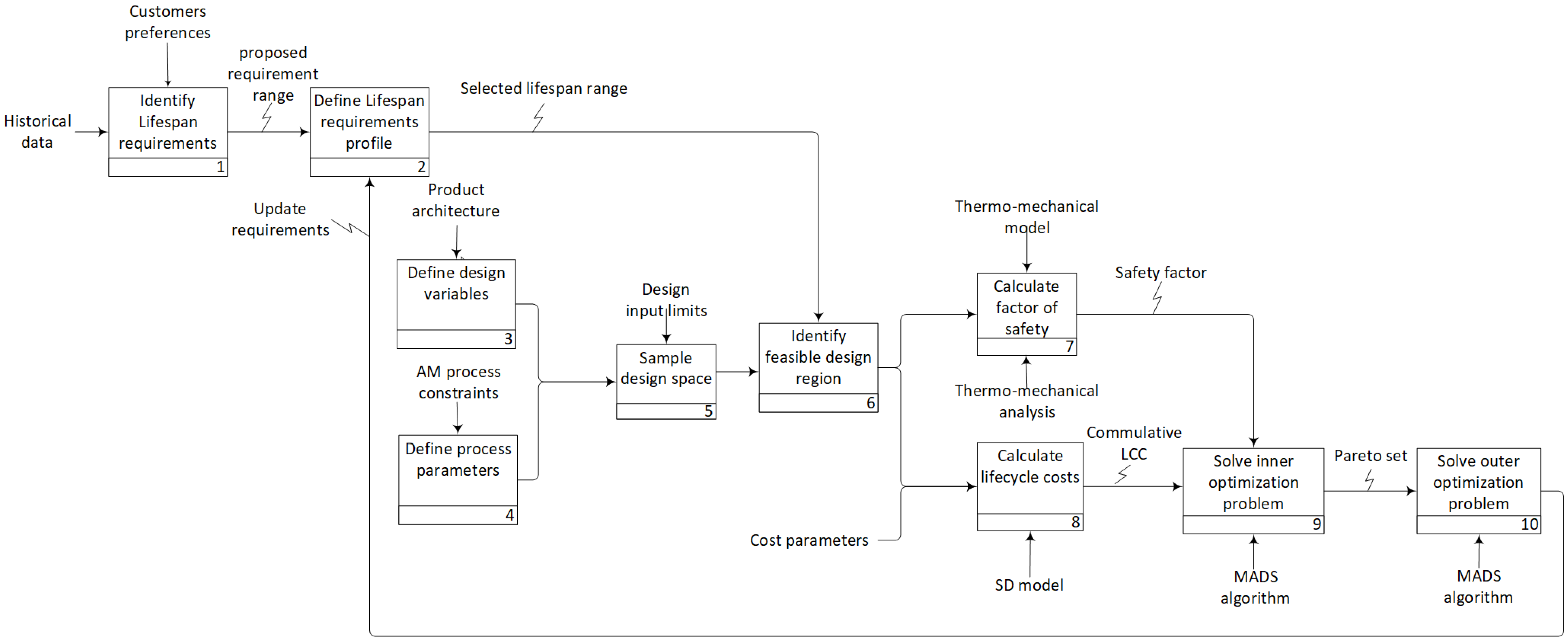
3. Proposed Methodology

The model presented in this paper is the result of a collaboration with a supplier of aeroengine components. The interest of the industrial partner is motivated by the fact that altering a component geometry by AM once it is in operation requires extra activities such as undergoing re-certification to ensure that it is safe and that it meets new lifespan requirements. This implies additional costs that may outweigh costs associated with a robust design strategy in which margins are added. Therefore, a good design strategy should balance the trade-off between robustness and adaptability so that LCC is minimized while performance is maximized.

The methodology is based on integrating a dynamic LCC model with a nested optimization approach. The model allows the assessment of an alternative mean-of-life extension that uses AM to adapt component geometry during operation. Figure 2 provides a flow diagram in which the starting point is to select the required component lifespan range based on historical data and customer preferences. The selected range is used as an input to an optimization problem that determines the Pareto set of design alternatives associated with the bi-objective problem of minimizing LCC and maximizing performance, where a factor of safety is used to represent the latter. It is estimated based on results obtained using the thermo-mechanical analysis model presented in [56].

Suppliers of aerospace components cannot predict during the preliminary design phase whether customers will prefer to extend the life of a component (rather than just replacing it with a new one) and to what extent this life extension would be. As described in the introduction, these choices are largely dependent on economic factors and the customer’s desire for more durable products.

We make the assumption that the customer may decide at any point in a component’s lifespan whether it is economically efficient to extend the life of the component or to replace it. Therefore, the LCC of both options is evaluated continuously throughout the component’s lifetime so that the option presenting the lowest LCC can be determined at any time. Let us consider for example the highly volatile fuel price. In a market with high fuel prices, a heavy component with high design margins may imply higher LCC compared to a lighter component which is adapted and extended multiple times throughout its lifecycle. Conversely, if the fuel prices are low, a robust design with high margins that does not require life extension may be the preferred option.

In addition, different geometries of the AM deposited part can be considered at different times throughout the in-service phase extending the lifespan accordingly. To that end, the model used in [9,57] is expanded by treating the required component lifespan as an optimization variable for which the LCC of different component designs is evaluated. The LCC model is then used in a nested optimization problem to determine if, when, and how a component can be remanufactured throughout the in-service phase. The next section demonstrates the proposed methodology by means of an aeroengine turbine rear structure (TRS) design example, for which a dynamic LCC model is developed and used.

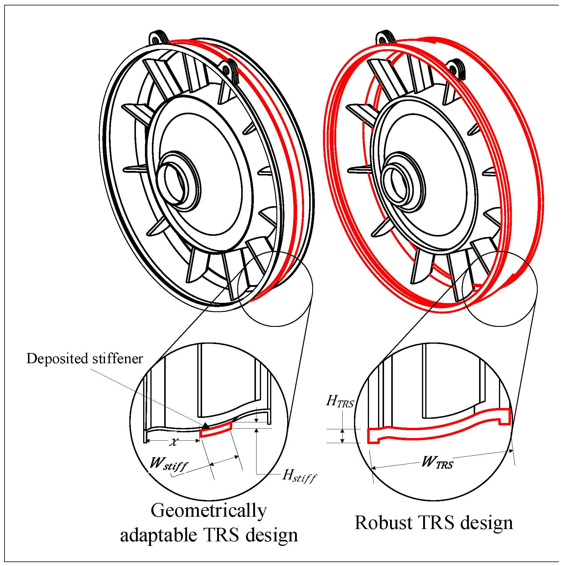
Additively Deposited Stiffener on an Aeroengine Turbine Rear Structure

One possible strategy to adapt to changing lifespan requirements is to extend the life of a TRS by additive deposition of a circumferential stiffener on its shroud. Figure 3 depicts the geometrical configuration of the TRS and the deposited stiffener along with the corresponding design optimization variables considered in this study.

The design problem considers the parent component geometry, the deposited stiffener geometry, an AM process parameter, and the time throughout the in-service phase at which the stiffener is deposited. Note that the proposed methodology is applicable to both existing and newly designed components.

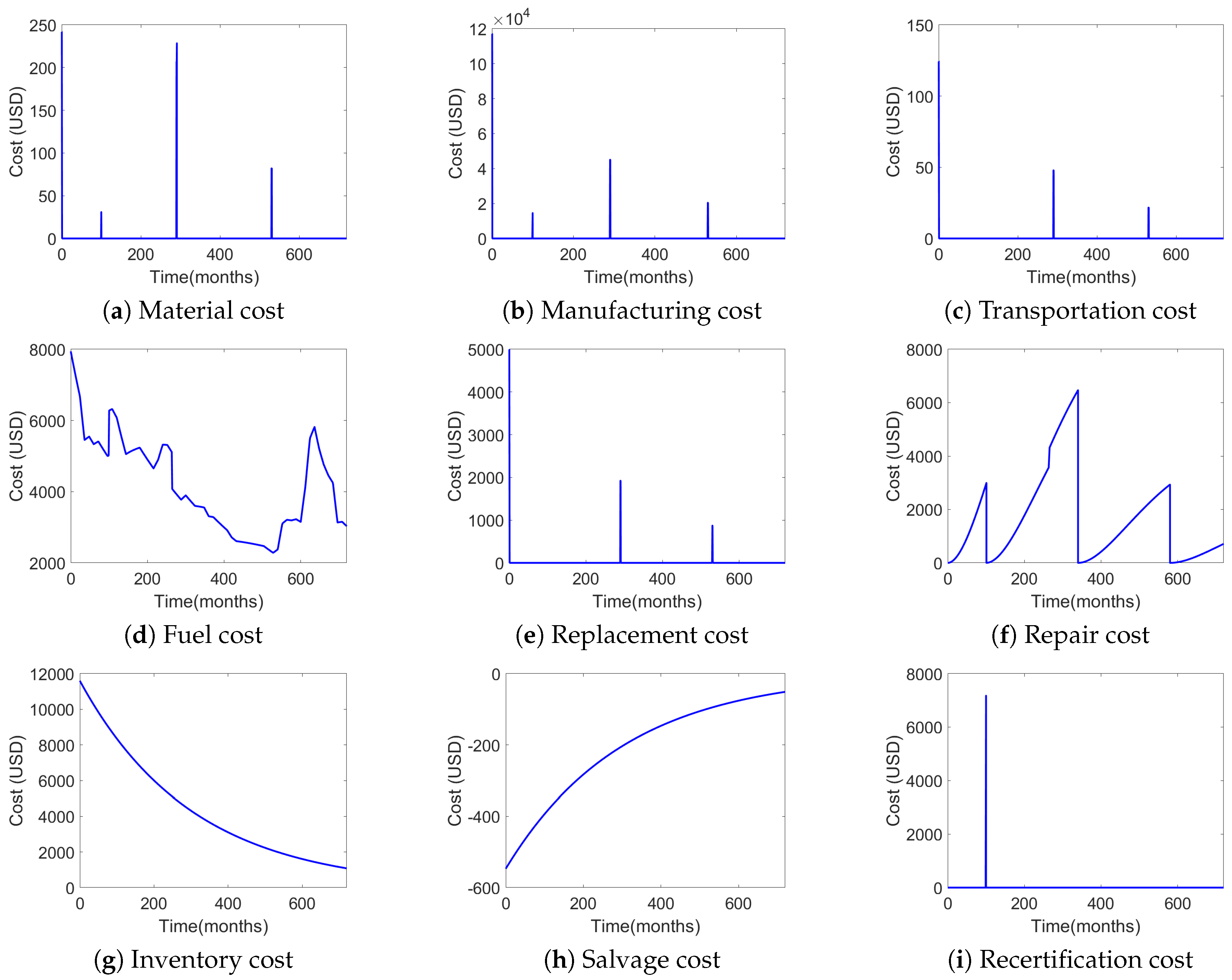
3.1.1. Lifecycle Cost Model

The present value (PV) of the LCC (denoted by $V_P$) is used to discount all future costs:

$$V_P=\sum _{t=0}^{N_T}\frac{C_t}{{\left(1+r\right)}^t},$$

(1)

where $C_t$ is the sum of costs in year t, r is the discount rate, and $N_T$ is the in-service period. While most published research focuses on purchasing and production costs, a deeper understanding of costing structures is required. This is because AM has a significant impact on many aspects of the production and operations chain. The main categories considered in the proposed LCC model are discussed below along with the relationships used to estimate associated costs. Most of these are adopted from [9] and modified to accommodate changes in component lifespan over time.

Material cost is given by

$$C_1\left(t\right)={\alpha }_{mat}{W}_{total},$$

(2)

where ${\alpha }_{mat}$ is the monthly price of Inconel 718 per weight obtained from historical data recorded over 30 years [58]. It is assumed that the same price trend will occur. Cyclic repetition of the price data was used to estimate prices over a wider time range. $W_{total}$ is the sum of the TRS component weight ($W_{TRS}$) and deposited stiffener weight ($W_{stiff}$) calculated from their corresponding volume and material density. The associated plot in Figure 4 displays material costs introduced at every component replacement process during the in-service period along with material costs associated with the stiffener deposition. All costs are discounted to their present value.

Manufacturing cost is given by

$$C_2\left(t\right)={\beta }_{man}(LS+LE)+{\gamma }_{man},$$

(3)

where ${\beta }_{man}$ is the manufacturing cost per cycle and ${\gamma }_{man}$ is a fixed cost accounting for machine tooling costs. Variable costs are assumed to be linearly proportional to the number of cycles the TRS can achieve. “Per cycle” cost estimation is used as it reflects the TRS design lifespan (assuming 1460 flying cycles per 12 months) and geometry. This in turn impacts the manufacturing time, required labor, and machine maintenance, which are components of the manufacturing cost [59]. $LS$ and $LE$ are the component’s design lifespan and life extension due to the deposited stiffener respectively. $LS$ is linearly interpolated using 82 months for a TRS with 11 Kg outer shroud and 329 months for a TRS with 78 Kg outer shroud. $LE$ is estimated using the thermo-mechanical analysis developed by Al-Handawi et al. to model and evaluate the additive deposition process [56]. As displayed in Figure 4, manufacturing costs show a similar trend to that of material costs but with significantly higher values.

Transportation cost is given by

$$C_3\left(t\right)={\alpha }_{trans}{W}_{TRS},$$

(4)

where ${\alpha }_{trans}$ is the transportation cost per unit weight. These account for costs associated with the transportation of a new TRS to the operation site in order to replace an old TRS. The additive deposition of a stiffener is done on site throughout the service period in response to changes in requirements. Transportation costs are only applicable during component replacement activity and not during on-site component remanufacturing. Therefore, the combined weight of the TRS and the deposited stiffener $W_{total}$ does not impact cost.

Fuel cost is given by

$$C_4\left(t\right)={\alpha }_{fuel}(LS+LE)W_{total},$$

(5)

where ${\alpha }_{fuel}$ is the fuel price per weight. As future fuel price prediction is outside the scope of this paper, historical annual price data recorded over 80 years interval was used assuming that fuel prices will follow the same trend. In order to obtain monthly fuel prices from the available annual price data, we linearly interpolated data between years [60]. Moreover, it is assumed that 0.029 gallons of fuel are consumed per kg weight per engine cycle. Results show non-linear behavior of fuel prices over time and an increase in fuel consumption after the stiffener deposition due to the added weight.

Replacement cost is given by

$$C_5\left(t\right)={\gamma }_{repl},$$

(6)

where ${\gamma }_{repl}$ is the constant cost of service labor to install a new TRS.

Repair cost is based on Thomsen et al. [9]:

$$C_{6i}\left(t\right)=\frac{\$1.41[1-e^{-K(t/\lambda )}]}{cycle}.$$

(7)

Assuming the TRS use phase is 1460 flying cycles per year, the above equation is rewritten as

$$C_6\left(t\right)=\frac{\$173[1-e^{-K(t/\lambda )}]}{month},$$

(8)

where K = 2 and $\lambda$ = $LS(-ln{\left(0.9\right)}^{-\frac{1}{K}})$. Repair costs are linearly interpolated and proportional to the probability of failure and calculated in terms of US dollars per month. The present value of repair costs increases exponentially towards the end of a component’s design lifespan. As shown in Figure 4, component remanufacturing during operation reduces repair costs throughout its remaining useful life.

Inventory cost is given by

$$C_7\left(t\right)={\alpha }_{inv}{W}_{TRS}+{\beta }_{inv}LS+{\gamma }_{inv},$$

(9)

where ${\alpha }_{inv}$ is a constant representing material cost at the TRS fabrication time, ${\beta }_{inv}$ is the cost per designed TRS cycle, and ${\gamma }_{inv}$ is a constant representing the cost of depot labor. The values used for ${\alpha }_{inv}$, ${\beta }_{inv}$, and ${\gamma }_{inv}$ are listed in

Table 1. Lifecycle cost model parameter values.

Symbol	Value	Units
${\rho }_{mat}$	0.0082	kg/cm${}^3$
r	4	%
L	380	cm
${\gamma }_{\mathrm{man}}$	20,000	USD
${\beta }_{\mathrm{man}}$	3.33	USD/cycle
${\alpha }_{\mathrm{trans}}$	4	USD/kg
${\gamma }_{\mathrm{repl}}$	5000	USD
${\alpha }_{\mathrm{inv}}$	5	USD/kg
${\beta }_{\mathrm{inv}}$	0.166	USD/cycle
${\gamma }_{\mathrm{inv}}$	1000	USD
${\alpha }_{\mathrm{disp}}$	100	USD
${\beta }_{\mathrm{disp}}$	12	USD/kg
${\gamma }_{\mathrm{recert}}$	9977	USD

. They are adopted from Thomsen et al. [9] and were obtained from subject matter experts (SMEs) at GKN Aerospace Engine Systems Sweden for the specific TRS case study. Inventory cost considered in the cost model is a function of the properties of available spare parts. Inventory cost is assumed constant throughout the desired service period, therefore its present value depreciates over time.

Salvage cost is given by

$$C_8\left(t\right)={\alpha }_{disp}-{\beta }_{disp}{W}_{total},$$

(10)

where ${\alpha }_{disp}$ is the disposal cost per TRS and ${\beta }_{disp}$ is the price per weight of scrap metal sold. Salvage cost results displayed in Table 4 show negative cost values indicating that the income from this cost category is greater than the cost.

Recertification cost is given by

$$C_9\left(t\right)={\gamma }_{recert},$$

(11)

where ${\gamma }_{recert}$ is the fee of issuing a supplemental type certificate for propulsion turbine engines with take-off thrust over 25 KN according to the European Union Aviation Safety Agency [61].

Figure 4 depicts sample results for each cost category over the desired service period of 700 months. In the displayed results, the TRS shroud width and thickness are assumed 20 cm and 0.5 cm, respectively. The calculated design lifespan is 240 months. Moreover, it is assumed that a stiffener with 5 cm width and 0.2 cm thickness is additively deposited at the 100th month of operation, causing a life extension of 50 months.

The total present value of the LCC per year is calculated by adding all nine cost components (cf. Figure 5a). An assumption is made that AM remanufacturing is performed only one time throughout the in-service phase; in the example used here, this happens at month 100 (first peak). The other peaks reflect costs associated with replacement processes occurring at the end of the product’s design life. The presented model considers the scenario where the entire TRS is replaced at the end of its lifespan. The TRS is repaired by AM if there is a change in requirements. While repairing the TRS by AM extends its lifespan, it is replaced at the end of the latter. Therefore, the lifespan of the TRS depends on its initial design parameters and whether it is repaired by AM. However, due to the value of the considered in-service period (700 months) and the assumption that AM remanufacturing is performed only once throughout the in-service phase, several TRS replacements may be required. The cumulative LCC over time is shown in Figure 5b. The final value at the end of the desired service period is used as the objective to minimize in the optimization problem.

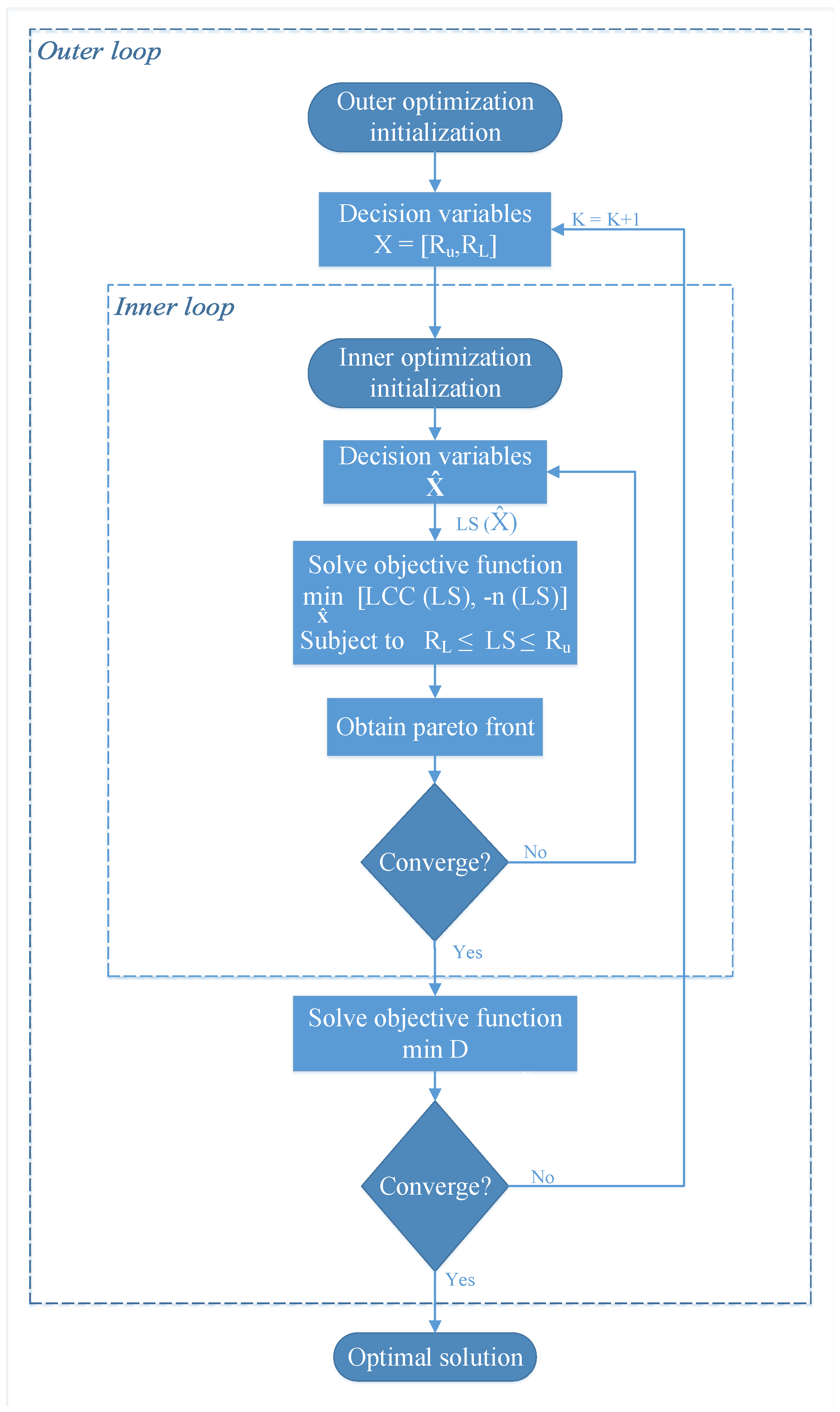
3.1.2. Optimization Problem Formulation

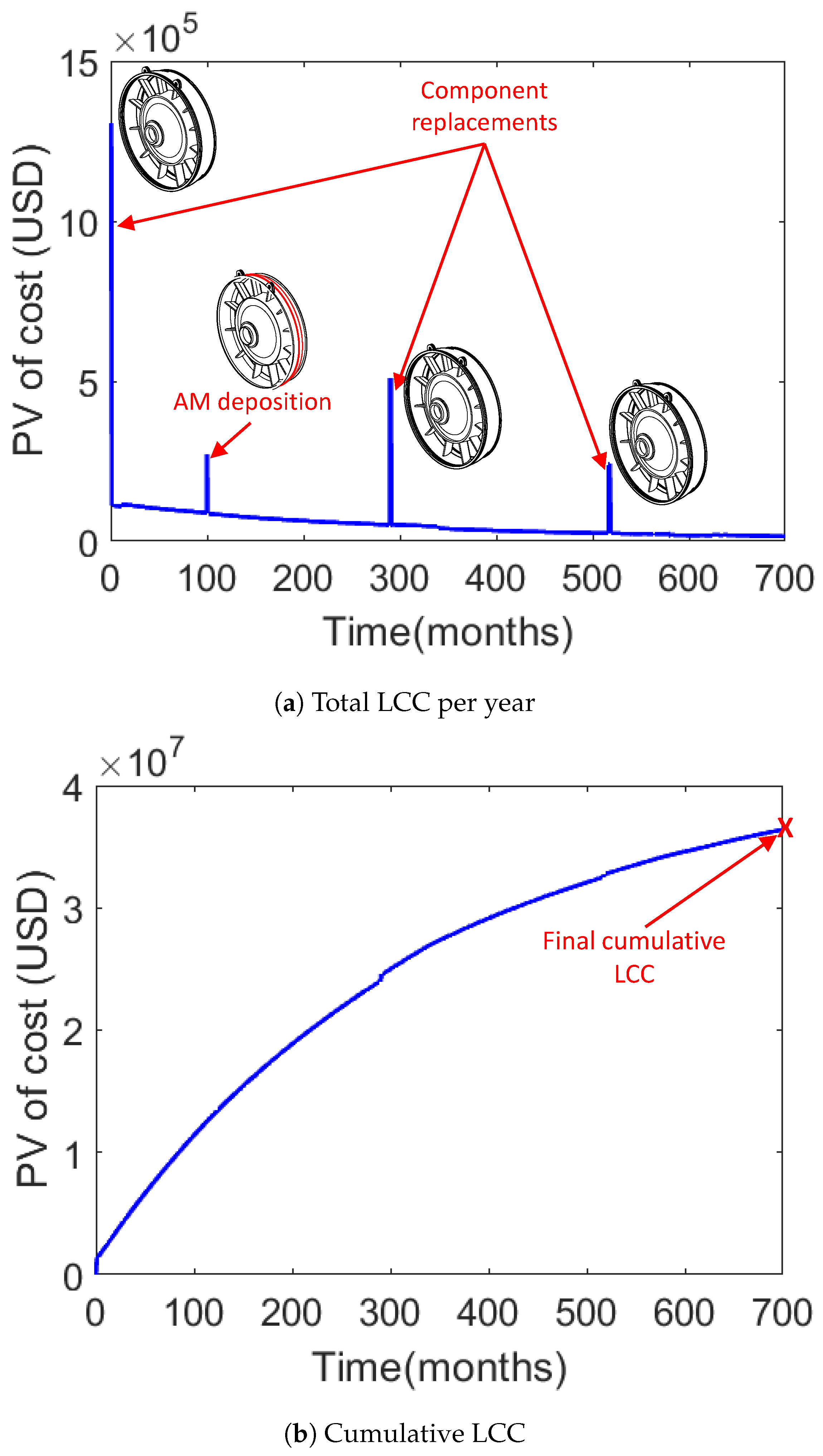
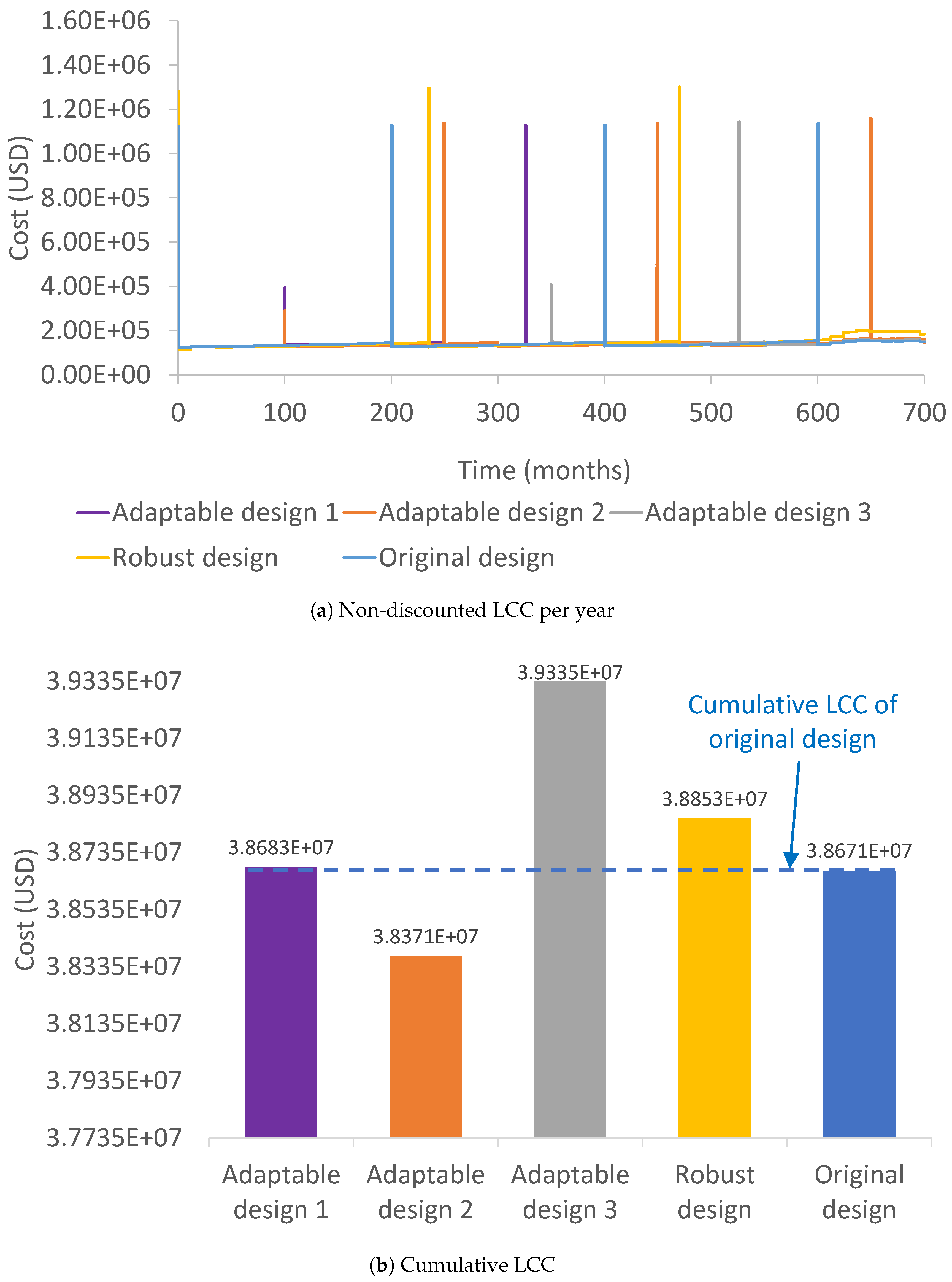
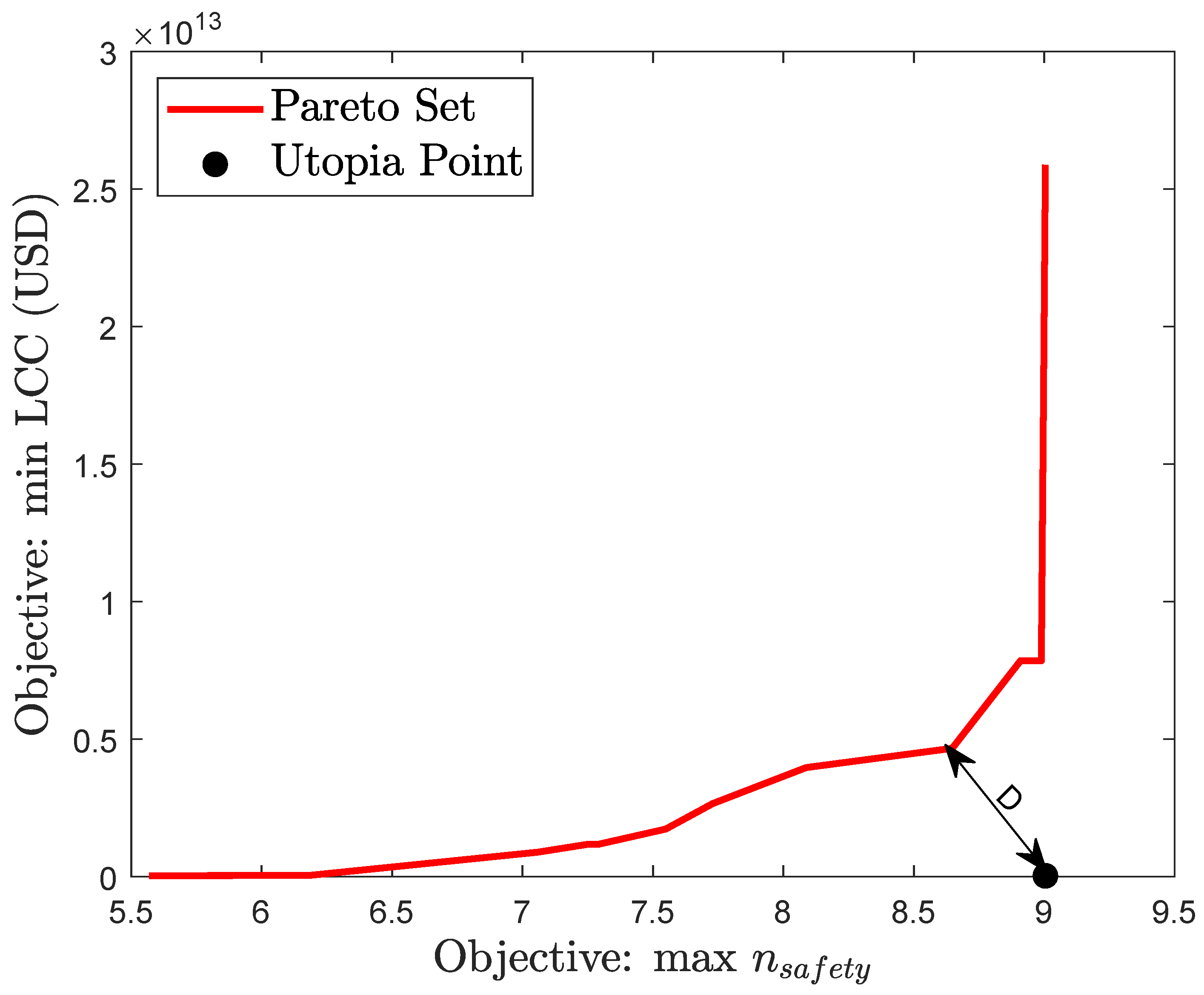
A nested optimization strategy is used to integrate component and stiffener design optimization with lifespan requirement optimization. The proposed methodology assists designers in selecting an optimum lifespan range to be used as a requirement in early design stages. The flow diagram of the optimization process is shown in Figure 6.

An inner optimization problem is solved to obtain design solutions that minimize LCC and maximize performance. Since there is a trade-off between LCC present value ($V_P$) and safety factor (n), a set of Pareto-optimal solutions is generated. The purpose of the outer loop is to determine values of the lower and upper bounds of the required lifespan range. This is achieved through solving an optimization problem to minimize the distance between the utopia point and the Pareto front generated by the inner optimization loop.

The inner bi-objective optimization problem is formulated as

$$\begin{array}{ccc}\underset{\widehat{x}}{\mathrm{minimize}}\hfill & \hfill & [V_P\left(\widehat{x}\right)-n\left(\widehat{x}\right){]}^T\hfill \\ \mathrm{subject}\mathrm{to}\hfill & \hfill & x+W_{stiff}-W_{TRS}\le 0\hfill \\ \hfill & \hfill & W_{stiff}{H}_{stiff}-0.1W_{TRS}{H}_{TRS}\le 0\hfill \\ \hfill & \hfill & LS\left(\widehat{x}\right)\le R_U\hfill \\ \hfill & \hfill & R_L\le LS\left(\widehat{x}\right),\hfill \end{array}$$

(12)

where $\widehat{x}=[x,W_{\mathrm{TRS}},H_{\mathrm{TRS}},W_{\mathrm{stiff}},H_{\mathrm{stiff}},L_{\mathrm{p}},N]$.

The constraints ensure that the deposited stiffener is contained within the limits of the TRS shroud and that the deposited stiffener weight does not exceed 10% of the parent component weight. The bounds on the component lifespan (which is a function of the design optimization variables) are determined at the outer optimization problem. An ensemble of surrogates is constructed and used based on data obtained from the thermo-mechanical analysis model to facilitate an efficient optimization process [62]. The dynamic LCC model was implemented using the Matlab Simulink toolbox. The optimization problems are solved using the Mesh Adaptive Direct Search (MADS) algorithm [63].

Table 2. Design optimization variables for inner optimization problem.

Variable	Symbol	Units	Lower Bound	Upper Bound
Stiffener axial position	x	cm	4.5	15.5
TRS shroud width	$W_{\mathrm{TRS}}$	cm	18	25
TRS shroud thickness	$H_{\mathrm{TRS}}$	cm	0.2	1
Stiffener width	$W_{\mathrm{stiff}}$	cm	2	15.5
Stiffener thickness	$H_{\mathrm{stiff}}$	cm	0.2	2
AM laser power	$L_{\mathrm{p}}$	W	3500	4500
Deposition year	N	months	60	640

summarizes the design optimization variables used in the inner optimization problem along with their bounds.

The outer optimization problem is formulated as

$$\begin{array}{cc}\underset{\check{x}}{\mathrm{minimize}}\hfill & D\hfill \\ \mathrm{subject}\mathrm{to}\hfill & R_U-R_L-120\le 0\hfill \\ \hfill & R_L-R_U+12\le 0,\hfill \end{array}$$

(13)

where $\check{x}=[R_U,R_L]$ and $D=\left|\right|{\widehat{x}}^{\ast }-x_{utopia}{\left|\right|}_2$ denoting the distance between the utopia point and the closest point on the Pareto front obtained by solving the inner optimization problem. The linear constraints control the minimum and maximum possible component design lifespan range.

Table 3. Design optimization variables for outer optimization problem.

Variable	Designation	Unit	Lower Bound	Upper Bound
Upper bound of required lifespan range	$R_U$	months	120	360
Lower bound of required lifespan range	$R_L$	months	360	600

displays the lower and upper bounds of the required lifespan range.

3.1.3. Results

Five different component designs were defined and modeled to assess the impact of different design approaches on LCC throughout the in-service phase. The original component design serves as the reference against which three different adaptable designs (AD) and a robust design (RB) are compared.

Table 4. The five different component designs.

Variable	Original Design	RD	AD 1	AD 2	AD 3
TRS shroud width	20	24	20	20	20
TRS shroud thickness	0.5	0.8	0.5	0.5	0.5
Stiffener width	NA	NA	12	5	12
Stiffener thickness	NA	NA	1	0.5	1
Deposition month	NA	NA	100	100	350

lists the variable values used for each of those designs.

The non-discounted LCC over time is shown for each design in Figure 7a. The cumulative LCC at the end of the in-service period (assumed to be equal to 700 months) is shown in Figure 7b.

The robust design is associated with an increase in cumulative LCC compared to that of the original design. As for the AD approaches, some resulted in a decrease in LCC (AD 2) while others resulted in an increased LCC (AD 1 and AD 3) when compared to the original design; the increase or decrease depends on the used parameter values. Moreover, as shown in Table 4, identical parameter values were assigned for AD 1 and AD 3 while varying only the deposition month. This has resulted in a relatively large change in the cumulative LCC due to the dynamic cost elements, such as fuel and material prices, associated with the deposition year. This confirms the significant impact of deposition year on LCC. It can be concluded that deciding on whether a robust or an adaptable design approach is more cost-efficient is highly dependent on dynamic parameters. One possible decision is to balance the trade-off between robustness and adaptability.

The results obtained from solving the inner optimization problem quantify the trade-off between LCC and the factor of safety used as a proxy of mechanical performance. For each design lifespan range defined by the outer optimization problem, a Pareto front is generated for which the distance between the utopia point and the closest point on the Pareto front (D) is computed. The outer optimization problem is then solved to minimize D with respect to the lower and upper bounds of the design lifespan range.

Five different initial guesses were chosen randomly, and three local optima were obtained. The best local optimizer is found to be $R_L=312$ months and $R_U=432$ months. Both linear constraints of the outer optimization problem are active. This is because the largest possible lifespan range is striven for as it allows consideration of the largest number of design alternatives. Figure 8 displays the Pareto front obtained at the optimum lifespan range.

Performing comprehensive thermo-mechanical and cost estimation analyses can increase the accuracy of the obtained results. Baumers et al. consider the impact of build time, process energy consumption, number of parts per build, and machine productivity on the total cost associated with AM processes [64]. A finite element-based multi-physics thermal model for laser additive manufacturing was presented in [65]. The developed model can simulate 3D transient temperature and molten pool shape in the laser process by including features of melting and solidification, porous media, and temperature-dependent thermal material properties. Its results can be used to assess the impact of elevated temperature and temperature gradients associated with the AM process on the integrity and lifespan of produced parts.

A parametric study was conducted to investigate the impact of deposited material type. The material types considered in the parametric study include stainless steel, aluminum alloy, titanium alloy, and nickel alloy, commonly used in the aerospace industry.

Table 5. Parametric study values.

Material Type	Material Density $({\mathbf{kg}/\mathbf{mm}}^3)$	Material Price (USD/kg)
Alloy 7075	$2.81\times {10}^{-3}$	727
Ti-6Al-4V	$4.43\times {10}^{-3}$	842
Stainless steel	$7.7\times {10}^{-3}$	654
Inconel 718	$8.2\times {10}^{-3}$	1000

summarizes the material density and price used for each material type.

Material powder prices per unit weight used in the parametric study were based on prices provided by a material supplier [66]. The obtained results showed that the use of Inconel 718 powder for the deposited stiffener results in a Pareto front furthest from the utopia point than other material types, rendering it the least favorable material choice.

A sensitivity analysis was conducted to identify the variables with the highest impact on LCC. Specifically, the deposited stiffener axial position, width, and thickness, the TRS shroud width and thickness, and the deposition time were considered. The ranges of the variables are the ones listed previously in Table 2. Price fluctuations during the in-service phase were taken into account. The Sensitivity Analysis tool in Simulink^® was used to conduct Monte Carlo simulations and study the influence of different parameters on the model output. All input parameters were assumed to have a uniform distribution. The obtained results are depicted in the tornado plot of Figure 9.

It can be concluded that the deposition time, stiffener width and thickness, as well as the TRS shroud thickness, are monotonic with respect to LCC. Whereas the stiffener axial position and TRS shroud width are inversely monotonic with respect to the LCC. Moreover, the time at which the additive remanufacturing process is performed throughout the in-service phase has the highest influence on the LCC. The deposited stiffener axial position has the least influence on the overall LCC indicating that the TRS inclined shroud has a relatively small impact on the deposited stiffener volume, resulting in no significant increase in LCC.

4. Concluding Remarks

Design margins are being introduced increasingly either explicitly or as a result of other decisions in the early design phase of aerospace components to accommodate changes in requirements. The presented methodology and TRS case study show how design margins can be treated as optimization variables. Specifically, the developed LCC model allows designers to apply design margins dynamically in the form of a stiffener deposited on a TRS shroud that can be optimized with respect to different lifecycle scenarios.

Planning for a gradual extension of life resonates well with flexibility literature [67], which suggests an initial design of a component with relatively low capability while allowing for expansion if changes occur. As geometry alterations happen further in time than the initial design phase, expenditures associated with AM remanufacturing are discounted [68]. Therefore, since the LCC model includes the present value of costs, the benefit of adopting an adaptable component design can now be modeled and considered by design engineers.

The feedback obtained from practitioners at our industrial partner highlights the importance of the proposed LCC model in raising the designer’s awareness about the economic implications of altering component geometry by AM. Such awareness is vital as AM is a novel manufacturing technology and life extension strategies are going to be increasingly considered and demanded by customers and stakeholders in future aircraft programs [9]. In this context, a sub-supplier can use the proposed model in order to present alternatives to customers and stakeholders, by highlighting the benefits of a design in terms of accommodating life extensions. From this perspective, the approach promotes set-based concurrent engineering (SBCE) principles, in which multiple alternatives are presented and narrowed down over time [69]. This is considered important to promote constructive design iterations with customers and stakeholders.

Although the model was developed for aeroengine components, the proposed approach is likely transferable to and useful in other applications. Our methodology is generalizable provided that the designer uses their experience and knowledge base to define the causal loop relationships and critical elements of the LCC model relevant to a specific application. Moreover, it supports all situations where product modifications are made after production. Therefore, any post-production product updates that can impact product life and maintenance are amenable to it. Finally, life extension strategies realized by re-design through additive manufacturing in broad application areas can also be supported by our approach.

Assumptions made in the proposed model regarding the behavior of some cost elements, such as the fuel and material costs, introduce uncertainty. Future work could focus on quantifying this uncertainty in the optimization process. One way to assess the impact of uncertainty in input parameters on LCC is through using Monte Carlo simulation [70,71].

References

1. Isaksson, O.; Kossmann, M.; Bertoni, M.; Eres, H.; Monceaux, A.; Bertoni, A.; Wiseall, S.; Zhang, X. Value-driven design—A methodology to link expectations to technical requirements in the extended enterprise. In Proceedings of the INCOSE International Symposium, Philadelphia, PA, USA, 24–27 June 2013; Volume 23, pp. 803–819. [Google Scholar]
2. Jagtap, S.; Johnson, A. In-service information required by engineering designers. Res. Eng. Des. 2011, 22, 207–221. [Google Scholar] [CrossRef] [Green Version]
3. Simple Flying Editorial Team. What Is the Oldest Operating Commercial Aircraft? 2018. Available online: https://simpleflying.com/what-is-the-oldest-operating-commercial-aircraft/ (accessed on 12 November 2019).
4. Mizokami, K. The B-52 Will Fly and Fight for 100 Years. 2019. Available online: https://www.popularmechanics.com/military/aviation/a29194843/b-52-upgrades/ (accessed on 12 November 2019).
5. Leino, M.; Pekkarinen, J.; Soukka, R. The role of laser additive manufacturing methods of metals in repair, refurbishment and remanufacturing—Enabling circular economy. Phys. Procedia 2016, 83, 752–760. [Google Scholar] [CrossRef] [Green Version]
6. Bocken, N.M.P.; de Pauw, I.; Bakker, C.; van der Grinten, B. Product design and business model strategies for a circular economy. J. Ind. Prod. Eng. 2016, 33, 308–320. [Google Scholar] [CrossRef] [Green Version]
7. Panarotto, M.; Wall, J.; Larsson, T. Simulation-driven design for assessingstrategic decisions in the conceptual design of circular PSS business models. Procedia CIRP 2017, 64, 25–30. [Google Scholar] [CrossRef]
8. Kaddoura, M.; Kambanou, M.L.; Tillman, A.M.; Sakao, T. Is prolonging the lifetime of passive durable products a low-hanging fruit of a circular economy? A multiple case study. Sustainability 2019, 11, 4819. [Google Scholar] [CrossRef] [Green Version]
9. Thomsen, B.; Kokkolaras, M.; Mansson, T.; Isaksson, O. Quantitative assessment of the impact of alternative manufacturing methods on aeroengine component lifing decisions. J. Mech. Des. 2016, 139, 1–10. [Google Scholar] [CrossRef]
10. Eckert, C.; Isaksson, O.; Earl, C. Design margins: A hidden issue in industry. Des. Sci. 2019, 5. [Google Scholar] [CrossRef] [Green Version]
11. Kruth, J.P.; Leu, M.; Nakagawa, T. Progress in additive manufacturing and rapid prototyping. CIRP Ann. Manuf. Technol. 1998, 47, 525–540. [Google Scholar] [CrossRef]
12. Saleh, J.H.; Mark, G.; Jordan, N.C. Flexibility: A multi-disciplinary literature review and a research agenda for designing flexible engineering systems. J. Eng. Des. 2009, 20, 307–323. [Google Scholar] [CrossRef]
13. Rahito; Wahab, D.; Azman, A. Additive manufacturing for repair and restoration in remanufacturing: An overview from object design and systems perspectives. Processes 2019, 7, 802. [Google Scholar] [CrossRef] [Green Version]
14. Mashhadi, A.; Behdad, S. Improvement of remanufacturing profitability through controlling the return rate: Consumer behavior aspect. In Proceedings of the 26th Annual Conference of Production and Operations Management Society, Washington, DC, USA, 8–11 May 2015. [Google Scholar]
15. Sabbaghi, M.; Behdad, S. Environmental evaluation of product design alternatives: The role of consumer’s repair behavior and deterioration of critical components. J. Mech. Des. 2017, 139. [Google Scholar] [CrossRef]
16. Thomas, D.; Gilbert, S. Costs and cost effectiveness of additive manufacturing—A literature review and discussion. Natl. Inst. Stand. Technol. Spec. Publ. 2014, 1176, 1–77. [Google Scholar] [CrossRef]
17. Giurco, D.; Littleboy, A.; Boyle, T.; Fyfe, J.; White, S. Circular Economy: Questions for Responsible Minerals, Additive Manufacturing and Recycling of Metals. Resources 2014, 3, 432–453. [Google Scholar] [CrossRef] [Green Version]
18. King, A.; Burgess, S.; Ijomah, W.; McMahon, C. Reducing waste: Repair, recondition, remanufacture or recycle? Sustain. Dev. 2006, 14, 257–267. [Google Scholar] [CrossRef] [Green Version]
19. Saleh, J.; Lamassoure, E.; Hastings, D.; Newman, D. Flexibility and the value of on-orbit servicing: New customer-centric perspective. J. Spacecr. Rockets 2008, 40, 279–291. [Google Scholar] [CrossRef]
20. Engel, A.; Reich, Y. Advancing architecture options theory: Six industrial case studies. Syst. Eng. 2015, 13, 209–216. [Google Scholar] [CrossRef]
21. Ross, A.; Rhodes, D.; Hastings, D. Defining changeability: Reconciling flexibility, adaptability, scalability, modifiability, and robustness for maintaining system lifecycle value. Syst. Eng. 2008, 40, 131–140. [Google Scholar] [CrossRef] [Green Version]
22. Engel, A.; Browning, T. Designing systems for adaptability by means of architecture options. Syst. Eng. 2008, 11, 125–146. [Google Scholar] [CrossRef]
23. Schuh, G.; Riesener, M.; Breunig, S. Design for changeability: Incorporating change propagation analysis in modular product platform design. Procedia CIRP 2017, 61, 63–68. [Google Scholar] [CrossRef]
24. Zheng, H.; Feng, Y.; Tan, J.; Zhang, Z. An integrated modular design methodology based on maintenance performance consideration. J. Eng. Manuf. 2017, 231, 313–328. [Google Scholar] [CrossRef]
25. Raja, V.; Kokkolaras, M.; Isaksson, O. A simulation-assisted complexity metric for design optimization of integrated architecture aero-engine structures. Struct. Multidiscip. Optim. 2019, 60, 287–300. [Google Scholar] [CrossRef] [Green Version]
26. Siemens Industrial Turbomachinery AB. Using AM for gas turbine repair. Metal Powder Rep. 2014, 69, 36–37. [Google Scholar] [CrossRef]
27. Cooper, K. Laser-based additive manufacturing: Where it has been, where it needs to go. In Proceedings of the SPIE—The International Society for Optical Engineering, San Francisco, CA, USA, 6 March 2014. [Google Scholar]
28. Wits, W.; García, J.; Becker, J. How additive manufacturing enables more sustainable end-user maintenance, repair and overhaul (MRO) strategies. Procedia CIRP 2016, 40, 694–699. [Google Scholar] [CrossRef] [Green Version]
29. Um, J.; Rauch, M.; Hascot, J.Y.; Stroud, I. STEP-NC compliant process planning of additive manufacturing: Remanufacturing. Int. J. Adv. Manuf. Technol. 2017, 88, 1215–1230. [Google Scholar] [CrossRef]
30. Le, V.; Paris, H.; Mandil, G. Process planning for combined additive and subtractive manufacturing technologies in a remanufacturing context. J. Manuf. Syst. 2017, 44, 243–254. [Google Scholar] [CrossRef]
31. Pour, M.A.; Zanoni, S. Impact of merging components by additive manufacturing in spare parts management. Procedia Manuf. 2017, 11, 610–618. [Google Scholar] [CrossRef]
32. Yoon, H.; Lee, J.; Kim, H.; Kim, M.; Kim, E.; Shin, Y.; Chu, W.; Ahn, S. A comparison of energy consumption in bulk forming, subtractive, and additive processes: Review and case study. Int. J. Precis. Eng. Manuf. Green Technol. 2014, 1, 261–279. [Google Scholar] [CrossRef]
33. Huang, R.; Riddle, M.; Graziano, D.; Warren, J.; Das, S.; Nimbalkar, S.; Cresko, J.; Masanet, E. Energy and emissions saving potential of additive manufacturing: The case of lightweight aircraft components. J. Clean. Prod. 2016, 135, 1559–1570. [Google Scholar] [CrossRef] [Green Version]
34. Frank Piller, C.W.; Kleer, R. Business Models with Additive Manufacturing—Opportunities and Challenges from the Perspective of Economics and Management; Springer: New York, NY, USA, 2015; pp. 39–48. [Google Scholar] [CrossRef] [Green Version]
35. Baumers, M.; Dickens, P.; Tuck, C.; Hague, R. The cost of additive manufacturing: Machine productivity, economies of scale and technology-push. Technol. Forecast. Soc. Chang. 2016, 102, 193–201. [Google Scholar] [CrossRef]
36. Hopkinson, N.; Dickens, P. Analysis of rapid manufacturing—Using layer manufacturing processes for production. J. Mech. Eng. Sci. 2003, 217, 31–39. [Google Scholar] [CrossRef] [Green Version]
37. Ruffo, M.; Hague, R. Cost estimation for rapid manufacturing- simultaneous production of mixed components using laser sintering. J. Eng. Manuf. 2007, 221, 1585–1591. [Google Scholar] [CrossRef] [Green Version]
38. Baumers, M.; Tuck, C.; Wildman, R.; Ashcroft, I.; Rosamond, E.; Hague, R. Combined build–time, energy consumption and cost estimation for direct metal laser sintering. In Proceedings of the International Solid Freeform Fabrication Symposium: An Additive Manufacturing Conference, Austin, TX, USA, 6–8 August 2012; pp. 1–30. [Google Scholar]
39. Lindemann, C.; Jahnke, U.; Moi, M.; Koch, R. Analyzing product lifecycle costs for a better understanding of cost drivers in additive manufacturing. In Proceedings of the International Solid Freeform Fabrication Symposium, Austin, TX, USA, 6–8 August 2012; pp. 177–188. [Google Scholar]
40. Baumers, M.; Tuck, C.; Wildman, R.; Ashcroft, I.; Rosamond, E.; Hague, R. Transparency built-in: Energy consumption and cost estimation for additive manufacturing. J. Ind. Ecol. 2013, 17, 418–431. [Google Scholar] [CrossRef]
41. Cunningham, C.; Wikshåland, S.; Xu, F.; Kemakolam, N.; Shokrani, A.; Dhokia, V.; Newman, S. Cost Modelling and Sensitivity Analysis of Wire and Arc Additive Manufacturing. Procedia Manuf. 2017, 11, 650–657. [Google Scholar] [CrossRef]
42. Rickenbacher, L.; Spierings, A.; Wegener, K. An integrated cost-model for selective laser melting (SLM). Rapid Prototyp. J. 2013, 19, 208–214. [Google Scholar] [CrossRef]
43. Schröder, M.; Falk, B.; Schmitt, R. Evaluation of cost structures of additive manufacturing processes using a new business model. Procedia CIRP 2015, 30, 311–316. [Google Scholar] [CrossRef] [Green Version]
44. Costabile, G.; Fera, M.; Fruggiero, F.; Lambiase, A.; Pham, D. Cost models of additive manufacturing: A literature review. Int. J. Ind. Eng. Comput. 2016, 8, 263–282. [Google Scholar] [CrossRef]
45. Bauer, J.; Malone, P. Cost estimating challenges in additive manufacturing. In Proceedings of the International Cost Estimating and Analysis Association Workshop, San Diego, CA, USA, 9–12 June 2015. [Google Scholar]
46. Piili, H.; Happonen, A.; Väistö, T.; Venkataramanan, V.; Partanen, J.; Salminen, A. Cost Estimation of Laser Additive Manufacturing of Stainless Steel. Phys. Procedia 2015, 78, 388–396. [Google Scholar] [CrossRef]
47. Fera, M.; Fruggiero, F.; Costabile, G.; Lambiase, A.; Pham, D.T. A new mixed production cost allocation model for additive manufacturing (MiProCAMAM). Int. J. Adv. Manuf. Technol. 2017, 92, 4275–4291. [Google Scholar] [CrossRef]
48. Westerweel, B.; Basten, R.; van Houtum, G. Traditional or additive manufacturing? Assessing component design options through lifecycle cost analysis. Eur. J. Oper. Res. 2018, 270, 570–585. [Google Scholar] [CrossRef] [Green Version]
49. Legnani, E.; Cavalieri, S.; Marquez, A.; González, V. System Dynamics modeling for Product-Service Systems. A case study in the agri-machine industry. In Proceedings of the International Conference on Advances in Production Management Systems, Como, Italy, 11–13 October 2010. [Google Scholar]
50. Estrada, A.; Romero, D.; Pinto, R.; Pezzotta, G.; Lagorio, A.; Rondini, A. A cost-engineering method for Product-Service Systems based on stochastic process modelling: Bergamo’s Bike-Sharing PSS. Procedia CIRP 2017, 64, 417–422. [Google Scholar] [CrossRef] [Green Version]
51. Sweetser, A. A comparison of system dynamics (SD) and discrete event simulation (DES). In Proceedings of the International Conference of the System Dynamics Society, Wellington, New Zealand, 20–23 July 1999. [Google Scholar]
52. Pelzeter, A. Building optimisation with life cycle costs—The influence of calculation methods. J. Facil. Manag. 2007, 5, 115–128. [Google Scholar] [CrossRef]
53. Du, L.; Wang, Z.; Huang, H.Z.; Lu, C.; Miao, Q. Life cycle cost analysis for design optimization under uncertainty. In Proceedings of the International Conference on Reliability, Maintainability and Safety, Chengdu, China, 20–24 July 2009. [Google Scholar]
54. Tang, Y.; Mak, K.; Zhao, Y.F. A framework to reduce product environmental impact through design optimization for additive manufacturing. J. Clean. Prod. 2016, 137, 1560–1572. [Google Scholar] [CrossRef]
55. Wu, T.; Jahan, S.A.; Zhang, Y.; Zhang, J.; Elmounayri, H.; Tovar, A. Design optimization of plastic injection tooling for additive manufacturing. Procedia Manuf. 2017, 10, 923–934. [Google Scholar] [CrossRef]
56. Handawi, K.A.; Lawand, L.; Andersson, P.; Brommesson, R.; Isaksson, O.; Kokkolaras, M. Integrating additive manufacturing and repair strategies of aeroengine components in the computational multidisciplinary engineering design process. In Proceedings of the NordDesign 2018: Design in the Era of Digitalization, Linköping, Sweden, 14–17 August 2018. [Google Scholar]
57. Lawand, L.; Handawi, K.A.; Panarotto, M.; Andersson, P.; Isaksson, O.; Kokkolaras, M. A lifecycle cost-driven system dynamics approach for consideringadditive re-manufacturing or repair in aero-engine component design. In Proceedings of the Design Society: International Conference on Engineering Design, Delft, The Netherlands, 5–8 August 2019; Volume 1, pp. 1343–1352. [Google Scholar]
58. World Bank Group. GEM Commodities. 2010. Available online: https://www.indexmundi.com/commodities/?commodity=nickel (accessed on 25 November 2019).
59. Dhillon, B. Life Cycle Costing for Engineers; Taylor & Francis Inc.: Boca Raton, FL, USA, 2009. [Google Scholar]
60. Office of Energy Efficiency and Renewable Energy. Average Historical Annual Gasoline Price, 1929–2015. 2016. Available online: https://www.energy.gov/eere/vehicles/fact-915-march-7-2016-average-historical-annual-gasoline-pump-price-1929-2015 (accessed on 15 October 2019).
61. European Union Aviation Safety Agency. Review of the Fees and Charges System. 2019. Available online: https://www.easa.europa.eu/sites/default/files/dfu/Review_of_the_%20Fees_%20and_Charges_system_-_Stakeholder_Consultation_Support_Material_Phase%202.pdf (accessed on 20 October 2019).
62. Audet, C.; Kokkolaras, M.; Digabel, S.; Talgorn, B. Order-based error for managing ensembles of surrogates in mesh adaptive direct search. J. Glob. Optim. 2018, 70, 645–675. [Google Scholar] [CrossRef]
63. Audet, C.; Dennis, J. Mesh Adaptive Direct Search Algorithms for Constrained Optimization. J. Optim. 2006, 17, 188–217. [Google Scholar] [CrossRef] [Green Version]
64. Baumers, M.; Holweg, M. On the economics of additive manufacturing: Experimental findings. J. Oper. Manag. 2019, 65, 794–809. [Google Scholar] [CrossRef]
65. Kundakcıoğlu, E.; Lazoglu, I.; Poyraz, Ö.; Yasa, E.; Cizicioğlu, N. Thermal and molten pool model in selective laser melting process of Inconel 625. Int. J. Adv. Manuf. Technol. 2018, 1–2. [Google Scholar] [CrossRef]
66. Goodfellow. Online Catalogue. 2020. Available online: http://www.goodfellow.com/ (accessed on 11 January 2020).
67. Neufville, R.; Scholtes, S. Flexibility in Engineering Design; MIT Press: Cambridge, MA, USA, 2011. [Google Scholar] [CrossRef]
68. De Weck, O.; de Neufville, R.; Chaize, M. Enhancing the Economics of Communication Satellites via Orbital Reconfigurations and Staged Deployment. In Proceedings of the American Institute of Aeronautics and Astronautics Space 2003 Conference and Exposition, Long Beach, CA, USA, 23–25 September 2003. [Google Scholar]
69. Sobek, D.; Ward, A.; Liker, J. Toyota’s principles of set-based concurrent engineering. MIT Sloan Manag. Rev. 1999, 40, 67. [Google Scholar]
70. Battke, B.; Schmidt, T.S.; Grosspietsch, D.; Hoffmann, V.H. A review and probabilistic model of lifecycle costs of stationary batteries in multiple applications. Renew. Sustain. Energy Rev. 2013, 25, 240–250. [Google Scholar] [CrossRef]
71. Wang, N.; Chang, Y.C.; El-Sheikh, A.A. Monte Carlo simulation approach to life cycle cost management. Struct. Infrastruct. Eng. 2012, 8, 739–746. [Google Scholar] [CrossRef]
Figure 1. Schematic representation of different design approaches.
Aerospace 07 00110 g001
Figure 2. Schematic of the proposed methodology.
Aerospace 07 00110 g002
Figure 3. Cross sectional view through robust and geometrically adaptable turbine rear structure (TRS) shroud designs.
Aerospace 07 00110 g003
Figure 4. Present value of each individual cost category considered in the lifecycle cost model.
Aerospace 07 00110 g004
Figure 5. Lifecycle cost (LCC) throughout the in-service period.
Aerospace 07 00110 g005
Figure 6. Nested optimization methodology for the TRS case study.
Aerospace 07 00110 g006
Figure 7. LCC of different design approaches throughout the in-service period.
Aerospace 07 00110 g007
Figure 8. Pareto front obtained from the optimum design lifespan range.
Aerospace 07 00110 g008
Figure 9. Tornado plot of the sensitivity analysis results.
Aerospace 07 00110 g009