Generation of Numerical Models of Anisotropic Columnar Jointed Rock Mass Using Modified Centroidal Voronoi Diagrams


1
College of Water Conservancy and Hydropower Engineering, Hohai University, Nanjing 210098, China
2
Research Institute of Geotechnical Engineering, Hohai University, Nanjing 210098, China
3
Key Laboratory of Ministry of Education for Geomechanics and Embankment Engineering, Hohai University, Nanjing 210098, China
4
Department of Hydraulic Engineering, Tsinghua University, Beijing 100084, China
5
China Institute of Water Resources and Hydropower Research, Beijing 100048, China
6
State Key Laboratory of Hydraulics and Mountain River Engineering, Sichuan University, Chengdu 610065, China
*
Authors to whom correspondence should be addressed.
Symmetry 2018, 10(11), 618; https://doi.org/10.3390/sym10110618
Submission received: 21 October 2018
/
Revised: 5 November 2018
/
Accepted: 7 November 2018
/
Published: 9 November 2018
(This article belongs to the Special Issue Analysis and Design of Structures Made of Plastically Anisotropic Materials)
Abstract
:A columnar joint network is a natural fracture pattern with high symmetry, which leads to the anisotropy mechanical property of columnar basalt. For a better understanding the mechanical behavior, a novel modeling method for columnar jointed rock mass through field investigation is proposed in this paper. Natural columnar jointed networks lies between random and centroidal Voronoi tessellations. This heterogeneity of columnar cells in shape and area can be represented using the coefficient of variation, which can be easily estimated. Using the bisection method, a modified Lloyd’s algorithm is proposed to generate a Voronoi diagram with a specified coefficient of variation. Modelling of the columnar jointed rock mass using six parameters is then presented. A case study of columnar basalt at Baihetan Dam is performed to demonstrate the feasibility of this method. The results show that this method is applicable in the modeling of columnar jointed rock mass as well as similar polycrystalline materials.
1. Introduction
Columnar jointed rock is a typical geological structure formed by a lot of ordered colonnades like the world famous natural wonders of Fingal’s Cave and Giant’s Causeway [1,2]. Being a miraculous natural phenomenon, the study on the geological structure of columnar jointed rock can be dated back to the 17th century [3]. Nowadays, the formation of columnar jointing is reasonably understood as a result of cracks propagation in cooling lava flows [4,5,6,7]. In situ observations and laboratory tests have also been employed in the study of columnar jointing [8,9,10].
With the increase of human activities, some engineering projects have encountered columnar jointing, and a large hydropower station is even founded on it [11]. Because of its adverse geologic conditions, study on the mechanical properties of columnar jointed rock mass is very important in engineering projects. King et al. studied elastic-wave propagation in columnar joints with a series of cross-hole acoustic measurements made between four horizontal boreholes drilled from a near-surface underground opening situated in a basaltic rock mass [12]. In connection with the Baihetan Hydropower Station project, several studies have been implemented for the mechanical property of columnar jointed rock. Meng systematically analyzed the anisotropic properties of columnar jointed basalt using analytical and numerical methods [13]. Zheng et al. proposed a 3-D modeling method for columnar basalt using random Voronoi tessellation [14]. In References [15,16,17], 2-D and 3-D discrete element simulation methods of columnar are implemented, and the representative elementary volume scale and equivalent mechanical parameters are obtained. Based on meso-structural analysis, macro-anisotropic constitutive model is developed and 3-D numerical simulation is performed for the dam foundation considering the effect of columnar joints [18]. Laboratory tests are carried out using experimental analogs of jointing under uniaxial compression [19]. These research results indicate that the characteristics of columnar jointed rock mass are very complex with anisotropic and nonlinear properties.
Most of the modelling methods of columnar jointed rock mass use the program developed by Zheng et al. [14]; however, this method has some shortcomings, such as a low efficiency and immutable columnar shapes, as pointed out in Reference [20]. The objective of this paper is to overcome these shortcomings in the generation of columnar joints in rock mass. An efficient and controllable method for the generation of columnar joints is proposed based on a constrained centroidal Voronoi tessellation diagram. In Section 2, the characteristics of typical columnar rock mass are briefly introduced. The properties of Voronoi diagrams and the latest related research on this topic are discussed in Section 3. Based on these discussion and algorithms, a detailed procedure for the generation of columnar jointed rock mass is developed in Section 4. A case study on columnar jointed basalt generation for the Baihetan Hydropower Station is presented in Section 5. Finally, the conclusion is given in Section 6.
2. Typical Shapes of Columnar Jointed Rock Mass
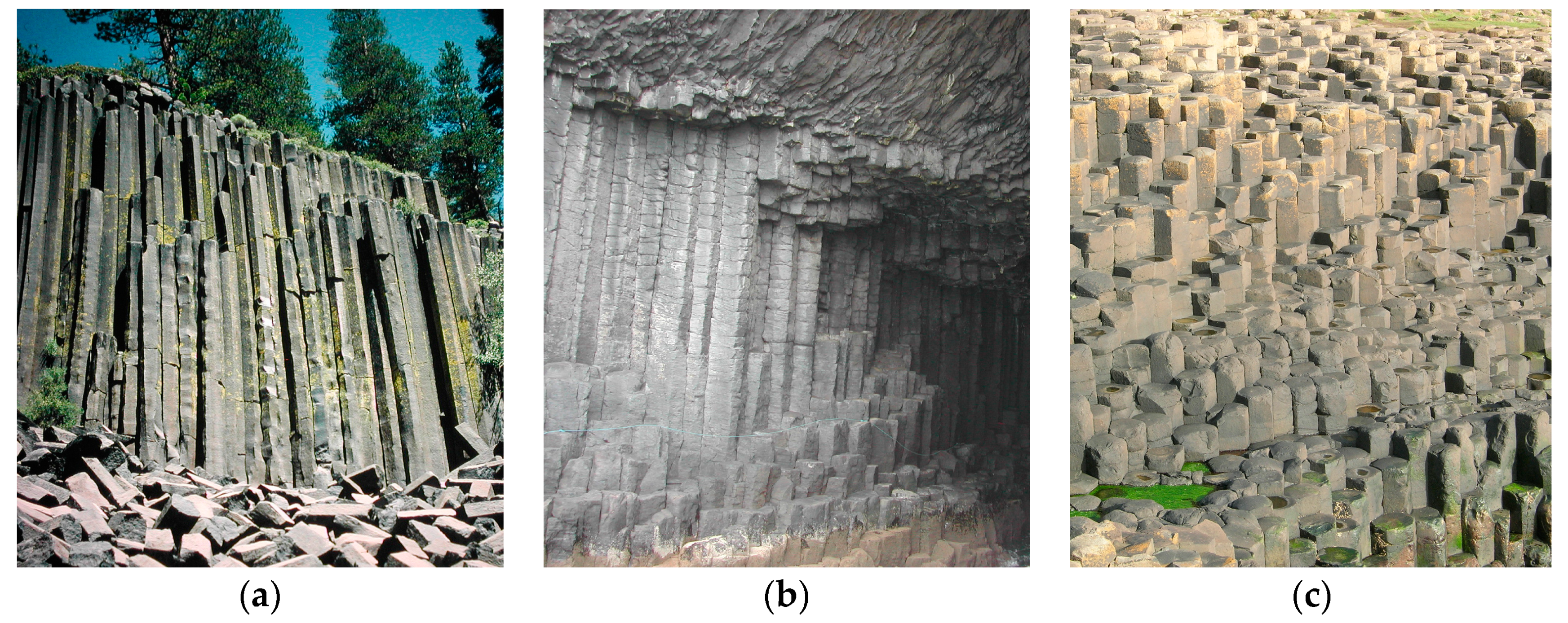
With the development of hydropower station, columnar jointing is often encountered in southwestern China. As a result of cooling lava flows and ash-flow tuffs, it occurs in many types of volcanic rocks in the formation of a regular array of polygonal prisms or columns [21]. Several famous typical columnar joints are shown in Figure 1.
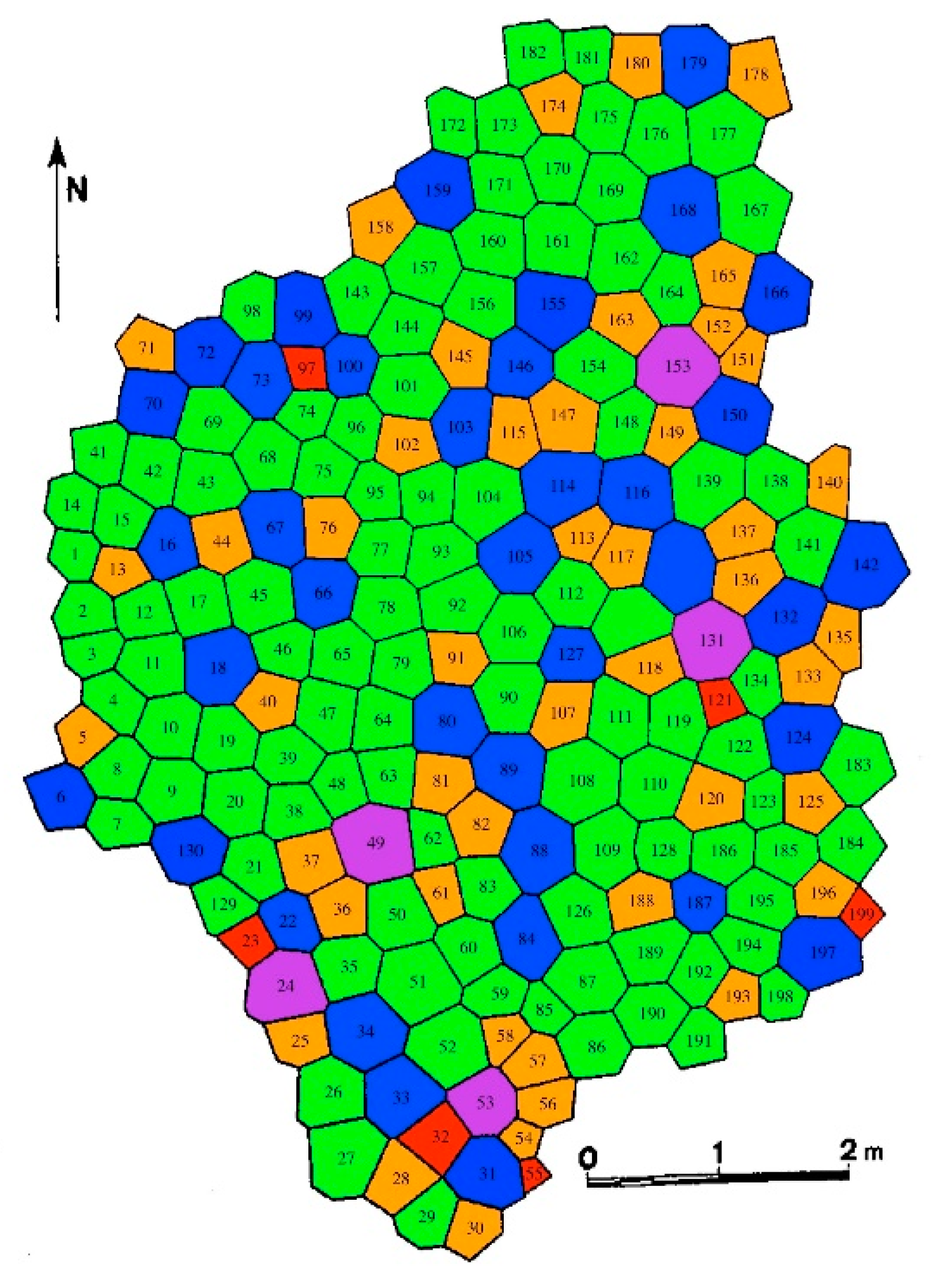
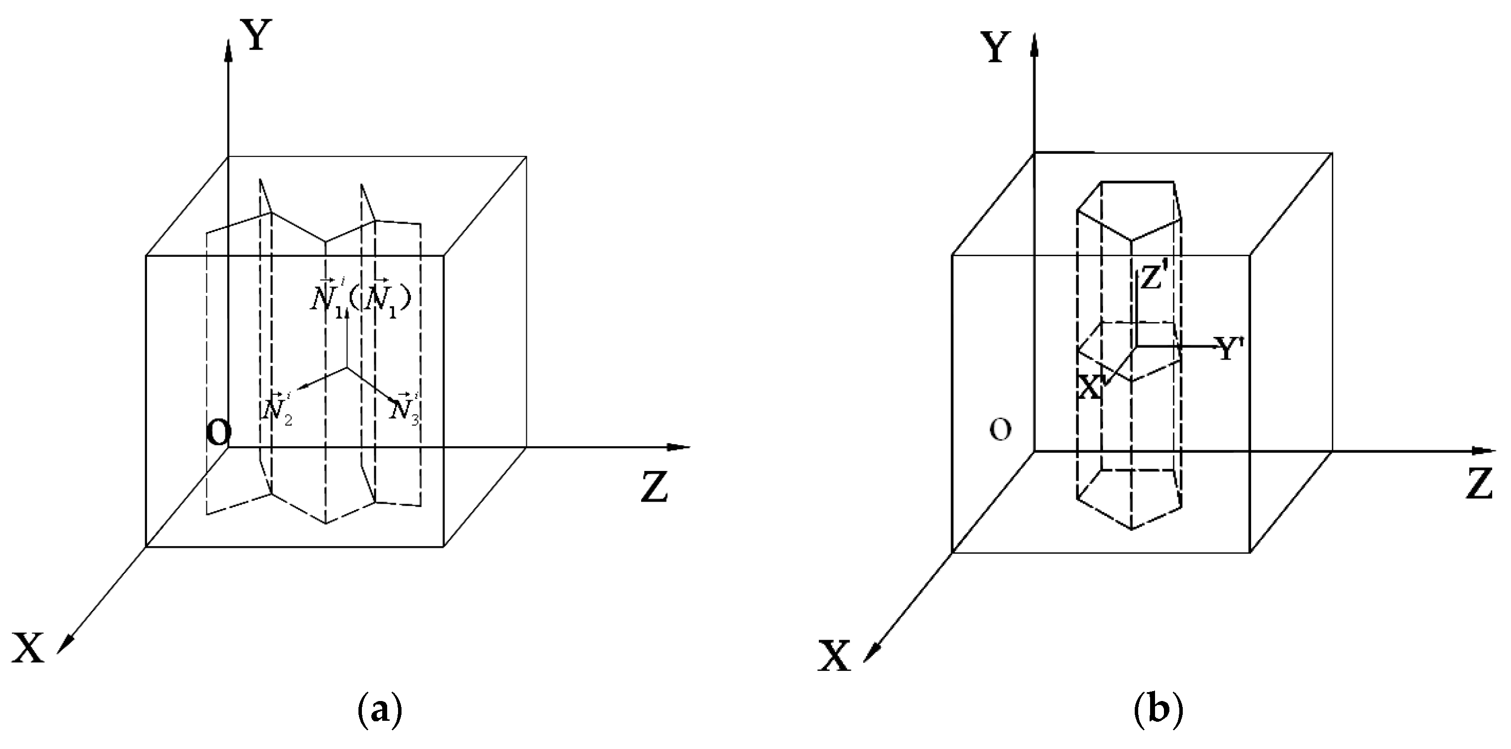
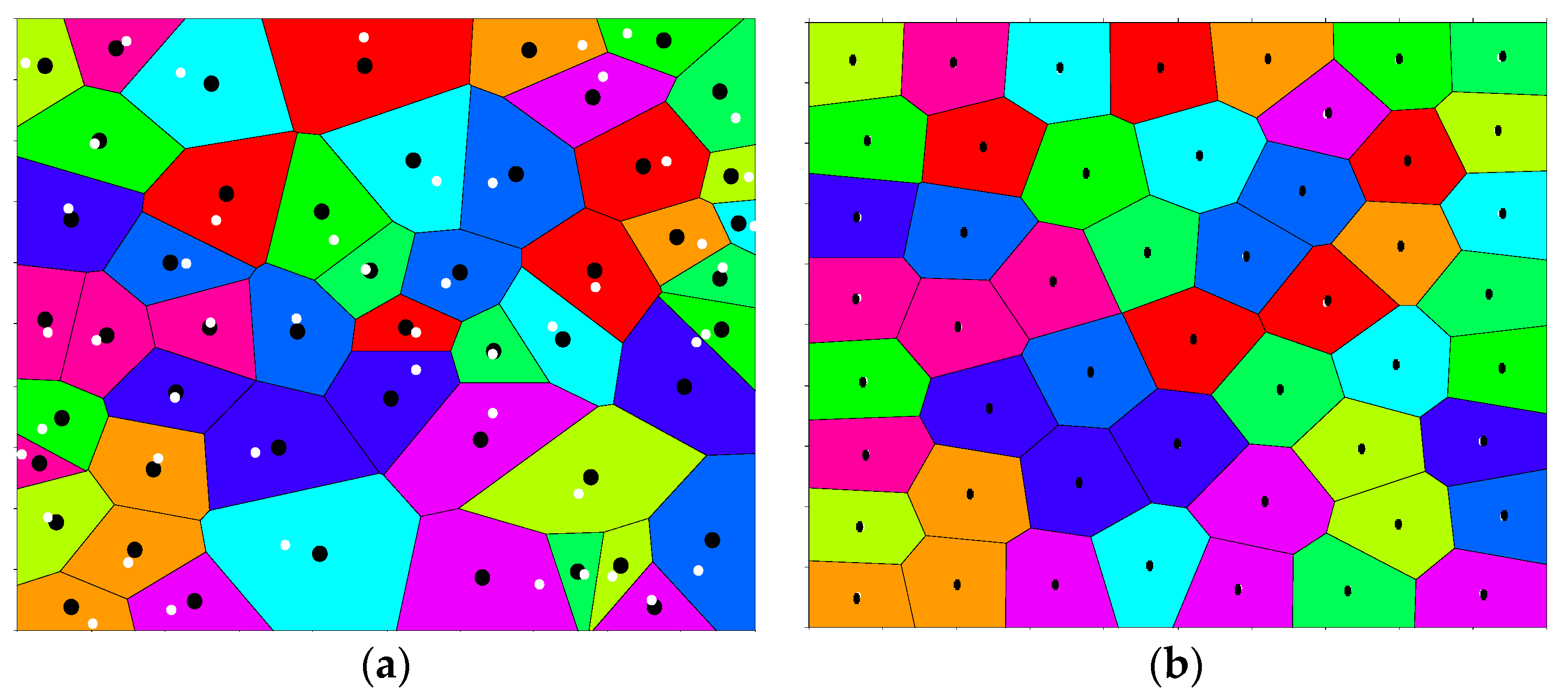
Although the characteristics of columnar jointed rock is typical, they vary for different locations. The column in some areas is regular and straight like Giant’s Causeway, while some other places like Baihetan Dam, it is irregular. Besides, the diameters of columns vary from meters to centimeters. Columns are usually parallel and straight, and the length can be as much as several meters. Furthermore, the number of sides of an individual column also varies from three to eight. In order to give a more specific illustration of the columns, a colorized O’Reilly map is presented in Figure 2. In this figure, hexagons are green, heptagons are blue, octagons are purple, pentagons are orange, and squares are red. From the introduction of columnar jointed rock mass above, a diagrammatic drawing is proposed in Figure 3. It is appropriate to model columnar joints using Voronoi diagrams.
3. Constrained Centroidal Voronoi and Implementation Method
3.1. Voronoi Diagram Algorithm and Its Constraints
3.1.1. Classical Voronoi Tessellation
A Voronoi diagram is a classical domain partitioning method named after Georgy Voronoi, a Russian mathematician. Voronoi generation is the dual algorithm of Delaunay triangulation. A typical Voronoi figure is generated using the perpendicular bisector of the lines composed by a set of points called seeds. The Voronoi diagram is a topic in computational geometry and has already widely applied in some other research areas like hydrology and crystal mechanics.
As shown in Figure 4, a Voronoi diagram with 10 random seeds Pi is generated. It can be seen that the domain is divided into 10 patches and each patch has a single seed. For the generation of a Voronoi diagram, a Delaunay triangulation is first implemented. Then the perpendicular bisector is plotted to partition the domain into different Voronoi cells. With the development of computational geometry, Voronoi tessellation is included in many software and packages like MATLAB, Mathematica, and SciPy. However, there are two obvious shortcomings of the classical Voronoi diagram:
- (a)
- The Voronoi cell is not closed. For the Voronoi diagram in Figure 4, only one cell is closed and the other nine cells are open. This brings inconvenience for the analysis.
- (b)
- The shape of the Voronoi cell is random and it is very hard to generate a Voronoi diagram with a specified statistical distribution.
3.1.2. Constrained Voronoi Diagram Generation
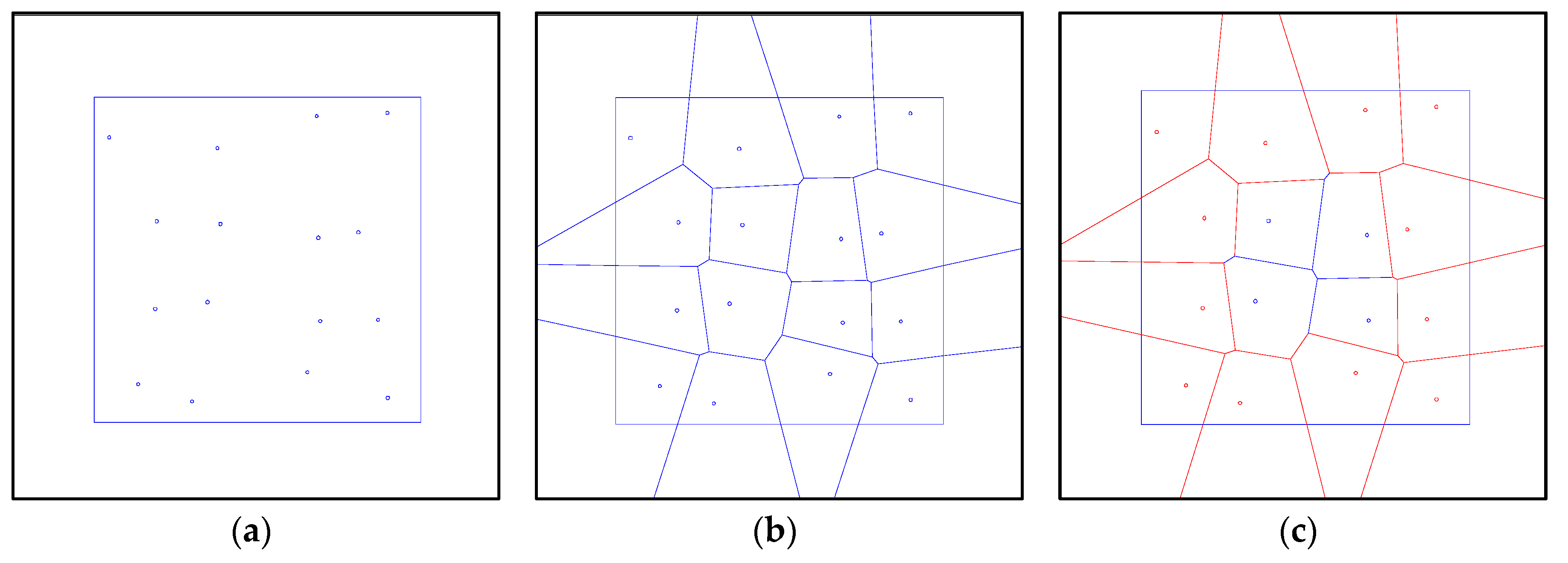
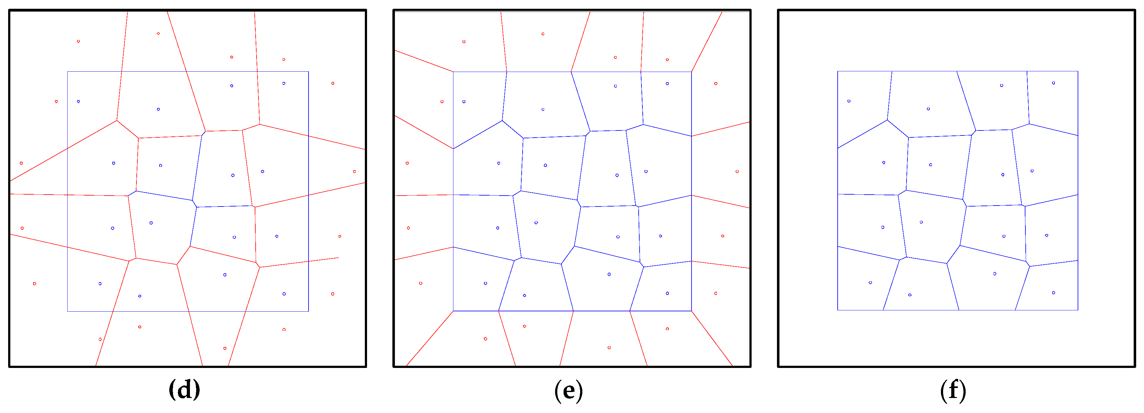
To overcome the first drawback of classical Voronoi tessellation, a constrained Voronoi diagram algorithm is employed to generate a closed Voronoi tessellation with seed points Pi and domain D. Taking a model with 16 points (xi, yi) and a square domain in Figure 5a as example, this algorithm can be described as follows [22]:
- (a)
- A Voronoi diagram is generated using a classical tessellation method (Figure 5b).
- (b)
- All the open cells with a vertex outside the domain D are identified (shown in Figure 5c).
- (c)
- A set of new seeds symmetric to the seeds of open cells with respect to the domain boundary are created (Figure 5d).
- (d)
- New Voronoi diagram is generated with a classical tessellation (Figure 5e).
- (e)
- By removing the open cells as well as the related seeds, the final Voronoi diagram is shown in Figure 5f.
3.2. Centroidal Voronoi Algorithm
3.2.1. Random and Centroidal Voronoi Diagram
The Voronoi diagram created using a constrained Voronoi tessellation method with randomly generated seeds is shown in Figure 6a. It can be seen that the Voronoi cell is irregular and there is a clear deviation between the Voronoi seeds and the centroids. In order to obtain more regular columnar as shown in Figure 2, an algorithm for centroidal Voronoi diagrams (Figure 6b) is proposed to tackle this problem.
Compared with the random Voronoi diagram, the seed of a cell is coincident with its centroid in centroidal Voronoi tessellation (CVT). It is widely used in related fields like mesh generation and data compression. Previous study has indicated that some natural patterns like Giant’s Causeway can be represented by the centroidal Voronoi tessellation [5].
There are a number of methods for the generation of centroidal Voronoi diagram, among which are the algorithms by Lloyd and by MacQueen [23,24], which are widely used, and some other methods are variations of these two methods. Considering that MacQueen’s algorithm needs twice as many Monte Carlo simulations in each iteration, which consumes a large amount computation time, Lloyd’s centroidal method is employed for modelling columnar jointed rock mass in this study.
3.2.2. Lloyd’s Algorithm
In this work, Lloyd’s algorithm, named after Stuart P. Lloyd, is employed. It is an iteration method to partition the domain into well-shaped and uniformly-sized convex cells [25]. The convergence of Lloyd’s algorithm to a centroidal Voronoi diagram has been proven. The random Voronoi diagram can be iterated to a centroidal Voronoi diagram using Lloyd’s algorithm and the algorithm can be simplified as follows:
- (1)
- For an initial seeds yi, generate a Voronoi diagram using constrained Voronoi tessellation;
- (2)
- Compute the centroid zi of the Voronoi diagram of yi;
- (3)
- Move the generating point yi to its centroid zi;
- (4)
- Repeat Steps 1 to 3 until all generating points converge to the centroids.
3.2.3. Estimation of the Centroid
The centroidal Voronoi algorithm is very simple but the calculation of the centroid of each Voronoi cell is time-consuming. In each iteration of Lloyd’s method, the centroidal positions of all shapes of the Voronoi diagram are calculated. Thus, the estimation of the centroid is the most time-consuming task. For determining the centroid of a Voronoi region, a simple formula is:
where χ is the position, Vi is the region area, and ρ(χ) is the density function with ρ(χ) = 1 being the default.
In order to calculate the position of centroid fast, two efficient methods for evaluating the integrals are used in this work. One is based on an integration algorithm on triangle partitions and the other is a sampling method. An integration algorithm can calculate the coordinates of centroids exactly but not as fast as a sampling method; whereas a sampling method is fast but the results are not as accurate as that of an integration algorithm.
(1) Integration method on triangle partitions
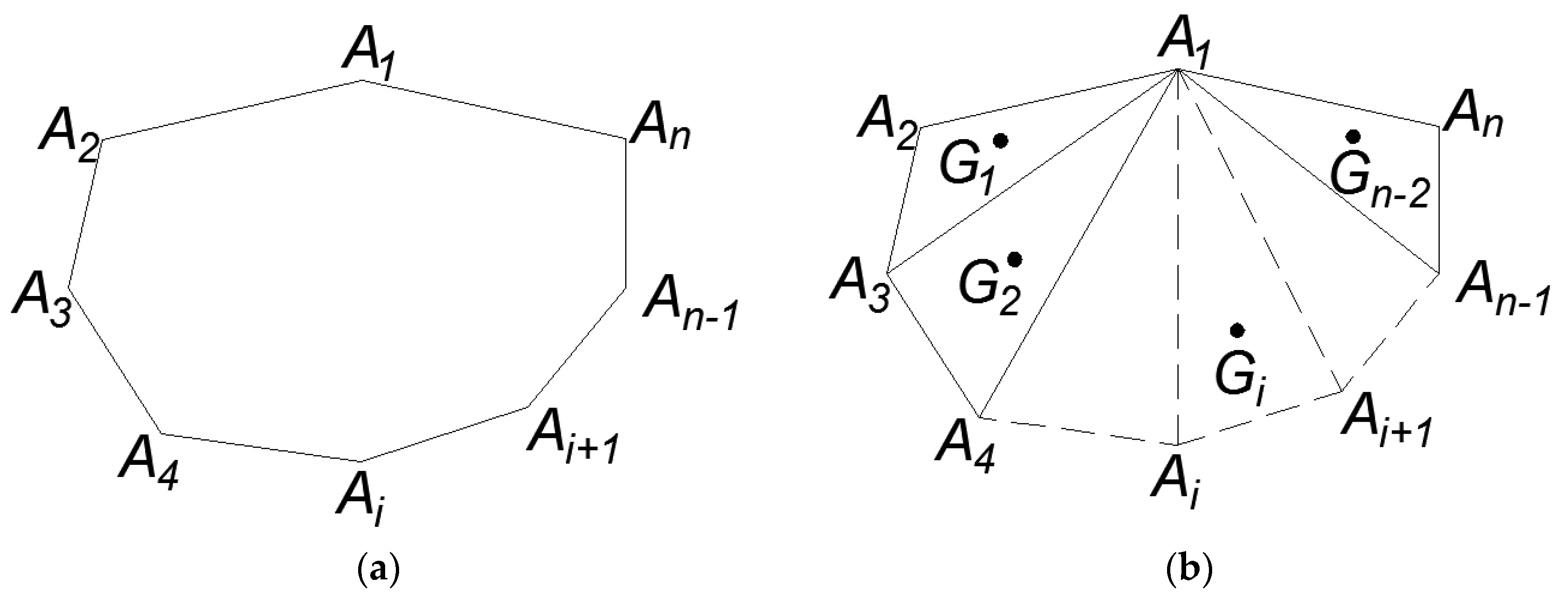
For an arbitrary polygon with n vertices, it can be divided into n − 2 triangles with a clockwise or anti-clockwise direction (Figure 7). For each triangle with vertex Ai (xi, yi) (i = 1, 2, 3), the coordinates of centroid are given by:
The area of the triangle is calculated as:
Considering that the polygon can be discretized into n − 2 triangles and the centroid and area of each triangle can be expressed as Gi(xgi, ygi) and Si, the coordinates of the centroid of the polygon can be obtained as:
(2) Sampling method
Although the integration on triangle partitions is a good solution for the estimation of the centroid of a polygon, it takes a long time to complete each step in Lloyd’s iteration. For a quick calculation, a simple and efficient sampling method is proposed as an alternative.
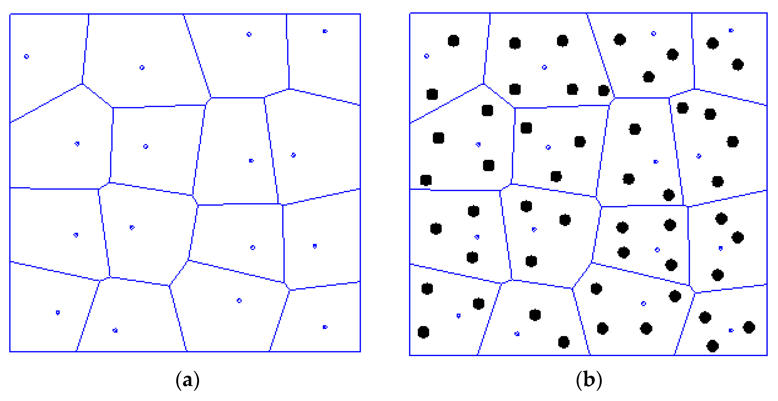
For a certain area with different Voronoi tessellations, a set of random points are distributed in this area (Figure 8). For each Voronoi cell, if there are n points Pi(xi, yi) in this area, then the centroid of this cell can be approximated as the average of these points:
In this way, the determination of centroids changes to the partition of areas into different Voronoi cells, i.e., the “N-D nearest point search” problem. Luckily, the nearest point search problem has a mature mathematical solution [26] and this algorithm has been written in a number of software libraries, such as Python and MATLAB. Using these libraries, all the random points can be divided efficiently and the centroid of Voronoi diagram can be computed quickly. With more sampling points, the calculation of centroid will be more accurate. If the number of random points is selected properly, this algorithm can be both fast and relatively accurate.
3.3. Numerical Implementation and Discussion
In the iterations of Lloyd’s algorithm, the Voronoi generators and centroids are known, and energy can be employed to describe the Voronoi diagram [23]. For the Voronoi tessellation , the energy is defined as:
where is the position of the Voronoi generator, represents the position of the centroid, and is the density function with being the default.
However, if the generator of Voronoi diagram is not known beforehand, energy cannot be estimated. For example, it is not easy to calculate the energy of Voronoi cells in Figure 2. Indirectly, the coefficent of variation, which has been proven as an effective parameter in the estimation of Voronoi diagram [27,28], is employed for the description of the properties of Voronoi cells. In the process of smoothing energy from a randomly-generated Voronoi diagram to a centroidal Voronoi diagram, the coefficient of variation value is recorded with the following formula:
where SD is the standard deviation and m is the mean of Voronoi cell areas. The coefficient of variation gives a quantitative indication on the spatial distribution: the higher the coefficient of variation, the higher the tendency of cells to aggregate into clusters.
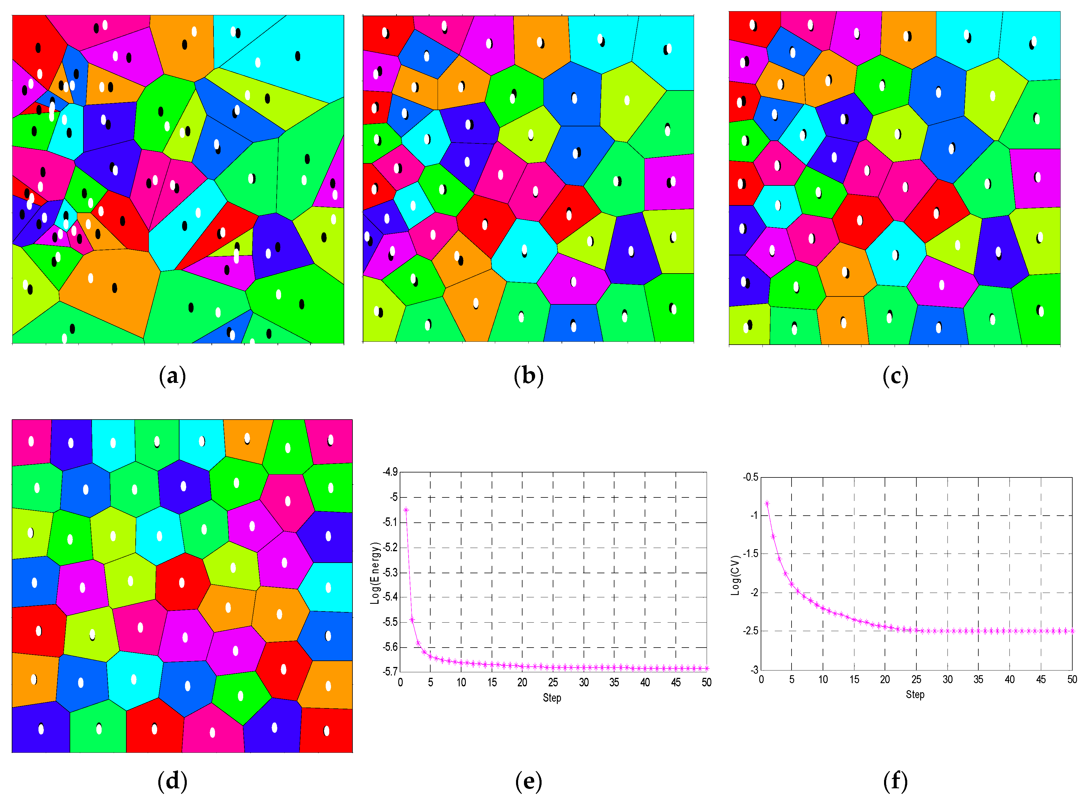
Based on the related algorithms described, numerical implementation is done in MATLAB, in which some good programming techniques from the open-source program of Burkardt are referenced [29]. The 50 seeds for Voronoi diagram are generated randomly. After 50 iterations, the points are well-spaced and Lloyd’s algorithm for computing centroidal Voronoi tessellation converged overall (Figure 9). In this way, the coefficient of variation has the same evolution trend as energy (E), and it is reasonable to use coefficient of variation to describe the distribution property of the Voronoi tessellation.
4. Modeling of Columnar Jointed Rock Mass
Analysis of typical shapes of columnar jointing shows that a columnar jointed rock mass can be modelled through the extrusion of a 2-D Voronoi diagram. Hence, the generation of 2-D columnar jointing, which is consistent with the site condition is a key task. In Section 3, it is shown that coefficient of variation can describe the distribution property in the iterations of Lloyd’s algorithm. The centroidal Voronoi diagram is applicable in the description of a natural phenomenon such as Giant’s Causeway. In fact, natural columnar jointing is not an exactly centroidal Voronoi diagram, and it lies between random and centroidal Voronoi diagrams. In the process of transforming a Voronoi diagram from totally random to centroidal, the value of CV indicates that the Voronoi cells change from heterogeneous to homogeneous. Therefore, it is feasible to describe the characteristics of columnar joints by employing two main parameters: the columnar density representing the scale and coefficient of variation reflecting the variation property.
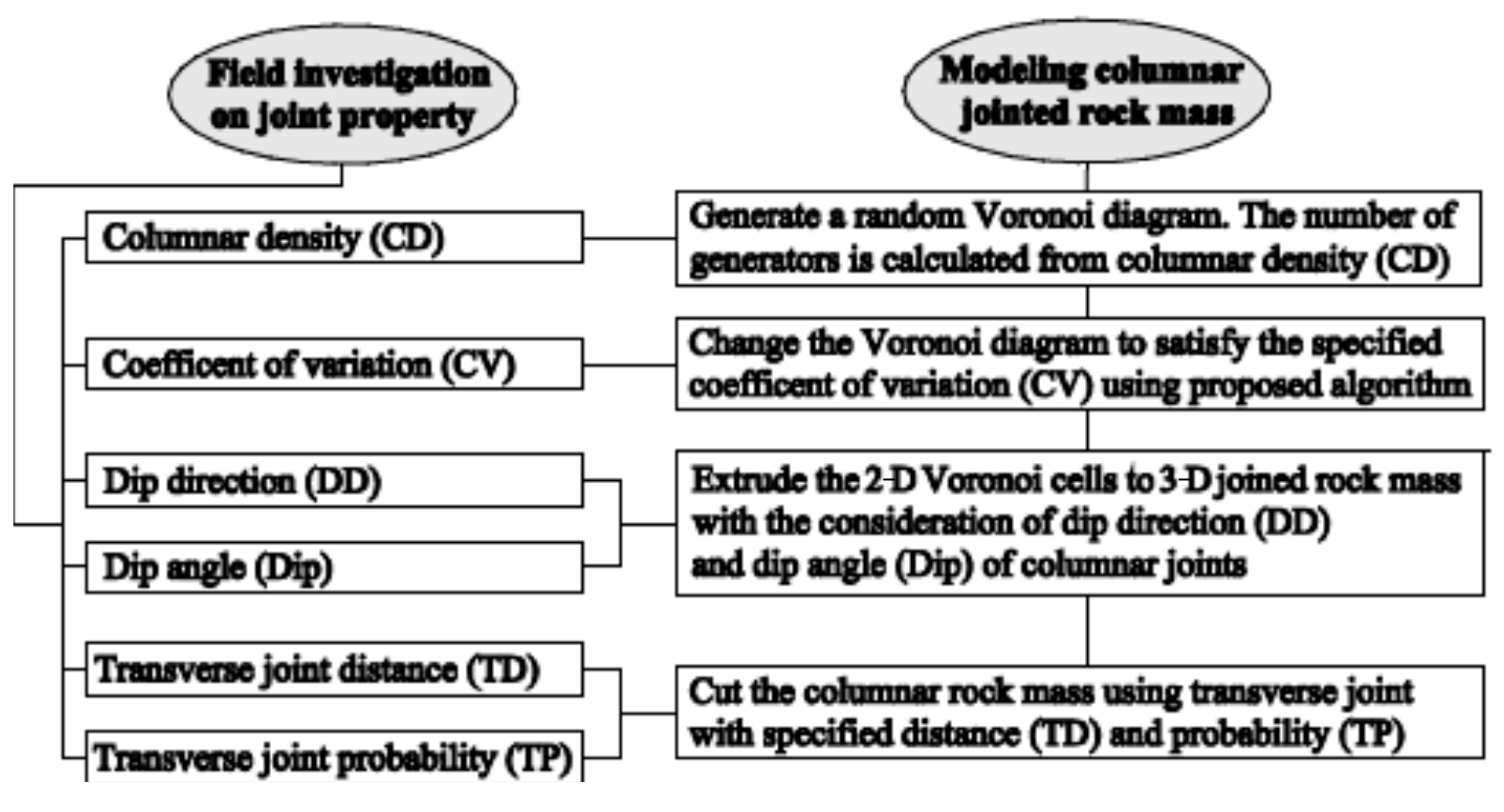
A procedure for the generation of columnar jointed rock mass is proposed (Figure 10). Based on field investigation of geological conditions and site images, the columnar jointing at the site of interest is characterized by six parameters: columnar density (CD), coefficient of variation (CV), dip direction (DD), dip angle (DIP), transverse joint distance (TD), and probability (TP). The number of random seeds for generating a Voronoi diagram is estimated according to the calculated density. Based on the idea of the bisection method, a novel modified constrained centroidal Voronoi smooth algorithm is implemented to make the CV converge to the specified value as follows:
- (1)
- For a Voronoi diagram with CV larger than the specified value, calculate the centroid PC.
- (2)
- The new generator Pnew,g is set at the midpoint of the old generator Pold,g and the centroid PC. Calculate the coefficient of variation CV of the new Voronoi diagram.
- (3)
- Repeat Steps 1 and 2 to obtain the generator until the coefficient of variation CV converges to the specified value with a prescribed accuracy.
Having obtained a 2-D Voronoi diagram with specified CD and CV, it can be extruded to a 3-D columnar shape in accordance with DD and DIP. Then for each extruding Voronoi cell and its length, a transverse joint can be generated by the determination of the intersection between the extruding Voronoi cell and the transverse plane. Sometimes, the transverse joint is non-penetrating, and the transverse joint can be selected with the specified TD and TP. In this way, columnar jointed rock mass with the site properties can be generated.
5. Columnar Joints Generation: A Case Study of the Baihetan Hydropower Station
5.1. Engineering Geological Investigation
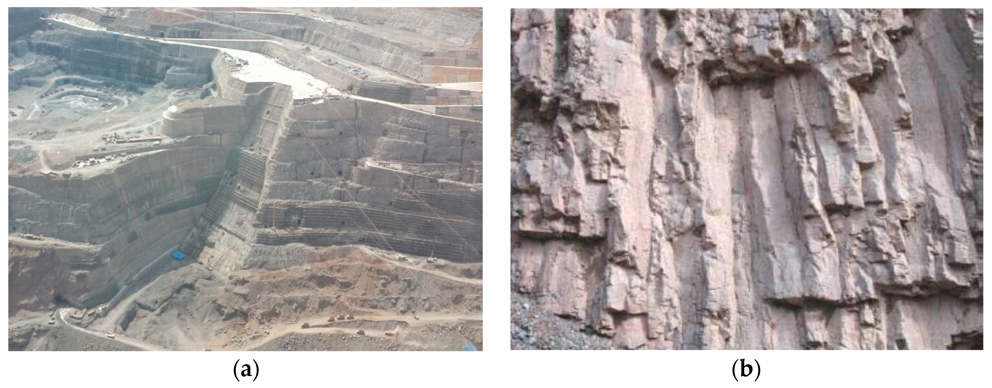
The Baihetan Hydropower Station is a multi-purpose project for harnessing the Yangtze River, developed mainly for power generation, flood control, sediment flushing, and improving the navigation conditions in the reservoir and downstream. The Baihetan Hydropower Station is located on the downstream reaches of the Jinsha River. At the dam site, the most apparent stratigraphic lithology is basalt that belongs to the Emeishan (Emei Mt.) formation of the Permain System (P2β). In the construction of the plant’s hydraulic structures, columnar jointed basalt is found to be widely distributed at the arch dam foundation, underground caverns, abutment slopes, and other water conservancy tunnels (Figure 11).
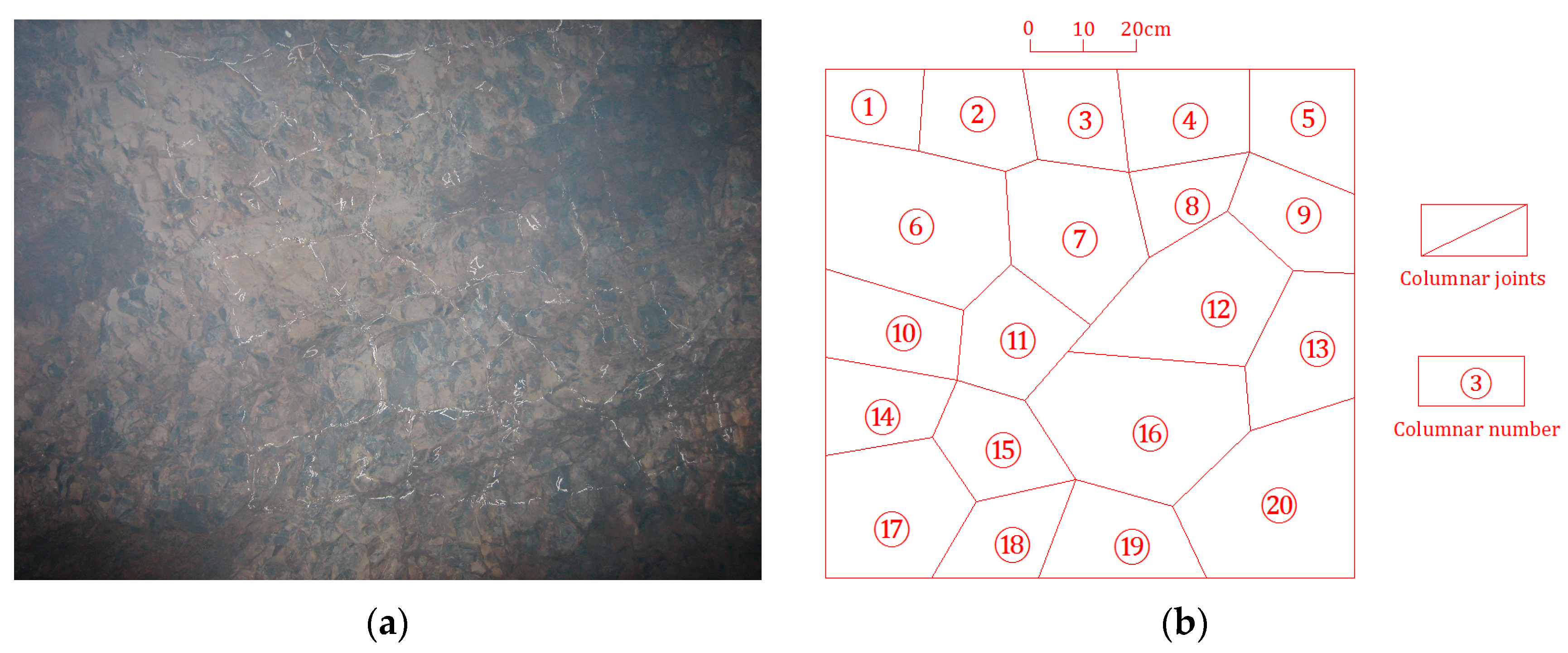
A typical figure of columnar jointed basalt is drawn by the Huadong Engineering Cooperation Limited (ECIDI), as shown in Figure 12 with related parameters listed in Table 1. The orientation of columnar is regular with Dip = 72° and DD = 145°, and the length of columnar is about 1.5 m. Based on the skeleton figure, a digital image processing technique is employed in the analysis. The area of each columnar is calculated and the coefficient of variation is obtained. Using a sample of 10 typical columnar basalt drawings, the statistical mean of coefficient of variation was about 44.18% and it implied that the discreteness of columnar basalt was quite large. Furthermore, the density of columnar cells could also be obtained from skeleton drawings, which gave a density of about 20 in a 1 m × 1 m square.
5.2. Columnar Jointing Model Generation
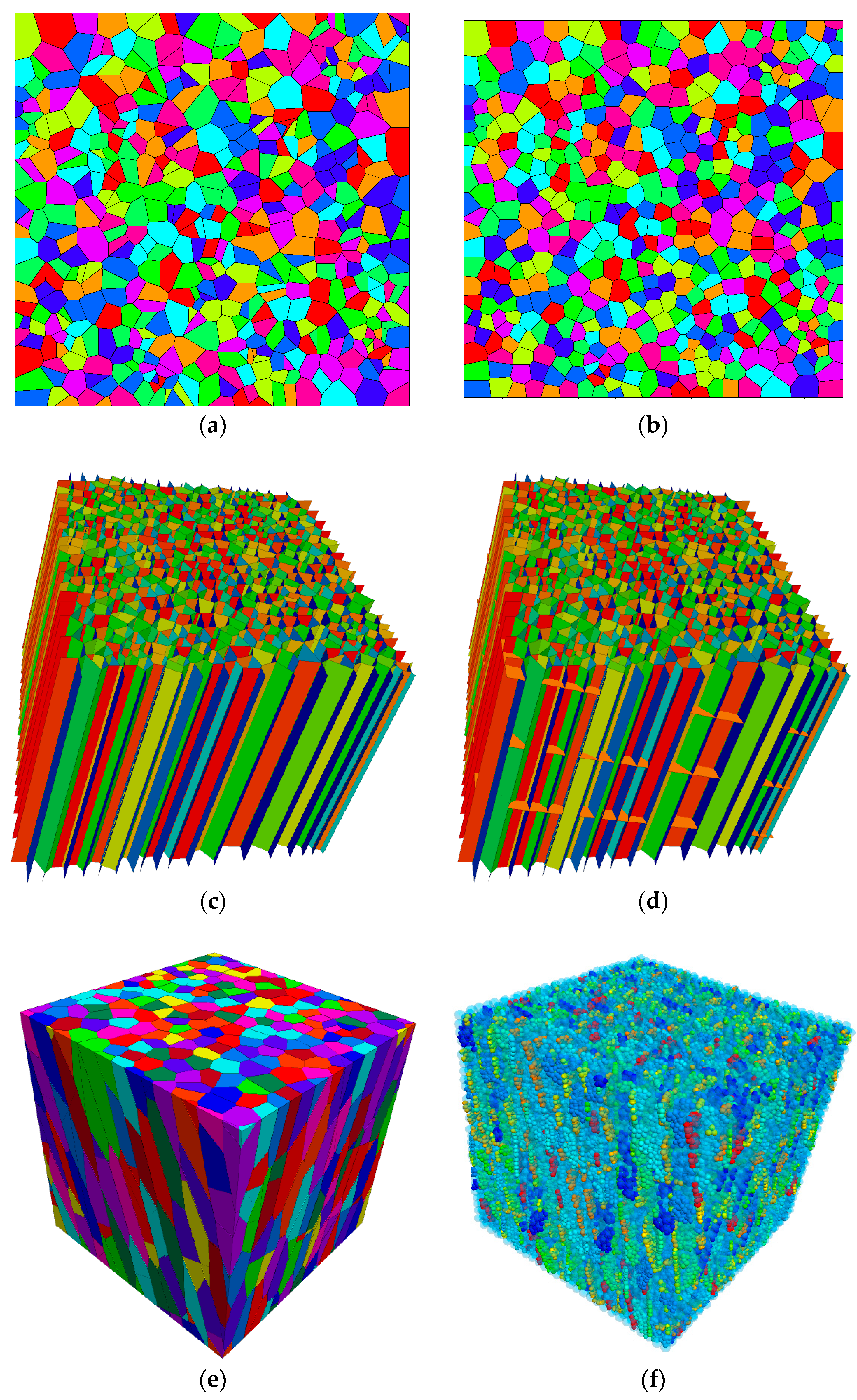
Considering the scale effect of heterogeneous materials, a proper size has to be selected. For convenience, the size of the numerical model was taken as 1 m × 1 m. In order to ensure that the 3-D model could be generated, an initial area of 5 m × 5 m was chosen for the generation of a 2-D Voronoi diagram. From the density of site conditions, it was estimated that about 500 seeds were needed. A random Voronoi diagram was generated in Figure 13a with a CV of 56.45%. With a specified CV value of 44.18%, a Voronoi diagram could be generated (Figure 13b) by applying the algorithm proposed in Section 4. Then an extrusion at a certain direction with parameter DIP and DD was made to extend the rock from 2-D to 3-D (Figure 13c). Afterwards, horizontal hidden joints was implemented to cut the rock (Figure 13d). Using these operations, the coordinates information of all rock blocks could be calculated. By trimming the solid with a certain boundary, the block information of the columnar jointed rock is shown in Figure 13e. It was easier for the particle model in Figure 13f, where the model could be generated by importing the DFN (discrete fracture networks) in Figure 13d to a cubic particle model, which could be done easily in DEM packages like PFC (Particle Flow Code), YADE (Yet another dynamic engine), and LIGGGHTS (LAMMPS improved for general granular and granular heat transfer simulations).
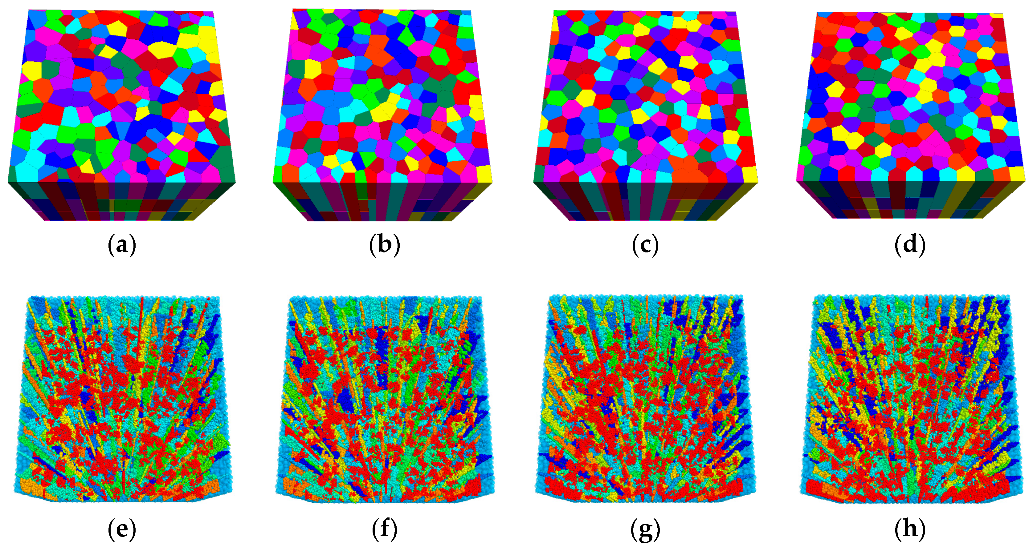
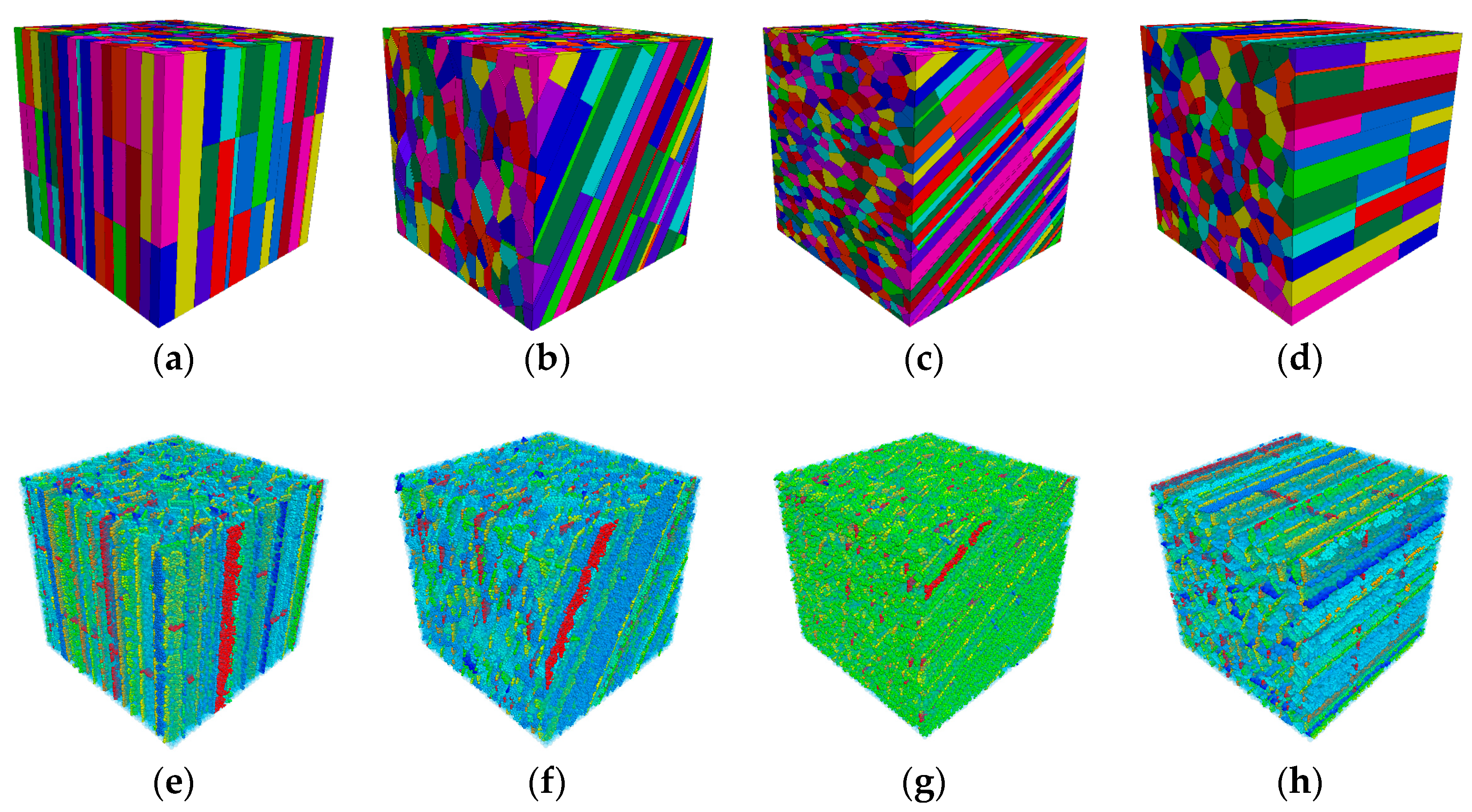
Columnar jointed rock mass with different CV is shown in Figure 14. It can be seen that the volume of columnar became more and more uniform with the decrease of coefficient of variation. Columnar jointed rock masses with different directions are shown in Figure 15. The result shows that the direction was also an important parameter affecting the morphology of columnar jointed rock masses. From all these cases, it can be concluded that this method is applicable and effective in the modeling of columnar jointed rock mass with complex structures, which is extremely helpful in the analysis of physical and mechanical properties of such materials.
6. Conclusions and Discussion
Aimed at the analysis of columnar jointed rock mass with complex structures, this paper proposed a novel method for the generation of numerical model. From the results obtained, the following conclusions can be drawn:
- (1)
- The coefficient of variation is an effective parameter for representing the deviation between the generator and the centroid of Voronoi cell, which has the same effect as energy in a centroidal Voronoi tessellation. Furthermore, it can reflect the heterogeneity of the cells forming the columnar jointed rock mass.
- (2)
- A modified Lloyd’s algorithm is proposed to generate the Voronoi diagram with a specified coefficient of variation. Two algorithms for estimating the centroid were presented and discussed.
- (3)
- This work proposed the description of columnar jointed rock mass with six parameters and a detailed procedure for modelling columnar jointed rock mass. Taking the columnar basalt in the Baihetan hydropower station as an example, numerical models for columnar jointed rock mass with the specified geological properties were generated. The numerical results indicated that the method was effective and efficient.
Author Contributions
Q.M contributed in formulating the research question; Y.C., L.Y. and Q.Z. prepared the original manuscript. All authors contributed in addressing reviewers comments during the review process and proofreading of the accepted manuscript.
Funding
This research was funded by National Key R&D Program of China (2017YFC1501100), the National Natural Science Foundation of China (Grant Nos. 51709089, 11572110, 51479049, 11772116), and Open fund of state key laboratory of hydraulics and mountain river engineering (Sichuan University: SKHL1725) are gratefully acknowledged.
Conflicts of Interest
The authors declare no conflict of interest.
References
- Goehring, L. On the Scaling and Ordering of Columnar Joints; University of Toronto: Toronto, ON, Canada, 2008. [Google Scholar]
- Xu, X.W. Columnar jointing in basalt, Shandong Province, China. J. Struct. Geol. 2010, 32, 1403. [Google Scholar] [CrossRef]
- Bulkeley, R. Part of a Letter from Sir RBSRS to Dr. Lister concerning the Giants Causway in the County of Atrim in Ireland. Philos. Trans. R. Soc. Lond. 1693, 17, 708–710. [Google Scholar]
- Budkewitsch, P.; Robin, P.Y. Modelling the evolution of columnar joints. J. Volcanol. Geotherm. Res. 1994, 59, 219–239. [Google Scholar] [CrossRef]
- DeGraff, J.M.; Long, P.E.; Aydin, A. Use of joint-growth directions and rock textures to infer thermal regimes during solidification of basaltic lava flows. J. Volcanol. Geotherm. Res. 1989, 38, 309–324. [Google Scholar] [CrossRef]
- Ryan, M.P.; Sammis, C.G. Cyclic fracture mechanisms in cooling basalt. Geol. Soc. Am. Bull. 1978, 89, 1295–1308. [Google Scholar] [CrossRef]
- Ryan, M.P.; Sammis, C.G. The glass transition in basalt. J. Geophys. Res. Solid Earth 1981, 86, 9519–9535. [Google Scholar] [CrossRef]
- Müller, G. Experimental simulation of basalt columns. J. Volcanol. Geotherm. Res. 1998, 86, 93–96. [Google Scholar] [CrossRef]
- Müller, G. Experimental simulation of joint morphology. J. Struct. Geol. 2001, 23, 45–49. [Google Scholar] [CrossRef]
- Shorlin, K.A.; de Bruyn, J.R.; Graham, M.; Morris, S.W. Development and geometry of isotropic and directional shrinkage-crack patterns. Phys. Rev. E 2000, 61, 6950. [Google Scholar] [CrossRef]
- Jiang, Q.; Feng, X.T.; Hatzor, Y.H.; Hao, X.J.; Li, S.J. Mechanical anisotropy of columnar jointed basalts: An example from the Baihetan hydropower station, China. Eng. Geol. 2014, 175, 35–45. [Google Scholar] [CrossRef]
- King, M.; Myer, L.; Rezowalli, J. Experimental studies of elastic-wave propagation in a columnar-jointed rock mass. Geophys. Prospect. 1986, 34, 1185–1199. [Google Scholar] [CrossRef]
- Meng, G.T. Geomechanical Analysis of Anisotropic Columnar Jointed Rock Mass and Its Application in Hydropower Engineering; Hohai University: Nanjing, China, 2007. [Google Scholar]
- Zheng, W.T.; Xu, W.Y.; Yan, D.X.; Ji, H. A Three-Dimensional Modeling Method for Irregular Columnar Joints Based on Voronoi Graphics Theory. Applied Informatics and Communication; Springer: Berlin/Heidelberg, Germany, 2011; pp. 62–69. [Google Scholar]
- Di, S.J.; Xu, W.Y.; Ning, Y.; Wang, W.; Wu, G.Y. Macro-mechanical properties of columnar jointed basaltic rock masses. J. Cent. South Univ. Technol. 2011, 18, 2143–2149. [Google Scholar] [CrossRef]
- Shan, Z.G.; Di, S.J. Loading-unloading test analysis of anisotropic columnar jointed basalts. J. Zhejiang Univ. Sci. A 2013, 14, 603–614. [Google Scholar] [CrossRef] [Green Version]
- Yan, D.X.; Xu, W.Y.; Zheng, W.T.; Wang, W.; Shi, A.C.; Wu, G.Y. Mechanical characteristics of columnar jointed rock at dam base of Baihetan hydropower station. J. Cent. South Univ. Technol. 2011, 18, 2157–2162. [Google Scholar] [CrossRef]
- Xu, W.Y.; Zheng, W.T.; Ning, Y.; Meng, G.T.; Wu, G.Y.; Shi, A.C. 3D anisotropic numerical analysis of rock mass with columnar joints for dam foundation. Yantu Lixue 2010, 31, 949–955. [Google Scholar]
- Xiao, W.M.; Deng, R.G.; Zhong, Z.B.; Fu, X.M.; Wang, C.Y. Experimental study on the mechanical properties of simulated columnar jointed rock masses. J. Geophys. Eng. 2015, 12, 80. [Google Scholar] [CrossRef]
- Ning, Y.; Xu, W.Y.; Zheng, W.T. Study of random simulation of columnar jointed rock mass and its representative elementary volume scale. Chin. J. Rock Mech. Eng. 2008, 27, 1202–1208. [Google Scholar]
- O’Reilly, J.P. Explanatory Notes and Discussion of the Nature of the Prismatic Forms of a Group of Columnar Basalts, Giant’s Causeway. (With Plates XV.-XVIII.). Trans. R. Ir. Acad. 1879, 26, 641–734. [Google Scholar]
- Mollon, G.; Zhao, J. Fourier–Voronoi-based generation of realistic samples for discrete modelling of granular materials. Granul. Matter 2012, 14, 621–638. [Google Scholar] [CrossRef]
- Du, Q.; Faber, V.; Gunzburger, M. Centroidal Voronoi Tessellations: Applications and Algorithms. SIAM Rev. 1999, 41, 637–676. [Google Scholar] [CrossRef] [Green Version]
- Du, Q.; Wong, T.W. Numerical studies of MacQueen’s k-means algorithm for computing the centroidal Voronoi tessellations. Comput. Math. Appl. 2002, 44, 511–523. [Google Scholar] [CrossRef]
- Lloyd, S.P. Least squares quantization in PCM. IEEE Trans. Inf. Theory 1982, 28, 129–137. [Google Scholar] [CrossRef] [Green Version]
- Barber, C.B.; Dobkin, D.P.; Huhdanpaa, H. The quickhull algorithm for convex hulls. ACM Trans. Math. Softw. 1996, 22, 469–483. [Google Scholar] [CrossRef]
- Duyckaerts, C.; Godefroy, G. Voronoi tessellation to study the numerical density and the spatial distribution of neurones. J. Chem. Neuroanat. 2000, 20, 83–92. [Google Scholar] [CrossRef]
- Minciacchi, D.; Granato, A. How relevant are subcortical maps for the cortical machinery? An hypothesis based on parametric study of extra-relay afferents to primary sensory areas. Adv. Psychol. 1997, 119, 149–168. [Google Scholar]
- Burkardt, J. 2015. Available online: http://people.sc.fsu.edu/~jburkardt/m_src/cvt_2d_sampling/cvt_2d_sampling.html (accessed on 21 October 2018).
Figure 1.
Typical columnar jointed rock masses: (a) Devil’s Postpile, Yosemite in California; (b) Fingal’s Cave, Staffa in Scotland; and (c) Giant’s Causeway, Antrim in Northern Ireland.
Figure 1.
Typical columnar jointed rock masses: (a) Devil’s Postpile, Yosemite in California; (b) Fingal’s Cave, Staffa in Scotland; and (c) Giant’s Causeway, Antrim in Northern Ireland.

Figure 2.
A colorized map of about 200 columns at the Giant’s Causeway made by O’Reilly in 1879 [1,21].

Figure 3.
Diagrammatic drawing of the joints in columnar basalt: (a) vertical columnar joint, and (b) horizontal transverse joint.
Figure 3.
Diagrammatic drawing of the joints in columnar basalt: (a) vertical columnar joint, and (b) horizontal transverse joint.

Figure 4.
An illustration of Voronoi tessellation with 10 generators: (a) a set of generators, and (b) the resulting Voronoi diagram.
Figure 4.
An illustration of Voronoi tessellation with 10 generators: (a) a set of generators, and (b) the resulting Voronoi diagram.

Figure 5.
Illustration of the stages of the constrained Voronoi tessellation algorithm: (a) initial seeds, (b) classical Voronoi tessellation, (c) open Voronoi cells, (d) symmetry seeds, (e) new Voronoi tessellation, (f) constrained Voronoi diagram.
Figure 5.
Illustration of the stages of the constrained Voronoi tessellation algorithm: (a) initial seeds, (b) classical Voronoi tessellation, (c) open Voronoi cells, (d) symmetry seeds, (e) new Voronoi tessellation, (f) constrained Voronoi diagram.


Figure 6.
Random and centroidal Voronoi diagram: generators (white dots) and centroids (black dots): (a) random Voronoi diagram, and (b) centroidal Voronoi diagram.
Figure 6.
Random and centroidal Voronoi diagram: generators (white dots) and centroids (black dots): (a) random Voronoi diagram, and (b) centroidal Voronoi diagram.

Figure 7.
Discretization of n-polygon: (a) polygon with n vertices, and (b) n − 2 discrete triangles.
Figure 7.
Discretization of n-polygon: (a) polygon with n vertices, and (b) n − 2 discrete triangles.

Figure 8.
Illustration of the sampling method: (a) Voronoi tessellation, and (b) random sampling points.
Figure 8.
Illustration of the sampling method: (a) Voronoi tessellation, and (b) random sampling points.

Figure 9.
Implementation of the constrained centroidal Voronoi algorithm: (a) initial condition, (b) step 5, (c) step 20, (d) step 50, (e) change of energy, and (f) change of coefficient of variation.
Figure 9.
Implementation of the constrained centroidal Voronoi algorithm: (a) initial condition, (b) step 5, (c) step 20, (d) step 50, (e) change of energy, and (f) change of coefficient of variation.

Figure 10.
Procedure for modelling columnar joints.

Figure 11.
Site conditions of the Baihetan Hydropower Station: (a) construction site, and (b) typical columnar jointed basalt.
Figure 11.
Site conditions of the Baihetan Hydropower Station: (a) construction site, and (b) typical columnar jointed basalt.

Figure 12.
Typical P2β3 columnar basalt at Baihetan Hydropower Station: (a) geological photo, and (b) joints skeleton.
Figure 12.
Typical P2β3 columnar basalt at Baihetan Hydropower Station: (a) geological photo, and (b) joints skeleton.

Figure 13.
Numerical specimen generation: (a) Voronoi diagram with CV = 56.45%, (b) Voronoi diagram with CV = 44.18%, (c) extrude 2-D Voronoi diagram with direction, (d) cut columnar rock with transverse joint, (e) block model of columnar rock, and (f) particle model of columnar rock.
Figure 13.
Numerical specimen generation: (a) Voronoi diagram with CV = 56.45%, (b) Voronoi diagram with CV = 44.18%, (c) extrude 2-D Voronoi diagram with direction, (d) cut columnar rock with transverse joint, (e) block model of columnar rock, and (f) particle model of columnar rock.

Figure 14.
Columnar joints with different coefficient of variation: (a) block model with CV = 40%, (b) block model with CV = 30%, (c) block model with CV = 20%, (d) block model with C = 10%, (e) particle model with CV = 40%, (f) particle model with CV = 30%, (g) particle model with CV = 20%, and (h) particle model with CV = 10%.

Figure 15.
Columnar joints with different joint dip angles: (a) block model with dip = 0°, (b) block model with dip = 30°, (c) block model with dip = 60°, (d) block model with dip = 90°, (e) particle model with dip = 0°, (f) particle model with dip = 30°, (g) particle model with dip = 60°, and (h) particle model with dip = 90°.


Table 1.
Parameters of columnar jointed rock mass in dam foundation of Baihetan Hydropower Station.
| Parameter | Dip | DD | CD | CV | TD | TP |
|---|---|---|---|---|---|---|
| Values | 72° | 145° | 25/m2 | 44.18% | 1.5 m | 0.3 |
© 2018 by the authors. Licensee MDPI, Basel, Switzerland. This article is an open access article distributed under the terms and conditions of the Creative Commons Attribution (CC BY) license (http://creativecommons.org/licenses/by/4.0/).
Share and Cite
MDPI and ACS Style
Meng, Q.; Yan, L.; Chen, Y.; Zhang, Q. Generation of Numerical Models of Anisotropic Columnar Jointed Rock Mass Using Modified Centroidal Voronoi Diagrams. Symmetry 2018, 10, 618. https://doi.org/10.3390/sym10110618
AMA Style
Meng Q, Yan L, Chen Y, Zhang Q. Generation of Numerical Models of Anisotropic Columnar Jointed Rock Mass Using Modified Centroidal Voronoi Diagrams. Symmetry. 2018; 10(11):618. https://doi.org/10.3390/sym10110618
Chicago/Turabian StyleMeng, Qingxiang, Long Yan, Yulong Chen, and Qiang Zhang. 2018. "Generation of Numerical Models of Anisotropic Columnar Jointed Rock Mass Using Modified Centroidal Voronoi Diagrams" Symmetry 10, no. 11: 618. https://doi.org/10.3390/sym10110618
Note that from the first issue of 2016, this journal uses article numbers instead of page numbers. See further details here.