Article

Accuracy and Precision of Habitat Structural Complexity Metrics Derived from Underwater Photogrammetry

1
School of Biological Sciences, University of Sydney, Sydney, NSW 2006, Australia
2
Sydney Institute of Marine Science, 19 Chowder Bay Road, Mosman, NSW 2088, Australia
*
Author to whom correspondence should be addressed.
These authors contributed equally to this work.
Remote Sens. 2015, 7(12), 16883-16900; https://doi.org/10.3390/rs71215859
Submission received: 20 September 2015 / Revised: 27 November 2015 / Accepted: 7 December 2015 / Published: 15 December 2015
(This article belongs to the Special Issue Remote Sensing for Coral Reef Monitoring)

Abstract

:
In tropical reef ecosystems corals are the key habitat builders providing most ecosystem structure, which influences coral reef biodiversity and resilience. Remote sensing applications have progressed significantly and photogrammetry together with application of structure from motion software is emerging as a leading technique to create three-dimensional (3D) models of corals and reefs from which biophysical properties of structural complexity can be quantified. This enables the addressing of a range of important marine research questions, such as what the role of habitat complexity is in driving key ecological processes (i.e., foraging). Yet, it is essential to assess the accuracy and precision of photogrammetric measurements to support their application in mapping, monitoring and quantifying coral reef form and structure. This study evaluated the precision (by repeated modeling) and accuracy (by comparison with laser reference models) of geometry and structural complexity metrics derived from photogrammetric 3D models of marine benthic habitat at two ecologically relevant spatial extents; individual coral colonies of a range of common morphologies and patches of reef area of 100s of square metres. Surface rugosity measurements were generally precise across all morphologies and spatial extents with average differences in the geometry of replicate models of 1–6 mm for coral colonies and 25 mm for the reef area. Precision decreased with complexity of the coral morphology, with metrics for small massive corals being the most precise (1% coefficient of variation (CV) in surface rugosity) and metrics for bottlebrush corals being the least precise (10% CV in surface rugosity). There was no indication however that precision was related to complexity for the patch-scale modelling. The 3D geometry of coral models differed by only 1–3 mm from laser reference models. However, high spatial variation in these differences around the model led to a consistent underestimation of surface rugosity values for all morphs of between 8% and 37%. This study highlights the utility of several off-the-shelf photogrammetry tools for the measurement of structural complexity across a range of scales relevant to ecologist and managers. It also provides important information on the accuracy and precision of these systems which should allow for their targeted use by non-experts in computer vision within these contexts.

Graphical Abstract

1. Introduction and Background

Structural complexity plays an important role in structuring biotic assemblages and in maintaining biodiversity of benthic marine ecosystems [1]. The structure of intertidal and subtidal rocky reefs has been shown to be a major factor in the dynamics of resident organisms [2,3,4]. Biogenic habitats provided by organisms such as oysters, mangroves, seagrass, macroalgae, and corals are critical to the integrity of their resident assemblages ([1] and references therein). This is well studied in coral reef habitats where complexity is strongly related to important aspects of ecosystem function and service including coral cover, grazing pressure, fish density and biomass, and even tourism and shoreline protection [5,6,7].
As marine ecosystems are threatened from many anthropogenic and natural forces, there has been an increasing focus on not only understanding the linkages between complexity and function but on the more basic issue of how to measure it accurately and over scales relevant to both ecological processes driving ecosystem trajectories and management [5]. This issue is of particular concern in coral reef ecosystems where the threats to biodiversity are derived from the loss of structural complexity due to the interactive effects of stressors such as coral bleaching, overfishing, cyclones, coastal development, and outbreaks of predator species [8,9].
Structural complexity has been estimated over a range of spatial extents from individual coral heads to 100s of kms using a variety of tools. At very large spatial extents, variables such as bottom roughness and slope have been derived from airborne Lidar [10,11] and sub-surface acoustic profiling [12,13,14,15]. Over smaller areas the direct measurement of factors such as vertical relief, number of holes, surface roughness, and even fractal dimension [5,16,17,18] have been commonly estimated by divers. Among these techniques there has always been a tradeoff between area covered and resolution obtained such that very precise and accurate methodologies were often only practical over very small areas. However, recent advances in image processing algorithms and computing power has seen a proliferation of techniques to estimate structural complexity for large reef areas based on digital photogrammetry and application of structure from motion software [16,19,20,21,22,23].
Photogrammetry was originally used to measure the structural complexity of marine biological targets in intertidal habitats by Beck [24]. This method soon caught on and was used to measure the structural complexity of corals and other marine organisms [25]. Photogrammetry involves the reconstruction of a real-scale three-dimensional (3D) model of a given object or scenario from a series of overlapping photographs, taken from multiple perspectives. This method only requires a consumer-grade digital camera and basic training to ensure overlap of photos [22]. 3D reconstruction is facilitated by an increasing number of software packages, some of them freely available and open source. Enabling non-destructive, repeatable measurements of shape, volume, and surface area, photogrammetry provides a permanent record of the 3D coral and allows it to be monitored over time, with visualisation and measurement of any change in structural complexity. The rapid speed of sampling enables the study of corals in remote reefs or deep slopes, which may have previously been intractable to study [26].
Underwater photogrammetry has proven to be a relatively accurate technique for morphological measurements of hemispherical scleractinian corals with studies demonstrating mean differences in 3D surface areas of 0.85% [25], <5% [27], 13% [26], and 1%–17% [28] and differences in volume of 1.7% [26], 3% [29], to 5%–9% [28]. Accuracy does seem to decrease for more complex branching and disc growth forms with errors in volume of 8% [28] and 17%–24% [29] and in surface area of 2% [28] and 12%–78% [27]. Comparisons of model geometry accuracy are less common although McKinnon et al. [30] demonstrated that photogrammetry can produce models of corals which are >90% similar to those of reference models derived from laser scans.
While studies which look at small-scale complexity (e.g., individual coral colonies), are generating photogrammetric tools to replace more conventional and destructive methods for estimating important characteristics such as surface area and volume, there is now increasing interest in applying these tools over larger spatial extents. Systems have been developed to successfully map and model large areas of benthic habitat (up to ~500 m2) [19,31,32] or even km long transects [23] with a variety of off-the-shelf to custom-built hardware and software packages. Photogrammetry-based models derived from these various processes have been used to look at the relative benefits of various metrics of structural complexity used to characterise benthic habitats [16,20].
The detailed understanding of habitat complexity over a range of scales that can be delivered by photogrammetry tools has the potential to vastly improve our ability to understand, monitor, and manage benthic marine habitats. For instance, these tools could be used on coral reefs to map and monitor the effects of bleaching, cyclone damage, or even outbreaks of crown of thorns starfish on structural complexity. This motivation is driving a rapidly expanding use of techniques to estimate complexity, especially photogrammetry. However the long-term utility of these methods depends very much on the accuracy and precision with which the tools can estimate structural complexity. While the accuracy of conventional metrics like volume and surface area have been well considered at small (coral colony) spatial extents (as outlined above), there has been little work comparing either the geometry (3D structure) of derived models with those of highly accurate references (but see [30]) or any derived metrics of structural complexity. Aside from limited work using reference models [28] there has also been little assessment of the precision (repeatability) of photogrammetry approaches at small scales (but see [29]). At spatial extents larger than an individual coral colony it becomes quite difficult to have any true reference model against which to compare those generated from photogrammetry approaches. Thus, accuracy is nearly impossible to assess. There is also a dearth of information on the precision of such models of benthic habitat and derived structural complexity metrics at these larger spatial extents. This gap in knowledge is especially important to address as this is the very information needed to inform questions as to the level of physical change (mm-cm?) in structural complexity that is actually possible to detect with these systems and thus their potential application for monitoring and threat assessment.
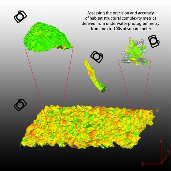
In this study we conducted an assessment of the error (precision and accuracy) involved in mapping marine benthic habitat features at two spatial extents: (1) the coral colony level and (2) the reef patch (100 m2) level. These two levels are quite relevant to the use of structural complexity data in management and ecological studies as they represent spatial extents used to ask questions about reef growth and erosion (colony scale) and relationships between structural complexity and resident assemblages (patch scale) where assemblages are typically assessed using survey areas of this size. We used readily available and thus commonly employed photogrammetric tools—hardware and software. At the colony extent level we imaged coral colonies representing six of the most common coral morphotypes on coral reefs. We quantified precision by repeatedly imaging and modeling individual colonies multiple times. For four of the morphotypes we quantified accuracy by comparing models derived from photogrammetry with those produced by high resolution laser scanning. At the patch extent we adopted a similar approach and repeatedly imaged and modeled an area of rocky reef of surface rugosity (defined below) similar to a coral reef flat. We focused our comparisons to determine the error in the 3D geometry of the models and in the derived surface rugosity metric. Both of these help specify the ability of the photogrammetry techniques used to detect change in complexity on reefs over time. We assessed the limitations of the systems used and the types of ecological questions that can and cannot be addressed with these systems. This information is critical if these novel techniques are to play a major role in either the monitoring of changes in structural complexity or simply its measurement in order to further understand its seemingly critical role as a predictor of the distribution and abundance of organisms in marine systems.

2. Data and Methodology

This study evaluated the precision and accuracy of habitat structural complexity metrics derived from high resolution photogrammetric models (mesh resolutions of 1 to 30 mm, depending on the spatial extent) of benthic marine habitats at two spatial extents; sub-meter (coral colonies) and 100s of meters (patches of benthic habitat). All tools used (hardware and software) are off-the shelf (in some cases free) components that can be used by non-experts in computer vision to suit the specific application. Precision was assessed by sampling the same coral or habitat patch multiple times to evaluate the among-sample variation (measurement error). Accuracy was assessed by comparing metrics and 3D geometry of models generated from photogrammetry with those obtained from laser-scanning (0.2 mm mesh resolution, details below). Accuracy assessment was only possible at the colony-scale. By necessity, the data acquisition and processing methodology for these two spatial scales was different as detailed below. The process flow is summarized in
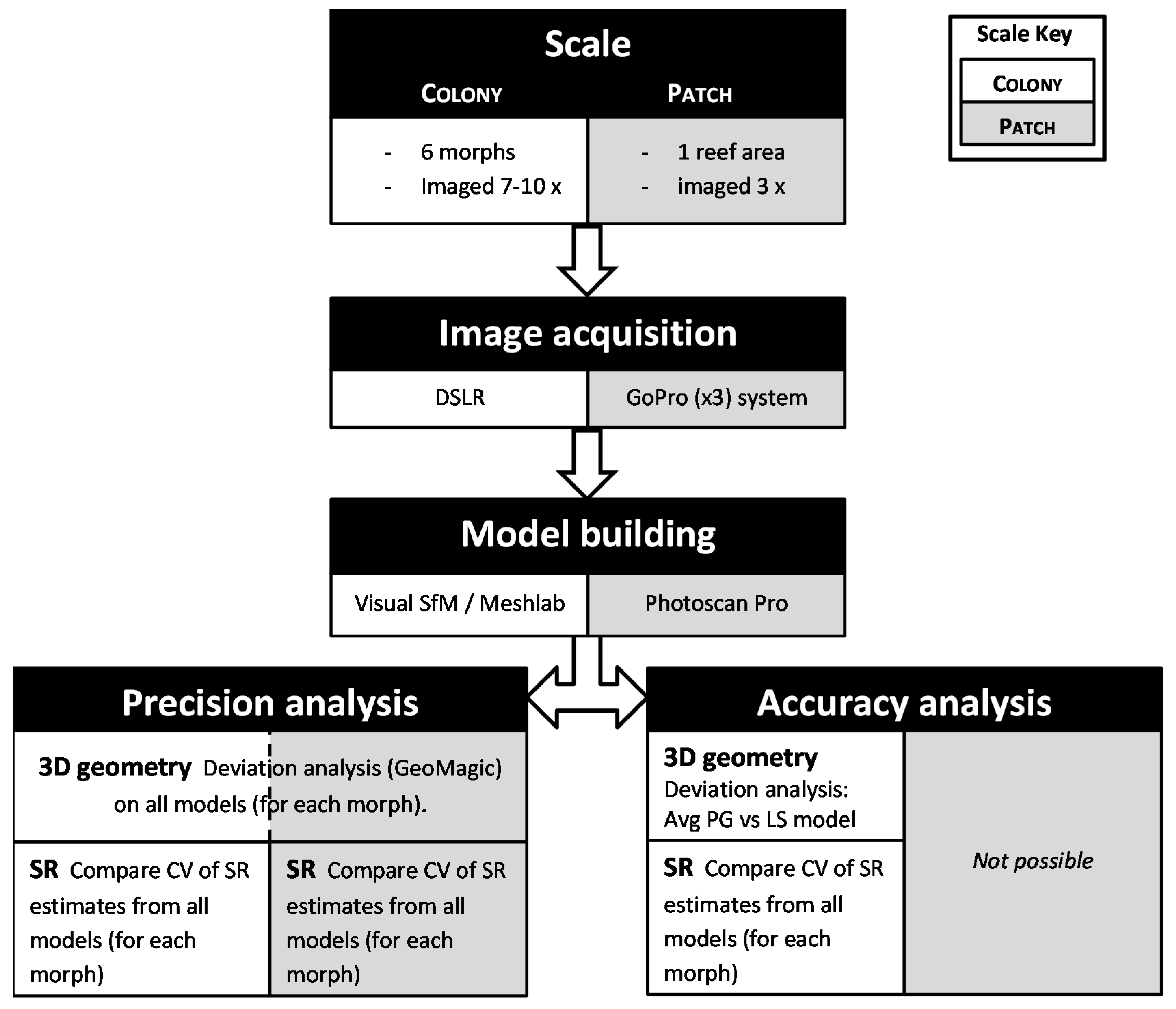
 Figure 1.
Figure 1. Flow diagram of project methodology indicating the systems used to acquire images, build models and conduct precision and accuracy analysis for each of the two spatial scales, colony and reef patch. SR = surface rugosity, PG = photogrammetry and LS = laser scan. For detailed methodology of individual steps see text.
Remotesensing 07 15859 g001

2.1. Subjects and Image Acquisition

2.1.1. Colony-Scale

The subjects for the small-scale assessments were individual coral colonies. In order to allow for unobstructed views of the coral without the need to physically damage them by moving them in the field, we worked with specimens of whole coral colonies representing the major morphotypes loaned from the Australian Museum. Up to 10 individual coral colonies ranging in size from 15–50 cm diameter of six different morphologies were used in the small-scale study; (1) small-sized massive (~12 cm diameter); (2) medium-sized massive (with crevices, ~30 cm diameter); (3) tabulate; (4) coarse branching; (5) foliose; and (6) bottlebrush. As the thin layer of tissue on living corals only contributes a small percentage to their complexity [33], use of the coral skeleton allowed us to document biologically relevant levels of complexity.
Image acquisition for each coral colony was conducted by snorkel in a pool at a depth of 1.2 m, which offered similar conditions to those of a shallow coral reef lagoon for underwater photogrammetry, with natural light variation (i.e., light rays filtering and reflecting on bottom), passing swimmers in the near background (i.e., passing fish), and clear water (although sea water can be slightly more turbid than fresh water; Figure 2). Images were taken using a 24 MP Sony NEX-7 digital camera, with a fixed Sony 16 mm f/2.8 E-mount wide-angle lens to reduce spherical distortion. The camera was in a waterproof Nauticam housing with a dome port. A dome port was chosen over a flat port in order to eliminate refraction and loss of image quality along the edges of the frame.
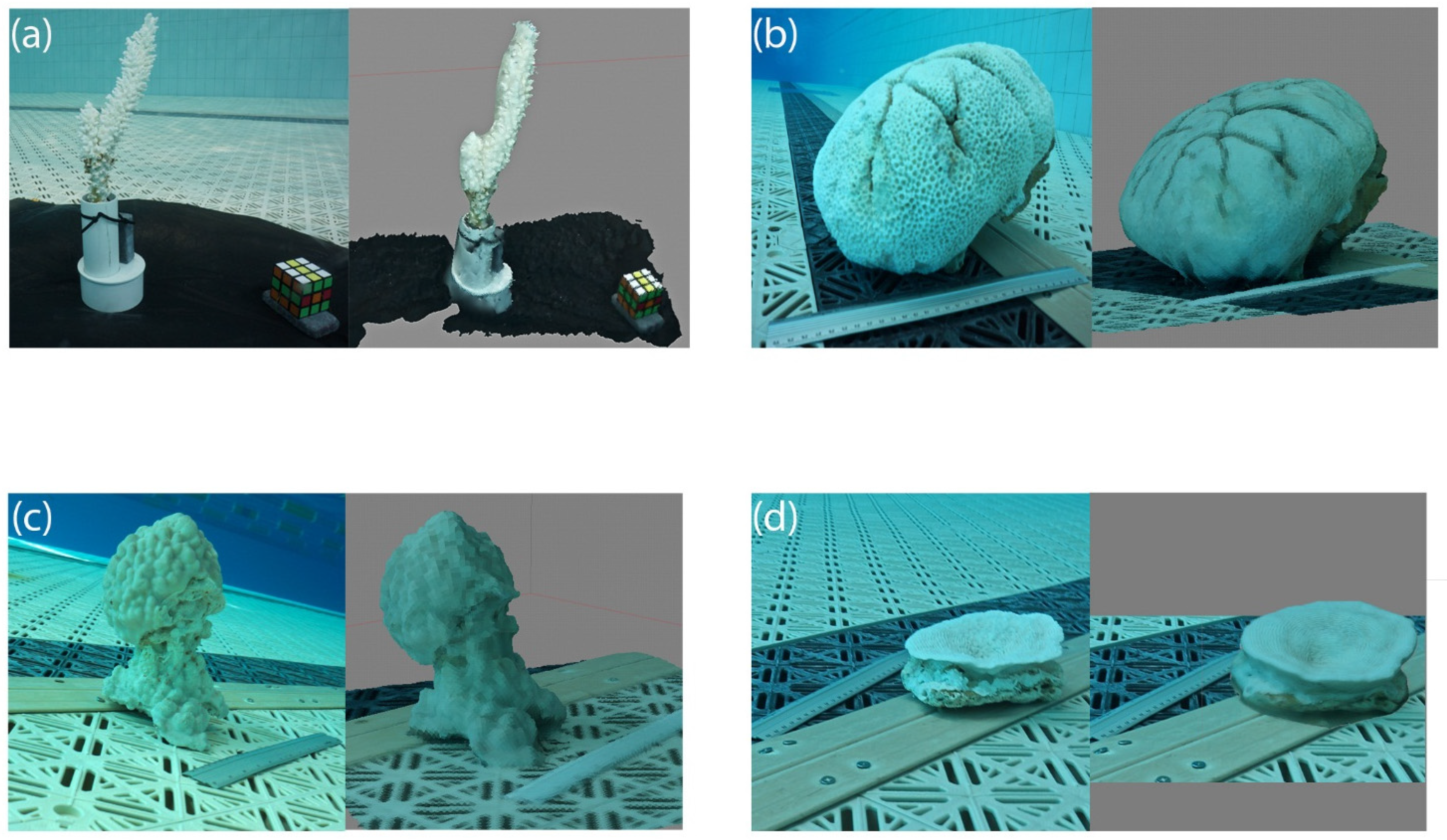
Figure 2. Examples of four of colonies used in this study showing a captured image (left panel) and the resulting fully textured model (right panel); (a) Bottlebrush; (b) Massive-medium (~30 cm diameter); (c) Massive-small (~12 cm diameter) and (d) Tabulate.
Remotesensing 07 15859 g002
A pilot study established that ~120 images was a suitable number to cover all perspectives required and enable reconstruction of a representative 3D model across a range of simple to complex coral morphologies. The image acquisition process involved placing the coral colony on the floor of the pool in a fixed position, similar to its natural orientation when attached to reef substratum, with a scale bar. Then, ~120 overlapping photographs at a rate of ~1 photo every 1–2 s with no flash were taken for each coral from different viewpoints using a standardised technique. The technique involved doing two 360° passes around the colony (~17 images per pass) and repeating this for distances of 1 m, 60 cm, and 30 cm away from the colony. Then a final two passes were done, in arcs directly over the top of the colony with the second being perpendicular to the first (~15 images per pass). Image acquisition took ~5–7 minutes per coral.

2.1.2. Patch-Scale

The focus for this work was on mapping larger areas of benthic habitat. For this study we used temperate rocky reefs as a focal system for the trials. An area of rocky subtidal reef at Shelly Beach in Sydney NSW, Australia was imaged using a custom-designed system. The habitat was at about 3–4 m depth and had a slope of about 45°. The mapping system consisted of an aluminium frame, 2 m long by 30 cm deep, to which three cameras were attached facing downward and equidistant apart (1 m between cameras). Cameras were GoPro Hero4 Black cameras (fixed F2.8 aperture, approx. 22 mm equivalent field of view, 1/2.3 inch sensor with 4000 × 3000 pixels) which were fitted with manufacturer underwater housing with a flat port.
Mapping was completed by first laying three to four visual references and two scale bars of known length (50 cm pvc cylinders marked at 10 cm intervals) over a ~20 m area of reef, and slowly (20 m/min) swimming the mapping rig at 2–3 m elevation over the bottom. The cameras were set to capture an image every second (wide field of view, 12 megapixel resolution). This protocol resulted in an image footprint size of approximately 5 m × 4 m and 80% overlap in imagery in the direction of travel. The whole system (all three cameras) covered a swath of approximately 7 m. Three passes were conducted in parallel to the transect line with the camera nearest to the previous pass having at least 50% overlap in image footprint with the nearest camera from the previous pass. Following this protocol, an area of approximately 200 m2 of reef was covered in approximately 10 min, generating 800–1000 images from the three cameras.

2.2. Model Building

The processing systems for colony and patch scale studies differed slightly but in both cases the 3D textured models were created from acquired images using a five step process: (1) aligning photos by feature detection and matching; (2) building of a sparse point cloud; (3) building of a dense point cloud; (4) mesh construction and (5) photo-texturing. This process was completed on Windows 7 workstations (minimum specifications of 64 bit OS, 64GB RAM, 2GB GPU, and quad-core 3.0 GHz CPU). Different processing systems were used for the patch and colony extent modeling as the purpose of this study was to evaluate precision and accuracy at each spatial extent using the types of tools currently being used and thus viewed as most appropriate for these different tasks. Each process is described below.

2.2.1. Colony-Scale

It is not uncommon for photogrammetry of features of the size of coral colonies to be undertaken using simple imaging systems (SLR or even point and shoot cameras) and small numbers of photos (10s–100s maximum) and so are amenable to modeling using free, open source software. We constructed models of the colonies using the free, open source software packages VisualSFM to build point clouds and MeshLab to generate meshes and do photo texturing. Feature detection in VisualSFM used a scale invariant feature transform (SIFT) algorithm [34] and generated a network of camera poses from which the sparse 3D point cloud of the model surface was generated. The sparse point cloud output is then processed by the Clustering Views for Multi-view Stereo (CMVS) package, which produces a much denser point cloud, which retains the colour information from the original image pixels. This package includes Patch-based Multi-view Stereo version 2 (PMVS2) which preserves only static structures in the point cloud, so any unwanted moving objects (e.g., fins, fish) that may have been photographed are excluded. PMVS2 is also impervious to any differences in image colour caused by exposure settings, lighting conditions, or white balance [35].
The dense point cloud was then imported into Meshlab where a polygon mesh was constructed using the Poisson Surface Reconstruction algorithm [36]. The scale bar in the image was used to scale the model into real units and then the scaled model was clipped to exclude anything other than the colony itself (such as the floor around the colony) and touched up by filling holes if needed. Finally, the photo-texture was projected onto the mesh using colour information from the original images (Figure 2, right panels). The final models had average (±SD) mesh resolutions (distance between neighbouring vertices) ranging from 1.2 mm (±0.40) to 2.8 mm (±0.57).

2.2.2. Patch-Scale

In contrast to the colony scale models, patch-scale modeling required more robust software solutions capable of processing 1000s of images and the automated elimination of non-static features in those images (mobile marine life and especially moving macroalgal habitat). Patch level models were reconstructed using the software package Photoscan Professional v1.1.6 (AgiSoft LLC). Photoscan uses a similar workflow as VisualSFM to build 3D models based on overlapping photos of the same areas from different angles and has been used in other studies which have modeled larger areas of benthic marine habitat as done here [16,19]. This process is highly dependent on the quality of photos, overlap between photos, and capturing all surfaces from multiple angles. First, photos are aligned by identifying common, invariant points, which results in a sparse point cloud in 3D space. This allows the software to calculate the location and orientation of cameras that took them. Second, alignment is optimized by the program based on camera and lense properties specified in image metadata. GoPro cameras set to wide produce barrel-distorted images. The Photoscan software accounts for this distortion with the “fit k4” alignment option in addition to the inbuilt lense distortion algorithms. Third, a dense cloud of points is generated by populating the sparse point cloud based on comon points in the photos and camera locations. Fourth, a mesh of three-sided polygons is built over the dense cloud to create a continuous 3D surface. Finally, a fitted texture is created by draping the original photos over the mesh. Specific settings are given in Table 1.
Table 1. Settings used for processing of patch-level models in Photoscan Professional (v1.1.6; Agisoft LLC).
ProcessParameter Choices
Align photosaccuracy low, pair preselection disabled, key point limit 40,000, tie point limit 1000, do not constrain features by mask
Optimize alignmentall properties yes, including fit k4
Build dense cloudmedium quality, mild depth filtering, do not reuse depth maps
Build mesharbritray surface type, source data-dense cloud face, count medium, interpolation enabled, all point classes
Build texturegeneric mapping mode, texture from all cameras, mosaic blending mode, texture size 4096, texture count 1, no color correction
The resulting models were clipped to exclude bordering areas of incomplete coverage and cleaned for obvious defects (e.g., detached components, holes, any bowl effect around edges). This process resulted in 3 meshs with an average (±SD) resolution of 30.3 (±2.82) mm each of which covered an area of approximately 200 m2. Model building took approximately 3 h of manual work plus 10 h of automated processing from photo collection to final mesh. This time was broken down into the following tasks (times approximate): 20 min of underwater photography (setup and mapping), 60 min of photo download and archiving, 30 min of model set-up, 10 h of automated model building, and 60 min of mesh checking, scaling, and cleaning.

2.3. Metric Derivation

For each model (coral colony or region of benthic habitat) we estimated the ratio of the 3D surface area to the 2D planar area (from the plane normal to the model), hereafter referred to as surface rugosity (SR). Surface rugosity is a metric similar to linear rugosity [37], but which accounts for the three-dimensional structural complexity of the coral [20]. This metric of complexity is commonly used in benthic remote sensing applications to assess bottom complexity, though typically over much larger spatial extents and at much lower resolutions [12].

2.4. Analyses of Precision and Accuracy

2.4.1. Colony-Scale

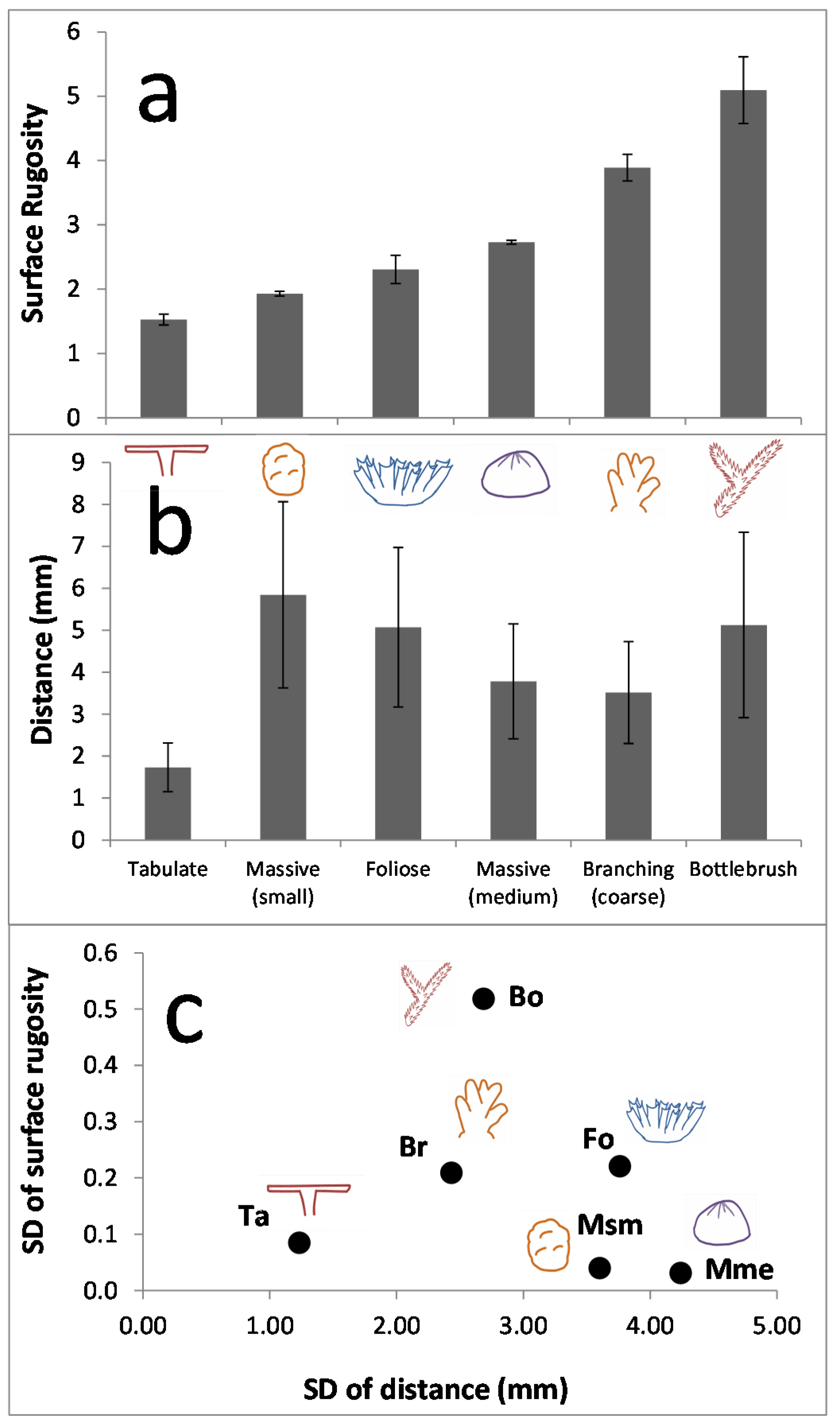
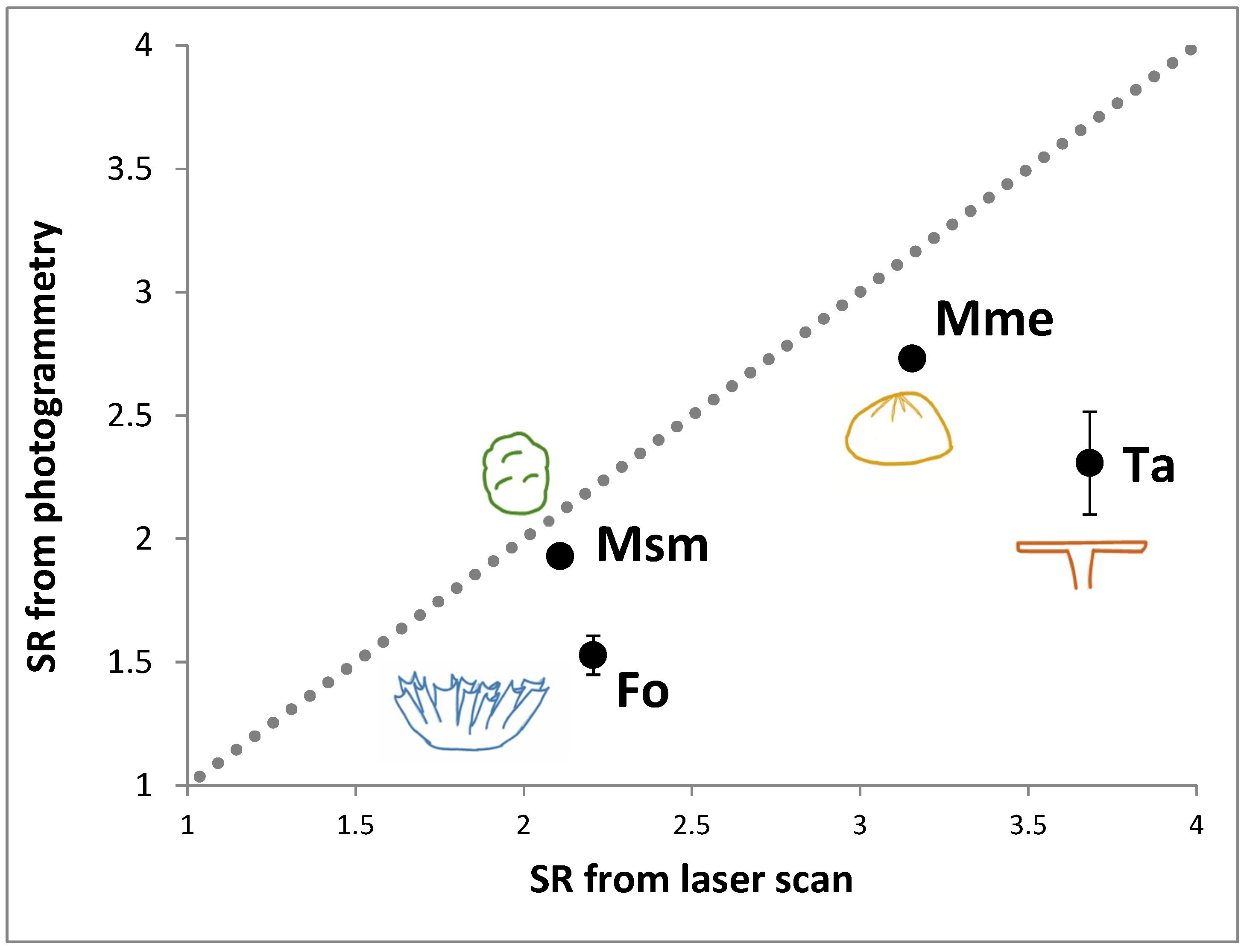
The precision with which coral colonies were modelled was assessed by repeatedly imaging and modelling one colony of each of the six morphologies 7 to 10 times (depending on morphology). We then derived SR estimates from each model and calculated their average, standard deviation (SD) and coefficient of variation (CV = 100 × average/SD) per morphology.
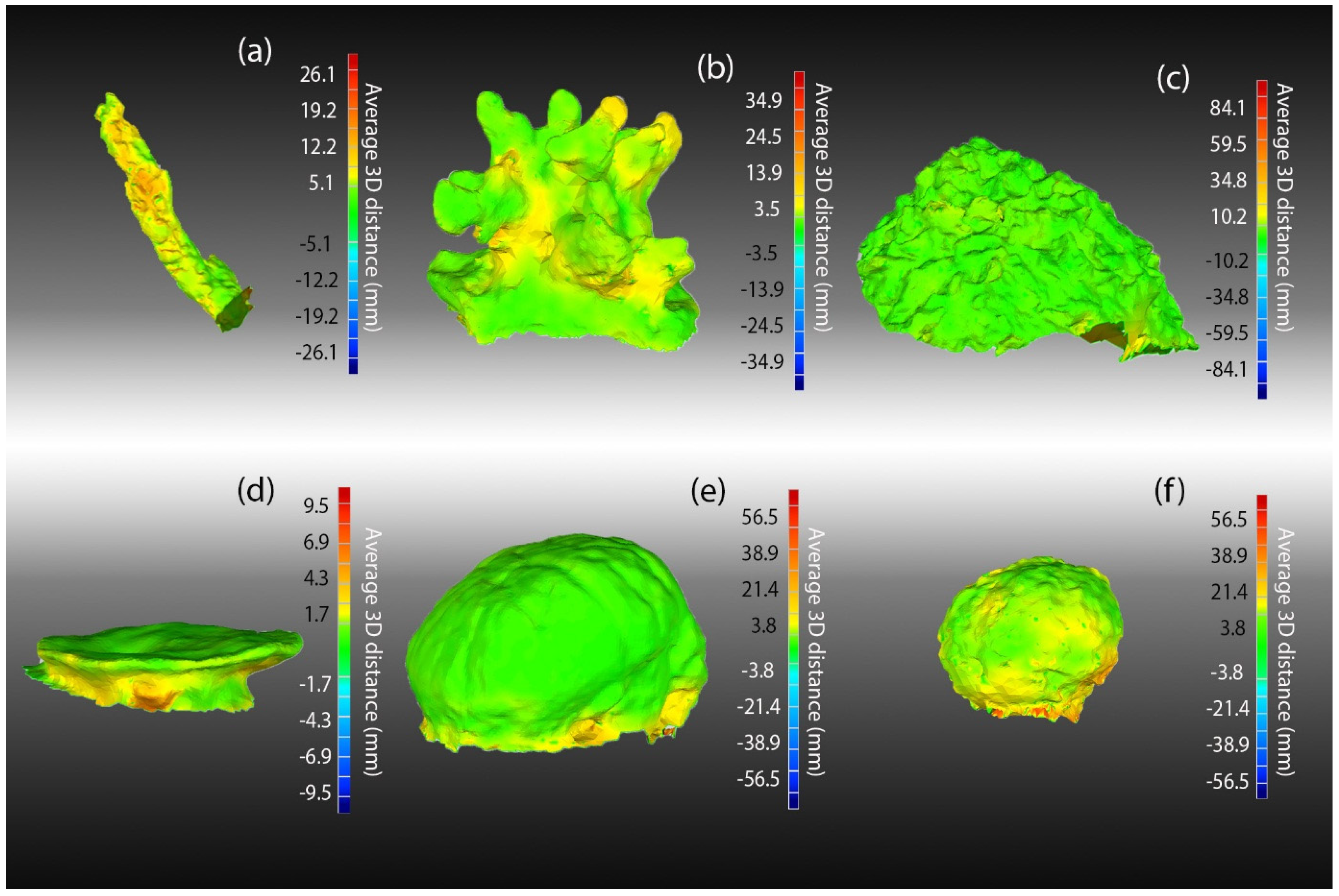
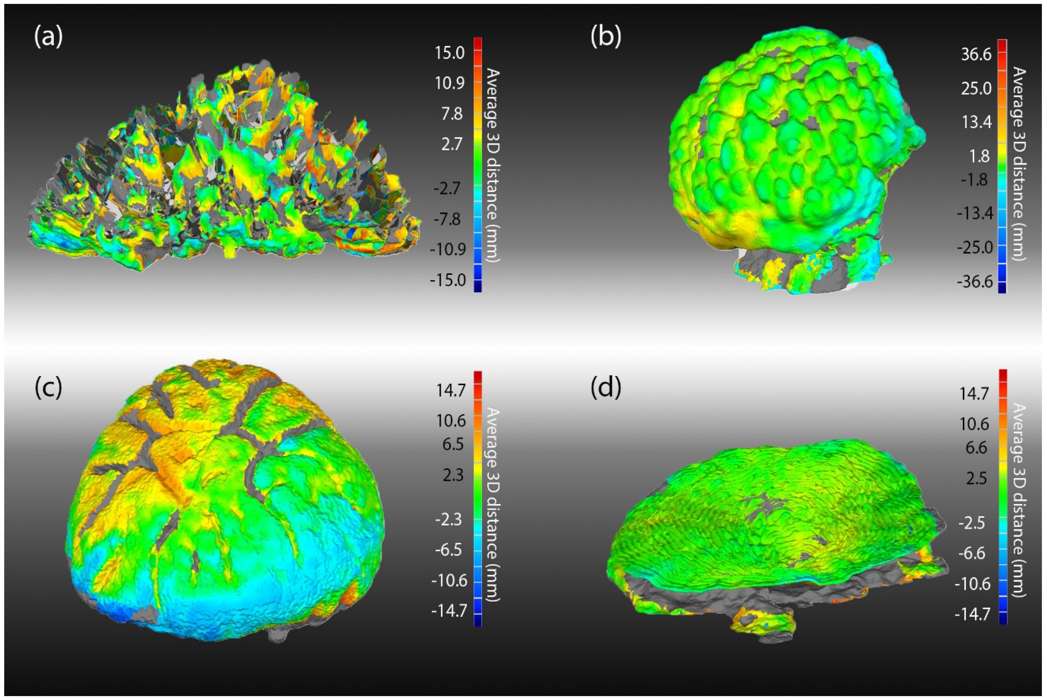
We also assessed differences in the geometry of 3D models using the “deviation analyses” tool in Geomagic Studio (3D Systems). The routine first aligned all models (“best fit algorithm”) for a morphology using best fit alignment and compared all models computing the average and SD of all distances between all pairs of models for all spatially matched points on the surface of each model. We evaluated the spatial distribution of these errors using heatmaps of these SD values overlaid on the average of all models per morph (using the “create average model” tool in Geomagic Studio).
Accuracy at the colony scale was assessed by comparing the average model from the repeated precision trials with that derived from laser scanning of the colony. Laser scanning was conducted by WYSIWYG 3D ® of Sydney Australia using a Nikon MMDx100 laser head, mounted on a Faro Platinum arm, with a combined system volumetric accuracy of ±0.05 mm. Real-time point cloud rendering captured the model at 0.2 mm resolution using Geomagic Studio point cloud software.
We compared the SR value from each photogrammetric model to that derived from the laser scan. From this we generated the average, SD and CV of the differences per morphology. We also used a Z-test (normal deviate) to test the hypothesis that the SR value from the laser scan model was not significantly different from that of all the models derived from photogrammetry.
The accuracy of model geometry was assessed by comparing the average model for each morphology with the laser scan using the “deviation analyses” tool in Geomagic Studio. The average model was created by aligning (“best-fit alignment”) all models for each morph and using Geomagic Studio’s “create average tool”. Accuracy was assessed as the average of the absolute value of all distances between all pairs of spatially matched points on the surface of each of the two models.

2.4.2. Patch-Scale

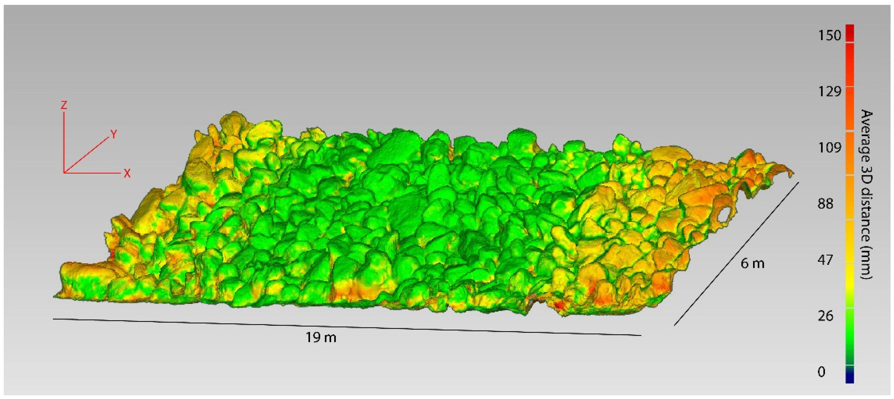
The precision of the patch-scale modelling technique was assessed by repeatedly mapping the exact same area of habitat three times over a period of one hour on the same day. Once rendered and cleaned (as described above), all models were imported into Geomagic Studio and precisely aligned using anchor points. The three models were then clipped to an area of about 120 m2 which was common to all three models. Model geometry was compared in Geomagic studio in the same manner outlined above for the colony scale. This process generated the average and SD of all distances between all pairs of models for all spatially matched points on the surface of each model.
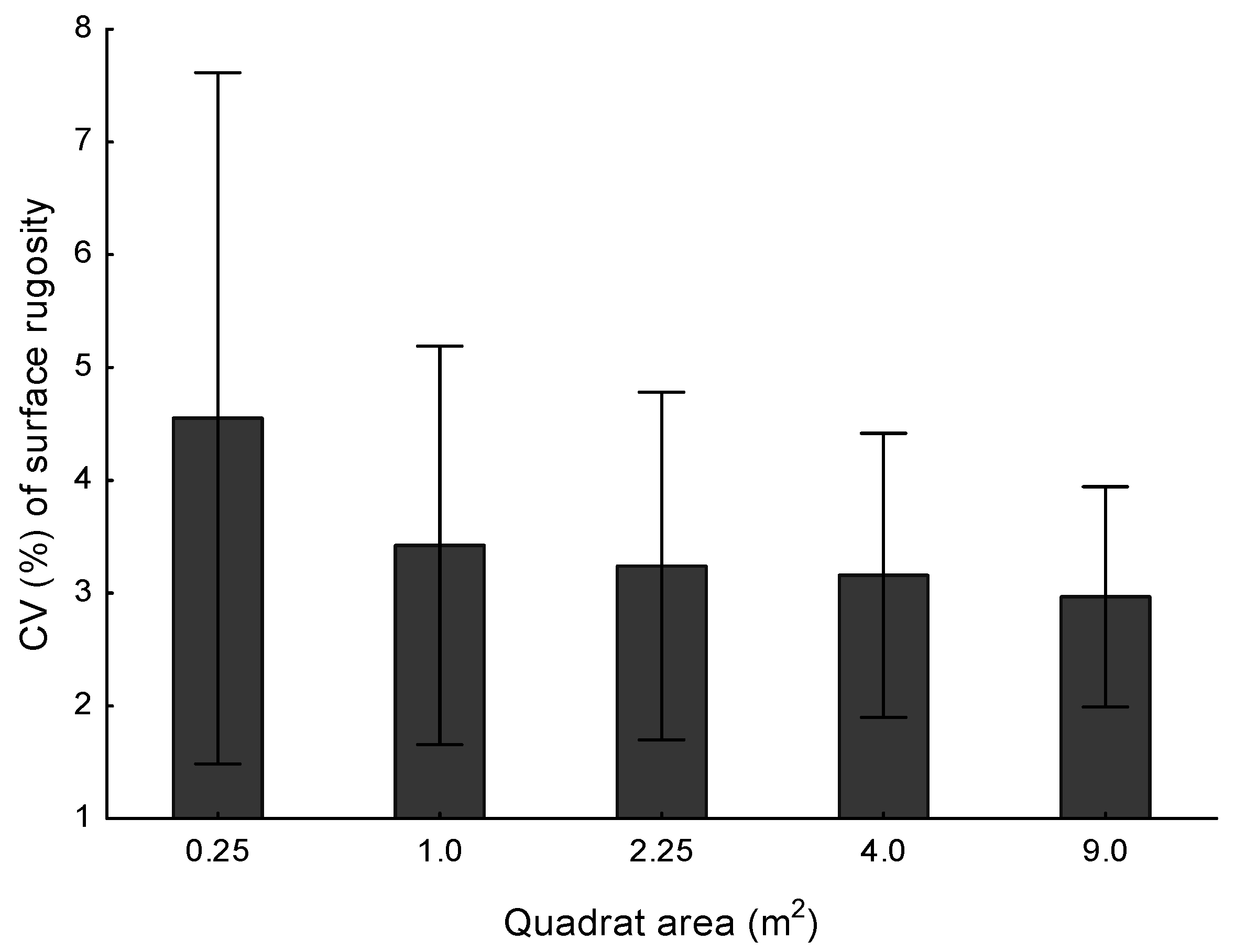
The precision of SR values derived from the models was assessed by uniformly sub sampling each mesh with a series of non-overlapping virtual quadrats in order to generate spatially matched (exact same area on all meshes) estimates of SR for each of these quadrats. This was done by first exporting each spatially aligned and clipped mesh from Geomagic in VRML (Virtual Reality Modeling Language) format, exporting the faces to X3D format using MeshLab (http://meshlab.sourceforge.net) and then conducting the spatial sub setting routine using a custom script in the Scala programming language (https://github.com/shawes/Mesh3D). The script first identified the largest maximum rectangle that fit within the bounding box of all three passes. Secondly, using coordinate geometry, this rectangle was sub-divided into approximately square (width and length provided as input), equal sized virtual quadrats. We then used a ray-casting algorithm to identify all faces whose centroid was inside a given virtual quadrat.
The 3D surface area of the mesh within each virtual quadrat was then calculated by summing the areas of all faces of the mesh that fell inside the quadrat. The surface rugosity within each virtual quadrat was then determined by dividing the 3D area by the 2D area of the same portion of the mesh. Because the mesh is made of triangular faces and the centroid was used to determine quadrat membership, the 2D projection of this mesh will not exactly fit within its nominally bounding virtual quadrat. The similarity of the 2D area of the virtual quadrat to that of the actual piece of mesh will decrease as the virtual quadrat size becomes closer to the resolution (internode distance) of the mesh. To avoid this dependence, we use the most accurate estimate of the 2D area of the piece of mesh of interest which is simply the sum of area of the 2D projection of all faces in a virtual quadrat onto the common 2D plane for the model. Note that there is no real-world data on the slope of the habitat in the model and as such, the 2D planar area of each quadrat is essentially based on a common plane-of-best-fit for the entire region. The approach of using a plane-of-best-fit when calculating surface roughness estimates such as this is generally favoured over the use of the true, real-world horizontal plane. This is because using plane-of-best-fit de-couples slope and SR, ensuring that change in elevation does not influence surface roughness calculations [20,38]. This approach was completed for five different nominal sizes of virtual quadrats, 0.25 m2, 1 m2, 2.25 m2, 4 m2, and 9 m2, giving sample sizes (number of non-overlapping quadrat which could be fit on the surface) of 456, 114, 48, 27, and 12 respectively.

3. Results

3.1. Colony-Scale Precision

The precision with which coral colonies were modeled with the DSLR camera system was generally high with average distances between 3D models ranging from 1–4 mm at any given point (Figure 3b and Figure 4, Table 2). However there was considerable variation in geometric similarity across the models as evident by the relatively large CV values of 50%–112%. The subsequent error around the SR estimates from these models was quite low and tended to increase for the more structurally complex morphologies like bottlebrush and branching (Figure 3a, Table 2). There was a general trend for a positive relationship between 3D geometry error and error in the resulting SR estimates for all morphs except for the two massive coral colony types, which showed consistently highly precise SR estimates, even when 3D geometry distances were elevated (Figure 3c).
Figure 3. Precision analysis of photogrammetrically derived 3D models of six morphotypes of coral colony. (a) Average (+/− SD) surface rugosity values for each morphology; (b) average (+/− SD) distance between all replicate models for each morphology based on comparison of 3D geometry; (c) comparisons of 3D geometry error (SD, x-axis) versus estimated surface rugosity error (SD, y-axis). Bb, Bottlebrush; Br, Branching-coarse; Fo, Foliose; Mme, Massive-medium; Msm, Massive-small; Ta, Tabulate.
Remotesensing 07 15859 g003
Table 2. Summary of precision analysis of coral colonies with the average and standard deviation from comparison on surface rugosity values from models, and the distance between the 3D models per morphology.
MorphologyModelsSurface Rugosity3D Distance (mm)
AVGSDCV%AvgSDCV%
Tabulate81.50.0845.51.71.2371.2
Massive (small)71.90.0392.05.83.6061.7
Foliose102.30.2209.55.13.7674.2
Massive (medium)102.70.0311.13.84.24112.2
Branching (coarse)93.90.2095.43.52.4469.3
Bottlebrush85.10.51810.25.12.6952.4
Figure 4. Precision analysis of 3D geometry of models of each morphology. The heatmap shows the spatial distribution of error (SD of average distance amongst models in mm) when all replicate models for each morphology were were compared using Geomagic Studio software deviation analysis. Morphologies are; (a) Bottlebrush; (b) Branching-coarse; (c) Foliose; (d) Tabulate; (e) Massive-medium; and (f) Massive-small. Areas where there was no model overlap are grey.
Remotesensing 07 15859 g004

3.2. Colony-Scale Accuracy

The accuracy of the models derived from photogrammetry (PG) was not high. While the actual distances between the laser scan and photogrammetry models was only 1.3–2.5 mm, on average there was a large spatial variation across the model in these differences such that the SD was the same or many times greater than the mean (Table 3). As a result, SR values differed by up to 38% from the laser reference model in the case of the foliose morphology. In general PG underestimated SR for all morphologies (Figure 5 and Figure 6) and Z-tests (normal deviate) indicated the LS (laser scanned) SR value was significantly different (alpha = 0.05) from those derived from PG for all morphologies (Table 3).
Figure 5. Comparison of the surface rugosity (SR) values derived from 3D models determined from laser scanning with the average (+/− SD) SR from all replicate models determined from photogrammetry for four coral morphotypes. Dashed line is 1:1, points under this line indicate where SR is underestimated by photogrammetry. Morphologies are: Fo, Foliose; Mme, Massive-medium; Msm, Massive-small; Ta, Tabulate.
Remotesensing 07 15859 g005
Figure 6. Accuracy analysis of 3D models of each morphology. The heatmap shows the distance (mm) between the laser scan reference model and the average (of all replicates) model for each morphology: (a) Foliose; (b) Massive-small; (c) Massive-medium; and (d) Tabulate. Areas where there was no model overlap are indicated in grey.
Remotesensing 07 15859 g006
Table 3. Summary of small-scale accuracy assessment. The average (AVG), percent (%, relative to LS), SD and CV (%) of the difference in surface rugosity between the laser scan (LS) and each photogrammetry (PG) model as well as results of the normal deviate test (Z-test) are given for each morphology. The average, SD and CV (%) of the distance between the LS 3D model and the average of all PG models is also given.
MorphologyMod.Surface Rugosity–Difference from LSLS-PG Comparison3D Distance (mm)
LSAVG%SDCV%Zp (Z)AvgSDCV%
Tabulate82.210.6830.70.07911.78.58<0.012.53.42137.1
Massive (sm)72.110.188.50.03620.24.96<0.010.93.47383.5
Foliose103.681.3837.40.20915.26.59<0.012.76.03226.2
Massive (med)103.160.4213.50.0296.814.66<0.012.34.60197.0

3.3. Patch-Scale Precision

Comparison of the three models indicated they were, on average, about 25 mm different in most spots (Table 4). In some of the more complex areas however, this difference was ~90 mm (Figure 7). The SRs value estimated for the whole area differing by only a few percent in absolute value among the three models (Table 4). There was spatial variability in the precision with which SR was estimated but the magnitude of this variability did depend somewhat on the quadrat size used to calculate it. Using 0.25 m2 quadrats gave higher estimates of error in some regions leading to a higher overall average error value for the domain and a greater spread of values (Figure 8), though at 4.5% CV, the error is relatively low. For quadrat areas greater than this, the average error was smaller and quite similar, ranging between 3%–3.5%. Looking more closely at the quadrat size with the most replicates within this stable range, 1 m2, its clear that there are specific areas of the domain where error rates were much higher (Figure 9). These areas of low precision do not seem to be especially structurally complex based on a non-significant regression of the average SR (independent) against the CV of all SR values (dependent) for each 1 m2 quadrat (t112 = −0.120, p = 0.91, r2 = 0.001).
Figure 7. Precision analysis patch-scale models showing the spatial distribution of error (average distance, mm) among all replicate models.
Remotesensing 07 15859 g007
Table 4. Summary of patch-level precision analysis giving the average and SD surface rugosity (SR) values derived from the three replicate models as well as the average, SD, and CV (%) of the 3D distance (mm) between those models from comparisons of geometry.
SR3D Dist. (mm).
Average1.7525.0
SD0.06819.9
CV (%)3.979.6
Figure 8. Average (±S.D.) precision (CV) in surface rugosity (SR) estimates amongst models derived from replicate photogrammetric modelling of a 120 m2 area of benthic habitat. A grid of non-overlapping virtual square quadrats of a specific area was laid over the model domain and the variation in the mean SR value from each of the three models in a quadrat was calculated. This process was done for five different quadrat areas. Sample sizes were 456, 114, 48, 27, and 12 for 0.25, 1, 2.25, 4, and 9 m2 quadrats, respectively.
Remotesensing 07 15859 g008
Figure 9. Spatial distribution of precision (CV) in surface rugosity (SR) values amongst three models derived from replicate photogrammetric modelling of a 120 m2 area of benthic habitat. Error in SR values was calculated from the same spatial area of each aligned model based on a grid of non-overlapping virtual square quadrats of 1 m2 area laid over the model domain.
Remotesensing 07 15859 g009

4. Discussion

This study evaluated the precision and accuracy of metrics derived from photogrammetric 3D models of individual coral colonies as well as a 120 m2 area of reef. Precision was assessed for six coral morphotypes; while accuracy was evaluated for a subset of four of these. Surface rugosity measurements were generally precise across all morphotypes and spatial extents with average differences in the geometry of replicate models of 1–6 mm for coral colonies and 25 mm for the reef area. Precision decreased as the complexity of the coral increased, with SR for medium massive corals being the most precise (1% CV in surface rugosity) and metrics for bottlebrush corals being the least precise (10% CV in surface rugosity). There was no indication however that precision was related to complexity for the patch-scale modelling. The 3D geometry of coral models differed by only 1–3 mm from laser reference models however high spatial variation in these differences around the model led to a consistent underestimation of surface rugosity values for all morphs of between 8% and 37%. Overall, this study demonstrated two fit-for-purpose approaches to the assessment of structural complexity of benthic marine systems for application at two commonly investigated spatial extents using off-the-shelf camera systems and readily available, consumer quality, and in some cases, free software tools. The results of the precision and accuracy assessments of these systems will allow for an appraisal of their utility for different tasks.

4.1. Colony-Scale

There was a wide range of SR values estimated for the six coral morphotypes and, while there was a strong inverse relationship between SR and precision, the repeatability of the derived complexity metric was high, with CV from repeated trials being 10% at the worst for the most complex morphology. This result is similar to the 1%–5% error (CV) estimated by Lavy et al. [28] for Stylophora (branching morphology), one of the few studies to have assessed precision in photogrammetrically derived 3D models of corals. Lavy et al. [28] focused on volume and surface area rather than SR. However as SR is derived from surface area, a similar response of the two metrics is to be expected. Our comparisons of model geometry allowed us to confirm that the low SR error was the result of the general similarity in the 3D geometry of the derived models, which only differed by 1–4 mm on average. The effect of SR on error is likely due to the inability of the modeling system to adequately capture the fine-scale surface texture when it varies at scales that approach the roughly 3 mm mesh resolution of the coral colony models. For instance, bottlebrush texture is formed by the coralites which tend to be smaller than 2 mm, explaining the low precision and accuracy for this morphology in particular. The interaction of mesh resolution with the scale of surface roughness is of fundamental importance when selecting the modeling system and approach to use for a given application.
While precision was high, the accuracy of the coral models to the reference was less so. The models only differed from the laser reference model by a few millimeters but there was considerable variability in this distance across the topology of the models (CVs of 137%–383%). As a result, SR values varied by between 10% and 40% from the reference model. While few other studies have looked at accuracy of SR, these values are actually consistent with the range in bias in estimates of both surface area (1%–78%) and volume (2%–24%) from other studies using photogrammetry to model a variety of different coral morphotypes [25,26,27,28,29]. An important question in any assessment of bias is the accuracy of the reference value itself. These studies used conventional methods to assess surface area and volume such as foil-wrap, wax drip, and volume displacement while the reference model used in the present study was generated by laser scanning and had a 0.2 mm mesh resolution. The estimate of structural complexity used here, SR, requires the surface area of the model to be estimated for its calculation. We would expect the laser scan model to deliver a more accurate estimate of surface area than conventional methods like foil-wrap and wax drip and thus potentially inflating the bias in estimates of SR from photogrammetry with respect to previous studies. This more accurate estimate of 3D surface area in the laser scan probably also explains the tendency for photogrammetry to underestimate SR for all morphologies examined.

4.2. Patch Scale

The application of photogrammetry to the assessment of complexity at spatial extents larger than coral heads is a significant step. The extensive literature in which the structural complexity of benthic habitats is estimated using a variety of techniques is testament to its importance as a predictor of the distribution and abundance of organisms (reviews, [1,5]). Here we have demonstrated that it is possible to map a 120 m2 area of reef in less than 20 min using relatively inexpensive off-the-shelf camera systems. This imagery was processed using readily available software and delivered a model mesh with a resolution of approximately 30 mm. Replicate models of the same area differed by about 25 mm on average and the CV on the estimates of SR were very low, 4%. While there was spatial variability in the SR estimates across the modeled patch, this was not associated with the structural complexity of those regions. Much of the high variation was in a shallow and more wave-exposed part of the patch. It is likely that increased surge in this region led to reduced image quality and therefore a less detailed sparse point cloud resulting from fewer feature matches. This highlights the fact that careful consideration of the image capture methodology and conditions can often be as important as the underlying quality of the hardware and software used in the process.
While this work was completed in a temperate rather than a tropical reef, the principle of application is the same. Indeed the increased visibility of tropical waters is quite likely to improve the texturing and mesh resolution. While the underlying structural complexity of the habitat mapped here (SR ~2) was similar to that estimated for coral reefs by the few other studies which have employed photogrammetry over these sorts of spatial scales [1,2,3,4,16,19,32], the temperate rocky habitat mapped in this study was likely more homogenous than the reef in these other studies. What effect, if any, this would have on precision estimates is unclear and would need to be evaluated in a similar manner in future studies to that conducted here.

4.3. Implications for Monitoring

The benefits of the photogrammetry and structure from motion approach used here are becoming increasingly clear. The technique is non-invasive and can be much more cost effective than gathering the same quality data on habitat structural complexity in other ways (e.g., chain and tape, counting holes etc.). The technique is proving quite valuable for assessing characteristics of small features like corals and improvements in processing and data acquisition hardware and techniques should lead to improvements in accuracy. It is important to mention that better accuracies are achievable, especially at larger extents, by custom built systems with additional telemetry and purpose designed processing software [39] however these are typically very expensive and are not readily available to most researchers worldwide. While accuracy is important, for many applications of this technology, such as long-term monitoring, repeatability or precision is perhaps equally or more important. Indeed 3D modeling of coral habitats using photogrammetry has been identified as a key improvement to traditional monitoring programs [40]. The present study indicated that the small-scale approach would be capable of detecting changes in the physical height of the benthic habitat of about 5 mm while the patch-scale technique would be 25 mm. It is difficult to characterize linear growth rates for corals in general though detailed studies of the more slowly growing massive morphology Porities indicates rates of 10–15 mm per year are not uncommon on the Great Barrier Reef [41]. Such rates of growth would be detected by the SLR-based system within a year but it would take longer to pick them up with the GoPro-based one in this study. Of course the GoPro-based system is capable of coving a much larger area than the SLR based one and thus, even with its lower resolution, could be more appropriate for distinguishing differences in structural complexity amongst different habitat types where the morphological composition of coral communities differs. Thus, an understanding of precision makes it possible to choose a system which will provide the best spatial coverage with respect to the funds available but will also allow for detection of ecologically relevant rates of change in structural complexity over time frames relevant to important ecological processes and management.
We focused on comparison of 3D model structure and that of the derived metric, surface rugosity. It is important to note that these are but a few of the many different metrics of structural complexity which have been proposed. SR is a good choice in that it has a direct analog in traditional linear rugosity [37] which has been used for nearly 50 years to quantify the structural complexity of habitat. It has also been demonstrated to be superior to this traditional approach when applied to modeled habitat as its not sensitive to the specific placement in 2D space of the measured transect [20]. However, other approaches, such as variance in height [17], slope, or even fractal dimension [16,42,43] may also prove useful as descriptors of structural complexity.

5. Conclusions

There is an increasing need to better capture and describe the structural complexity of benthic marine systems, especially coral reefs, in order to monitor anthropogenic impacts on them and make predictions on ecosystem trajectories that may inform monitoring and management programs. This study presents two approaches tailored to assess the structural complexity of habitat at small (coral colony) and medium (100’s·m2) spatial extents. Both approaches use off-the-shelf hardware and software components and proved to be repeatable. The information provided by these analyses in concert with expectations about the magnitudes and extent of structural complexity can be used to inform the best choice of system for the application.

Acknowledgments

This work was funded in part by a University of Sydney Faculty of Science Research Equipment and Infrastructure Grant to Will Figueira, Renata Ferrari, and Maria Byrne and a grant from the Great Barrier Reef Foundation under the Foundation’s Resilient Coral Reefs Successfully Adapting to Climate Change research program. We thank the Australian Museum for access to the coral specimens and WYSIWYG 3D® of Sydney Australia for supporting this project. This is contribution 169 to the Sydney Institute of Marine Science.

Author Contributions

Will Figueira, Renata Ferrari, Elyse Weatherby, and Augustine Porter conceived and designed the experiment. Elyse Weatherby, Augustine Porter, and Renata Ferrari conducted imaging and modeling. Will Figueira, Renata Ferrari, Elyse Weatherby and Steven Hawes conducted data analysis and summary. Will Figueira, Elyse Weatherby, Renata Ferrari, Augustine Porter, and Maria Byrne contributed to the writing of the manuscript.

Conflicts of Interest

The authors declare no conflict of interest.

References

  1. Kovalenko, K.E.; Thomaz, S.M.; Warfe, D.M. Habitat complexity: Approaches and future directions. Hydrobiologia 2011, 685, 1–17. [Google Scholar] [CrossRef]
  2. Matias, M.G.; Underwood, T.; Hochuli, D.F.; Coleman, R.A. Habitat identity influences species-area relationships in heterogeneous habitats. Mar. Ecol. Prog. Ser. 2011, 437, 135–145. [Google Scholar] [CrossRef]
  3. Figueira, W.; Lyman, S.; Crowder, L.; Rilov, G. Small-scale demographic variability of the biocolor damselfish, stegastes partitus, in the florida keys USA. Environ. Biol. Fishes 2008, 81, 297–311. [Google Scholar] [CrossRef]
  4. Meager, J.J.; Schlacher, T.A. New metric of microhabitat complexity predicts species richness on a rocky shore. Mar. Ecol. 2013, 34, 484–491. [Google Scholar] [CrossRef]
  5. Graham, N.A.J.; Nash, K.L. The importance of structural complexity in coral reef ecosystems. Coral Reefs 2012, 32, 315–326. [Google Scholar] [CrossRef]
  6. Rogers, A.; Blanchard, J.L.; Mumby, P.J. Vulnerability of coral reef fisheries to a loss of structural complexity. Curr. Biol. 2014, 24, 1000–1005. [Google Scholar] [CrossRef] [PubMed]
  7. Catano, L.; Gunn, B.; Kelley, M.; Burkepile, D. Predation risk, resource quality, and reef structural complexity shape territoriality in a coral reef herbivore. PLoS ONE 2015, 10. [Google Scholar] [CrossRef] [PubMed]
  8. Bozec, Y.M.; Alvarez-Filip, L.; Mumby, P.J. The dynamics of architectural complexity on coral reefs under climate change. Glob. Chang. Biol. 2015, 21, 223–235. [Google Scholar] [CrossRef] [PubMed]
  9. Munday, P.L.; Jones, G.P.; Pratchett, M.S.; Williams, A.J. Climate change and the future for coral reef fishes. Fish Fish. 2008, 9, 261–285. [Google Scholar] [CrossRef]
  10. Wedding, L.M.; Friedlander, A.M.; McGranaghan, M.; Yost, R.S.; Monaco, M.E. Using bathymetric lidar to define nearshore benthic habitat complexity: Implications for management of reef fish assemblages in hawaii. Remote Sens. Environ. 2008, 112, 4159–4165. [Google Scholar] [CrossRef]
  11. Knudby, A.; Jupiter, S.; Roelfsema, C.; Lyons, M.; Phinn, S. Mapping coral reef resilience indicators using field and remotely sensed data. Remote Sens. 2013, 5, 1311–1334. [Google Scholar] [CrossRef]
  12. Moore, C.H.; Harvey, E.S.; van Niel, K. The application of predicted habitat models to investigate the spatial ecology of demersal fish assemblages. Mar. Biol. 2010, 157, 2717–2729. [Google Scholar] [CrossRef]
  13. Bejarano, S.; Mumby, P.J.; Sotheran, I. Predicting structural complexity of reefs and fish abundance using acoustic remote sensing (RoxAnn). Mar. Biol. 2011, 158, 489–504. [Google Scholar] [CrossRef]
  14. Negahdaripour, S. On 3-D motion estimation from feature tracks in 2-D fs sonar video. IEEE Trans. Robot. 2013, 29, 1016–1030. [Google Scholar] [CrossRef]
  15. Aykin, M.D.; Negahdaripour, S. On feature matching and image registration for two-dimensional forward-scan sonar imaging. J. Field Robot. 2013, 30, 602–623. [Google Scholar] [CrossRef]
  16. Leon, J.X.; Roelfsema, C.M.; Saunders, M.I.; Phinn, S.R. Measuring coral reef terrain roughness using “structure-from-motion” close-range photogrammetry. Geomorphology 2015, 242, 21–28. [Google Scholar] [CrossRef]
  17. Harborne, A.R.; Mumby, P.J.; Ferrari, R. The effectiveness of different meso-scale rugosity metrics for predicting intra-habitat variation in coral-reef fish assemblages. Environ. Biol. Fishes 2012, 94, 431–442. [Google Scholar] [CrossRef]
  18. Harborne, A.R.; Mumby, P.J.; Kennedy, E.V.; Ferrari, R. Biotic and multi-scale abiotic controls of habitat quality: Their effect on coral-reef fishes. Mar. Ecol. Prog. Ser. 2011, 437, 201–214. [Google Scholar] [CrossRef]
  19. Burns, J.H.R.; Delparte, D.; Gates, R.D.; Takabayashi, M. Integrating structure-from-motion photogrammetry with geospatial software as a novel technique for quantifying 3D ecological characteristics of coral reefs. PeerJ 2015, 3. [Google Scholar] [CrossRef] [PubMed]
  20. Friedman, A.; Pizarro, O.; Williams, S.B.; Johnson-Roberson, M. Multi-scale measures of rugosity, slope and aspect from benthic stereo image reconstructions. PLoS ONE 2012, 7. [Google Scholar] [CrossRef] [PubMed]
  21. O’Byrne, M.; Pakrashi, V.; Schoefs, F.; Ghosh, B. A comparison of image based 3D recovery methods for underwater inspections. In Proceedings of the 7th European Workshop on Structural Health Monitoring, Nantes, France, 8–14 July 2014.
  22. McCarthy, J.; Benjamin, J. Multi-image photogrammetry for underwater archaeological site recording: An accessible, diver-based approach. J. Mar. Arch. 2014, 9, 95–114. [Google Scholar] [CrossRef]
  23. Gonzalez-Rivero, M.; Bongaerts, P.; Beijbom, O.; Pizarro, O.; Friedman, A.; Rodriguez-Ramirez, A.; Upcroft, B.; Laffoley, D.; Kline, D.; Bailhache, C.; et al. The catlin seaview survey—Kilometre-scale seascape assessment, and monitoring of coral reef ecosystems. Aquat. Conserv. Mar. Freshw. Ecosyst. 2014, 24, 184–198. [Google Scholar] [CrossRef]
  24. Beck, M.W. Comparison of the measurement and effects of habitat structure on gastropods in rocky intertidal and mangrove habitats. Mar. Ecol. Prog. Ser. 1998, 169, 165–178. [Google Scholar] [CrossRef]
  25. Bythell, J.; Pan, P.; Lee, J. Three-dimensional morphometric measurements of reef corals using underwater photogrammetry techniques. Coral Reefs 2001, 20, 193–199. [Google Scholar]
  26. Cocito, S.; Sgorbini, S.; Peirano, A.; Valle, M. 3-D reconstruction of biological objects using underwater video technique and image processing. J. Exp. Mar. Biol. Ecol. 2003, 297, 57–70. [Google Scholar] [CrossRef]
  27. Courtney, L.A.; Fisher, W.S.; Raimondo, S.; Oliver, L.M.; Davis, W.P. Estimating 3-dimensional colony surface area of field corals. J. Exp. Mar. Biol. Ecol. 2007, 351, 234–242. [Google Scholar] [CrossRef]
  28. Lavy, A.; Eyal, G.; Neal, B.; Keren, R.; Loya, Y.; Ilan, M.; McMahon, S. A quick, easy and non-intrusive method for underwater volume and surface area evaluation of benthic organisms by 3D computer modelling. Methods Ecol. Evol. 2015, 6, 521–531. [Google Scholar] [CrossRef]
  29. Gutierrez-Heredia, L.; D’Helft, C.; Reynaud, E.G. Simple methods for interactive 3D modeling, measurements, and digital databases of coral skeletons. Limnol. Oceanogr. Methods 2015, 13, 178–193. [Google Scholar] [CrossRef]
  30. McKinnon, D.; Hu, H.; Upcroft, B.; Smith, R. Towards automated and in-situ, near-real time 3-D reconstruction of coral reef environments. In Proceedings of the OCEANS 2011, Waikoloa, HI, USA, 19–22 September 2011; pp. 1–10.
  31. Pizarro, O.; Eustice, R.M.; Singh, H. Large area 3-D reconstructions from underwater optical surveys. IEEE J. Ocean. Eng. 2009, 34, 150–169. [Google Scholar] [CrossRef]
  32. He, H.; Ferrari, R.; McKinnon, D.; Roff, G.A.; Smith, R.; Mumby, P.J.; Upcroft, B. Measuring reef complexity and rugosity from monocular video bathymetric reconstruction. In Proceedings of the 12th International Coral Reef Symposium, Cairns, Australis, 9–13 July 2012.
  33. Laforsch, C.; Christoph, E.; Glaser, C.; Naumann, M.; Wild, C.; Niggl, W. A precise and non-destructive method to calculate the surface area in living scleractinian corals using X-ray computed tomography and 3D modeling. Coral Reefs 2008, 27, 811–820. [Google Scholar] [CrossRef]
  34. Lowe, D.G. Distinctive image features from scale-invariant keypoints. Int. J. Comput. Vis. 2004, 60, 91–110. [Google Scholar] [CrossRef]
  35. Favalli, M.; Fornaciai, A.; Isola, I.; Tarquini, S.; Nannipieri, L. Multiview 3D reconstruction in geosciences. Comput. Geosci. UK 2012, 44, 168–176. [Google Scholar] [CrossRef] [Green Version]
  36. Kazhdan, M.M.; Bolitho, M.; Hoppe, H. Screened poisson surface reconstruction. ACM Trans. Graph. 2006, 32, 61–70. [Google Scholar] [CrossRef]
  37. Risk, M.J. Fish diversity on a coral reef in the virgin islands. Atoll Res. Bull. 1972, 153, 1–6. [Google Scholar] [CrossRef]
  38. Du Preez, C. A new arc-chord ratio (ACR) rugosity index for quantifying three-dimensional landscape structural complexity. Landsc. Ecol. 2014, 30, 181–192. [Google Scholar] [CrossRef]
  39. Johnson-Roberson, M.; Pizarro, O.; Williams, S.B.; Mahon, I. Generation and visualization of large-scale three-dimensional reconstructions from underwater robotic surveys. J. Field Robot. 2010, 27, 21–51. [Google Scholar] [CrossRef]
  40. Zapata-Ramírez, P.A.; Scaradozzi, D.; Sorbi, L.; Palma, M.; Pantaleo, U.; Ponti, M.; Cerrano, C. Innovative study methods for the mediterranean coralligenous habitats. Adv. Oceanogr. Limnol. 2013, 4, 102–119. [Google Scholar] [CrossRef]
  41. De’ath, G.; Lough, J.M.; Fabricius, K.E. Declining coral calcification on the great barrier reef. Science 2009, 323, 116–119. [Google Scholar] [CrossRef] [PubMed]
  42. Parrott, L. Measuring ecological complexity. Ecol. Indic. 2010, 10, 1069–1076. [Google Scholar] [CrossRef]
  43. Kamal, S.; Lee, S.Y.; Warnken, J.; McMahon, S. Investigating three-dimensional mesoscale habitat complexity and its ecological implications using low-cost rgb-d sensor technology. Methods Ecol. Evol. 2014, 5, 845–853. [Google Scholar] [CrossRef]

