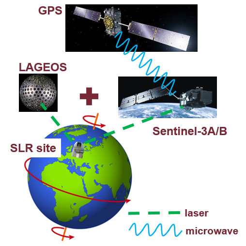
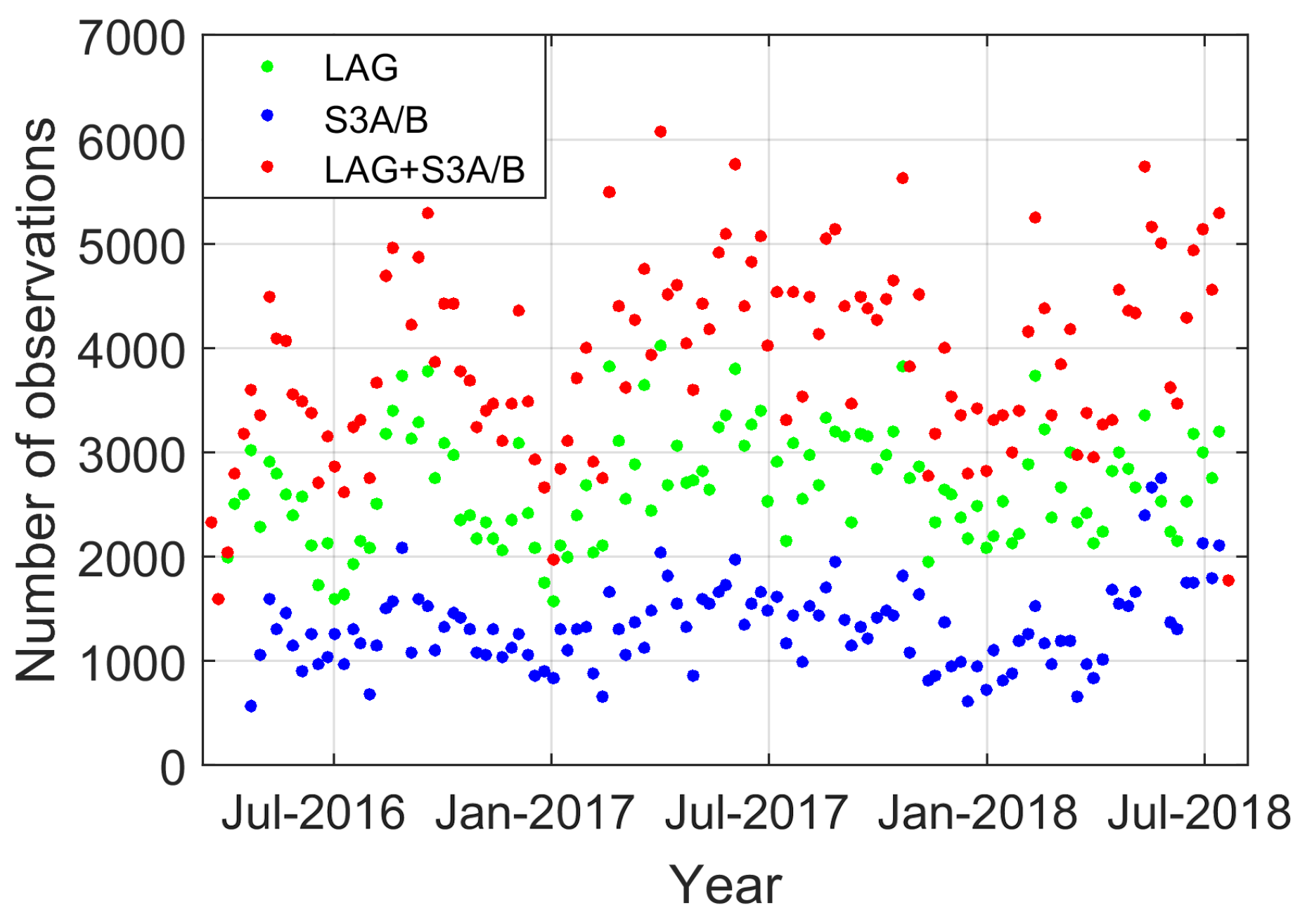
Figure 1.
Satellite Laser Ranging (SLR) observations to S3A/B and LAG in 7-day batches.
Figure 1.
Satellite Laser Ranging (SLR) observations to S3A/B and LAG in 7-day batches.
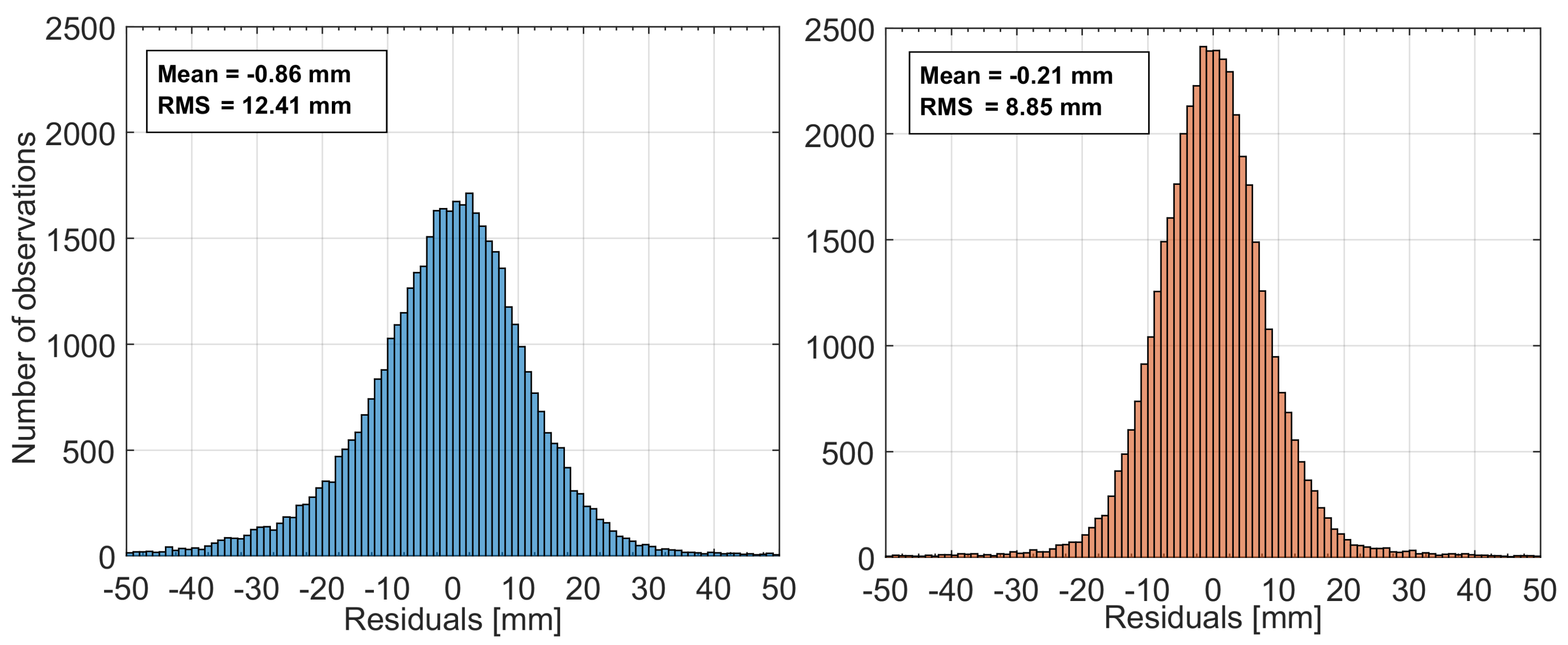
Figure 2.
Residual histograms for solutions with uncorrected (left) and corrected (right) range biases for all sites.
Figure 2.
Residual histograms for solutions with uncorrected (left) and corrected (right) range biases for all sites.
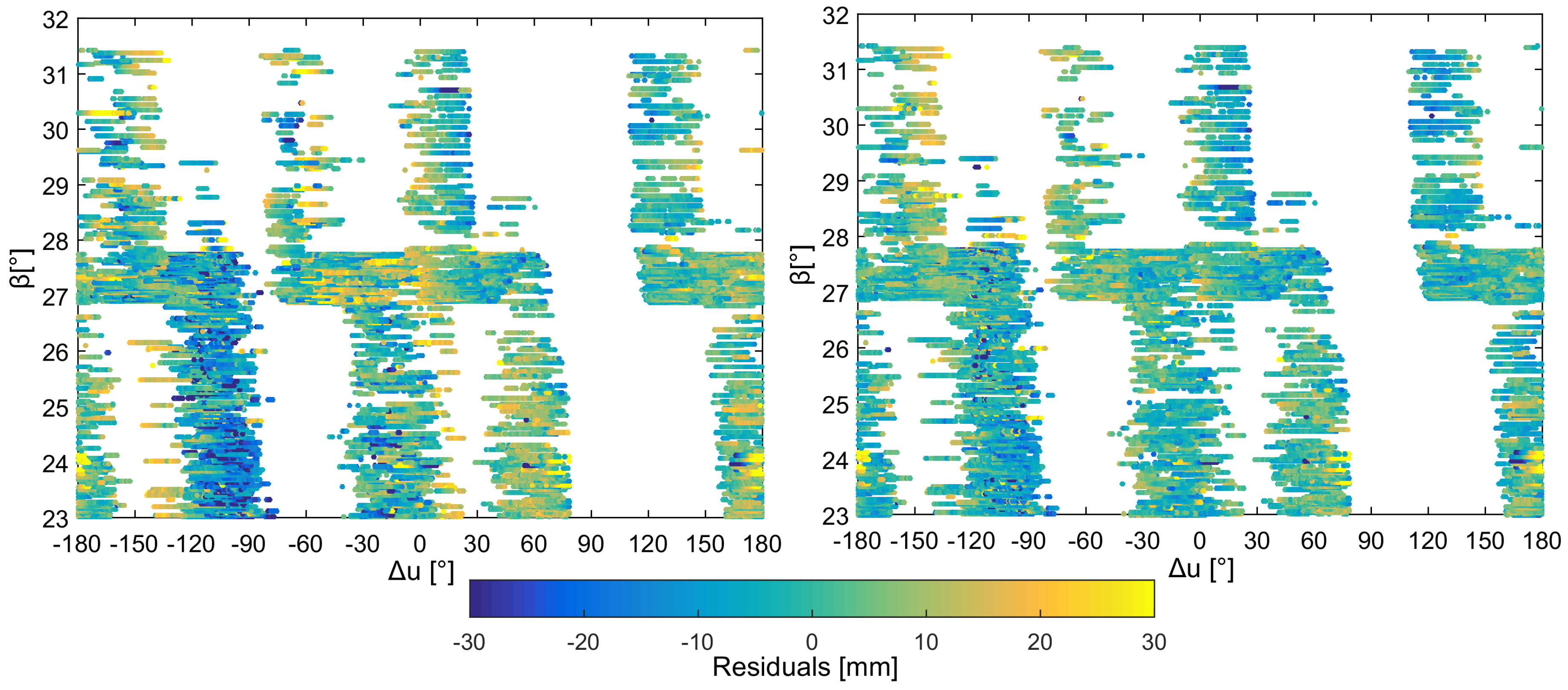
Figure 3.
Dependency of residuals on S3A as a function of and u angles for solutions with uncorrected (left) and corrected (right) range biases.
Figure 3.
Dependency of residuals on S3A as a function of and u angles for solutions with uncorrected (left) and corrected (right) range biases.
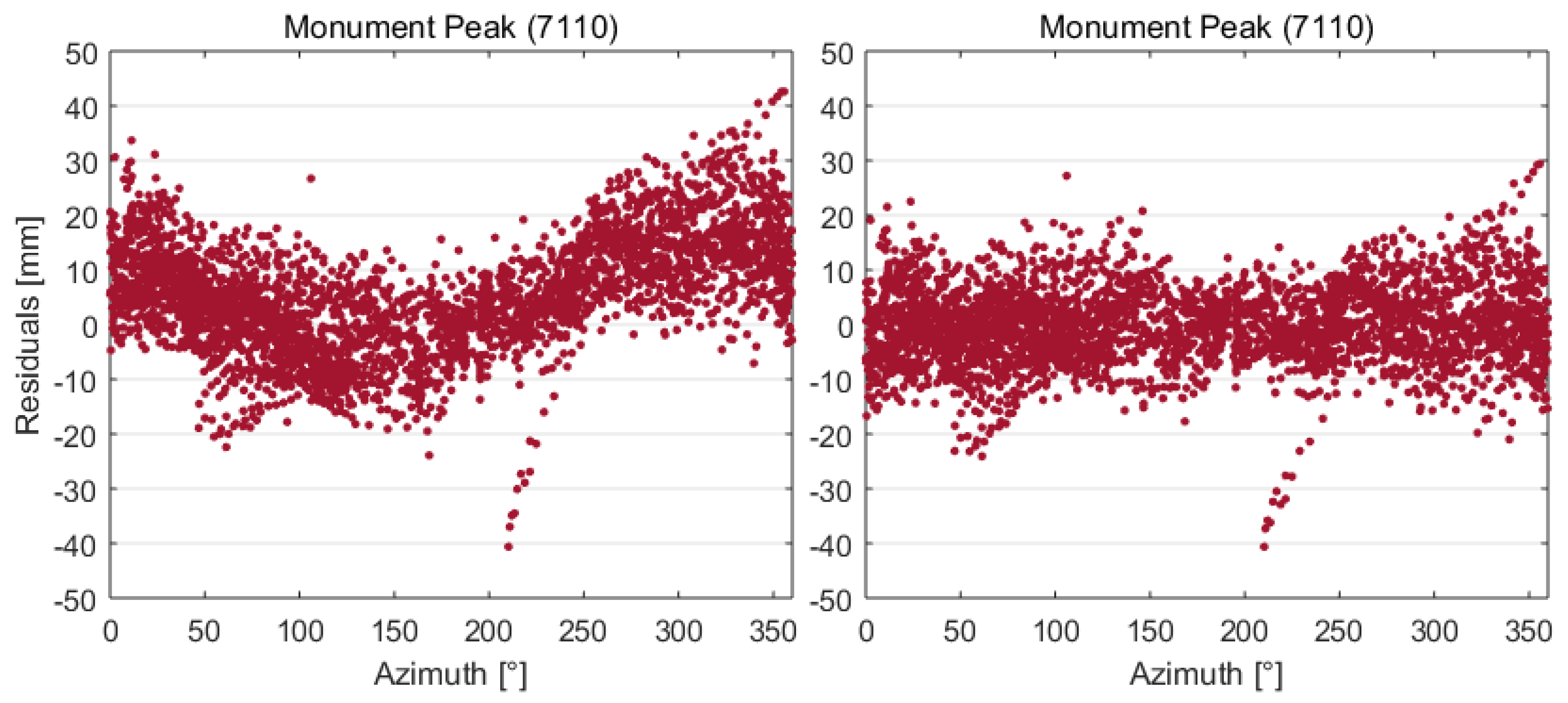
Figure 4.
Residual dependency on Monument Peak station azimuth angles for solutions with uncorrected (left) and corrected (right) range biases.
Figure 4.
Residual dependency on Monument Peak station azimuth angles for solutions with uncorrected (left) and corrected (right) range biases.
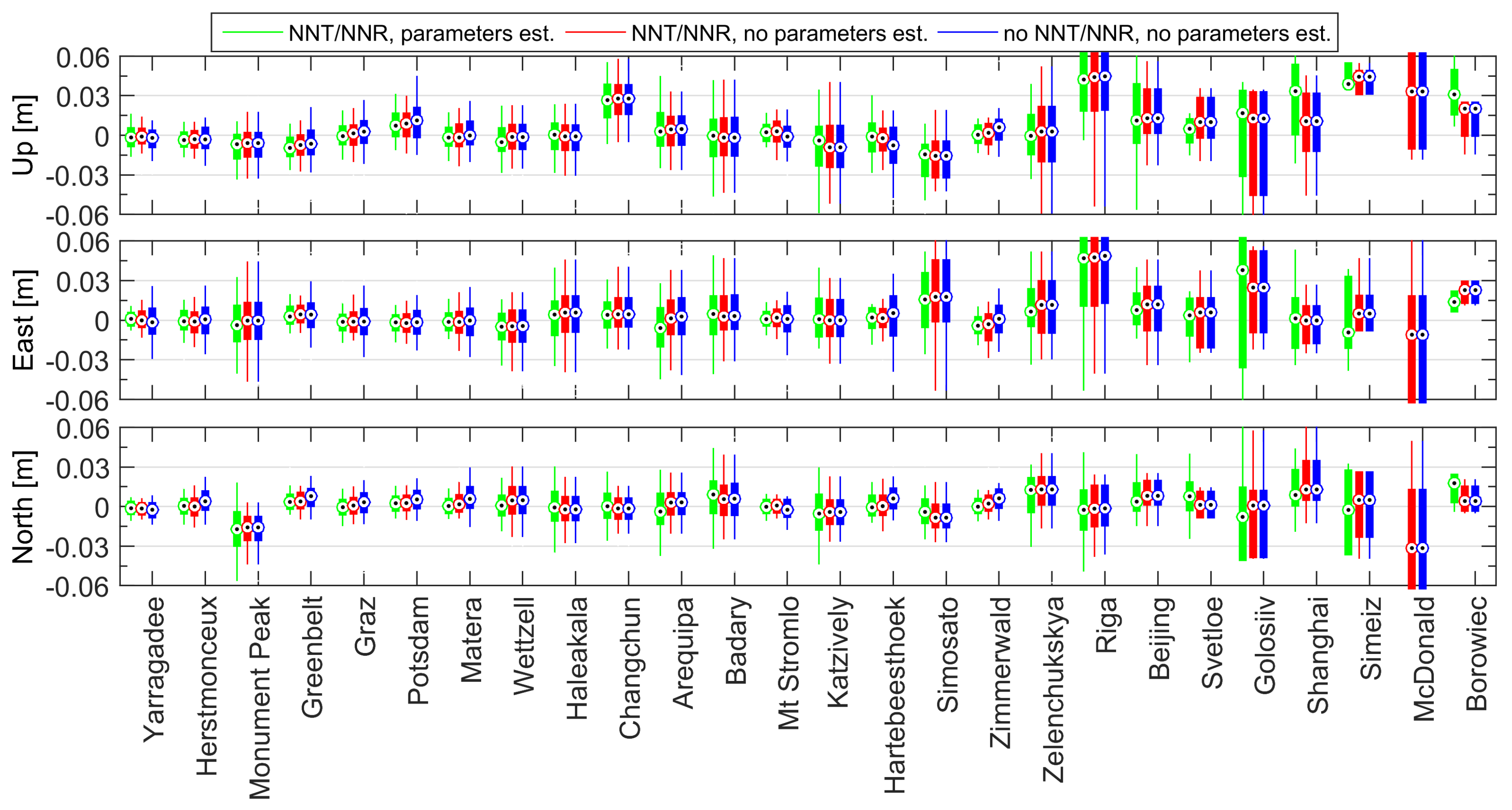
Figure 5.
SLR site coordinate repeatabilities in SLRF2014 based on SLR-to-S3A/B data for scenario 1 (green), scenario 2 (red), scenario 3 (blue). Minimum, maximum, 1st and 3rd quartiles and the median value are shown as elements of box-plots. Stations are sorted starting from that with the highest number of 7-day solutions (left) to the lowest number of solutions (right).
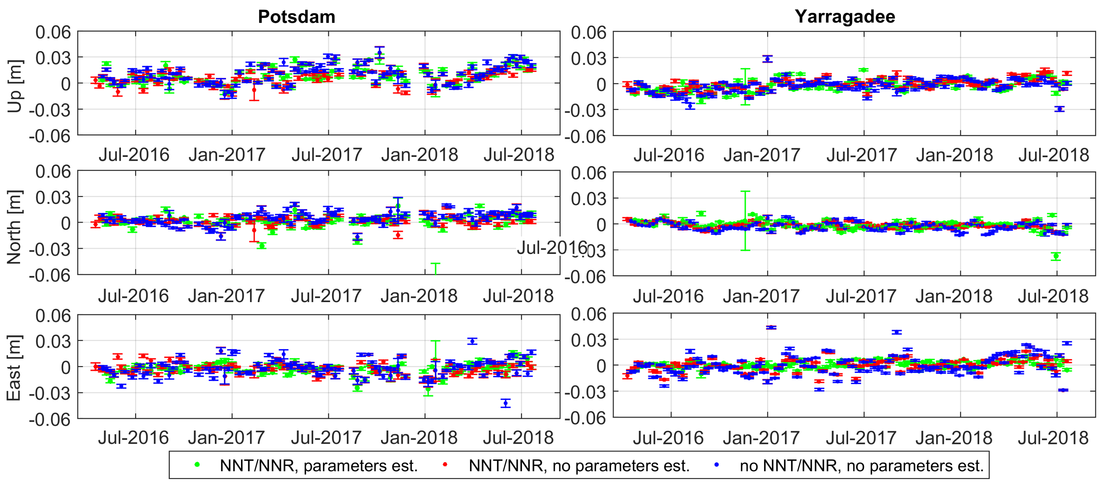
Figure 6.
Time series (with error bars) of estimated station coordinates for Potsdam (left) and Yarragadee (right) using SLR observations to S3A/B w.r.t a priori SLRF2014 coordinates for scenario 1 (green), 2 (red), 3 (blue).
Figure 6.
Time series (with error bars) of estimated station coordinates for Potsdam (left) and Yarragadee (right) using SLR observations to S3A/B w.r.t a priori SLRF2014 coordinates for scenario 1 (green), 2 (red), 3 (blue).
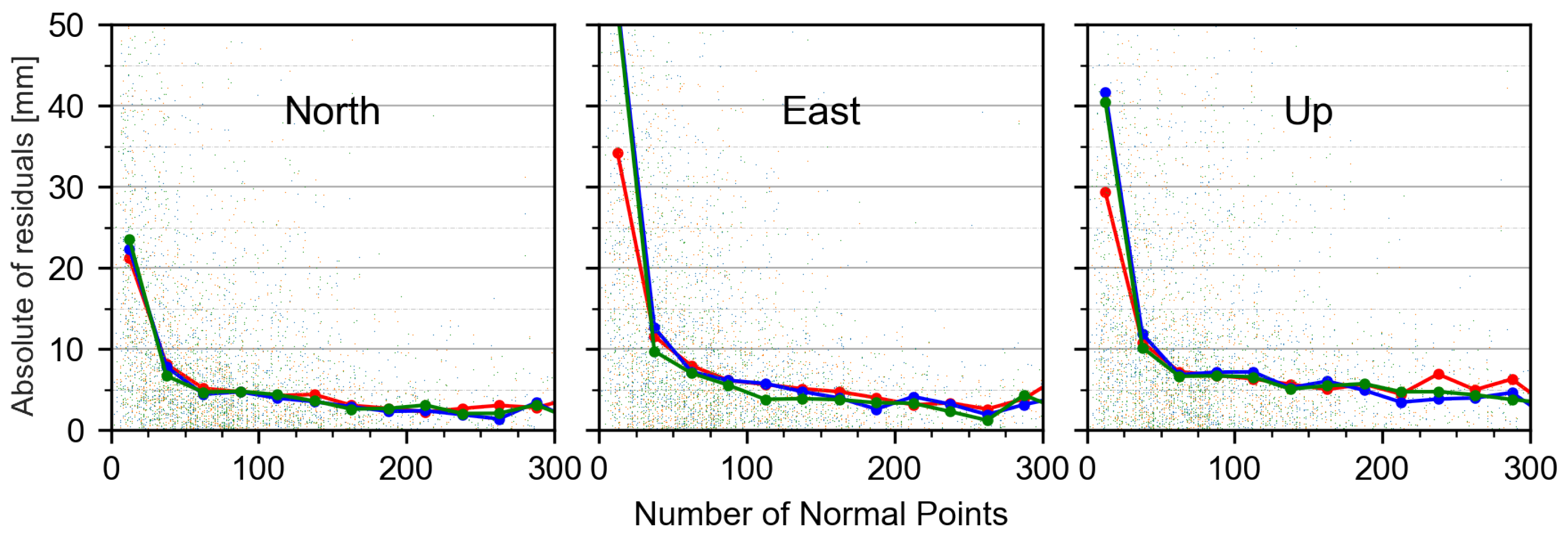
Figure 7.
Absolute of residuals of estimated SLR station coordinates based on S3A/B data referred to the a priori values from SLRF2014 as the function of the number of observations collected by all SLR stations for scenario 1 (green), 2 (red), 3 (blue).
Figure 7.
Absolute of residuals of estimated SLR station coordinates based on S3A/B data referred to the a priori values from SLRF2014 as the function of the number of observations collected by all SLR stations for scenario 1 (green), 2 (red), 3 (blue).
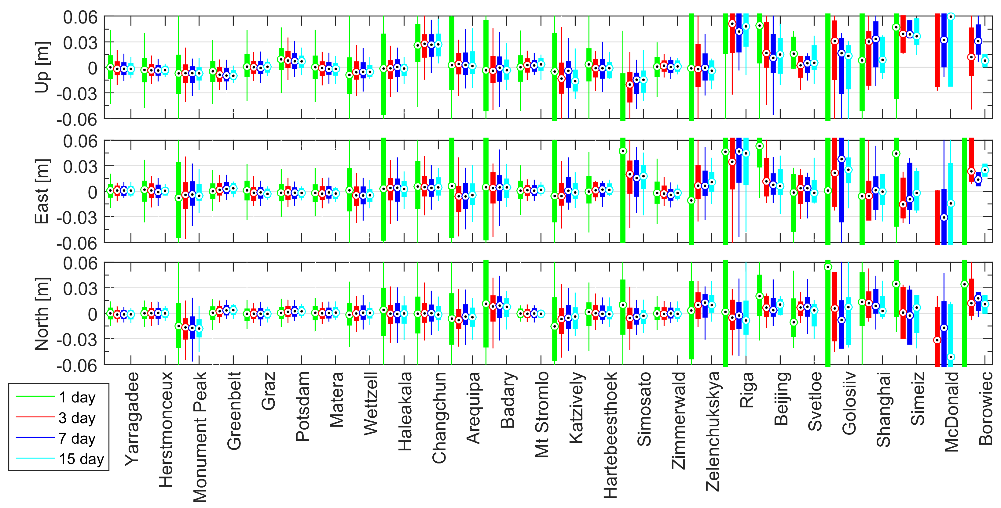
Figure 8.
Coordinate comparison to SLR2014 results from S3A/B when using different numbers of 1-day normal equations: 1-day (green), 3-day (red), 7-day (blue), 15-day (cyan). Minimum, maximum, 1st and 3rd quartiles and the median value are shown as elements of box-plots. Stations are sorted according to the number of 7-day solutions, starting with the highest number (left) to the lowest number of solutions (right).
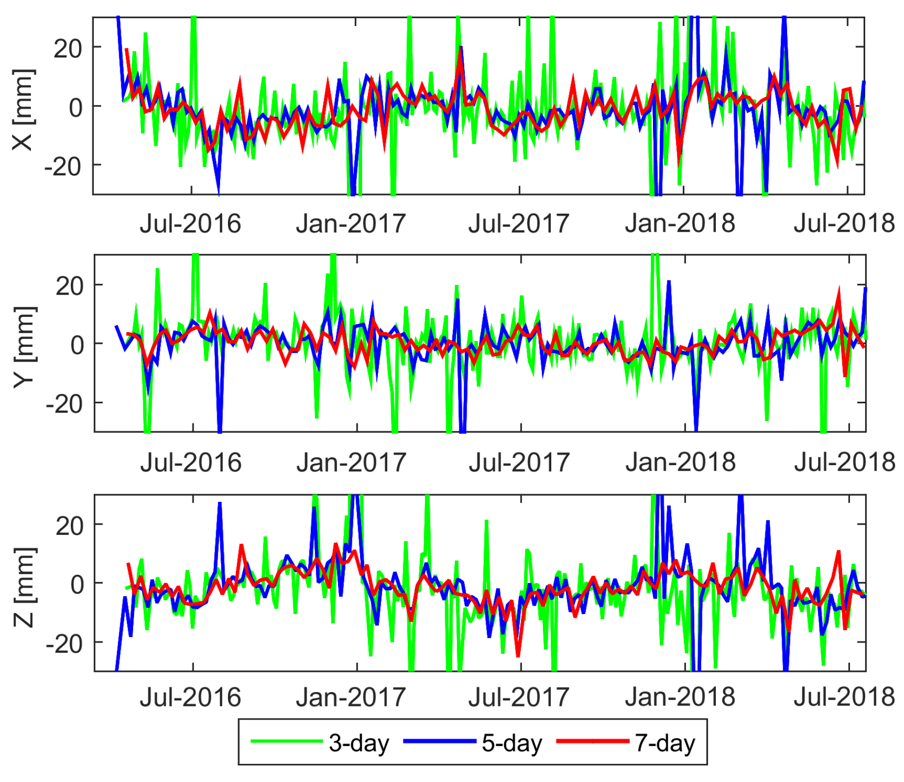
Figure 9.
Geocenter coordinates based on SLR observations to S3A/B from 3-day (green), 5-day (blue), 7-day (red) solutions all of which are based on stacking a different number of 1-day orbit solutions.
Figure 9.
Geocenter coordinates based on SLR observations to S3A/B from 3-day (green), 5-day (blue), 7-day (red) solutions all of which are based on stacking a different number of 1-day orbit solutions.
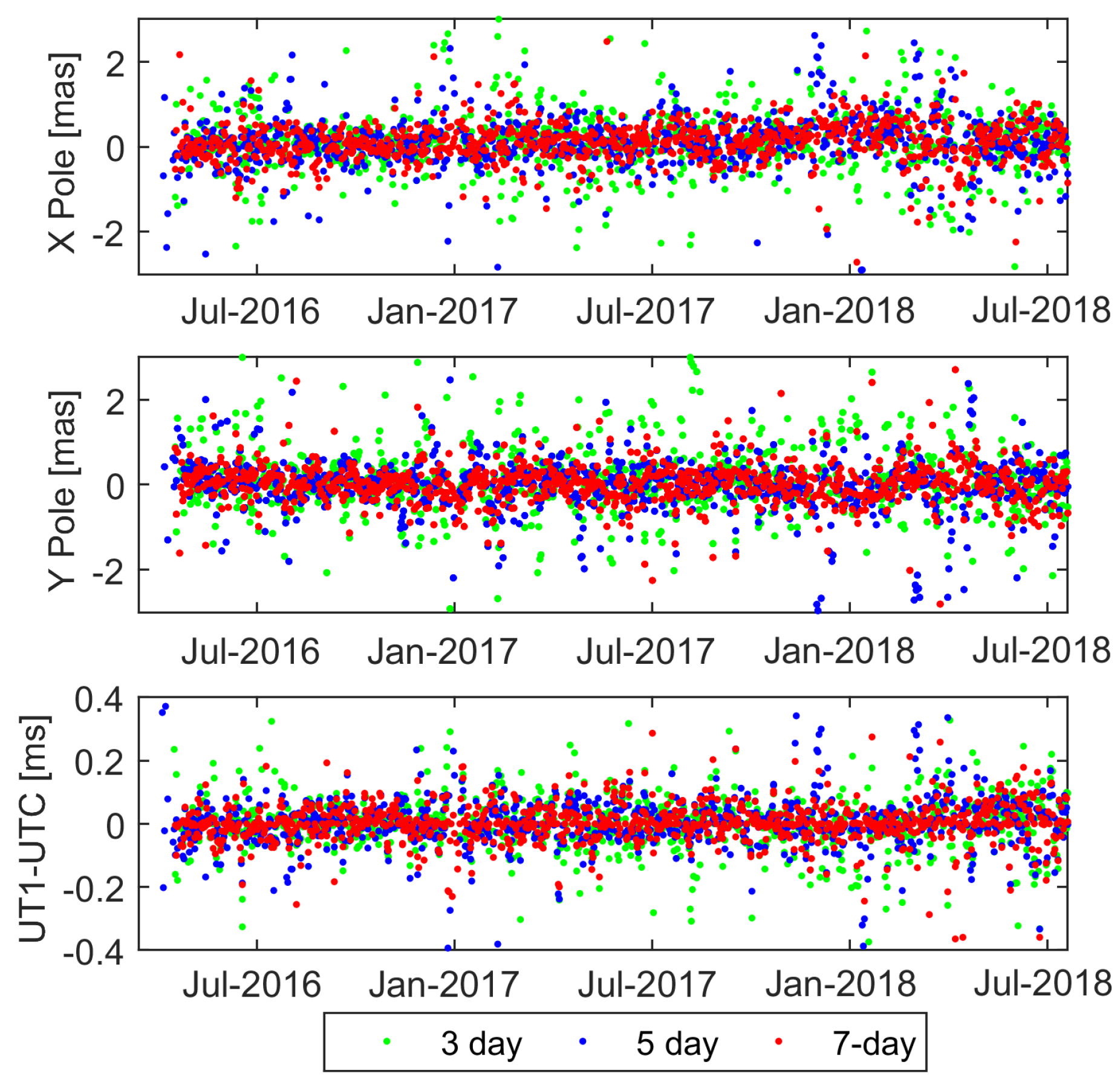
Figure 10.
Pole coordinates and the UT1-UTC from S3A/B w.r.t the IERS-14-C04 series for the tests using 3-day (green), 5-day (blue), and 7-day (red) solutions.
Figure 10.
Pole coordinates and the UT1-UTC from S3A/B w.r.t the IERS-14-C04 series for the tests using 3-day (green), 5-day (blue), and 7-day (red) solutions.
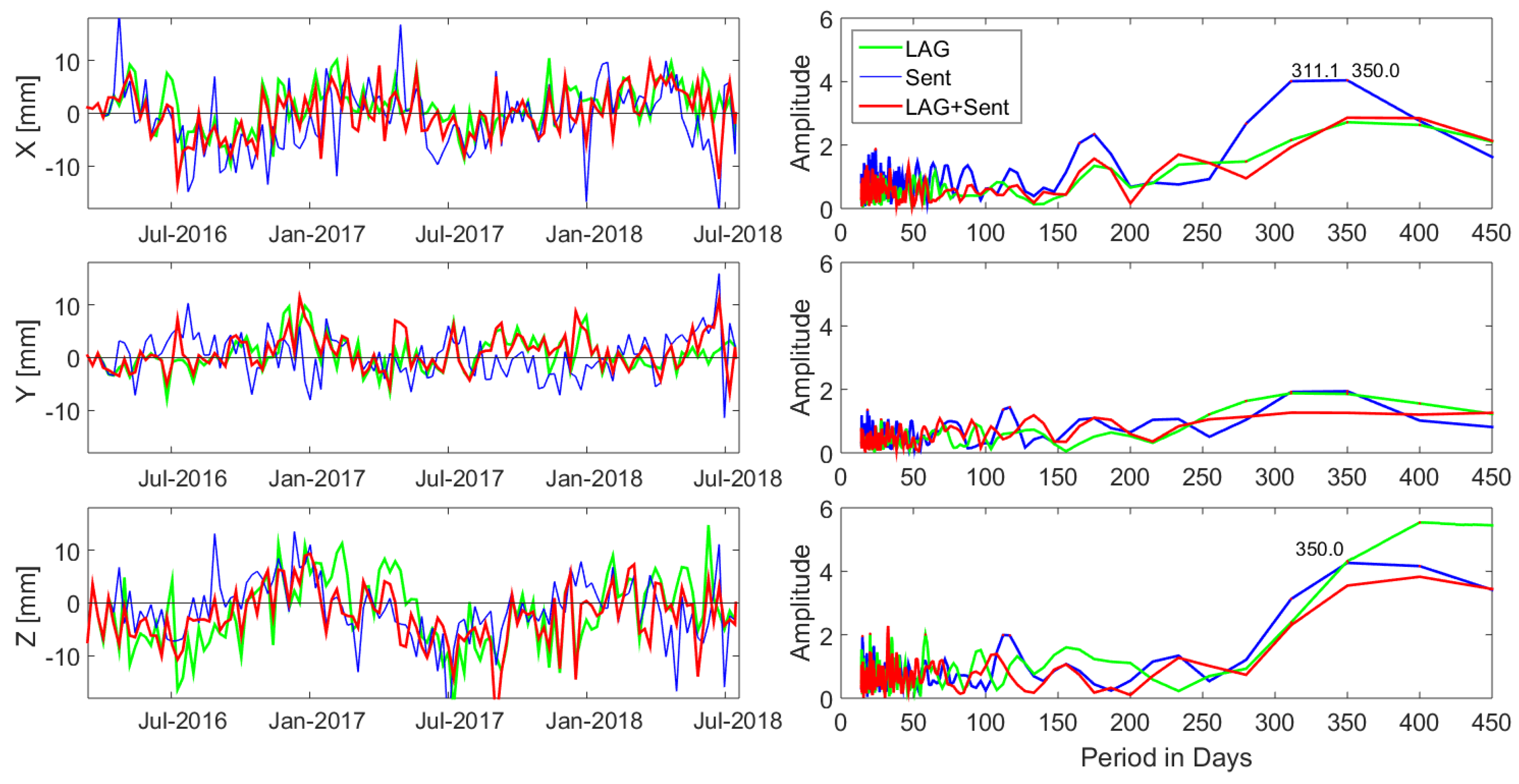
Figure 11.
Comparison of geocenter coordinates (left) and the spectral analysis (right) for LAG (green), Sent (blue), and LAG+Sent (red) solutions.
Figure 11.
Comparison of geocenter coordinates (left) and the spectral analysis (right) for LAG (green), Sent (blue), and LAG+Sent (red) solutions.
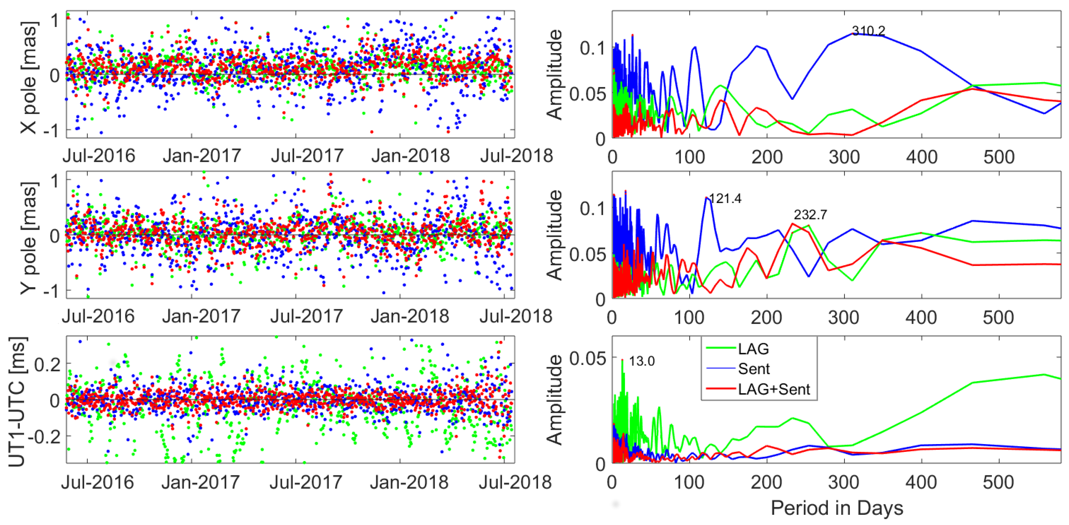
Figure 12.
Differences of pole coordinates and UT1-UTC w.r.t. IERS-14-C04 series and the spectral analysis of differences for LAG (green), Sent (blue), and LAG+Sent (red) solutions.
Figure 12.
Differences of pole coordinates and UT1-UTC w.r.t. IERS-14-C04 series and the spectral analysis of differences for LAG (green), Sent (blue), and LAG+Sent (red) solutions.
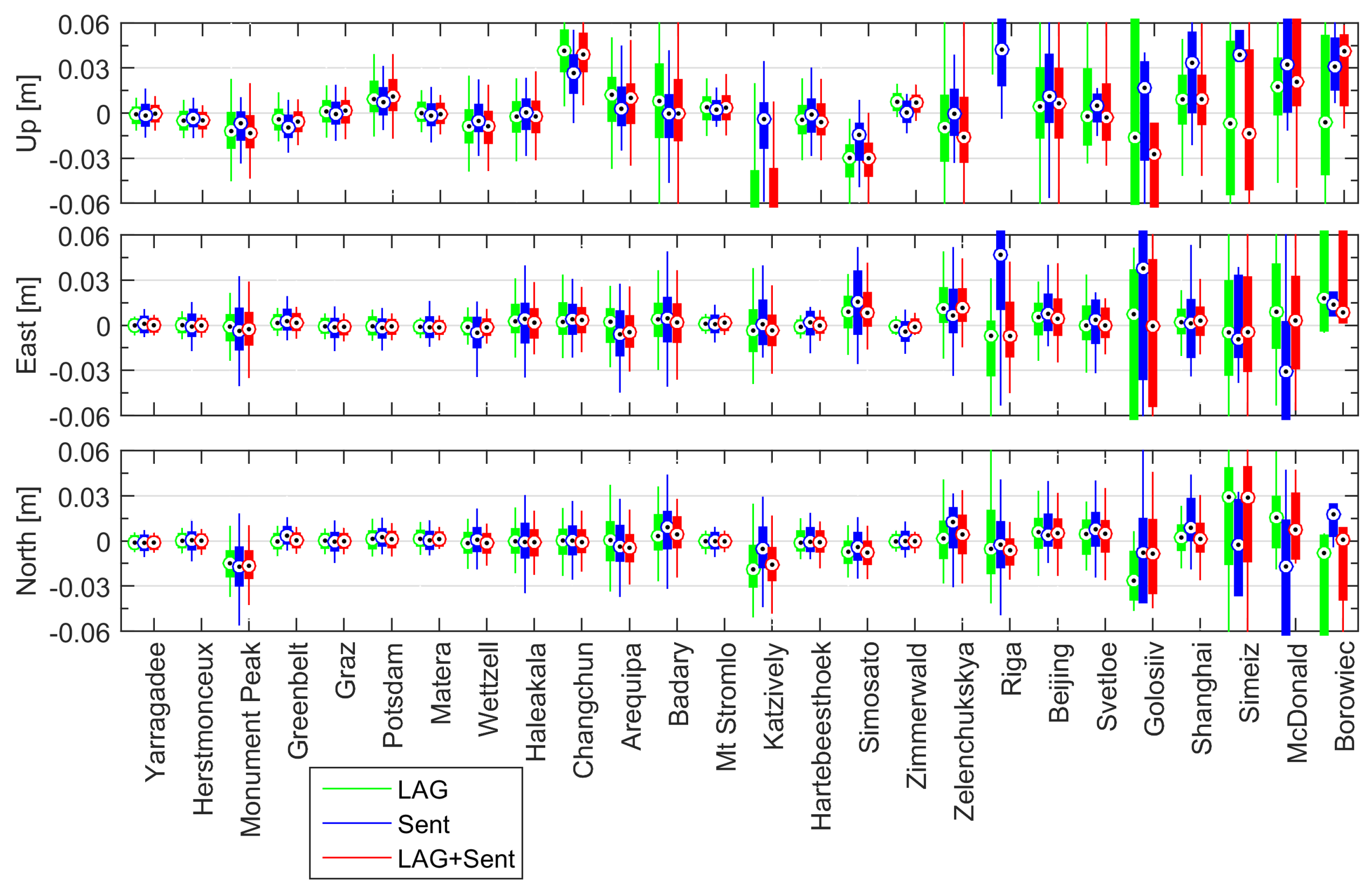
Figure 13.
Differences of estimated SLR station coordinates w.r.t. SLR2014 for LAG (green), Sent (blue), and LAG+Sent (red) solutions represented as box-plots with max., min., 1st, 3rd quartiles, and median values.
Figure 13.
Differences of estimated SLR station coordinates w.r.t. SLR2014 for LAG (green), Sent (blue), and LAG+Sent (red) solutions represented as box-plots with max., min., 1st, 3rd quartiles, and median values.
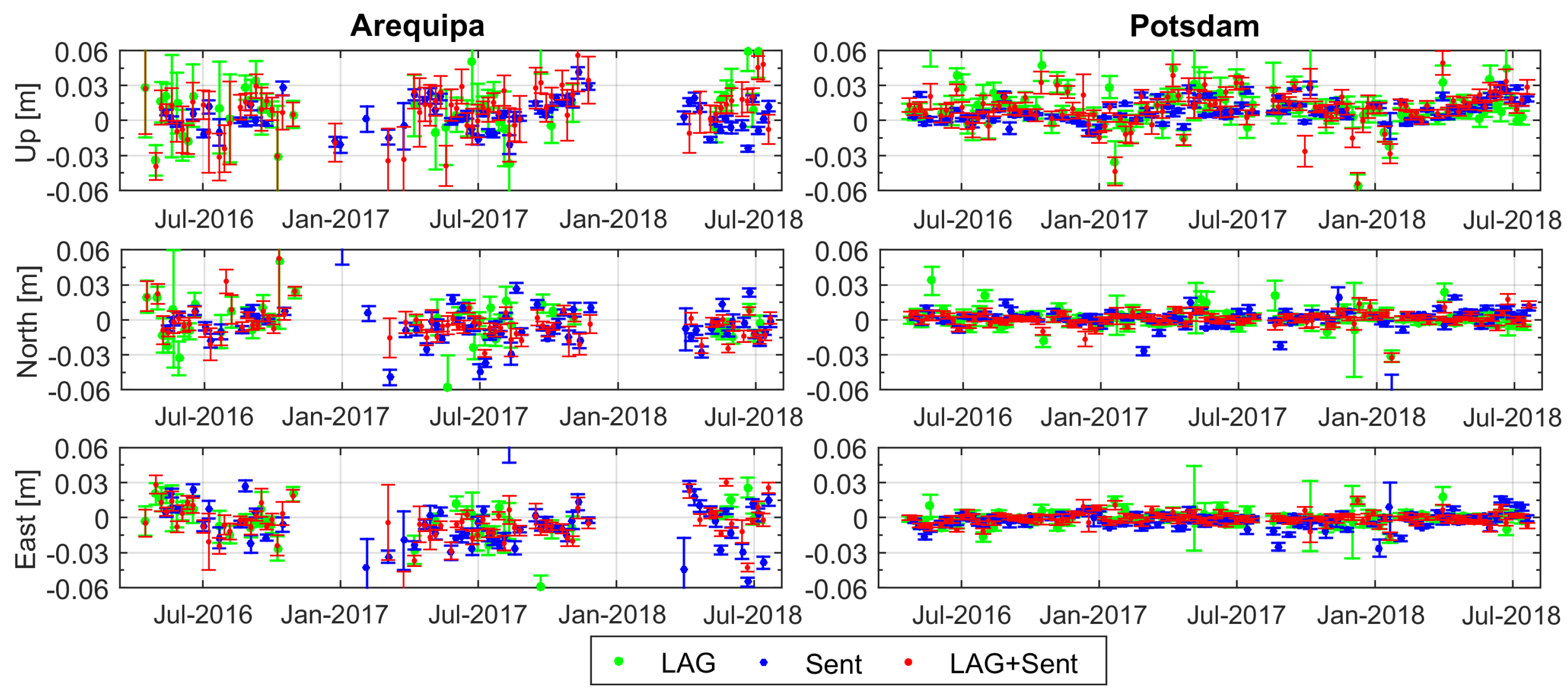
Figure 14.
Time series (error bars) for Arequipa (left) and Potsdam (right) site coordinates w.r.t SLRF2014 for LAG (green), Sent (blue), LAG+Sent (red) solutions.
Figure 14.
Time series (error bars) for Arequipa (left) and Potsdam (right) site coordinates w.r.t SLRF2014 for LAG (green), Sent (blue), LAG+Sent (red) solutions.
Table 1.
Constraints in tests of different network realization scenarios and different sets of estimated global parameters for S3A/B and LAG.
Table 1.
Constraints in tests of different network realization scenarios and different sets of estimated global parameters for S3A/B and LAG.
| 1cSolution Scenario | Network and Parameter Constraints |
|---|
| NNT [m] | NNR [rad] | Scale [mm] | Geocenter crd [m] | UT1-UTC [ms] | Pole Crds [µas] | Range Bias [m] |
|---|
| 1. NNT/NNR parameters est. | | | - | - | 2 | 30 | |
| 2. NNT/NNR no parameters est. | | | - | | | | |
| 3. no NNT/NNR no parameters est. | - | - | - | | | | |
| LAGEOS | | | - | | | | - |
Table 2.
SLR station coordinate repeatability for the North, East, and Up components for tested S3A/B solutions for all and top SLR sites (in mm).
Table 2.
SLR station coordinate repeatability for the North, East, and Up components for tested S3A/B solutions for all and top SLR sites (in mm).
| Sites | Solution Scenario | North | East | Up |
|---|
| Median | IQR | Median | IQR | Median | IQR |
|---|
| All sites | 1. NNT/NNR, all parameters est. | 0.0 | 11.7 | 0.2 | 13.4 | -0.8 | 16.3 |
| 2. NNT/NNR, no global par. est. | 0.3 | 11.5 | 1.1 | 15.2 | −0.3 | 16.9 |
| 3. no NNT/NNR, no global par. est. | 1.7 | 14.4 | 1.4 | 19.8 | 0.0 | 18.3 |
| Top sites | 1. NNT/NNR, all parameters est. | 0.5 | 7.8 | −0.4 | 9.1 | −1.6 | 11.9 |
| 2. NNT/NNR, no global par. est. | 1.1 | 8.5 | 0.2 | 11.4 | −0.6 | 12.3 |
| 3. no NNT/NNR, no global par. est. | 3.2 | 11.6 | 0.4 | 16.9 | −0.7 | 13.4 |
Table 3.
Mean offsets and RMS values of the estimated X, Y, Z geocenter coordinates (in mm). The mean values are calculated with respect to the ITRF2014/SLRF2014.
Table 3.
Mean offsets and RMS values of the estimated X, Y, Z geocenter coordinates (in mm). The mean values are calculated with respect to the ITRF2014/SLRF2014.
| Solution | X | Y | Z |
|---|
| Mean | RMS | Mean | RMS | Mean | RMS |
|---|
| LAG | 1.0 | 4.3 | 0.5 | 3.1 | −1.6 | 6.8 |
| Sent | −1.0 | 6.2 | 0.3 | 4.0 | −1.2 | 6.0 |
| LAG+Sent | 0.0 | 4.5 | 0.9 | 3.4 | −2.3 | 5.9 |
Table 4.
Mean offsets and RMS values of the estimated X, Y pole coordinates (in mas) and UT1-UTC (in ms) in reference to the a priori IERS-CO4-14 series.
Table 4.
Mean offsets and RMS values of the estimated X, Y pole coordinates (in mas) and UT1-UTC (in ms) in reference to the a priori IERS-CO4-14 series.
| 1cSolution | X pole | Y pole | UT1-UTC |
|---|
| mean | RMS | mean | RMS | Mean | RMS |
|---|
| LAG | 0.128 | 0.134 | 0.047 | 0.166 | −0.098 | 0.107 |
| Sent | 0.109 | 0.320 | 0.040 | 0.314 | −0.002 | 0.063 |
| LAG+Sent | 0.134 | 0.138 | 0.044 | 0.189 | −0.011 | 0.067 |
Table 5.
Statistics of summarized station coordinate repeatability for 7-day LAG, Sent, and LAG+Sent solutions with all SLR sites and top performing SLR sites decomposed into the North, East, and Up components (in mm).
Table 5.
Statistics of summarized station coordinate repeatability for 7-day LAG, Sent, and LAG+Sent solutions with all SLR sites and top performing SLR sites decomposed into the North, East, and Up components (in mm).
| 2cSolution | North | East | Up |
|---|
| median | IQR | median | IQR | median | IQR |
|---|
| All sites | LAG | −0.9 | 12.7 | 0.5 | 11.1 | −0.8 | 24.6 |
| Sent | 0.0 | 11.7 | 0.2 | 13.4 | −0.8 | 16.3 |
| LAG+Sent | −1.0 | 12.4 | 0.3 | 11.4 | −1.3 | 26.3 |
| Top sites | LAG | −0.1 | 5.3 | 0.0 | 5.0 | −0.4 | 12.5 |
| Sent | 0.5 | 7.8 | −0.4 | 9.1 | −1.6 | 11.9 |
| LAG+Sent | −0.2 | 5.2 | −0.1 | 5.2 | −0.7 | 12.3 |

 ,
, 


