Fuzzy Markovian Bonus-Malus Systems in Non-Life Insurance

Abstract

Markov chains (MCs) are widely used to model a great deal of financial and actuarial problems. Likewise, they are also used in many other fields ranging from economics, management, agricultural sciences, engineering or informatics to medicine. This paper focuses on the use of MCs for the design of non-life bonus-malus systems (BMSs). It proposes quantifying the uncertainty of transition probabilities in BMSs by using fuzzy numbers (FNs). To do so, Fuzzy MCs (FMCs) as defined by Buckley and Eslami in 2002 are used, thus giving rise to the concept of Fuzzy BMSs (FBMSs). More concretely, we describe in detail the common BMS where the number of claims follows a Poisson distribution under the hypothesis that its characteristic parameter is not a real but a triangular FN (TFN). Moreover, we reflect on how to fit that parameter by using several fuzzy data analysis tools and discuss the goodness of triangular approximates to fuzzy transition probabilities, the fuzzy stationary state, and the fuzzy mean asymptotic premium. The use of FMCs in a BMS allows obtaining not only point estimates of all these variables, but also a structured set of their possible values whose reliability is given by means of a possibility measure. Although our analysis is circumscribed to non-life insurance, all of its findings can easily be extended to any of the abovementioned fields with slight modifications.

1. Introduction

1.1. Motivation

A bonus-malus system (BMS) is a common method for posteriori ratemaking in non-life insurance. It is based on partitioning the insurer’s portfolio into a finite number of classes: bonus and malus classes. A typical case is automobile third-party liability insurance [1]. In a BMS, policyholders do not have a fixed price for their contracts throughout periods (e.g., the mathematical expectation of claims value per period). Their membership into a concrete BMS class is reviewed each period according to the number of claims in the previous one. Claim-free years are rewarded by discounts or bonuses on a base-premium; at-fault accidents are penalized by surcharges called maluses. Some overviews on how BMS are applied in different countries can be found in [2,3,4].

Following [5], in most commercial BMSs, by knowing the insured’s class in the current period and fitting the statistical distribution for the number of claims per period, it is possible to determine the probabilities of the insured’s class in the next period. Therefore, these BMSs are Markovian. For that reason, the academic literature on BMSs uses extensively MCs for their modeling ([1,5,6,7,8,9,10,11]). Therefore, a key question in a BMS is fitting the value of the one-step transition probability matrix. Following [12,13], if full knowledge of the probabilities of this matrix is not available, they have to be estimated somehow with the uncertainty that any estimation procedure involves. Uncertainty may be due to randomness, hazard, vagueness, incomplete information, etc. In our paper, we consider that the claiming process is probabilistic, but the uncertainty about the parameter that governs this random behavior is captured by means of a fuzzy number (FN) and, as a consequence, fuzzy Markov chains (FMCs) will be used.

1.2. Novelties

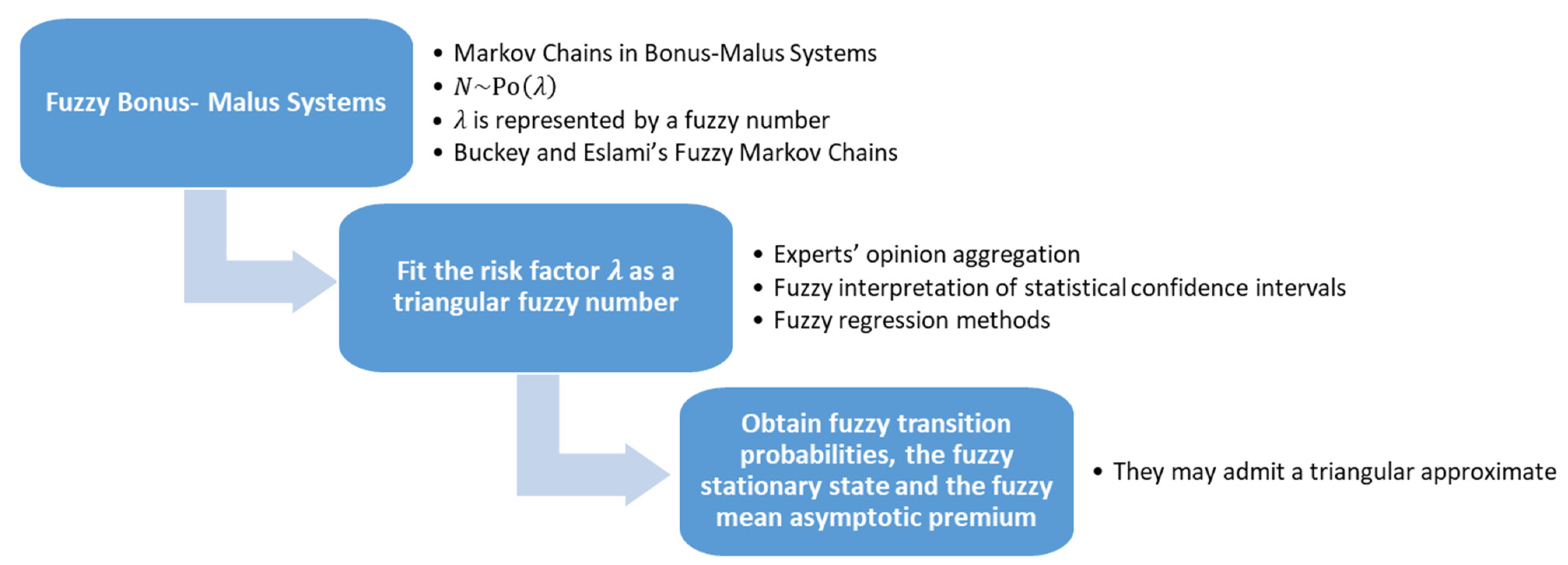
Although other hypotheses can be taken, such as, for example, considering that the number of claims in a period, N, follows a negative binomial distribution ([14]), academic literature on BMSs usually assumes that $N$ is a Poisson random variable (RV). So, $N~\mathrm{Po}\left(\lambda \right)$ and the parameter $\lambda$, the claim frequency, is perfectly known and can be interpreted as a risk measure of the policy. However, in a more realistic approach, some authors like [15] use intervals to quantify the uncertainty about the parameter of a distribution function that governs a risk variable. This is also the case within a BMS framework of [11], who model the uncertainty about $\lambda$ by means of a modal interval. One extended way to combine randomness and uncertainty of parameters of distribution functions consists in modeling these parameters as FNs. It has been done both for continuous RVs ([16,17,18]), and in the discrete case ([19]). Following this approach, [20,21] and also [15] model risk financial parameters with FNs. In the actuarial field, FNs have been used to capture the uncertainty of insurance pricing variables ([22]) but also to model parameters that quantify risks. In this regard, we can point out [23] in a non-life insurance context, [24] to interpret the parameter that quantifies the dependence in a Farlie-Gumbel-Morgestein copula, and [25,26,27,28] in life insurance pricing. Since any interval can be seen as the $\alpha$-cut of a FN, even in the case of improper intervals ([29]), in this work we consider that $\lambda$ is fitted by means of a FN and, more particularly, by a triangular fuzzy number (TFN). So, this paper builds up a framework to model Markovian BMSs that embed the standard case, where the risk parameter $\lambda$ is crisp, but also the method developed in [11] that quantifies this parameter as a modal interval. Standard BMSs provide point values for the stationary state and the mean asymptotic premium. Modal BMSs as introduced in [11] allow obtaining these variables as modal intervals whose lower and upper bounds may be understood as pessimistic/optimistic scenarios. Our method generalizes both types of BMSs since it quantifies variables related to BMS as FNs. On the one hand, these FNs can be understood as a set of crisp outcomes with an associated possibility measure. On the other, these FNs can be interpreted as a set of intervals that come from pessimistic/optimistic scenarios and are structured by means of possibility levels. Figure 1 shows a graphical synthesis of the methodological framework developed in this paper.

Other more complex forms of FNs, such as generalized FNs (GFNs) or intuitionistic FNs (IFNs), could be considered to quantify uncertain probabilities. Tools like GFNs or IFNs provide a more complete capture of uncertainty than FNs. However, their adjustment has a greater cost than in the case of triangular FNs since they incorporate more parameters and their computational handle may be more expensive as well. Therefore, using TFNs supposes a balance between the simplicity of crisp or modal interval probabilities and more complex representations of uncertain quantities such as GFNs or IFNs.

It should be noted that there are several scientific fields in which MCs are in use. In the field of economics and finance, we can observe applications within Leontief’s input-output model, credit risk measurement, asset price volatility modeling, life insurance, etc. In addition, MCs have shown their usefulness in many other areas: industrial engineering (e.g., queuing theory), computer science (e.g., computer performance evaluation and web search engines), healthcare (e.g., pandemics transmission or evolution of ICU patients), etc. Hence, although our developments are carried out within a non-life insurance context, most of the results can be applied to any problem modeled by means of MCs when the transition probabilities (or the parameters that define them) are not precisely known.

The paper is organized as follows. Section 2 describes briefly how BMSs work. Section 3 shows the basic concepts of FNs and FMCs used throughout the paper. In Section 4, a methodologic approach is proposed to fit a fuzzy BMS (FBMS) when the number of claims within a period, $N$, follows a Poisson distribution with fuzzy parameter $\lambda$. This methodology is applied to the Irish BMS. A sensitivity analysis is conducted in Section 5. Finally, in Section 6, the work ends with a summary of its main contributions and potential extensions.

2. Markovian Bonus-Malus Systems in Non-Life Insurance

A BMS is a usual way to deal with risk aversion and moral hazard in some types of insurance, e.g., automobile third-party liability insurance [1]. BMSs classify insureds in $r$ classes in such a way that the percentage of the base-premium to be paid by the $i$th class, $b_i$, satisfies $b_i<b_{i+1}$, $i=1,2,\dots ,r-1$. In a BMS, the transition between classes is governed by a set of rules defined over the insured’s number of claims in the current period. To summarize, it can be said that every BMS is determined by three elements (see

Table 1. Elements of a bonus-malus system (BMS).

Class	Premium Level	Class after $\mathit{k}$ Claims
$\mathit{i}$	${\mathit{b}}_{\mathit{i}}$	$\mathit{k}=\mathbf{0}$	$\mathit{k}=\mathbf{1}$	…	$\mathit{k}\ge \mathit{n}$
$r$	$b_r$
$⋮$	$⋮$
$i_0$	$b_{i_0}$
$⋮$	$⋮$
1	$b_1$

Source: Own elaboration based on [10].

):

• The initial class, where new insureds are assigned, $i_0$.
• The premium scale $b=\left(b_1,\dots ,b_r\right)$.
• The transition rules, that is to say, the rules that define the conditions for an insured in one class to be transferred to another class in the next period.

Let us model the insured’s class at time $t$ as a discrete stochastic process ${\left(X_t\right)}_{t\in \mathbb{N}}$, being its state space the classes $S=\left\{1,2,\dots ,r\right\}\subset \mathbb{N}$. Furthermore, as it is usually done in the literature (e.g., [10]), we consider that the BMS is a finite MC, i.e., $p\left(X_{n+1}=i_{n+1}|X_0=i_0,X_1=i_1,\dots ,X_n=i_n\right)=p\left(X_{n+1}=i_{n+1}|X_n=i_n\right)$, $\forall i_0,i_1,\dots ,i_{n+1}\in S$. An insurer uses a finite Markovian BMS when the following conditions hold [1]:

• There exists a finite number of classes such that each insured stays in one class through each period.
• The premium for each insured depends only on the class where they stay.
• The class for a given period is determined by the class in the preceding period and the number of claims reported in that period.

A finite MC is said to be homogeneous if $p\left(X_{m+h}=j|X_m=i\right)$ does not depend on $m$. In this case, transition probabilities $p_{ij}=p\left(X_{t+1}=j|X_t=i\right)$, i.e., probabilities of moving from class $i$ to class $j$ in one-step (period), can be collected in a transition matrix $P=\left(p_{ij}\right)$ with order $r$. The elements $p_{ij}$ satisfy $p_{ij}\ge 0$ and ${\displaystyle \sum }_{j=1}^r{p}_{ij}$ = 1.

If ${\left(p_i^{\left(0\right)}\right)}_{i\in S}$ denote the probabilities of initially being in state $i\in S$, the probabilities of being in state $i\in S$ after $n$ periods, ${\left(p_i^{\left(n\right)}\right)}_{i\in S}$ are:

$$p_i^{\left(n\right)}=p_i^{\left(n-1\right)}·P=p_i^{\left(n-2\right)}·P·P=\dots =p_i^{\left(0\right)}·P^n$$

(1)

where $P^n$ is represented by $P^{\left(n\right)}=\left(p_{ij}^{\left(n\right)}\right)$ and $p_{ij}^{\left(n\right)}$ are the probabilities of moving from state $i$ to state $j$ in $n$ period. From Equation (1), it follows that:

$$p_{ij}^{\left(n\right)}=f_{ij}^{\left(n\right)}\left(p_{11},\dots ,p_{1r},p_{21},\dots ,p_{2r},\dots ,p_{1r},\dots ,p_{rr}\right)$$

(2)

for some continuous functions $f_{ij}^{\left(n\right)}$, i.e., the elements in $P^n$ are some functions of the elements in $P$.

A homogeneous MC is regular if each state is accessible from any other state, either in one step or more, i.e., there exists $n\in \mathbb{N}$ such that $p_{ij}^{\left(n\right)}>0$ $\forall i,j$. One of the features that characterize regular MCs is its stationary distribution, which represents the probability of the chain being at each state after a large number of periods, namely, $\underset{n\to \infty }{\lim }{P}^n=\pi$, where the rows of $\pi$ are identical. So, any regular MC with transition matrix $P$ has a stationary distribution, $\pi$, such that:

$$\pi =\pi ·P$$

(3)

The vector $\pi ={\left({\pi }_j\right)}_{j=1,2,\dots ,r}$ can be interpreted as the probability that an insured belongs to class $j,$ $j=1,2,\dots ,r$ after $n$ periods, $n\to \infty$. That vector does not depend on the insured’s initial class, $i_0$. So, two main outputs in a BMS are:

• The stationary distribution of $X_t$, $\pi$, as defined in Equation (3).
• The mean asymptotic premium, $b^{*}$, i.e., the average premium paid by the insured in that stationary distribution, defined as:

  $$b^{*}={\displaystyle \sum }_{j=1}^r{b}_j{\pi }_j$$

  (4)

The mean asymptotic premium, $b^{*}$ is a concept of the utmost importance because it has been intensively used to assess the efficiency of a BMS (e.g., [1,6,30,31]).

BMSs consider the number of claims, $N$, as a discrete RV. In our paper, as it is commonplace in actuarial literature, $N$ is supposed to follow a Poisson distribution with parameter $\lambda$, $N~\mathrm{Po}\left(\lambda \right),$ ([1,7,8,9,10,11,12]). Therefore:

$$p\left(N=k\right)=\frac{{\lambda }^k}{k!}{e}^{-\lambda }$$

(5)

where $p(·)$ stands for a probability measure.

Poisson RVs are often used in actuarial modeling due to their interesting arithmetical properties. Furthermore, the risk parameter $\lambda$ can be fitted specifically to each insured taking into account relevant rating factors (e.g., gender, age, and social status) by using a generalised linear model (GLM) ([5,8,32]).

If $N$ is modeled with (5), $p_{ij}$ is a function of the risk parameter $\lambda$, $h_{ij}\left(\lambda \right),$ in such a way that the BMS probabilities in the one-step transition matrix are:

$$h_{ij}\left(\lambda \right)=p_{ij}={\displaystyle \sum }_{k=0}^{\infty }\frac{{\lambda }^k}{k!}{e}^{-\lambda }{t}_{ij}\left(k\right)$$

(6)

where $t_{ij}\left(k\right)=1$ $\mathrm{if}k\mathrm{causes}\mathrm{the}\mathrm{transition}\mathrm{from}i\mathrm{to}j$ and 0 otherwise.

Numerical application 1. Let $\lambda =0.04$ in Equation (5) for the Irish BMS in

Table 2. Irish bonus-malus system.

Class	Premium Level	Class after $\mathit{k}$ Claims
$\mathit{i}$	${\mathit{b}}_{\mathit{i}}$	$\mathit{k}=\mathbf{0}$	$\mathit{k}=\mathbf{1}$	$\mathit{k}\ge \mathbf{2}$
6	100	5	6	6
5	90	4	6	6
4	80	3	6	6
3	70	2	5	6
2	60	1	4	6
1	50	1	3	6

Source: [10].

. The transition matrix, $P$, that corresponds to this BMS is:

$$\left(\begin{array}{cccccc}p\left(N=0\right)& 0& p\left(N=1\right)& 0& 0& p\left(N\ge 2\right)\\ p\left(N=0\right)& 0& 0& p\left(N=1\right)& 0& p\left(N\ge 2\right)\\ 0& p\left(N=0\right)& 0& 0& p\left(N=1\right)& p\left(N\ge 2\right)\\ 0& 0& p\left(N=0\right)& 0& 0& p\left(N\ge 1\right)\\ 0& 0& 0& p\left(N=0\right)& 0& p\left(N\ge 1\right)\\ 0& 0& 0& 0& p\left(N=0\right)& p\left(N\ge 1\right)\end{array}\right)$$

(7)

From (3), $\pi =\left(0.916232,0.037394,0.038921,0.003861,0.002523,0.001069\right)$ and, by considering Equation (4), the mean asymptotic premium is $b^{*}=51.423$.

In this paper, we will consider that the risk parameter $\lambda$ cannot be determined precisely. Uncertainty may be the result of different causes: stochastic variability, inaccuracy, incomplete information, etc. Stochastic variability can be described by using RVs or stochastic processes, but inaccuracy and incomplete information can be captured by means of intervals or FNs. Given that any interval can be interpreted as the $\alpha$-cut of a FN, in this work it is assumed that $\lambda$ is a FN.

3. Fuzzy Numbers and Fuzzy Markov Chains

3.1. Fuzzy Numbers

A fuzzy number is a fuzzy set $\tilde{A}$ on the referential set $\mathbb{R}$ that satisfies (i) $\tilde{A}$ is normal, (ii) $\tilde{A}$ is convex, and (iii) the $\alpha$-cuts of $\tilde{A}$, $A\left(\alpha \right)=\left[\underset{\_}{A}\left(\alpha \right),\overline{A}\left(\alpha \right)\right],$ are closed and bounded (compact) intervals $\forall \alpha \in \left[0,1\right]$. The lower and upper bounds of the FN $A\left(\alpha \right)$ are:

$$A\left(\alpha \right)=\left[\underset{\_}{A}\left(\alpha \right),\overline{A}\left(\alpha \right)\right]=\left[\underset{x\in \mathbb{R}}{\inf }\left\{{\mu }_{\tilde{A}}\left(x\right)\ge \alpha \right\},\underset{x\in \mathbb{R}}{\sup }\left\{{\mu }_{\tilde{A}}\left(x\right)\ge \alpha \right\}\right]$$

(8)

FNs can be interpreted as the extension of the concept of a real number.

A triangular fuzzy number represented as $\tilde{A}=\left(A_L/A_C/A_U\right)$, is a FN whose $\alpha$-cuts, $\forall \alpha \in \left[0,1\right],$ are, from Equation (8):

$$A\left(\alpha \right)=\left[\underset{\_}{A}\left(\alpha \right),\overline{A}\left(\alpha \right)\right]=\left[A_L+\left(A_C-A_L\right)\alpha ,A_U-\left(A_U-A_C\right)\alpha \right]$$

(9)

from where, if needed, the membership of $\tilde{A}$ could be obtained. The core of $\tilde{A}$ is $A_C$ and can be understood as the most reliable value of this TFN. i.e., the possibility of $A_C$ is 1. The support of $\tilde{A}$ is $\left[A_L,A_U\right]$. TFNs are used in countless practical applications including actuarial ones [22] because they are easy to handle arithmetically and they are well adapted to the way humans think of uncertain quantities. Moreover, when the information about a variable is vague and imprecise, the parsimony principle leads us to represent that information as simply as possible. The linear shape of TFNs meets that requirement. For instance, the uncertain quantity “approximately $0.04$” can be represented in a very natural way as the TFN $\left(0.038/0.04/0.042\right)$.

Likewise, let it be a TFN $\tilde{A}$:

$$\tilde{A}>x(\mathrm{or}\ge x)\mathrm{if}{A}_L>x(A_L\ge x)\forall x\in \mathbb{R}$$

(10)

$$\tilde{A}<x(\mathrm{or}\le x)\mathrm{if}{A}_U<x(A_L\le x)\forall x\in \mathbb{R}$$

(11)

Let $f$ be a continuous real-valued function of $n$-real variables $x=\left(x_1,x_2,\dots ,x_n\right)$, $f\left(x\right)=f\left(x_1,x_2,\dots ,x_n\right)$. If $x_{j}s$ are not crisp numbers, but FNs ${\tilde{A}}_j$ with $\alpha$–cuts $A_j\left(\alpha \right)=\left[{\underset{\_}{A}}_j\left(\alpha \right),{\overline{A}}_j\left(\alpha \right)\right]$, $j=1,2,\dots ,n$, a FN $\tilde{B}$ is induced via $f$ such that $\tilde{B}=f\left({\tilde{A}}_1,{\tilde{A}}_2,\dots ,{\tilde{A}}_n\right)$. It is often difficult to obtain a closed expression for the membership function of $\tilde{B}$. However, following [33], the $\alpha$-cuts of $\tilde{B}$, $B\left(\alpha \right)$, in the usual case where $A_1\left(\alpha \right),\dots ,A_n\left(\alpha \right)$ are not interactive, i.e., the variables that they quantify have an independent behavior, can be obtained as:

$$B\left(\alpha \right)=\left\{f\left(x\right)|x=\left(x_1,x_2,\dots ,x_n\right)\in Dom\left(\alpha \right)\right\}$$

(12)

where $Dom\left(\alpha \right)$ stands for the rectangular domain:

$$Dom\left(\alpha \right)=\left\{x_j\in \left[{\underset{\_}{A}}_j\left(\alpha \right),{\overline{A}}_j\left(\alpha \right)\right],j=1,2,\dots ,n\right\}$$

(13)

So, the lower (upper) bounds of $B\left(\alpha \right)$, $\underset{\_}{B}\left(\alpha \right)$ ($\overline{B}\left(\alpha \right)$), are the global minimum (maximum) of $f\left(x\right)$ within the rectangular domain in Equation (13), that is to say:

$$\underset{\_}{B}\left(\alpha \right)=\underset{j,k}{\min }\left\{f\left(V_j\right),f\left(E_k\right)\right\}\mathrm{and}\overline{B}\left(\alpha \right)=\underset{j,k}{\max }\left\{f\left(V_j\right),f\left(E_k\right)\right\}$$

(14)

being $V_j$, $j=1,2,\dots ,2^n$, a vertex of the domain (13) and $f\left(E_k\right)$, $k=1,2,\dots ,K$, an extreme value of the function $f$ within this domain that takes this value at point $x=E_k$.

Therefore, if $f\left(x_1,x_2,\dots ,x_n\right)$ is monotonic, the lower and upper bounds of $B\left(\alpha \right)$, $\underset{\_}{B}\left(\alpha \right)$ and $\overline{B}\left(\alpha \right)$, are in one of the $2^n$ vertexes of (13). Without loss of generality, let us suppose that $f$ increases with respect to $x_j,j=1,2,\dots ,m$, $m\le n$, and decreases in the last $n-m$ variables, [34] demonstrates that:

$$(B\left(\alpha \right)=\left[\underset{\_}{B}\left(\alpha \right),\overline{B}\left(\alpha \right)\right]=[f\left({\underset{\_}{A}}_1\left(\alpha \right),{\underset{\_}{A}}_2\left(\alpha \right),\dots ,{\underset{\_}{A}}_m\left(\alpha \right),{\overline{A}}_{m+1}\left(\alpha \right),{\overline{A}}_{m+2}\left(\alpha \right),\dots {\overline{A}}_n\left(\alpha \right)\right),$$

(15)

$$f\left({\overline{A}}_1\left(\alpha \right),{\overline{A}}_2\left(\alpha \right),\dots {\overline{A}}_m\left(\alpha \right),{\underset{\_}{A}}_{m+1}\left(\alpha \right),{\underset{\_}{A}}_{m+2}\left(\alpha \right),\dots ,{\underset{\_}{A}}_n\left(\alpha \right)\right)]$$

If $A_1\left(\alpha \right),\dots ,A_n\left(\alpha \right)$ are interactive, (15) cannot be used to evaluate $B\left(\alpha \right)$. However, according to [35], the general formulation to obtain the lower and upper bounds of $B\left(\alpha \right)$ from Equations (12)–(14) is still valid but now the number of vertexes, $j$, is less than $2^n$. In [35], the authors study the role of interactive fuzzy variables in decision-making problems and analyze some particular cases. Concretely, when $f\left(x\right)$ is the mathematical expectation function, $x_j$ is the probability of the $j$th outcome, and it is quantified as a FN, the domain in Equation (13) turns into:

$$Dom\left(\alpha \right)=\left\{x_j\in \left[{\underset{\_}{A}}_j\left(\alpha \right),{\overline{A}}_j\left(\alpha \right)\right],{\displaystyle \sum }_{j=1}^n{x}_j=1\right\}$$

(16)

and Equation (14) becomes:

$$\underset{\_}{B}\left(\alpha \right)=\underset{j}{\min }\left\{f\left(V_j\right)\right\}\mathrm{and}\overline{B}\left(\alpha \right)=\underset{j}{\max }\left\{f\left(V_j\right)\right\}$$

(17)

due to the fact that $f\left(x\right)$ is a linear function.

It is worth noting that the result $\tilde{B}$ of evaluating a non-linear $f$ with the TFNs ${\tilde{A}}_j$ is not necessarily a TFN. However, often $\tilde{B}$ admits a good triangular approximation through the secant approach. It builds up the shape of the triangular approximate FN ${\tilde{B}}^{\prime }$ to $\tilde{B}$ by means of the secant lines that unite the 0-cut and the 1-cut of $\tilde{B}$. Such that ${\tilde{B}}^{\prime }$ is a TFN as:

$$\tilde{B}\approx {\tilde{B}}^{\prime }=\left(B_L/B_C/B_U\right)=\left(\underset{\_}{B}\left(0\right)/\underset{\_}{B}\left(1\right)=\overline{B}\left(1\right)/\overline{B}\left(0\right)\right)$$

(18)

This approximation, as shown in [36], works pretty well for nonlinear monotonic functions of TFNs such as product, division, power, etc. Likewise, [37,38] show that this approach fits satisfactorily common actuarial and financial calculations with TFN parameters, e.g., the present value of a stream of fuzzy cash-flows. Keeping the triangular shape of the initial data when handling FNs is quite interesting. According to [39], complex shapes of FNs can generate problems with calculations in computer work or interpreting results intuitively. [40] state that a triangular approximate is a kind of defuzzification that is richer than just transforming a FN into a crisp representative value. If defuzzification is carried out too early, a great loss of information occurs, so it is preferable to drag all the fuzzy information in the calculations for as long as possible. The triangular approximation involves a compromise between simplification in computation and interpretation, and not oversimplifying the value of fuzzy parameters. In addition, TFNs have a very intuitive interpretation and, therefore, from the insurance industry point of view, a triangular approximate to actuarial variables and parameters could be very useful in decision-making processes.

3.2. Fuzzy Markov Chains

Fuzzy set literature has provided three approaches to MC under fuzziness, namely FMC. The first one, due to [41], supposes fuzzy probabilities and proposes calculating the matrices $P^n$, $\forall n>1$, by applying Zadeh’s extension principle [42]. The second approach, in [43], consists of defining the matrix that governs the transition between states by means of a fuzzy relation. In the third one, [2], like [41], suppose that the probabilities of the one-step transition matrix are FNs. However, Buckley and Eslami’s framework of FMCs uses restricted matrix multiplication to operate with probabilities in such a way that the constraint of being a well-formed probability distribution always holds. That is to say, they take into account the interdependence between the probabilities of a distribution function, similarly to Equations (16) and (17). This paper follows this last approach.

Let us assume that some probabilities $p_{ij}$ in the one-step transition matrix $P=\left(p_{ij}\right)$ are uncertain and are quantified by means of the FNs ${\tilde{p}}_{ij}$, with $\alpha$-cuts $p_{ij}\left(\alpha \right)$. Now we have a fuzzy transition matrix $\tilde{P}=\left({\tilde{p}}_{ij}\right)$, with $0\le {\tilde{p}}_{ij}\le 1$. See Equations (10) and (11). Of course, some elements in $\tilde{P}$ may be crisp since crisp numbers are a particular case of a FN. FMCs defined by [2] have uncertainty in the transition probabilities but not in the set of outcomes, that is discrete. So, the following constraint on ${\tilde{p}}_{ij}$ is added: ${\displaystyle \sum }_{j=1}^r{p}_{ij}\left(1\right)=1$.

To compute the $n$-period transition matrix, ${\tilde{P}}^{\left(n\right)}$, and the fuzzy stationary distribution, $\tilde{\pi }$, the following process is implemented:

Step 1. For a given $\alpha \in \left[0,1\right]$, obtain the matrix of intervals $P\left(\alpha \right)=\left(p_{ij}\left(\alpha \right)\right)=\left[\underset{\_}{p_{ij}}\left(\alpha \right),\overline{p_{ij}}\left(\alpha \right)\right]$.

Step 2. Define the domain of a row $i$ of this matrix, $Do{m}_i\left(\alpha \right)$, as:

$$Do{m}_i\left(\alpha \right)=\left({\times }_{j=1}^r{p}_{ij}\left(\alpha \right)\right){{\displaystyle \cap }}^{}D$$

(19)

where $\times$ stands for the cartesian product and $D=\left\{\left(x_1,x_2,\dots ,x_r\right)|{\displaystyle \sum }_{j=1}^r{p}_{ij}=1,p_{ij}\ge 0\right\}$.

Step 3. Define the domain of the matrix $P\left(\alpha \right)$, for the given $\alpha \in \left[0,1\right]$, as:

$$Dom\left(\alpha \right)=\left({\times }_{j=1}^{r}Do{m}_i\left(\alpha \right)\right)$$

(20)

This domain defines a set of matrices that satisfy that each row sums up 1 with a possibility level of at least $\alpha$. So, each matrix $P=\left(p_{ij}\right)$, $p_{ij}\in Dom\left(\alpha \right)$, is a crisp MC.

Step 4. Since $Do{m}_i\left(\alpha \right)$ in Equation (19) are compact sets, $Dom\left(\alpha \right)$ in Equation (20) is also compact. So, any continuous function applied to its elements has a compact image. Then, if Equation (2) is applied, such an image for that $\alpha$ is a compact interval. This interval is set as the $\alpha$-cut of the FN ${\tilde{p}}_{ij}^{\left(n\right)}$, i.e., $p_{ij}^{\left(n\right)}\left(\alpha \right)=f_{ij}^{\left(n\right)}\left(Dom\left(\alpha \right)\right)$, which is surely normal [2].

To determine $p_{ij}^{\left(n\right)}\left(\alpha \right)$ we must find the lower and upper bounds, $\underset{\_}{p_{ij}^{\left(n\right)}}\left(\alpha \right)$ and $\overline{p_{ij}^{\left(n\right)}}\left(\alpha \right)$ by solving:

$$\underset{\_}{p_{ij}^{\left(n\right)}}\left(\alpha \right)=\min \left\{f_{ij}^{\left(n\right)}\left(p\right)|p\in Dom\left(\alpha \right)\right\}$$

(21)

and

$$\overline{p_{ij}^{\left(n\right)}}\left(\alpha \right)=\max \left\{f_{ij}^{\left(n\right)}\left(p\right)|p\in Dom\left(\alpha \right)\right\}$$

(22)

Notice that Equations (21) and (22) can be easily solved in low-dimensional problems. However, in more complex problems it is necessary to use an algorithm (see, e.g., [44]) or a heuristic constrained optimization technique [45].

Finally, by performing Steps 1–4 $\forall \alpha \in \left[0,1\right]$, the FNs ${\tilde{p}}_{ij}^{\left(n\right)}$ can be obtained.

In regards to the fuzzy stationary state, $\left({\tilde{\pi }}_1,\dots ,{\tilde{\pi }}_r\right)$, its $\alpha$-cuts ${\pi }_j\left(\alpha \right)=\left[\underset{\_}{{\pi }_j}\left(\alpha \right),\overline{{\pi }_j}\left(\alpha \right)\right]$ can be determined from Equation (3) as:

$$\underset{\_}{{\pi }_j}\left(\alpha \right)=\min \left\{w_j|w=wP,\left(p_{11},\dots ,p_{rr}\right)\in Dom\left(\alpha \right)\right\}$$

(23)

$$\overline{{\pi }_j}\left(\alpha \right)=\max \left\{w_j|w=wP,\left(p_{11},\dots ,p_{rr}\right)\in Dom\left(\alpha \right)\right\}$$

(24)

4. Implementing a Markovian Fuzzy Bonus-Malus System Governed by a Fuzzy Poisson Discrete Random Variable

In this Section, we propose an integral methodology to develop a FBMS under the hypothesis that $N~\mathrm{Po}\left(\tilde{\lambda }\right)$. It embeds the fitting of the risk parameter $\lambda$ as a TFN, the obtaining of fuzzy transition matrix and the triangular approximate of the stationary distribution calculated by using Equations (23) and (24), and also the determination of the fuzzy mean asymptotic premium in Equation (4).

Step 1. Fit the risk factor $\lambda$ as a TFN.

We point out three different options to estimate this parameter.

Option 1

Given that $\lambda$ has an intuitive interpretation since it is the mean number of claims in one period, it may be quantified as a FN based on experts’ opinions. For example, an expert may judge that a concrete type of driver generates approximately one claim every 5 years and so the TFN $\tilde{\lambda }=\widetilde{0.2}=\left(0.18/0.2/0.22\right)$ can be considered. Imprecise or subjective quantitative predictions can often come from a pool of experts, leading to a set of fuzzy quantifications. This set of fuzzy opinions can be aggregated simply by their arithmetic mean or other more sophisticated methods (see [46,47,48] for full details).

Option 2

Papers [49,50] consider a standard $1-\alpha$ statistical confidence interval as the observed $\alpha$-cut of the FN, for some increasing values of $\epsilon \le \alpha <1$, where $\epsilon$ is an arbitrary value near 0 (it is often chosen to be 0.001, 0.005 or 0.01). In [50] it is suggested that by placing those confidence intervals one on top of the other, a FN close to triangular-shaped is obtained. So, we point out two alternatives to apply that idea:

(a)

Given that $\lambda$ is the mean value of a Poisson RV, the interval estimates of $\lambda$ can be used as the $\alpha$-cuts of $\tilde{\lambda }$. Let us denote as $N^{*}$ the mean number of claims in a pool of similar contracts, $S_N$ the standard deviation of $N$ and $n$ the number of policies in the pool. The $1-\alpha$ statistical confidence interval for the mean number of claims is:

$$\left[N^{*}-t_{\left(1-\frac{\alpha }{2},n-1\right)}\frac{S_N}{\sqrt{n}},N^{*}+t_{\left(1-\frac{\alpha }{2},n-1\right)}\frac{S_N}{\sqrt{n}}\right]$$

(25)

where $t_{\left(\frac{\alpha }{2},n-1\right)}$ stands for the $(1-\frac{\alpha }{2}$)-percentile of a Student $t$ with $n-1$ degrees of freedom and $S_N$ the standard deviation of the sample. So, $\tilde{\lambda }$ can be fitted through its $\alpha$-cuts by doing, from Equation (25):

$$\lambda \left(\alpha \right)=\left[\underset{\_}{\lambda }\left(\alpha \right),\overline{\lambda }\left(\alpha \right)\right]=\left[N^{*}-t_{\left(1-\frac{\alpha }{2},n-1\right)}\frac{S_N}{\sqrt{n}},N^{*}+t_{\left(1-\frac{\alpha }{2},n-1\right)}\frac{S_N}{\sqrt{n}}\right]$$

(26)

(b)

Papers [49,51] propose making fuzzy predictions from statistical linear regression models. In [49] it is stated that a $1-\alpha$ statistical confidence interval of coefficients adjusted with a linear regression may be interpreted as the $\alpha$-cut of a FN for these coefficients. Therefore, let us suppose that a GLM estimate of $\lambda$ is determined, as usual, by:

$$\ln \lambda ={\displaystyle \sum }_{i=1}^m{a}_i{x}_i$$

(27)

being $a_i$, $i=1,\dots ,m$, the coefficients and $x_i$ the explanatory variables (e.g., age, gender, and driving experience in a car insurance context) that are crisp non-negative observations (in fact, they are usually modeled as dichotomic variables). For the estimate of each coefficient, it is possible to generate a FN ${\tilde{a}}_i$ whose $\alpha$-cuts, $a_i\left(\alpha \right)$, $i=1,\dots ,m$, are:

$$a_i\left(\alpha \right)=\left[\underset{\_}{a_i}\left(\alpha \right),\overline{a_i}\left(\alpha \right)\right]=\left[a_i^{*}-t_{\left(\frac{\alpha }{2},n-m-1\right)}{S}_{a_i},a_i^{*}+t_{\left(\frac{\alpha }{2},n-m-1\right)}{S}_{a_i}\right]$$

(28)

where $a_i^{*}$ is the GLM point estimate of $a_i$ and $S_{a_i}$ the standard deviation of that estimate. So, from the fuzzy function $\tilde{\lambda }=e^{{\displaystyle \sum }_{i=1}^m{\tilde{a}}_i{x}_i}$, and bearing in mind Equations (15) and (28), the following FN $\tilde{\lambda }$ is induced:

$$\lambda \left(\alpha \right)=\left[\underset{\_}{\lambda }\left(\alpha \right),\overline{\lambda }\left(\alpha \right)\right]=\left[e^{{\displaystyle \sum }_{i=1}^m\underset{\_}{a_i}\left(\alpha \right)x_i},e^{{\displaystyle \sum }_{i=1}^m\overline{a_i}\left(\alpha \right)x_i}\right]$$

(29)

A similar approach may be developed from the results in [51]. However, in this case, it must be taken into account that their approach to making fuzzy predictions from a statistical regression is built up from the interval predictions of residuals instead of using interval estimates of coefficients. So $\tilde{\lambda }=e^{{\displaystyle \sum }_{i=1}^m{a}_i{x}_i+\tilde{\epsilon }}$ where $\tilde{\epsilon }$ is a fuzzy error term induced from the residuals of the conventional regression and, so:

$$\lambda \left(\alpha \right)=\left[\underset{\_}{\lambda }\left(\alpha \right),\overline{\lambda }\left(\alpha \right)\right]=\left[e^{{\displaystyle \sum }_{i=1}^m{a}_i{x}_i+\underset{\_}{\epsilon }\left(\alpha \right)},e^{{\displaystyle \sum }_{i=1}^m{a}_i{x}_i+\overline{\epsilon }\left(\alpha \right)}\right]$$

(30)

Equations (26), (29) and (30) do not give a TFN. However, $\tilde{\lambda }$ can be approximated as a TFN simply by using Equation (18).

Option 3

Fuzzy Regression Methods (FRMs) have been applied in several actuarial issues to fit relevant variables [52] for a comprehensive description of application areas). In this way, [53] fits the term structure of interest rates, [54,55] predicts claim provisions, and [25,28] adjusts the Lee-Carter mortality law.

To fit $\tilde{\lambda }$, the fuzzy extension of the log-Poisson regression by [55] may be used. It combines the conventional Poisson GLM and the minimum fuzziness principle by [56]. In this case, the coefficients in Equation (27) are supposed to be TFNs ${\tilde{a}}_i=\left(a_i{}_L/a_i{}_C/a_i{}_U\right)$, $i=1,\dots ,m$. These coefficients are fitted in two stages. At the first stage, the centres $a_i{}_c$ are adjusted as in a conventional log-Poisson regression for $i=1,\dots ,m$. At the second stage, the spreads of ${\tilde{a}}_i$, $a_i{}_C-a_i{}_L$ and $a_i{}_U-a_i{}_C$ and, consequently, $a_i{}_L$ and $a_i{}_U$, $i=1,\dots ,m$, are fitted by solving a quadratic programming problem that minimizes the fuzziness of the system allowing that estimates on the dependent variable contain its observed values.

Once the parameters ${\tilde{a}}_i$ have been estimated, obtaining $\tilde{\lambda }=e^{{\displaystyle \sum }_{i=1}^m{\tilde{a}}_i{x}_i}$ is straightforward (see Equation (29)).

Let us remark again that although ${\tilde{a}}_i$ is a TFN, $\tilde{\lambda }$ is not. Nevertheless, $\tilde{\lambda }$ can be approximated as a TFN ${\tilde{\lambda }}^{\prime }=\left({\lambda }_L/{\lambda }_C/{\lambda }_U\right)$ with Equation (18):

$${\lambda }_L=e^{{\displaystyle \sum }_{i=1}^m{a}_i{}_L{x}_i},{\lambda }_C=e^{{\displaystyle \sum }_{i=1}^m{a}_i{}_C{x}_i}\mathrm{and}{\lambda }_U=e^{{\displaystyle \sum }_{i=1}^m{a}_i{}_U{x}_i}$$

(31)

Step 2. Obtain the fuzzy transition matrix.

We now suppose that after performing any of the options in Step 1, and the corresponding triangular approximate, the risk parameter is given as the TFN $\tilde{\lambda }=\left({\lambda }_L/{\lambda }_C/{\lambda }_U\right)$, with α-cuts, $\forall \alpha \in \left[0,1\right],\lambda \left(\alpha \right)=\left[\underset{\_}{\lambda }\left(\alpha \right),\overline{\lambda }\left(\alpha \right)\right]=\left[{\lambda }_L+\left({\lambda }_C-{\lambda }_L\right)\alpha ,{\lambda }_U-\left({\lambda }_U-{\lambda }_C\right)\alpha \right]$.

Fuzzy transitions probabilities come from the fuzzified version of Equation (6):

$$h_{ij}\left(\tilde{\lambda }\right)={\tilde{p}}_{ij}={\displaystyle \sum }_{k=0}^{\infty }\frac{{\tilde{\lambda }}^k}{k!}{e}^{-\tilde{\lambda }}{t}_{ij}\left(k\right)$$

(32)

To obtain the $\alpha$-cuts of ${\tilde{p}}_{ij}$ by using Equation (15), it is necessary to determine the sign of the first derivative of $h_{ij}\left(\lambda \right)$. Let us show the case of the Irish BMS whose transition matrix is Expression (7), and $p_{ij}$ is either zero, $p\left(N=0\right)$, $p\left(N=1\right)$,$p\left(N\ge 1\right)$ or $p\left(N\ge 2\right).$ Then:

$$p\left(N=0\right)=e^{-\lambda }$$

(33)

$$p\left(N=1\right)=\lambda e^{-\lambda }$$

(34)

$$p\left(N\ge 1\right)=1-e^{-\lambda }$$

(35)

$$p\left(N\ge 2\right)=1-\left(1+\lambda \right)e^{-\lambda }$$

(36)

So, in Equations (33)–(36), $\frac{\partial p\left(N=0\right)}{\partial \lambda }<0$, $\frac{\partial p\left(N=1\right)}{\partial \lambda }>0$, $\frac{\partial p\left(N\ge 1\right)}{\partial \lambda }>0$, $\frac{\partial p\left(N\ge 2\right)}{\partial \lambda }>0$ and therefore:

$$p\left(N=0\right)\left(\alpha \right)=\left[e^{-\overline{\lambda }\left(\alpha \right)},e^{-\underset{\_}{\lambda }\left(\alpha \right)}\right]$$

(37)

$$p\left(N=1\right)\left(\alpha \right)=\left[\underset{\_}{\lambda }\left(\alpha \right)e^{-\underset{\_}{\lambda }\left(\alpha \right)},\overline{\lambda }\left(\alpha \right)e^{-\overline{\lambda }\left(\alpha \right)}\right]$$

(38)

$$p\left(N\ge 1\right)\left(\alpha \right)=\left[1-e^{-\underset{\_}{\lambda }\left(\alpha \right)},1-e^{-\overline{\lambda }\left(\alpha \right)}\right]$$

(39)

$$p\left(N\ge 2\right)\left(\alpha \right)=\left[1-\left(1+\underset{\_}{\lambda }\left(\alpha \right)\right)e^{-\underset{\_}{\lambda }\left(\alpha \right)},1-\left(1+\overline{\lambda }\left(\alpha \right)\right)e^{-\overline{\lambda }\left(\alpha \right)}\right]$$

(40)

Similarly, any other probabilities for different FBMSs could be calculated. Notice that the FNs whose $\alpha$-cuts are Equations (37)–(40) do not have a triangular shape but they admit a triangular approximation by using the secant approach described in Section 3.1. If this is done, we obtain:

$$\tilde{p}\left(N=0\right)\approx \left(e^{-{\lambda }_U}/e^{-{\lambda }_C}/e^{-{\lambda }_L}\right)$$

(41)

$$\tilde{p}\left(N=1\right)\approx \left({\lambda }_L{e}^{-{\lambda }_L}/{\lambda }_C{e}^{-{\lambda }_C}/{\lambda }_U{e}^{-{\lambda }_U}\right)$$

(42)

$$\tilde{p}\left(N\ge 1\right)\approx \left(1-e^{-{\lambda }_L}/1-e^{-{\lambda }_C}/1-e^{-{\lambda }_U}\right)$$

(43)

$$\tilde{p}\left(N\ge 2\right)\approx \left(1-\left(1+{\lambda }_L)e^{-{\lambda }_L}/1-(1+{\lambda }_C\right)e^{-{\lambda }_C}/1-(1+{\lambda }_U)e^{-{\lambda }_U}\right)$$

(44)

Numerical Application 2. Example 3 in [11] (p. 846) considers $\lambda =\left[0.038,0.042\right]$ in Equation (6), and obtains the modal interval version of this crisp transition matrix:

$$P=\left(\begin{array}{ccc}p\left(N\ge 1\right)& p\left(N=0\right)& 0\\ p\left(N\ge 1\right)& 0& p\left(N=0\right)\\ p\left(N\ge 1\right)& 0& p\left(N=0\right)\end{array}\right)$$

Let us suppose that this interval is the 0-cut of the fuzzy estimate of a triangular $\tilde{\lambda }$ in a Poisson FBMS (i.e., $\lambda \left(0\right)=\left[0.038,0.042\right]$) and $\lambda \left(1\right)=0.04$, that is to say, $\tilde{\lambda }=\left(0.038/0.04/0.042\right)$. By considering Expression (32) and using Equations (41)–(44), the fuzzy transition matrix, $\tilde{P}$, which corresponds to a FMC, is:

$$\tilde{P}=\left(\begin{array}{ccc}\left(0.037287/0.039211/0.041130\right)& \left(0.958870/0.960789/0.962713\right)& 0\\ \left(0.037287/0.039211/0.041130\right)& 0& \left(0.958870/0.960789/0.962713\right)\\ \left(0.037287/0.039211/0.041130\right)& 0& \left(0.958870/0.960789/0.962713\right)\end{array}\right).$$

From this matrix, elements different from 0 in the associated matrix $P\left(\alpha \right)=\left(p_{ij}\left(\alpha \right)\right)$ are, from Equation (9):

$$p\left(N=0\right)\left(\alpha \right)=p_{12}\left(\alpha \right)=p_{23}\left(\alpha \right)=p_{33}\left(\alpha \right)=\left[0.958870+0.001919\alpha ,0.962713-0.001924\alpha \right]$$

$$p\left(N\ge 1\right)\left(\alpha \right)=p_{11}\left(\alpha \right)=p_{21}\left(\alpha \right)=p_{31}\left(\alpha \right)=\left[0.037287+0.001924\alpha ,0.041130-0.001919\alpha \right].$$

Numerical Application 3. In example 4 of [11] (p. 848), it is considered the risk factor $\lambda =\left[0.038,0.042\right]$ for an Irish BMS. Like in our numerical application above, again, this interval is the 0-cut of the triangular fuzzy estimate for $\tilde{\lambda }$ and $\lambda \left(1\right)=0.04$, i.e., $\tilde{\lambda }=\left(0.038/0.04/0.042\right)$. So, the triangular approximates by Equations (41)–(44) to the probabilities of the transition matrix in Expression (7) and induced by Equation (32) are:

$${\tilde{p}}_{11}={\tilde{p}}_{21}={\tilde{p}}_{32}={\tilde{p}}_{43}={\tilde{p}}_{54}={\tilde{p}}_{65}=\tilde{p}\left(N=0\right)\approx \left(0.958870/0.960789/0.962713\right)$$

$${\tilde{p}}_{13}={\tilde{p}}_{24}={\tilde{p}}_{35}=\tilde{p}\left(N=1\right)\approx \left(0.036583/0.038432/0.040273\right)$$

$${\tilde{p}}_{46}={\tilde{p}}_{56}={\tilde{p}}_{66}=\tilde{p}\left(N\ge 1\right)\approx \left(0.037287/0.039211/0.041130\right)$$

$${\tilde{p}}_{16}={\tilde{p}}_{26}={\tilde{p}}_{36}=\tilde{p}\left(N\ge 2\right)\approx \left(0.000704/0.000779/0.000858\right)$$

$$p_{ij}=0\mathrm{otherwise}$$

Let us remark that approximates in Equations (41)–(44) produce small errors of the real values by Equations (37)–(40).

Table 3. $\alpha$-cuts of $\tilde{p}\left(N\ge 1\right)$, it’s triangular approximate, ${\tilde{p}}^{\prime }\left(N\ge 1\right),$ and errors.

	$\mathit{p}\mathbf{\left(}\mathit{N}\mathbf{\ge }\mathbf{1}\mathbf{\right)}\mathbf{\left(}\mathit{\alpha }\mathbf{\right)}$		${\mathit{p}}^{\mathbf{\prime }}\mathbf{\left(}\mathit{N}\mathbf{\ge }\mathbf{1}\mathbf{\right)}\mathbf{\left(}\mathit{\alpha }\mathbf{\right)}$		Error *
$\mathit{\alpha }$	$\underset{\_}{\mathit{p}\mathbf{\left(}\mathit{N}\mathbf{\ge }\mathbf{1}\mathbf{\right)}}\mathbf{\left(}\mathit{\alpha }\mathbf{\right)}$	$\overline{\mathit{p}\mathbf{\left(}\mathit{N}\mathbf{\ge }\mathbf{1}\mathbf{\right)}}\mathbf{\left(}\mathit{\alpha }\mathbf{\right)}$	$\underset{\_}{{\mathit{p}}^{\mathbf{\prime }}\mathbf{\left(}\mathit{N}\mathbf{\ge }\mathbf{1}\mathbf{\right)}}\mathbf{\left(}\mathit{\alpha }\mathbf{\right)}$	$\overline{{\mathit{p}}^{\mathbf{\prime }}\mathbf{\left(}\mathit{N}\mathbf{\ge }\mathbf{1}\mathbf{\right)}}\mathbf{\left(}\mathit{\alpha }\mathbf{\right)}$	$\underset{\_}{\mathit{e}\mathit{r}\mathit{r}}\mathbf{\left(}\mathit{\alpha }\mathbf{\right)}$	$\overline{\mathit{e}\mathit{r}\mathit{r}}\mathbf{\left(}\mathit{\alpha }\mathbf{\right)}$
1	0.03921	0.03921	0.03921	0.03921	0.000%	0.000%
0.9	0.03902	0.03940	0.03902	0.03940	0.000%	0.000%
0.8	0.03883	0.03959	0.03883	0.03959	0.001%	0.001%
0.7	0.03863	0.03979	0.03863	0.03979	0.001%	0.001%
0.6	0.03844	0.03998	0.03844	0.03998	0.001%	0.001%
0.5	0.03825	0.04017	0.03825	0.04017	0.001%	0.001%
0.4	0.03806	0.04036	0.03806	0.04036	0.001%	0.001%
0.3	0.03786	0.04055	0.03786	0.04055	0.001%	0.001%
0.2	0.03767	0.04075	0.03767	0.04075	0.001%	0.001%
0.1	0.03748	0.04094	0.03748	0.04094	0.000%	0.000%
0	0.03729	0.04113	0.03729	0.04113	0.000%	0.000%

Source: Own elaboration. * $\underset{\_}{err}\left(\alpha \right)=\frac{\left|\underset{\_}{p\left(N\ge 1\right)}\left(\alpha \right)-\underset{\_}{p^{\prime }\left(N\ge 1\right)}\left(\alpha \right)\right|}{\underset{\_}{p\left(N\ge 1\right)}\left(\alpha \right)}$ and $\overline{err}\left(\alpha \right)=\frac{\left|\overline{p\left(N\ge 1\right)}\left(\alpha \right)-\overline{p^{\prime }\left(N\ge 1\right)}\left(\alpha \right)\right|}{\overline{{p\left(N\ge 1\right)}^{\prime }}\left(\alpha \right)}$.

shows that when approximating $\tilde{p}\left(N\ge 1\right)$ with Equation (43), the errors incurred on the lower and upper bounds of its $\alpha$-cuts are negligible since they are never over 0.001%. Moreover, notice that we measure the performance of the calculations on a scale of eleven grades of possibility. Following [38], this scale provides sufficient discernment without being excessive since we are using imprecise data and, therefore, more precision is not necessary for a FN representation.

Step 3. Determine the fuzzy stationary distribution function.

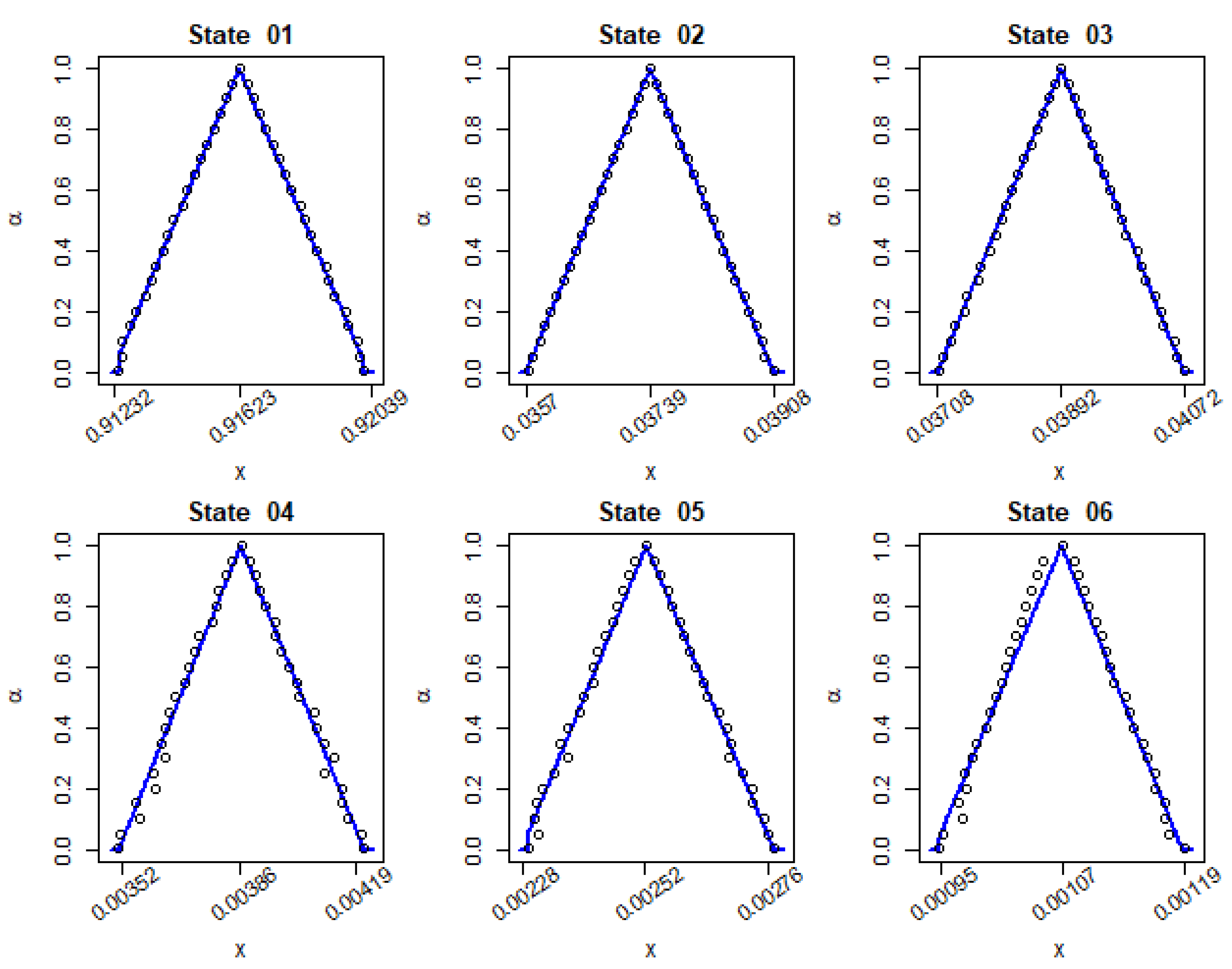
Once the fuzzy transition matrix associated with the FBMS has been obtained, to determine the fuzzy stationary state, Steps 1 to 4 in Section 3.2 should be applied and, therefore, optimization problems in Equations (23) and (24) must be solved. Notice that although the probabilities ${\tilde{\pi }}_j$, $j=1,\dots ,r$, are obtained by solving complex optimization problems, the results of the numerical applications 4 and 5, that have been obtained with the R package FuzzyStatProb by [13] (see Figure 1 and Figure 2) suggest that its triangular approximate by using Equation (18), ${\tilde{\pi }}_j^{\prime }=\left({\pi }_{jL}/{\pi }_{jC}/{\pi }_{jU}\right)=\left(\underset{\_}{{\pi }_j}\left(0\right)/\underset{\_}{{\pi }_j}\left(1\right)=\overline{{\pi }_j}\left(1\right)/\overline{{\pi }_j}\left(0\right)\right)$ provides a satisfactory fitting.

Numerical Application 4. Now we compute the fuzzy stationary distribution $\left({\tilde{\pi }}_1,{\tilde{\pi }}_2,{\tilde{\pi }}_3\right)$ for the fuzzy transition matrix in numerical application 2. In order to do so, we use the R package FuzzyStatProb described in [13], which is based on the use of Equations (23) and (24). The pseudo-codes and codes used are included in Appendix A and Appendix B, respectively, and the result of $\left({\tilde{\pi }}_1,{\tilde{\pi }}_2,{\tilde{\pi }}_3\right)$ in Figure 2.

It should be remarked that the probabilities obtained by [11] (p. 847) are intervals whose values are the $0$-cuts of the probabilities in our FMC.

Numerical Application 5. Let us consider the Irish BMS in numerical application 3.

Table 4. Results of the Irish BMS when $\tilde{\lambda }=\left(0.038/0.04/0.042\right)$—supports and cores.

Stationary Probabilities	$\mathit{\alpha }=\mathbf{0}$	$\mathit{\alpha }=\mathbf{1}$
${\tilde{\pi }}_1$	$\lceil 0.912318,0.920394\rceil$	0.916232
${\tilde{\pi }}_2$	$\lceil 0.035705,0.039075\rceil$	0.037394
${\tilde{\pi }}_3$	$\lceil 0.037080,0.040717\rceil$	0.038921
${\tilde{\pi }}_4$	$\lceil 0.003519,0.004186\rceil$	0.003861
${\tilde{\pi }}_5$	$\lceil 0.002275,0.002758\rceil$	0.002523
${\tilde{\pi }}_6$	$\lceil 0.000954,0.001190\rceil$	0.001069

Source: Own elaboration.

shows the supports and cores of the fuzzy stationary state ${\tilde{\pi }}_j$, $j=1,\dots ,6$ when considering fuzzy probabilities in Equations (37)–(40). The pseudo-codes and the codes of the R package FuzzyStatProb that have been used to get these results are included in Appendix A and Appendix B, respectively. Figure 3 depicts the graphical representation of ${\tilde{\pi }}_j$, $j=1,\dots ,6$.

The shape of the fuzzy stationary distribution suggests that their triangular approximate must work quite well.

Table 5. $\alpha$-cuts of ${\tilde{\pi }}_4$, it’s triangular approximate, ${\tilde{\pi }}_4^{\prime }$, and errors.

	${\mathit{\pi }}_{\mathbf{4}}\mathbf{\left(}\mathit{\alpha }\mathbf{\right)}$		${\mathit{\pi }}_{\mathbf{4}}^{\mathbf{\prime }}\mathbf{\left(}\mathit{\alpha }\mathbf{\right)}$		Error *
$\mathit{\alpha }$	$\underset{\_}{{\mathit{\pi }}_{\mathbf{4}}}\mathbf{\left(}\mathit{\alpha }\mathbf{\right)}$	$\overline{{\mathit{\pi }}_{\mathbf{4}}}\mathbf{\left(}\mathit{\alpha }\mathbf{\right)}$	$\underset{\_}{{\mathit{\pi }}_{\mathbf{4}}^{\mathbf{\prime }}}\mathbf{\left(}\mathit{\alpha }\mathbf{\right)}$	$\overline{{\mathit{\pi }}_{\mathbf{4}}^{\mathbf{\prime }}}\mathbf{\left(}\mathit{\alpha }\mathbf{\right)}$	$\underset{\_}{\mathit{e}\mathit{r}\mathit{r}}\mathbf{\left(}\mathit{\alpha }\mathbf{\right)}$	$\overline{\mathit{e}\mathit{r}\mathit{r}}\mathbf{\left(}\mathit{\alpha }\mathbf{\right)}$
1	0.00386	0.00386	0.00386	0.00386	0.000%	0.000%
0.9	0.00381	0.00390	0.00383	0.00389	0.345%	0.188%
0.8	0.00379	0.00393	0.00379	0.00393	0.092%	0.082%
0.7	0.00375	0.00398	0.00376	0.00396	0.368%	0.405%
0.6	0.00371	0.00400	0.00372	0.00399	0.442%	0.145%
0.5	0.00368	0.00403	0.00369	0.00402	0.289%	0.194%
0.4	0.00364	0.00408	0.00366	0.00406	0.324%	0.474%
0.3	0.00360	0.00411	0.00362	0.00409	0.537%	0.484%
0.2	0.00356	0.00413	0.00359	0.00412	0.655%	0.272%
0.1	0.00354	0.00418	0.00355	0.00415	0.406%	0.550%
0	0.00352	0.00419	0.00352	0.00419	0.000%	0.000%

Source: Own elaboration. * $\underset{\_}{err}\left(\alpha \right)=\frac{\left|\underset{\_}{{\pi }_4}\left(\alpha \right)-\underset{\_}{{\pi }_4^{\prime }}\left(\alpha \right)\right|}{\underset{\_}{{\pi }_4}\left(\alpha \right)}$ and $\overline{err}\left(\alpha \right)=\frac{\left|\overline{{\pi }_4}\left(\alpha \right)-\overline{{\pi }_4^{\prime }}\left(\alpha \right)\right|}{\overline{{\pi }_4}\left(\alpha \right)}$.

shows that the relative deviations of the lower and upper bounds of the approximate of ${\tilde{\pi }}_4$, ${\pi }_4^{\prime }\left(\alpha \right),$ with respect to the respective bounds of ${\pi }_4\left(\alpha \right)$ are always under 1%. Therefore, the above intuition is confirmed in the case of ${\tilde{\pi }}_4$. We have also observed that this fact also applies to the other stationary probabilities in the numerical application. So, it can be written:

$${\tilde{\pi }}_1\approx \left(0.912318/0.916232/0.920394\right).$$

$${\tilde{\pi }}_2\approx \left(0.035705/0.037394/0.039075\right).$$

$${\tilde{\pi }}_3\approx \left(0.037080/0.038921/0.040717\right).$$

$${\tilde{\pi }}_4\approx \left(0.003519/0.003861/0.004186\right).$$

$${\tilde{\pi }}_5\approx \left(0.002275/0.002523/0.002758\right).$$

$${\tilde{\pi }}_6\approx \left(0.000954/0.001069/0.001190\right).$$

It is worth pointing out that the intervals fitted for the stationary state in [11] (p. 848) are the 0-cuts of ${\tilde{\pi }}_j$, $j=1,\dots ,6$, in the fuzzy version of the Irish BMS.

Two considerations are worth highlighting:

• FBMSs generalize the results of crisp and modal interval BMSs as can be checked by comparing the results of numerical applications 1 and 5. The results of the crisp case are exactly the 1-cut of estimates from FBMSs whereas the estimates obtained by [11] (p. 848) coincide, except in the order of the interval lower and upper bounds in some cases, with the 0-cut of the results by our FBMSs. Likewise, operating by means of $\alpha$-cuts allows obtaining the simulations of intermediate scenarios between that of maximum fuzziness (generated by the 0-cut of $\tilde{\lambda }$) and that with maximum reliability (that comes from $\lambda \left(1\right)$), as well as their grade of possibility. This information can be extremely useful to the decision-maker since it makes easier the sensitivity analysis for each possible value of Poisson parameter $\lambda$.
• Although a TFN $\tilde{\lambda }$ does not produce triangular probabilities ${\tilde{p}}_{ij}^{\left(n\right)}$ and ${\tilde{\pi }}_j$, their triangular approximates work pretty well. We consider this result interesting for two reasons:

  (a)

  The calculations can be done easily with less computational effort. For example, in the two first rows of Table 5, we have performed the calculations on a scale with eleven grades of possibility. So, 20 optimization programs have been solved for a single probability (10 minimizing programs for the lower bounds of $\alpha$-cuts $\alpha =0,0.1,\dots ,0.9$, and other 10 maximizing programs for the respective upper bounds). Likewise, obtaining the 1-cut implies nothing but solving a conventional Markov chain. This computational effort is reduced drastically by using the triangular approximate in Equation (18), which leads us to obtain the results in columns 3 and 4 of Table 5. In this case, it is enough to solve 2 optimization programs (1 minimizing program for the lower bound of the 0-cut and 1 maximizing for the upper one) and also, of course, evaluating a conventional BMS in ${\lambda }_C$. The interest in this result is amplified by the fact that the Irish BMS is relatively simple (there are 6 classes) and so it embeds only 36 ${\tilde{p}}_{ij}^{\left(n\right)}$ and 6 probabilities ${\tilde{\pi }}_j$. However, BMSs often have more than 20 classes (e.g., Belgian or German BMSs).

  (b)

  From the perspective of an actuary, a triangular approximate of the fuzzy probabilities can be very useful. A TFN provides an estimate of the most feasible, minimum, and maximum probability that can be interpreted intuitively without any knowledge of fuzzy set theory (FST). Therefore, the triangular approximates presented in this paper could facilitate the use of FBMSs in the insurance industry.

Step 4. Obtain the mean asymptotic premium, $b^{*}$.

In order to obtain the asymptotic mean premium, we have to evaluate the fuzzy version of Equation (4), ${\tilde{b}}^{*}={\displaystyle \sum }_{j=1}^r{b}_j{\tilde{\pi }}_j$. Bearing in mind Equations (12)–(14), (16) and (17), we first consider the domain:

$$Dom\left(\alpha \right)=\left\{{\pi }_j\in \left[\underset{\_}{{\pi }_j}\left(\alpha \right),\overline{{\pi }_j}\left(\alpha \right)\right],{\displaystyle \sum }_{j=1}^r{\pi }_j=1\right\}$$

(45)

and then the set $\left\{b^{*}={\displaystyle \sum }_{j=1}^r{b}_j{\pi }_j|{\pi }_j\in Dom\left(\alpha \right)\right\}$. The $\alpha$-cuts of ${\tilde{b}}^{*}$, $b^{*}\left(\alpha \right)=\left[\underset{\_}{b^{*}}\left(\alpha \right),\overline{b^{*}}\left(\alpha \right)\right]$, are obtained by solving:

$$\underset{\_}{b^{*}}\left(\alpha \right)=\min \left\{b^{*}={\displaystyle \sum }_{j=1}^r{b}_j{\pi }_j|{\pi }_j\in \left[\underset{\_}{{\pi }_j}\left(\alpha \right),\overline{{\pi }_j}\left(\alpha \right)\right],{\displaystyle \sum }_{j=1}^r{\pi }_j=1\right\}$$

(46)

$$\overline{b^{*}}\left(\alpha \right)=\max \left\{b^{*}={\displaystyle \sum }_{j=1}^r{b}_j{\pi }_j|{\pi }_j\in \left[\underset{\_}{{\pi }_j}\left(\alpha \right),\overline{{\pi }_j}\left(\alpha \right)\right],{\displaystyle \sum }_{j=1}^r{\pi }_j=1\right\}$$

(47)

which are linear programming problems and so solvable, e.g., with the simplex algorithm. In fact, the problem to solve in this case is the same as that in [35].

A triangular approximate for ${\tilde{b}}^{*},{\tilde{b}}^{*{}^{\prime }}=\left(b_L^{*}/b_C^{*}/b_U^{*}\right)$, can be obtained by using the 0-cut and the 1-cut obtained from Equations (46) and (47) or, alternatively, if these results have not been previously calculated, by considering the TFNs $\left({\pi }_j{}_L/{\pi }_{jC}/{\pi }_j{}_U\right),j=1,\dots ,r$, and solving the following linear problems:

$$b_L^{*}=\min \left\{b^{*}={\displaystyle \sum }_{j=1}^r{b}_j{\pi }_j|{\pi }_j\in \left[{\pi }_j{}_L,{\pi }_j{}_U\right],{\displaystyle \sum }_{j=1}^r{\pi }_j=1\right\}$$

(48)

$$b_U^{*}=\max \left\{b^{*}={\displaystyle \sum }_{j=1}^r{b}_j{\pi }_j|{\pi }_j\in \left[{\pi }_j{}_L,{\pi }_j{}_U\right],{\displaystyle \sum }_{j=1}^r{\pi }_j=1\right\}$$

(49)

In this latter way, 20 linear problems that come from Expressions (46) and (47) when ${\tilde{b}}^{*}$ is performed with a scale of eleven grades of possibility are reduced to 2 linear programs. Moreover:

$$b_C^{*}={\displaystyle \sum }_{j=1}^r{b}_j{\pi }_{jC}$$

(50)

Numerical Application 6. Let us consider again the Irish BMS in numerical application 3, i.e., $N~\mathrm{Po}\left(\left(0.038/0.04/0.042\right)\right)$. By using the premium level of each class (see Table 2), we obtain the $\alpha$-cuts of the fuzzy mean asymptotic premium, ${\tilde{b}}^{*}$, from Equations (45)–(47). These results are in

Table 6. $\alpha$-cuts of ${\tilde{b}}^{*},$ it’s triangular approximate ${\tilde{b}}^{*{}^{\prime }}$ and its errors.

	${\mathit{b}}^{\mathbf{*}}\mathbf{\left(}\mathit{\alpha }\mathbf{\right)}$		${\mathit{b}}^{\mathbf{*}{}^{\mathbf{\prime }}}\mathbf{\left(}\mathit{\alpha }\mathbf{\right)}$		Error *
$\mathit{\alpha }$	$\underset{\_}{{\mathit{b}}^{\mathbf{*}}}\mathbf{\left(}\mathit{\alpha }\mathbf{\right)}$	$\overline{{\mathit{b}}^{\mathbf{*}}}\mathbf{\left(}\mathit{\alpha }\mathbf{\right)}$	${\underset{\_}{{\mathit{b}}^{\mathbf{*}}}}^{\mathbf{\prime }}\mathbf{\left(}\mathit{\alpha }\mathbf{\right)}$	$\overline{{\mathit{b}}^{\mathbf{*}{}^{\mathbf{\prime }}}}\mathbf{\left(}\mathit{\alpha }\mathbf{\right)}$	$\underset{\_}{\mathit{e}\mathit{r}\mathit{r}}\mathbf{\left(}\mathit{\alpha }\mathbf{\right)}$	$\overline{\mathit{e}\mathit{r}\mathit{r}}\mathbf{\left(}\mathit{\alpha }\mathbf{\right)}$
1	51.423	51.423	51.423	51.423	0.000%	0.000%
0.9	51.415	51.430	51.415	51.430	0.000%	0.000%
0.8	51.407	51.438	51.407	51.438	0.000%	0.000%
0.7	51.399	51.445	51.399	51.445	0.000%	0.000%
0.6	51.391	51.453	51.391	51.453	0.000%	0.000%
0.5	51.383	51.460	51.383	51.460	0.000%	0.000%
0.4	51.375	51.468	51.375	51.468	0.000%	0.000%
0.3	51.367	51.475	51.367	51.475	0.000%	0.000%
0.2	51.359	51.483	51.359	51.483	0.000%	0.000%
0.1	51.352	51.491	51.352	51.491	0.000%	0.000%
0	51.344	51.498	51.344	51.498	0.000%	0.000%

Source: Own elaboration. * $\underset{\_}{err}\left(\alpha \right)=\frac{\left|\underset{\_}{b^{*}}\left(\alpha \right)-\underset{\_}{b^{*{}^{\prime }}}\left(\alpha \right)\right|}{\underset{\_}{b^{*}}\left(\alpha \right)}$ and $\overline{err}\left(\alpha \right)=\frac{\left|\overline{b^{*}}\left(\alpha \right)-\overline{b^{*{}^{\prime }}}\left(\alpha \right)\right|}{\overline{b^{*}}\left(\alpha \right)}$.

, which also show the $\alpha$-cuts of its triangular approximate, ${\tilde{b}}^{*{}^{\prime }}$, by Equations (48)–(50). From that table, it can be seen that ${\tilde{b}}^{*}$ is practically triangular since the errors by $b^{\prime }\left(\alpha \right)$ in fitting $b\left(\alpha \right)$ are negligible. Notice that the triangular approximate ${\tilde{b}}^{*{}^{\prime }}$ provides a straightforward generalization of both the point estimate by a crisp BMS, 51.423, as well as the modal interval estimate in [11] (p. 849), [51.344, 51.498].

5. Sensitivity Analysis

In this Section, we evaluate the sensitivity of the errors of the triangular approximates seen in Section 4 with respect to the parameter $\lambda$. The following assumptions are considered:

• The core of $\tilde{\lambda }$ may be low (0.04), medium (0.5), or high (0.96).
• The uncertainty of $\tilde{\lambda }$, which can be measured by its spreads, is symmetrical, i.e., left and right spreads are equal. This uncertainty can take two possible values: 0.002 or 0.015.
• We use the Irish BMS in Table 2.

Only results for $\tilde{p}\left(N\ge 1\right)$ and ${\tilde{\pi }}_4$ are shown. Furthermore, in order to avoid very long calculations, we have performed them on a scale with five grades of possibility. However, it can be verified that for other transition and stationary probabilities, and for a greater scale of grades of possibility, the conclusions to be drawn are practically the same.

Table 7. $\alpha$-cuts of $\tilde{p}\left(N\ge 1\right)$ and ${\tilde{\pi }}_4$, their triangular approximate and errors for different parameters $\tilde{\lambda }$.

	$\tilde{\mathit{\lambda }}=\left(\mathbf{0.038}/\mathbf{0.04}/\mathbf{0.042}\right)$
	${\tilde{\mathit{p}}}^{\prime }\left(\mathit{N}\ge \mathbf{1}\right)=\left(\mathbf{0.03729}/\mathbf{0.03921}/\mathbf{0.04113}\right)$				${\tilde{\mathit{\pi }}}_{\mathbf{4}}^{\prime }=\left(\mathbf{0.00352}/\mathbf{0.00386}/\mathbf{0.00419}\right)$
	$\mathit{p}\left(\mathit{N}\ge \mathbf{1}\right)\left(\mathit{\alpha }\right)$		Error		${\mathit{\pi }}_{\mathbf{4}}\left(\mathit{\alpha }\right)$		Error
$\alpha$	$\underset{\_}{p\left(N\ge 1\right)}\left(\alpha \right)$	$\overline{p\left(N\ge 1\right)}\left(\alpha \right)$	$\underset{\_}{err}\left(\alpha \right)$	$\overline{err}\left(\alpha \right)$	$\underset{\_}{{\pi }_4}\left(\alpha \right)$	$\overline{{\pi }_4}\left(\alpha \right)$	$\underset{\_}{err}\left(\alpha \right)$	$\overline{err}\left(\alpha \right)$
1	0.03921	0.03921	0.000%	0.000%	0.00386	0.00386	0.000%	0.000%
0.75	0.03873	0.03969	0.001%	0.001%	0.00376	0.00395	0.044%	0.041%
0.5	0.03825	0.04017	0.001%	0.001%	0.00367	0.00405	0.060%	0.054%
0.25	0.03777	0.04065	0.001%	0.001%	0.00358	0.00415	0.046%	0.039%
0	0.03729	0.04113	0.000%	0.000%	0.00352	0.00419	0.000%	0.000%
	$\tilde{\mathit{\lambda }}=\left(\mathbf{0.025}/\mathbf{0.04}/\mathbf{0.055}\right)$
	${\tilde{\mathit{p}}}^{\prime }\left(\mathit{N}\ge \mathbf{1}\right)=\left(\mathbf{0.02469}/\mathbf{0.03921}/\mathbf{0.05351}\right)$				${\tilde{\mathit{\pi }}}_{\mathbf{4}}^{\prime }=\left(\mathbf{0.00153}/\mathbf{0.00386}/\mathbf{0.00717}\right)$
	$\mathit{p}\left(\mathit{N}\ge \mathbf{1}\right)\left(\mathit{\alpha }\right)$		Error		${\mathit{\pi }}_{\mathbf{4}}\left(\mathit{\alpha }\right)$		Error
$\alpha$	$\underset{\_}{p\left(N\ge 1\right)}\left(\alpha \right)$	$\overline{p\left(N\ge 1\right)}\left(\alpha \right)$	$\underset{\_}{err}\left(\alpha \right)$	$\overline{err}\left(\alpha \right)$	$\underset{\_}{{\pi }_4}\left(\alpha \right)$	$\overline{{\pi }_4}\left(\alpha \right)$	$\underset{\_}{err}\left(\alpha \right)$	$\overline{err}\left(\alpha \right)$
1	0.03921	0.03921	0.000%	0.000%	0.00386	0.00386	0.000%	0.000%
0.75	0.03560	0.04281	0.057%	0.047%	0.00318	0.00460	2.985%	1.955%
0.5	0.03198	0.04639	0.085%	0.058%	0.00257	0.00540	4.958%	2.208%
0.25	0.02834	0.04996	0.072%	0.040%	0.00202	0.00626	4.757%	1.420%
0	0.02469	0.05351	0.000%	0.000%	0.00153	0.00717	0.000%	0.000%
	$\tilde{\mathit{\lambda }}=\left(\mathbf{0.498}/\mathbf{0.05}/\mathbf{0.502}\right)$
	${\tilde{\mathit{p}}}^{\prime }\left(\mathit{N}\ge \mathbf{1}\right)=\left(\mathbf{0.39226}/\mathbf{0.39347}/\mathbf{0.39468}\right)$				${\tilde{\mathit{\pi }}}_{\mathbf{4}}^{\prime }=\left(\mathbf{0.15617}/\mathbf{0.15618}/\mathbf{0.15618}\right)$
	$\mathit{p}\left(N\ge \mathbf{1}\right)\left(\mathit{\alpha }\right)$		Error		${\mathit{\pi }}_{\mathbf{4}}\left(\alpha \right)$		Error
$\alpha$	$\underset{\_}{p\left(N\ge 1\right)}\left(\alpha \right)$	$\overline{p\left(N\ge 1\right)}\left(\alpha \right)$	$\underset{\_}{err}\left(\alpha \right)$	$\overline{err}\left(\alpha \right)$	$\underset{\_}{{\pi }_4}\left(\alpha \right)$	$\overline{{\pi }_4}\left(\alpha \right)$	$\underset{\_}{err}\left(\alpha \right)$	$\overline{err}\left(\alpha \right)$
1	0.39347	0.39347	0.000%	0.000%	0.15618	0.15618	0.000%	0.000%
0.75	0.39317	0.39377	0.000%	0.000%	0.15617	0.15618	0.000%	0.000%
0.5	0.39286	0.39408	0.000%	0.000%	0.15617	0.15618	0.001%	0.001%
0.25	0.39256	0.39438	0.000%	0.000%	0.15617	0.15618	0.000%	0.000%
0	0.39226	0.39468	0.000%	0.000%	0.15617	0.15618	0.000%	0.000%
	$\tilde{\mathit{\lambda }}=\left(\mathbf{0.485}/\mathbf{0.5}/\mathbf{0.515}\right)$
	${\tilde{\mathit{p}}}^{\prime }\left(\mathit{N}\ge \mathbf{1}\right)=(\mathbf{0.38430}/\mathbf{0.39347}/\mathbf{0.40250}$)				${\tilde{\mathit{\pi }}}_{\mathbf{4}}^{\prime }=\left(\mathbf{0.15596}/\mathbf{0.15618}/\mathbf{0.15625}\right)$
	$\mathit{p}\left(\mathit{N}\ge \mathbf{1}\right)\left(\mathit{\alpha }\right)$		Error		${\mathit{\pi }}_{\mathbf{4}}\left(\alpha \right)$		Error
$\alpha$	$\underset{\_}{p\left(N\ge 1\right)}\left(\alpha \right)$	$\overline{p\left(N\ge 1\right)}\left(\alpha \right)$	$\underset{\_}{err}\left(\alpha \right)$	$\overline{err}\left(\alpha \right)$	$\underset{\_}{{\pi }_4}\left(\alpha \right)$	$\overline{{\pi }_4}\left(\alpha \right)$	$\underset{\_}{err}\left(\alpha \right)$	$\overline{err}\left(\alpha \right)$
1	0.39347	0.39347	0.000%	0.000%	0.15618	0.15618	0.000%	0.000%
0.75	0.39119	0.39574	0.003%	0.003%	0.15615	0.15618	0.024%	0.023%
0.5	0.38890	0.39800	0.004%	0.004%	0.15611	0.15620	0.032%	0.030%
0.25	0.38661	0.40025	0.003%	0.003%	0.15604	0.15623	0.024%	0.022%
0	0.38430	0.40250	0.000%	0.000%	0.15596	0.15625	0.000%	0.000%
	$\tilde{\mathit{\lambda }}=\left(\mathbf{0.958}/\mathbf{0.96}/\mathbf{0.962}\right)$
	${\tilde{\mathit{p}}}^{\prime }\left(\mathit{N}\ge \mathbf{1}\right)=\left(\mathbf{0.61634}/\mathbf{0.61711}/\mathbf{0.61787}\right)$				${\tilde{\mathit{\pi }}}_{\mathbf{4}}^{\prime }=\left(\mathbf{0.09820}/\mathbf{0.09850}/\mathbf{0.09879}\right)$
	$\mathit{p}\left(\mathit{N}\ge \mathbf{1}\right)\left(\mathit{\alpha }\right)$		Error		${\mathit{\pi }}_{\mathbf{4}}\left(\mathit{\alpha }\right)$		Error
$\alpha$	$\underset{\_}{p\left(N\ge 1\right)}\left(\alpha \right)$	$\overline{p\left(N\ge 1\right)}\left(\alpha \right)$	$\underset{\_}{err}\left(\alpha \right)$	$\overline{err}\left(\alpha \right)$	$\underset{\_}{{\pi }_4}\left(\alpha \right)$	$\overline{{\pi }_4}\left(\alpha \right)$	$\underset{\_}{err}\left(\alpha \right)$	$\overline{err}\left(\alpha \right)$
1	0.61711	0.61711	0.000%	0.000%	0.09850	0.09850	0.000%	0.000%
0.75	0.61692	0.61730	0.000%	0.000%	0.09842	0.09857	0.000%	0.000%
0.5	0.61672	0.61749	0.000%	0.000%	0.09835	0.09864	0.000%	0.000%
0.25	0.61653	0.61768	0.000%	0.000%	0.09827	0.09872	0.000%	0.000%
0	0.61634	0.61787	0.000%	0.000%	0.09820	0.09879	0.000%	0.000%
	$\tilde{\mathit{\lambda }}=\left(\mathbf{0.0945}/\mathbf{0.96}/\mathbf{0.0975}\right)$
	${\tilde{\mathit{p}}}^{\prime }\left(\mathit{N}\ge \mathbf{1}\right)=\left(\mathbf{0.61132}/\mathbf{0.61711}/\mathbf{0.62281}\right)$				${\tilde{\mathit{\pi }}}_{\mathbf{4}}^{\prime }=\left(\mathbf{0.09628}/\mathbf{0.09850}/\mathbf{0.10074}\right)$
	$\mathit{p}\left(\mathit{N}\ge \mathbf{1}\right)\left(\mathit{\alpha }\right)$		Error		${\mathit{\pi }}_{\mathbf{4}}\left(\mathit{\alpha }\right)$		Error
$\alpha$	$\underset{\_}{p\left(N\ge 1\right)}\left(\alpha \right)$	$\overline{p\left(N\ge 1\right)}\left(\alpha \right)$	$\underset{\_}{err}\left(\alpha \right)$	$\overline{err}\left(\alpha \right)$	$\underset{\_}{{\pi }_4}\left(\alpha \right)$	$\overline{{\pi }_4}\left(\alpha \right)$	$\underset{\_}{err}\left(\alpha \right)$	$\overline{err}\left(\alpha \right)$
1	0.61711	0.61711	0.000%	0.000%	0.09850	0.09850	0.000%	0.000%
0.75	0.61567	0.61854	0.001%	0.001%	0.09794	0.09905	0.003%	0.003%
0.5	0.61422	0.61997	0.002%	0.002%	0.09738	0.09962	0.004%	0.003%
0.25	0.61278	0.62139	0.001%	0.001%	0.09683	0.10018	0.003%	0.003%
0	0.61132	0.62281	0.000%	0.000%	0.09628	0.10074	0.000%	0.000%

Source: Own Elaboration.

shows that:

• The goodness of triangular approximates is always better than acceptable as can be checked in Table 7. In the worst case, for ${\tilde{\pi }}_4$, $\alpha =0.5$ and risk parameter $\tilde{\lambda }=0.025/0.04/0.055$, errors are below 5%.
• Errors (as defined for Table 3 and Table 5) increase with respect to the uncertainty of risk parameter and decrease with respect to the value of its core.

Table 8. $\alpha$-cuts of ${\tilde{b}}^{*}$, it’s triangular approximate and errors for different parameters $\tilde{\lambda }$.

	$\tilde{\mathit{\lambda }}\mathbf{=}\mathbf{\left(}\mathbf{0.025}\mathbf{/}\mathbf{0.04}\mathbf{/}\mathbf{0.055}\mathbf{\right)}$				$\tilde{\mathit{\lambda }}\mathbf{=}\mathbf{\left(}\mathbf{0.485}\mathbf{/}\mathbf{0.5}\mathbf{/}\mathbf{0.515}\mathbf{\right)}$				$\tilde{\mathit{\lambda }}\mathbf{=}\mathbf{\left(}\mathbf{0.0945}\mathbf{/}\mathbf{0.96}\mathbf{/}\mathbf{0.0975}\mathbf{\right)}$
	${\tilde{\mathit{b}}}^{\mathbf{*}{}^{\mathbf{\prime }}}\mathbf{=}\mathbf{\left(}\mathbf{50.836}\mathbf{/}\mathbf{51.422}\mathbf{/}\mathbf{52.073}\mathbf{\right)}$				${\tilde{\mathit{b}}}^{\mathbf{*}{}^{\mathbf{\prime }}}\mathbf{=}\mathbf{\left(}\mathbf{80.662}\mathbf{/}\mathbf{81.396}\mathbf{/}\mathbf{82.098}\mathbf{\right)}$				${\tilde{\mathit{b}}}^{\mathbf{*}{}^{\mathbf{\prime }}}\mathbf{=}\mathbf{\left(}\mathbf{93.058}\mathbf{/}\mathbf{93.246}\mathbf{/}\mathbf{93.427}\mathbf{\right)}$
	${\mathit{b}}^{\mathbf{*}}\mathbf{\left(}\mathit{\alpha }\mathbf{\right)}$		Error		${\mathit{b}}^{\mathbf{*}}\mathbf{\left(}\mathit{\alpha }\mathbf{\right)}$		Error		${\mathit{b}}^{\mathbf{*}}\mathbf{\left(}\mathit{\alpha }\mathbf{\right)}$		Error
$\alpha$	$\underset{\_}{b^{\mathbf{*}}}\mathbf{\left(}\alpha \mathbf{\right)}$	$\overline{b^{\mathbf{*}}}\mathbf{\left(}\alpha \mathbf{\right)}$	$\underset{\_}{err}\mathbf{\left(}\alpha \mathbf{\right)}$	$\overline{err}\mathbf{\left(}\alpha \mathbf{\right)}$	$\underset{\_}{b^{\mathbf{*}}}\mathbf{\left(}\alpha \mathbf{\right)}$	$\overline{b^{\mathbf{*}}}\mathbf{\left(}\alpha \mathbf{\right)}$	$\underset{\_}{err}\mathbf{\left(}\alpha \mathbf{\right)}$	$\overline{err}\mathbf{\left(}\alpha \mathbf{\right)}$	$\underset{\_}{b^{\mathbf{*}}}\mathbf{\left(}\alpha \mathbf{\right)}$	$\overline{b^{\mathbf{*}}}\mathbf{\left(}\alpha \mathbf{\right)}$	$\underset{\_}{err}\mathbf{\left(}\alpha \mathbf{\right)}$	$\overline{err}\mathbf{\left(}\alpha \mathbf{\right)}$
1	51.422	51.422	0.000%	0.000%	81.396	81.396	0.000%	0.000%	93.246	93.246	0.000%	0.000%
0.75	51.270	51.579	0.012%	0.012%	81.215	81.574	0.004%	0.004%	93.200	93.292	0.001%	0.001%
0.5	51.121	51.739	0.016%	0.016%	81.033	81.751	0.005%	0.005%	93.153	93.338	0.001%	0.001%
0.25	50.977	51.904	0.012%	0.012%	80.848	81.925	0.004%	0.004%	93.106	93.383	0.001%	0.001%
0	50.836	52.073	0.000%	0.000%	80.662	82.098	0.000%	0.000%	93.058	93.427	0.000%	0.000%

Source: Own Elaboration.

shows the mean asymptotic premiums for the cores of $\tilde{\lambda }$ considered in Table 7 and the most uncertain scenario (left and right spread equal to 0.015). It can be checked that triangular approximates ${\tilde{b}}^{*{}^{\prime }}$ always reach a practically perfect match to ${\tilde{b}}^{*}$, i.e., errors (as defined for Table 6) are very close to 0.

6. Summary and Further Research

BMSs are often modelled by means of MCs with crisp probabilities. In this paper, it is considered that transition probabilities of Markovian BMSs are not crisp but uncertain. This uncertainty is captured by using a FN, thus giving rise to the concept of FBMSs. FBMSs modeling is based on the concept of FMC by Buckley and Eslami in [12]. As a result, conventional BMSs can be understood as a particular case of our model where transition probabilities are singletons. The model in [11] represents the uncertainty by means of modal intervals. Since its results can be interpreted as the 0-cuts of ours, that model can also be seen as a particular case of our FBMS.

We assume, as it is often done in actuarial literature, that the number of claims in a period is a Poisson RV. Nonetheless, due to uncertainty, its parameter $\lambda$ is not a real number but a TFN. So, to implement the model presented in the paper, it is necessary, firstly, to structure available information of the behavior of that RV. From this information, the Poisson parameter can be fitted by means of a TFN. Three alternatives to do so are proposed. Subsequently, by using $\alpha$-cut arithmetic, transition probabilities, the stationary distribution function, and the mean asymptotic premium of the FBMS are obtained by means of their $\alpha$-cuts. The lower and upper bounds of these $\alpha$-cuts can be understood as the result of a sensitivity analysis of the BMS that evaluates two extreme scenarios with possibility $\alpha$. That output can be very useful in actuarial decision-making processes since it provides a set of sensitivity analyses that is structured on the basis of their grade of reliability.

Although the mean number of claims, $\lambda$, is assumed to be a TFN, the outputs from our FBMS do not maintain that shape. However, in the numerical applications developed within the framework of the Irish BMS, we have verified that all the outputs obtained from a triangular $\lambda$ are well approximated by a TFN that maintains the support and core of the original FN. This result is quite interesting. On the one hand, other more complex shapes of FNs can produce drawbacks in information modeling, such as problems with calculations in computer implementation. In this regard, we have observed that the number of optimizing problems to be solved in order to obtain transition probabilities, the stationary distribution, and the mean asymptotic premium is reduced drastically. Likewise, TFNs are very attractive from an insurance decision-making perspective since TFNs admit a very intuitive interpretation even without any knowledge of FST. At least, a TFN provides an estimate of the maximum, minimum, and most feasible values of a variable. Therefore, we feel that the triangular approximations introduced in this document would make it easier to use FMCs in the implementation of BMSs by the insurance industry.

Our methodologic approach can be extended, with the necessary adaptations, to other assumptions for the RV number of claims. Likewise, as far as we are concerned, there are several topics that may be the object of further research. Firstly, a wider investigation on how to apply a fuzzy Poisson regression in a BMS context must be carried out. Secondly, a more in-depth evaluation of the goodness of triangular approximations to BMS probabilities and the mean asymptotic premium is needed. In this respect, a wider range for the values of $\lambda$, a greater number of classes in the BMS, and other methods to fit triangular approximates must be tested. Thirdly, it is also needed to extend our model to the case in which fuzzy uncertainty in the BMS does not only appear in the number of claims but also their cost. Moreover, to model $\lambda$, instead of TFNs, other types of FNs, such as GFNs or IFNs, could be considered. We are aware that these tools allow capturing uncertainty with more nuances than FNs. However, their fitting has a greater cost than TFNs since it implies adjusting more parameters. Additionally, implementing computational operations with them is more expensive. This last issue is crucial in our context, especially in complex BMSs like, e.g., the German one. So, we feel that applying FNs suppose a balance between the simplicity of crisp or interval probabilities and more complex representations of uncertain quantities such as GFNs or IFNs. Finally, to evaluate the efficiency of a BMS, it is usually calculated the elasticity of the mean premium (4) with respect to the risk parameter $\lambda$. To do so, numerical simulations for point values of $\lambda$ within the reference interval [0,1] are implemented (see, e.g., [2]). The use of fuzzy logic may be of interest in this concern. For example, that reference interval can be granulated into linguistic labels such as “low risk”, “medium risk” and so on, similarly to that proposed by [27] and [57]. Therefore, elasticity evaluations may be made on the basis of linguistic labels instead of point values on [0,1]. Fuzzy linguistic Markov chains, presented by [58], may be the starting point for this.

References

- Lemaire, J. Bonus-Malus Systems in Automobile Insurance; Kluwer Academic Publishers: Norwell, MA, USA, 1995. [Google Scholar]
- Lemaire, J.; Zi, H. A comparative analysis of 30 bonus-malus systems. ASTIN Bull. 1994, 24, 287–309. [Google Scholar] [CrossRef] [Green Version]
- Meyer, U. Third Party Motor Insurance in Europe. Comparative Study of the Economical-Statistical Situation. In Personal Communications; University of Bamberg: Bamberg, Germany, 2000. [Google Scholar]
- Dodu, D. Comparative Analysis of Bonus Malus Systems in Italy and Central and Eastern Europe. 2017. Available online: https://www.milliman.com/en/insight/comparative-analysis-of-bonus-malus-systems-in-italy-and-central-and-eastern-europe (accessed on 7 October 2020).
- Pitrebois, S.; Denuit, M.; Walhin, J.F. Fitting the Belgian bonus-malus system. Belg. Actuar. Bull. 2003, 3, 58–62. [Google Scholar]
- de Pril, N. The Efficiency of a Bonus-Malus System. ASTIN Bull. 1978, 10, 59–72. [Google Scholar] [CrossRef] [Green Version]
- Bonsdorff, H. On the convergence rate of bonus-malus systems. ASTIN Bull. 1992, 22, 217–223. [Google Scholar] [CrossRef] [Green Version]
- Pitrebois, S.; Denuit, M.; Walhin, J.F. Bonus-malus scales in segmented tariffs: Gilde & Sundt’s work revisited. Aust. Actuar. J. 2004, 10, 107–125. [Google Scholar]
- Niemiec, M. Bonus-Malus Systems as Markov Set-Chains. ASTIN Bull. 2007, 37, 53–65. [Google Scholar] [CrossRef] [Green Version]
- Asmussen, S. Modeling and performance of Bonus-Malus systems: Stationary versus age-correction. Risks 2014, 2, 49–73. [Google Scholar] [CrossRef] [Green Version]
- Adillon, R.; Lambert, J.; Mármol, M. Modal interval probability: Application to Bonus-Malus Systems. Int. J. Uncertain. Fuzziness Knowl. Based Syst. 2020, 28, 837–851. [Google Scholar] [CrossRef]
- Buckley, J.J.; Eslami, E. Fuzzy Markov Chains: Uncertain Probabilities. Mathw. Soft Comput. 2002, 9, 33–41. [Google Scholar]
- Villacorta, P.J.; Verdegay, J.L. FuzzyStatProb: An R Package for the Estimation of Fuzzy Stationary Probabilities from a Sequence of Observations of an Unknown Markov Chain. J. Stat. Softw. 2016, 71, 1–27. [Google Scholar] [CrossRef]
- Denuit, M.; Marchal, X.; Pitrebois, S.; Walhin, J.F. Actuarial Modelling of Claims Counts: Risk Classification, Credibility and Bonus-Malus Systems; Wiley: Chichester, UK, 2007. [Google Scholar]
- Vernic, R. On risk measures and capital allocation for distributions depending on parameters with interval or fuzzy uncertainty. Appl. Soft Comput. 2018, 64, 199–215. [Google Scholar] [CrossRef]
- Wierzchoń, S.T. Randomness and Fuzziness in A Linear Programming Problem. In Combining Fuzzy Imprecision with Probabilistic Uncertainty in Decision Making. Lecture Notes in Economics and Mathematical Systems; Kacprzyk, J., Fedrizzi, M., Eds.; Springer: Berlin, Germany, 1988; Volume 310, pp. 227–239. [Google Scholar] [CrossRef]
- Buckley, J.J. Uncertain probabilities III: The continuous case. Soft Comput. 2004, 8, 200–206. [Google Scholar] [CrossRef]
- Buckley, J.J.; Eslami, E. Uncertain probabilities II: The continuous case. Soft Comput. 2004, 8, 193–199. [Google Scholar] [CrossRef]
- Buckley, J.J.; Eslami, E. Uncertain probabilities I: The discrete case. Soft Comput. 2003, 7, 500–505. [Google Scholar] [CrossRef]
- Zmeškal, Z. Value at risk methodology under soft conditions approach (fuzzy-stochastic approach). Eur. J. Oper. Res. 2005, 161, 337–347. [Google Scholar] [CrossRef]
- Moussa, A.M.; Kamdem, J.S.; Terraza, M. Fuzzy value-at-risk and expected shortfall for portfolios with heavy-tailed returns. Econ. Model. 2014, 39, 247–256. [Google Scholar] [CrossRef]
- Shapiro, A.F. Fuzzy logic in insurance. Insur. Math. Econ. 2004, 35, 399–424. [Google Scholar] [CrossRef]
- Huang, T.; Zhao, R.; Tang, W. Risk model with fuzzy random individual claim amount. Eur. J. Oper. Res. 2009, 192, 879–890. [Google Scholar] [CrossRef]
- Kemaloglu, S.A.; Shapiro, A.F.; Tank, F.; Apaydin, A. Using fuzzy logic to interpret dependent risks. Insur. Math. Econ. 2018, 79, 101–106. [Google Scholar] [CrossRef]
- Koissi, M.C.; Shapiro, A.F. Fuzzy formulation of the Lee–Carter model for mortality forecasting. Insur. Math. Econ. 2006, 39, 287–309. [Google Scholar] [CrossRef]
- Shapiro, A.F. Modeling future lifetime as a fuzzy random variable. Insur. Math. Econ. 2013, 53, 864–870. [Google Scholar] [CrossRef]
- Andrés-Sánchez, J.D.; Puchades, L.G.V. Some computational results for the fuzzy random value of life actuarial liabilities. Iran. J. Fuzzy Syst. 2017, 14, 1–25. [Google Scholar] [CrossRef]
- Andrés-Sánchez, J.D.; Puchades, L.G.V. A Fuzzy-Random Extension of the Lee–Carter Mortality Prediction Model. Int. J. Comput. Intell. Syst. 2019, 12, 775–794. [Google Scholar] [CrossRef] [Green Version]
- Jorba, L.; Adillon, R. A Generalization of Trapezoidal Fuzzy Numbers Based on Modal Interval Theory. Symmetry 2017, 9, 198. [Google Scholar] [CrossRef] [Green Version]
- Loimaranta, K. Some Asymptotic Properties of Bonus Systems. ASTIN Bull. 1972, 6, 233–245. [Google Scholar] [CrossRef] [Green Version]
- Heras, A.; Vilar, J.L.; Gil, J.A. Asymptotic Fairness of Bonus-Malus Systems and Optimal Scales of Premiums. Geneva Pap. Risk Insur. Theory 2002, 27, 61–82. [Google Scholar] [CrossRef]
- Kafková, S. Bonus-malus systems in vehicle insurance. Procedia Econ. Financ. 2015, 23, 216–222. [Google Scholar] [CrossRef] [Green Version]
- Dong, W.; Shah, H.C. Vertex method for computing functions of fuzzy variables. Fuzzy Sets Syst. 1987, 24, 65–78. [Google Scholar] [CrossRef]
- Buckley, J.J.; Qu, Y. On using α-cuts to evaluate fuzzy equations. Fuzzy Sets Syst. 1990, 38, 309–312. [Google Scholar] [CrossRef]
- Dong, W.; Wong, F.S. Interactive fuzzy variables and fuzzy decisions. Fuzzy Sets Syst. 1989, 29, 1–19. [Google Scholar] [CrossRef]
- Kaufmann, A. Fuzzy Subsets Applications in O.R. and Management. In Fuzzy Set Theory and Applications; Jones, A., Kaufmann, A., Zimmermann, H.-J., Eds.; Springer: Dordrecht, The Netherlands, 1986; pp. 257–300. [Google Scholar] [CrossRef]
- Heberle, J.; Thomas, A. Combining chain-ladder reserving with fuzzy numbers. Insur. Math. Econ. 2014, 55, 96–104. [Google Scholar] [CrossRef]
- Jiménez, M.; Rivas, J.A. Fuzzy number approximation. Int. J. Uncertain. Fuzziness Knowl. Based Syst. 1998, 6, 69–78. [Google Scholar] [CrossRef]
- Grzegorzewski, P.; Pasternak-Winiarska, K. Natural trapezoidal approximations of fuzzy numbers. Fuzzy Sets Syst. 2014, 250, 90–109. [Google Scholar] [CrossRef]
- Grzegorzewski, P.; Mrówka, E. Trapezoidal approximations of fuzzy numbers. Fuzzy Sets Syst. 2005, 153, 115–135. [Google Scholar] [CrossRef]
- Kleyle, R.M.; de Korvin, A. Constructing one-step and limiting fuzzy transition probabilities for finite Markov chains. J. Intell. Fuzzy Syst. 1998, 6, 223–235. [Google Scholar]
- Zadeh, L.A. Fuzzy sets. Inf. Control. 1965, 8, 338–353. [Google Scholar] [CrossRef] [Green Version]
- Avrachenkov, K.E.; Sánchez, E. Fuzzy Markov Chains: Specificities and Properties. In Proceedings of the 8th IPMU’2000 Conference, Madrid, Spain, 3–7 July 2000; pp. 1851–1856. [Google Scholar]
- Li, G.; Xiu, B. Fuzzy Markov Chains Based on the Fuzzy Transition Probability. In Proceedings of the 26th Chinese Control and Decision Conference, Changsha, China, 31 May–2 June 2014; pp. 4351–4356. [Google Scholar] [CrossRef]
- Buckley, J.J. Fuzzy Probabilities: New Approach and Applications, Volume 115 of Studies in Fuzziness and Soft Computing, 2nd ed.; Springer: Heidelberg, Germany, 2005. [Google Scholar]
- Bardossy, A.; Duckstein, L.; Bogardi, I. Combination of fuzzy numbers representing expert opinions. Fuzzy Sets Syst. 1993, 57, 173–181. [Google Scholar] [CrossRef]
- Hsu, H.M.; Chen, C.T. Aggregation of fuzzy opinions under group decision making. Fuzzy Sets Syst. 1996, 79, 279–285. [Google Scholar] [CrossRef]
- Tsabadze, T. A method for aggregation of trapezoidal fuzzy estimates under group decision-making. Fuzzy Sets Syst. 2015, 266, 114–130. [Google Scholar] [CrossRef]
- Buckley, J.J. Fuzzy statistics: Regression and prediction. Soft Comput. 2005, 9, 769–775. [Google Scholar] [CrossRef]
- Sfiris, D.S.; Papadopoulos, B.K. Non-asymptotic fuzzy estimators based on confidence intervals. Inf. Sci. 2014, 279, 446–459. [Google Scholar] [CrossRef]
- Al-Kandari, M.; Adjenughwure, K.; Papadopoulos, K. A Fuzzy-Statistical Tolerance Interval from Residuals of Crisp Linear Regression Models. Mathematics 2020, 8, 1422. [Google Scholar] [CrossRef]
- Andrés-Sánchez, J.D. Fuzzy Regression Analysis: An Actuarial Perspective. In Fuzzy Statistical Decision-Making. Studies in Fuzziness and Soft Computing; Kahraman, C., Kabak, Ö., Eds.; Springer: Cham, Switzerland, 2016; Volume 343, pp. 175–201. [Google Scholar] [CrossRef]
- Shapiro, A.F. Fuzzy Regression and the Term Structure of Interest Rates Revisited. In Proceedings of the 14th International AFIR Colloquium, Boston, MA, USA, 8–9 November 2004; pp. 29–45. [Google Scholar]
- Apaydin, A.; Baser, F. Hybrid fuzzy least-squares regression analysis in claims reserving with geometric separation method. Insur. Math. Econ. 2010, 47, 113–122. [Google Scholar] [CrossRef]
- Woundjiagué, A.; Bidima, M.L.D.M.; Mwangi, R.W. An Estimation of a Hybrid Log-Poisson Regression Using a Quadratic Optimization Program for Optimal Loss Reserving in Insurance. Adv. Syst. 2019, 2019, 1393946. [Google Scholar] [CrossRef]
- Ishibuchi, H.; Nii, M. Fuzzy regression using asymmetric fuzzy coefficients and fuzzified neural networks. Fuzzy Sets Syst. 2001, 119, 273–290. [Google Scholar] [CrossRef]
- Andrés-Sánchez, J.D.; Puchades, L.G.V.; Zhang, A. Incorporating fuzzy information in pricing substandard annuities. Comput. Ind. Eng. 2020, 145, 106475. [Google Scholar] [CrossRef]
- Villacorta, P.J.; Verdegay, J.L.; Pelta, D. Towards Fuzzy Linguistic Markov Chains. In Proceedings of the 8th Conference of the European Society for Fuzzy Logic and Technology (EUSFLAT-13), Milan, Italy, 11–13 September 2013. [Google Scholar] [CrossRef] [Green Version]
Figure 1.
Graphical representation of our fuzzy bonus-malus systems (FBMS) model.
Figure 2.
Results of Numerical Application 2. Source: Own elaboration.
Figure 3.
Results of the Irish BMS when —graphical representation. Source: Own elaboration.