A 6-Letter ‘DNA’ for Baskets with Handles †

Sculptor, Washington, DC 20002, USA
†
This paper is an extended version of our paper published in Mallos, J. Walking Around Trees: A 6-Letter ‘DNA’ for Baskets with Handles. In Proceedings of Bridges 2018: Mathematics, Art, Music, Architecture, Education, Culture; Torrence, E.T.B., Séquin, C., Fenyvesi, K., Eds.; Tessellations Publishing: Phoenix, AZ, USA, 2018; pp. 219–224.
Mathematics 2019, 7(2), 165; https://doi.org/10.3390/math7020165
Submission received: 12 December 2018
/
Revised: 1 February 2019
/
Accepted: 3 February 2019
/
Published: 13 February 2019
(This article belongs to the Special Issue Topological Modeling)
Abstract
:Fabric surfaces, made using techniques such as crochet and net-making, are typically worked in a linear order that meanders, without crossing itself, to ultimately visit and build the entire surface. For a closed basket, whose surface is a topological sphere, it is known that the construction can be described by a codeword on a 4-letter alphabet via Mullin’s encoding of plane graphs. Mullin’s code exemplifies the formal language known as the Shuffled Dyck Language with 2 Types of Parenthesis (). Besides its 4-letter alphabet, has some other similarities to DNA: Any word can be ‘evolved’ via a sequence of local mutations (rewriting rules), and ‘gene-splicing’ two words, by an insertion or concatenation, produces another word. However, comes up short when we attempt to make a basket with handles. I show that extending the language to , by addition of a third type of parenthesis, succeeds for orientable surfaces with handles—provided an appropriate choice of cut graph is made.
1. Introduction
As a sculptor, I have been interested in character sequences that code for the construction of shapes [1,2,3]. More accurately, the codes only specify fabric connections within the surface of the desired shape, but when fabric connections are made with uniform lengths, and an energy minimization is applied (for example, the natural tendency of the fabric in a basket to minimize its bending energy), a more-or-less definite shape results.
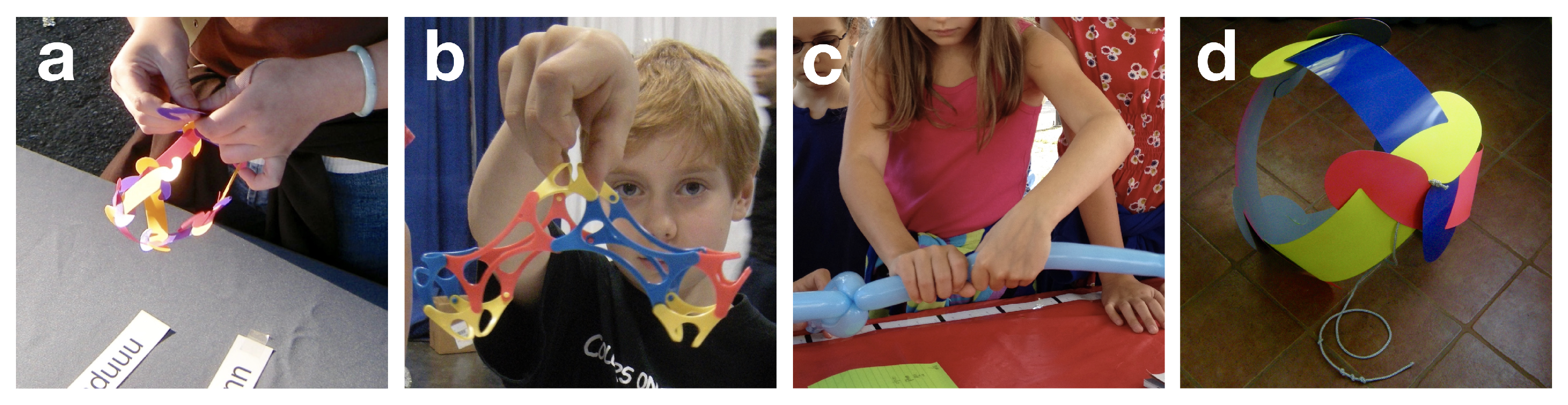
Some fun can be had making shapes this way. For example, I have done fair projects where participants learn to make a basket from a word (Figure 1a), or ‘evolve’ a new character sequence (via rewriting rules) and discover the shape that it describes by snapping pieces together (Figure 1b) or twisting balloons (Figure 1c). I have also made sculptures that include a description of their own shape, using a knotted string code inspired by the khipu codes of the Incas (Figure 1d).
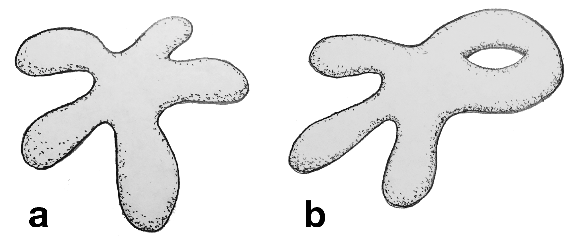
The codes I have used are able to describe the surfaces of branched three-dimensional objects, such as bushes or bodies with arms and legs—which are topological spheres (Figure 2a)—but not surfaces with a topological handle (Figure 2b). We will review, at some length, the coding and making of baskets without handles, and then show a limited way to extend these techniques to baskets with handles. This paper extends the work presented in [3].
2. Previous Work
There exists extensive literature on fabric construction and mathematics. The classic work of Grunbaum and Shephard [4,5,6,7] pioneered research into which periodic weaves are isonemal. Fabrics that are not isonemal are not really fabrics at all, as a set of warp and weft threads (that are themselves mutually interwoven) can lift off from the rest. Contemporary computer graphic research is interested in both modeling the appearance of fabrics and designing stitch meshes to cover a three-dimensional modeled surface [8,9,10,11,12,13]. There is also an active mathematical interest in ornamental Celtic knots which cover a meshed surface [14,15,16]. The work presented here assumes that the individual stitches–crochet stitches, net making knots, and interlocked weaving units–are secure enough individually that isonemality is not a practical worry, although a mathematical proof is lacking. This work, also, has a distinctly different goal from most computer graphics research relating to fabrics: We are not trying to fit a fabric to a form, rather we are curious to see what forms emerge spontaneously from a simple formal language that describes fabrics.
3. Background: Coding and Making Baskets without Handles
3.1. Preliminaries
Mullin [17], in 1967, described an encoding of graph drawings that has proved useful for coding the construction of fabric surfaces. His interest was counting graphs drawn on the surface of the sphere. Informally, a graph drawing [18], on a closed surface, is a connected drawing consisting of dots (0-dimensional vertices) connected by non-crossing curves (1-dimensional edges,) such that the regions left unmarked (2-dimensional faces) are simply connected. Considered up to topological equivalence, graph drawings on closed surfaces are maps. Informally, maps comprise all of the topologically distinct ways a closed surface can be cut up into polygons; conversely, they comprise all the topologically distinct ways polygons can be glued edge-to-edge to build closed surfaces.
All surfaces considered here will be orientable and, in fact, endowed with an orientation that gives words like ‘left’ and ‘counterclockwise’ unambiguous meanings. All surfaces are initially closed (i.e., boundary-less), though artificial boundaries or cuts may be later introduced, to render the surface into a topological polygon.
I emphasize that the surfaces are completely closed: They lack any opening that might be useful in serving the traditional functions of baskets. Every part of a fabric structure has many small openings that are characteristic of its fabric technique and, hence, it is simpler and more efficient to describe a useful functional opening in a basket as an extra-large characteristic opening in the fabric structure—that is, as an extra-large n-gon in the tessellation of the surface that describes the fabric structure—rather than as a boundary in the surface. The former approach not only simplifies the surface topology, it guarantees that the functional opening is properly salvaged in the fabric technique being used.
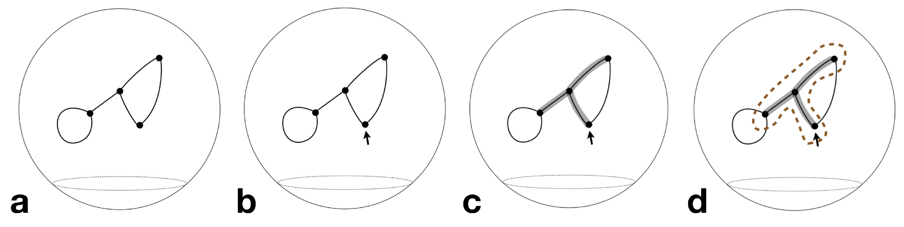
Mullin’s project was counting tree-rooted plane graphs (Figure 3). ‘Plane graph’ is synonymous with ‘graph drawing on the sphere’. A tree is a connected graph without cycles. A spanning tree of a graph is a tree which is a subset of the graph containing all of the vertices of the graph. One roots a graph drawing by distinguishing one of its corners—that is, a root face together with a root vertex—by drawing a small arrow in the root face pointing toward the root vertex. By convention, the corner’s edge closest (counterclockwise) to the rooting arrow is the root edge. By tree-rooted we mean that a graph drawing has been endowed with both a distinguished corner and a distinguished spanning tree. (Tree rooting gives the encoding algorithm a place to start, a direction to go in, and, as we will see, a complete ordering of the vertices and edges.)
3.2. Mullin’s Encoding
Mullin’s encoding algorithm ([18], p. 12) (see Figure 3d) begins at the root vertex and proceeds counterclockwise around a closed contour that wraps closely around the spanning tree. Walking around the contour, starting from where the rooting arrow intersects it, we will cross, and then re-cross, non-tree edges; and go along, then go back along, tree edges. These encounters are recorded in a character string, using two different styles of parentheses: ‘(’ records a crossing, ‘)’ records a re-crossing, ‘[’ records going out along an edge, and ‘]’ records going back along an edge.
The encoding tour in Figure 3d produces a shuffled parenthesis word: ‘([[)][()]]’. The parentheses of each style are, in relation to their own kind, properly nested, but the two different styles interleave freely. In this sense, two distinct systems of parentheses have been shuffled.
Maps have become central to current work in a wide range of fields [19]: Number theory, economics, and theoretical physics, among others. Mullin’s encoding easily converts a map on the sphere into a character string; effectively, an algebraic expression.
3.3. Mullin’s Decoding
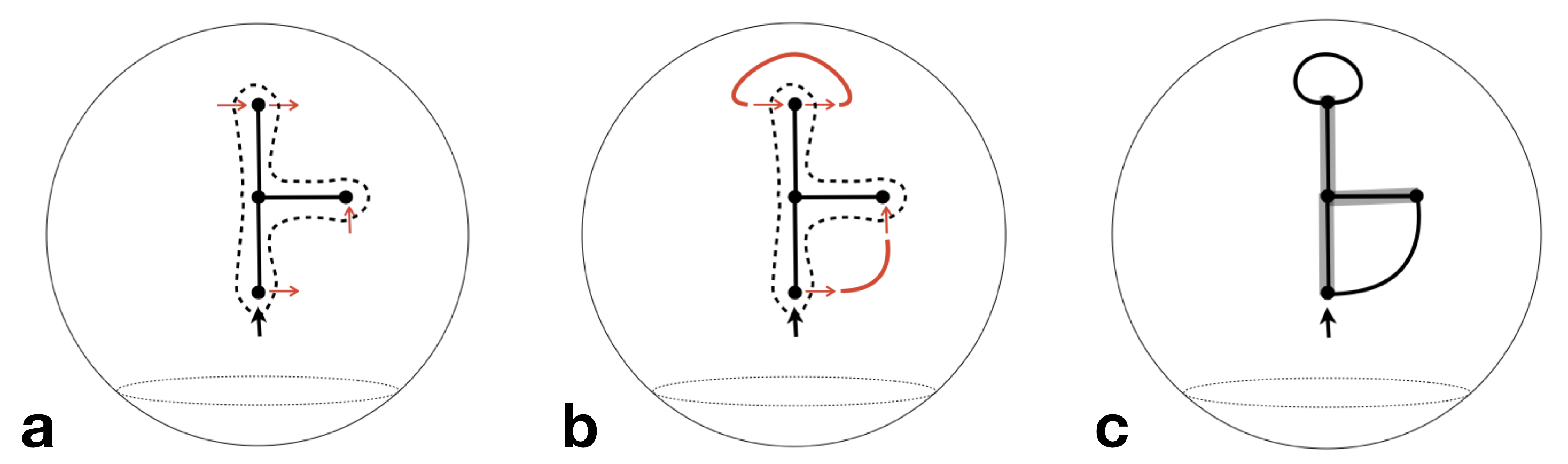
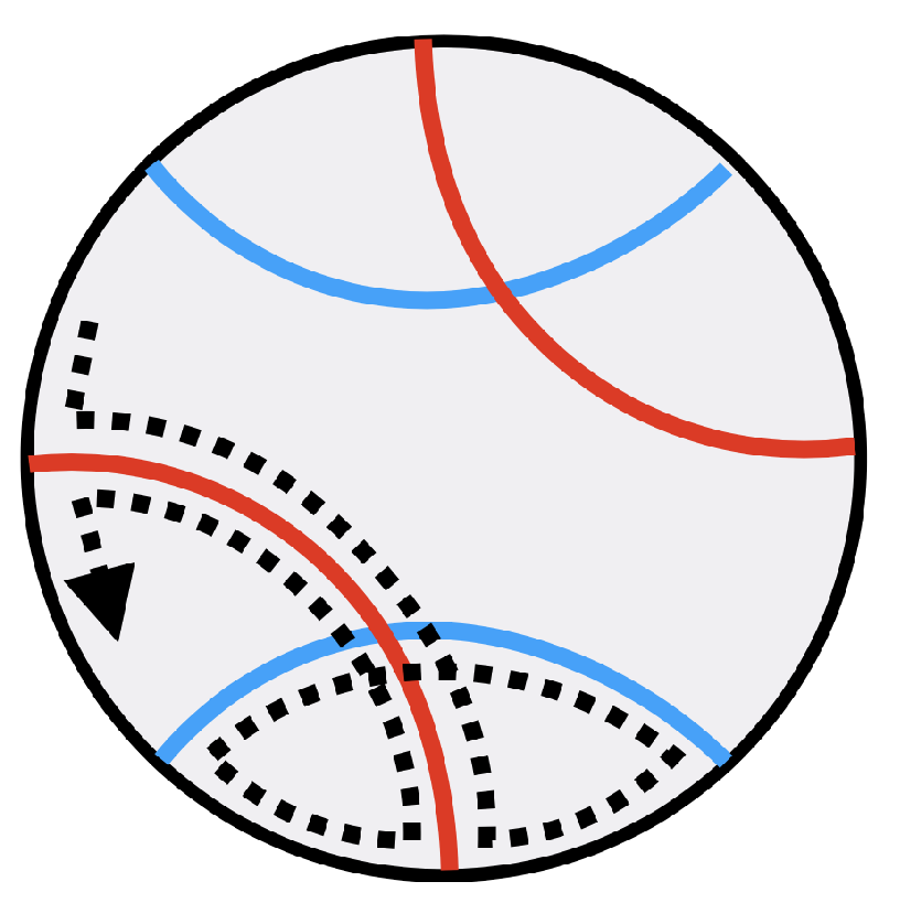
The tree-rooted plane graph can be recovered from its Mullin code through a sketching technique. Moving counterclockwise around the tree, we are in the process of sketching (see the dashed trajectory in Figure 4a), starting at a location that will become the root vertex: ‘[’ indicates to “draw an edge”; ‘]’ indicates to “move along the back side of an edge already drawn”; ‘(’ indicates to “decorate the current vertex with an outward arrow”; abd ‘)’ indicates to “decorate the current vertex with an inward arrow”. On a second lap around the tree, complementary arrows are connected, to recover the non-tree edges (the red lines in Figure 4b). The same rule used in algebra to pair up parentheses, “last opened, first closed" is used to pair up outward and inward arrows. (This sketching technique is not used in basket making, rather each of the four characters is interpreted as a craft action—execution of the fabric technique does the decoding).
In addition to a tree-rooted plane graph (Figure 5a), a Mullin code can also be interpreted as a 3-regular plane graph with a rooted Hamiltonian circuit (Figure 5b), or a 4-regular plane graph with a rooted A-trail (Figure 5c). An A-trail is a non-crossing Eulerian circuit comprised exclusively of hard-right and/or hard-left turns. [20,21] In the Hamiltonian circuit interpretation, the Mullin contour is the circuit, non-tree edges become the outer non-Hamiltonian edges, and the perpendiculars of tree edges become the inner non-Hamiltonian edges. In the A-trail interpretation, the non-Hamilton edges of the previous interpretation shrink to zero length, turning the Hamilton circuit into the edges of a 4-regular map with vertices located at the centers of the original map’s edges.
3.4. Mullin Encoding as a Formal Language
A formal language is a subset of all the character strings (or words) that can be spelled with a finite set of characters, , called its alphabet. Just as every set contains the null set, , every formal language contains the empty word, , the unique word of zero length. Typically, a formal language is an infinite subset, and its membership is defined by rewriting rules which suffice to generate all the words in the language (and only those words). For example, for , the Dyck language, = {(, )}, and the superset of all strings that can be spelled with those two characters is designated . The Dyck language, , is then the subset of consisting of all words, and only those words, that can generated from via the following rewriting rule (informally stated):
Insert a matched pair of parentheses, ‘()’, anywhere.
This one rule suffices to construct any balanced system of parentheses—such as would be meaningful in a mathematical expression—and only such systems. For example: → () → ()() → (())().
Viewed as a formal language, Mullin’s encoding is , the shuffled Dyck language on two types of parenthesis [22]. Words in are shuffles of two words, each word having its own parenthesis style, so = {(, ), [, ]}. is the subset of consisting of all words, and only those words, that can generated from via the following rewriting rules (informally stated):
Insert a matched pair of parentheses, ‘()’ or ‘[]’, anywhere.
Shuffle adjacent parentheses of unlike style past each other, e.g., []()→[(]).
For example, to obtain the word ([)]: → () → ([]) → ([)].
In my experience, given some one-on-one instruction, even very young children can master these rules to sequentially write down or ‘evolve’ their own codes for baskets. To make the game easier, I map the alphabet, {(, ), [, ]}, to {u, d, n, p}, and call the language undip [1]. The shape of each letter in undip has a mnemonic connotation of open/close, and (when read with the head leaning to the right) a connotation of left/right, so that the basket maker escapes memorizing the translation.
The rewriting rules allow us to generate an word inside or beside another word—the same being true of —so, and words have the rather DNA-like property that they can be freely concatenated or spliced into one another. The formal language underpins what is interesting about Mullin’s code from a sculptural—or playful—point of view: Design can be accomplished by an accumulation of essentially random local mutations.
Via Mullin’s encoding, allows us to generate any map on the sphere as the consequence of a ‘word game’, and, therefore, as we will see below, to make a basket that exemplifies that map. If the fabric technique allows local edits to be made in an otherwise finished shape, a metamorphosis is possible simply by traveling repeatedly around the same Mullin contour, making local insertions and shuffles as the occasion arises. This could be a practical method of ‘growing’ shapes in fabric systems, such as tensegrity, that are weak or disorganized when the structure is in an unfinished state.
As an aside, formal languages are closely related to abstract algebra and group theory. For example, the operation of string concatenation is associative and closed on any , and is its identity element; thus, , under string concatenation, is a monoid, lacking only inverses to constitute a group. This is why is sometimes referred to as the free monoid on . A congruence relation then supplies the role of the rewriting rules, restricting the free monoid to a submonoid, which corresponds to some formal language. For example, if the binary operation is a non-commutative multiplication, the relation gives an algebraicist license to make the following derivation: …, and so on, which is, of course, an analog of the generation of a word in by the insertion rule. Adding the relation allows a second style of parenthesis, which requires. Adding the four relations , , , and justifies invocations of the shuffle rule in deriving words of . For example: . In the totality of such derivations, the equivalence class of 1 becomes the analog of . Deriving baskets might be an interesting way for students to interact with algebra and group theory.
3.5. Shuffled Dyck Words Describe Constrained Lattice Walks
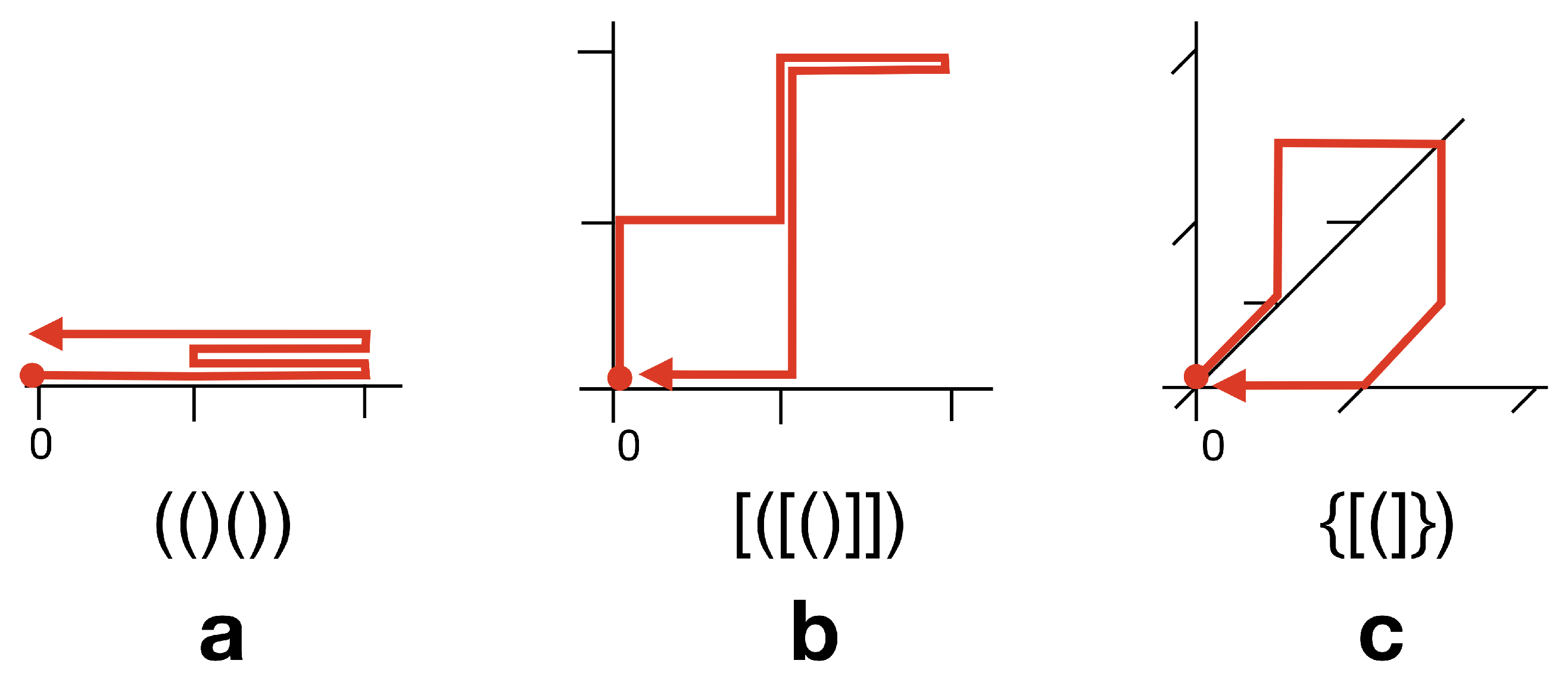
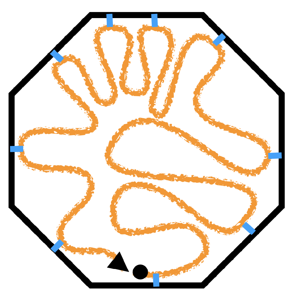
Strings of shuffled parentheses are hard to read and interpret, so the following visualization is often helpful. A word in can be seen as describing a constrained walk on the n-dimensional lattice, beginning and ending at the origin (Figure 6). Each style of parenthesis gets its own coordinate axis: An open parenthesis increments its coordinate, a close parenthesis decrements it. For example, a word in the Dyck language () describes an origin-to-origin walk, constrained to the positive half of the integer numberline (the 1D lattice); a word in describes an origin-to-origin walk constrained to the first quadrant of the 2D lattice; a word in (which we will have use for later) describes an origin-to-origin walk constrained to the first octant of the 3D lattice. For these examples, walks of steps (e.g., words of letters) are enumerated, respectively [23,24,25], by the kth Catalan number; , the product of consecutive Catalan numbers (This enumeration is not hard to calculate, but it proved for a long time hard to explain [26], because it implied an undiscovered bijection between words in and concatenations of two words in ), ; and the OEIS integer sequence A064037.
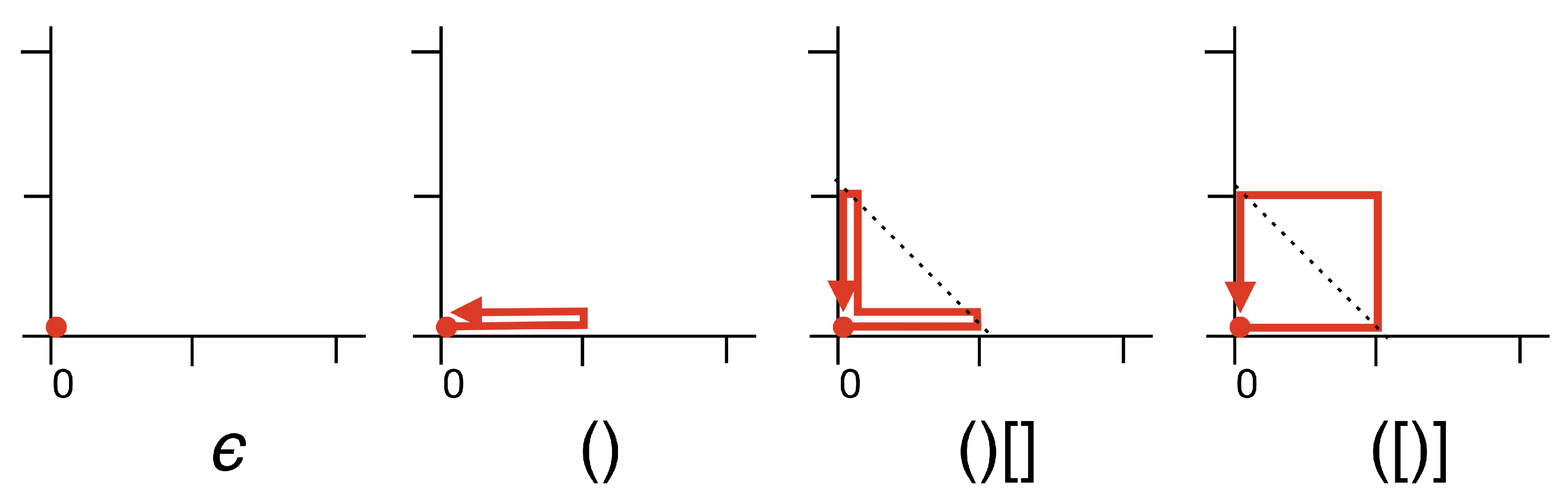
The insertion and shuffle rewriting rules can also be considered, in terms of a lattice walk (Figure 7). An insertion move appears as an out-and-back spike directed away from the origin. Neighboring parentheses of unlike style appear as 90-degree corners. A shuffle move folds or unfolds the corner, diagonally.
3.6. Bijections between Maps and Baskets
A bijection is an invertible mapping. Invertibility establishes that no information is lost in the mapping, justifying the view that object and image are merely different representations for the same underlying object. Schaeffer [18] described a bijection from maps with n edges onto face bicolored 4-regular maps with n vertices, which he termed edge maps. (Uncolored, the same maps are known elsewhere as medial maps; in relation to polyhedra, the transformation is known as an ambo or rectification).
Definition 1.
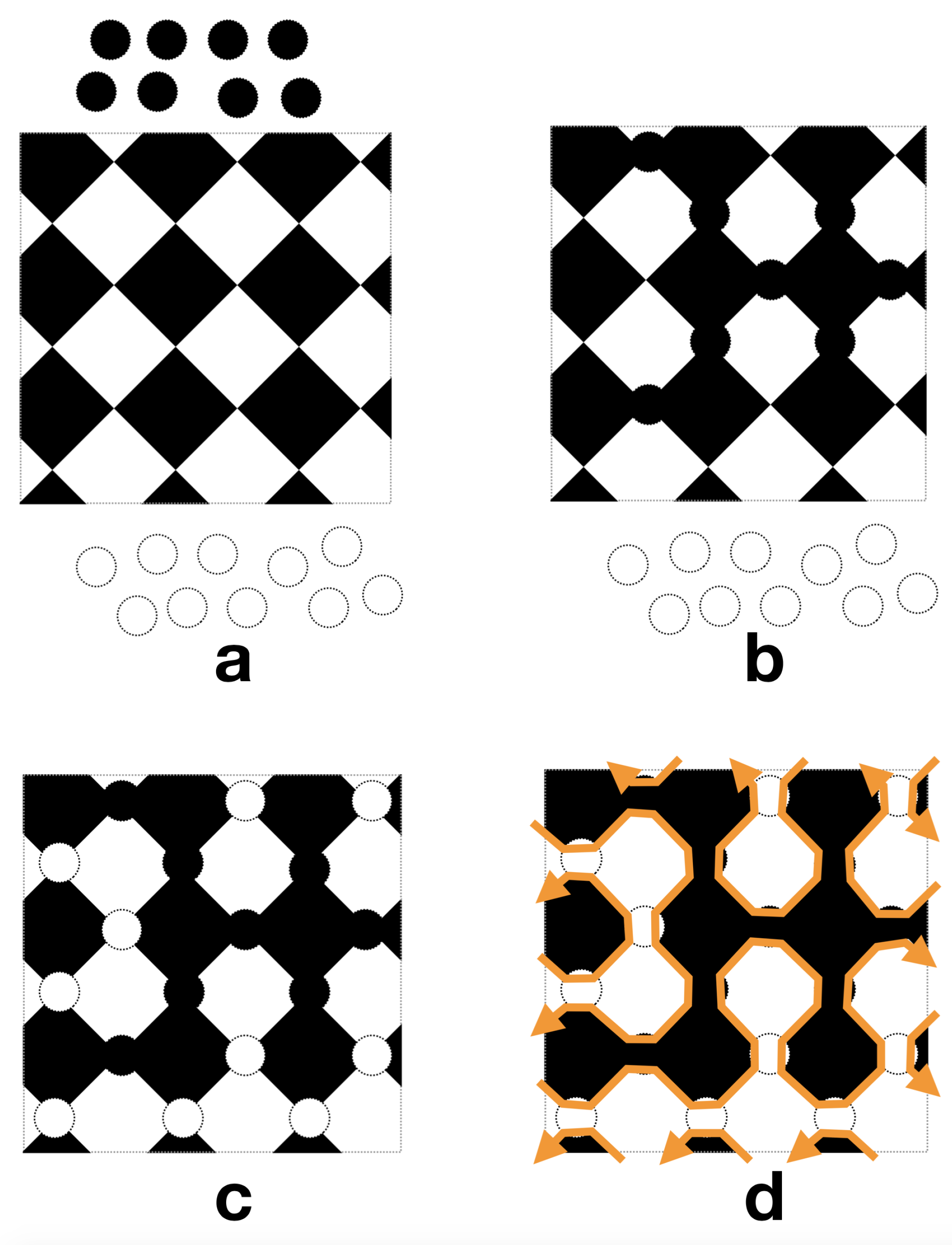
An edge map that is face bicolored, in accordance with the following natural visualization, of the maps-to-edge-maps bijection is a basket map: Given a map that is visualized as a black graph drawn on a white surface (Figure 8a), enlarge the black dots that represent the vertices until they meet at the middle of the now obscured edges (Figure 8b).
A basket map is like a checkerboard, in that black regions (the vertex images) and white regions (the face images) meet at four-cornered intersections (the edge images), with the colors alternating black-white-black-white around the intersection. A basket map is unlike a checkerboard, in that the colored regions are not necessarily quadrilateral—they may have any number of sides. To visualize the inverse mapping from a basket map to a map: Shrink the black regions of a basket map (Figure 8b) away from their four-cornered intersections, leaving only a thread of black behind (Figure 8a).
Use of the term ‘basket’ is justified by the fact that a face-bicolored 4-regular map is an alternating projection of a link; in effect, a projection of a plain-woven basket [27,28] (i.e., a basket woven in a strictly over-under-over-under pattern). The invertible mapping from a basket map to a plain-woven basket is summarized as follows: A weaver, standing in a region that is black in the basket map (Figure 8b), sees herself in the plain-woven basket (Figure 8c) surrounded by right-over-left weave crossings (conversely, left-over-right when standing in a white region). A physical model of Figure 8c (e.g., a belt given a full counterclockwise twist before being buckled) helps to verify that the weave crossings surrounding a region of a given color have the same appearance, regardless of whether the observer is standing on the ‘outside’ or ‘inside’ of the surface—orientation reversal introduces no difficulty in translating a basket map into a plain-woven basket.
An important property of this chain of bijections is that the map dual-images to the opposite coloring of the basket map and, thus, in the plain woven basket, is merely the opposite handedness of weaving.
3.7. Fabric Construction
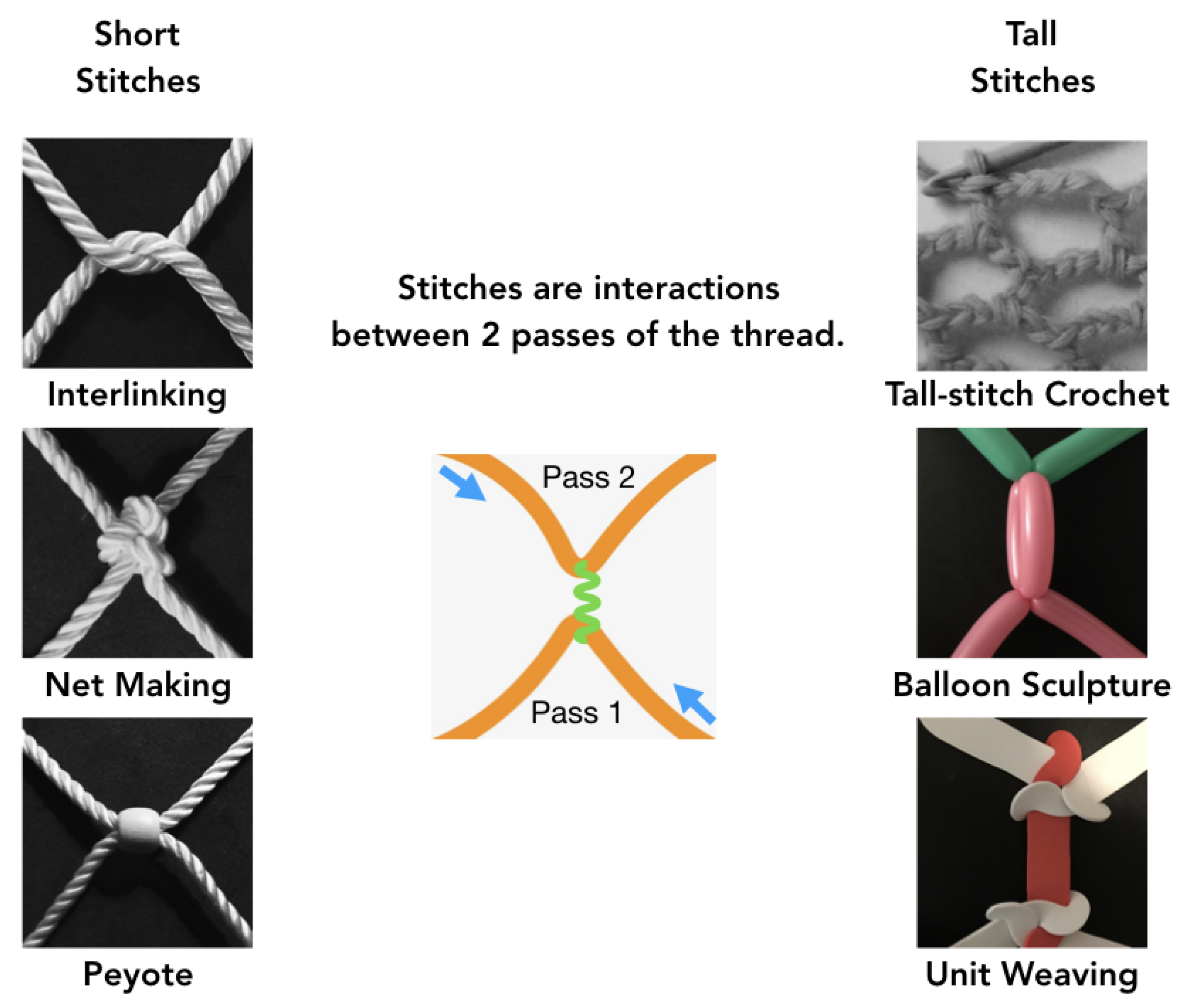
A Mullin code describes, by the bijections above, the finished structure of a plain-woven basket—unfortunately, weaving is hard. Making a basket by weaving is more complex than making it by a single thread technique, such as net making. Except for unit weaving (see the lower right panel of Figure 9), a simplified version of weaving where the weaving elements are made as short as possible, finding a working order for weaving will be beyond the scope of this paper. Watching a basket weaver work with dozens of strands in action at once may convince one of this point; the practical necessity of splices is another complication. Rather, we have introduced basket maps, here, because they also elegantly describe those fabric techniques (Figure 9) where the thread turns away after each interaction rather than continuing straight and crossing over. In other words, instead of following the straightest-possible path through the basket map, the thread follows a maximally-crooked path through the basket map: A sequence of hard-right or hard-left turns. The mathematical term for such a course is an A-trail, perhaps so-called because each turn of the trail can be indicated on the map by drawing a little shortcut reminiscent of the horizontal stroke in the letter ‘A’. Figure 5c shows an example of an A-trail on a 4-regular map.
We are therefore interested in finding the progressive course of a single thread which builds a surface by interacting with itself at the turns of an A-trail. This problem on the sphere is subsumed by the general case considered below, so we will proceed now to our main object.
4. Coding Surfaces with Handles
4.1. Surfaces and Polygonal Schemata
One definition of a topological surface is a polygonal disk with sides identified in oriented pairs. The polygon, together with the oriented pairings of its sides, constitutes a polygonal schema for the surface. If all pairings are done without twisting, the result is an orientable surface; any such pairings will result in an orientable surface, and an orientable surface with any number of handles can be obtained in this way.
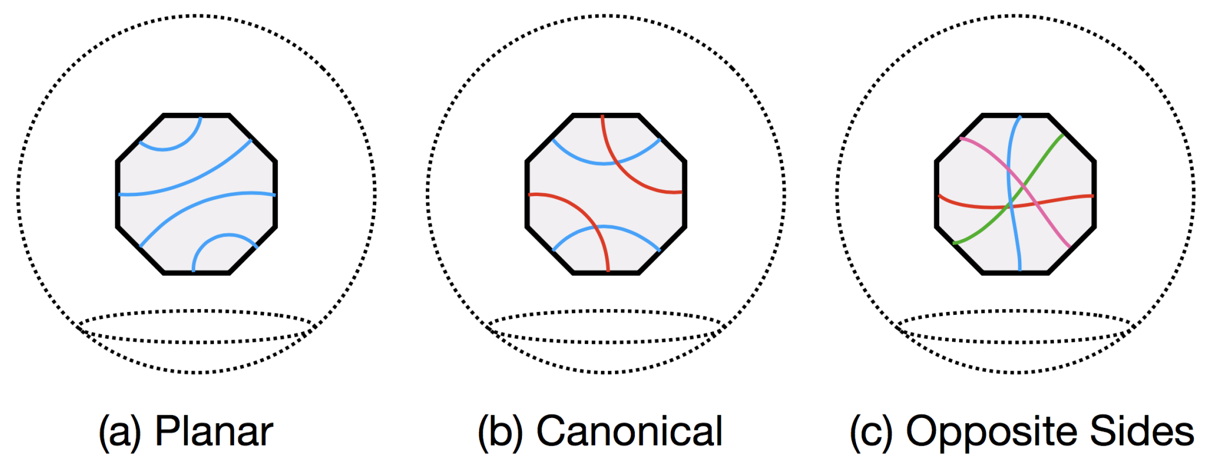
A polygonal schema can also be viewed as a spherical surface with a polygonal boundary (i.e., a polygonal hole). That these two viewpoints are equivalent can be driven home by imagining a polygonal disk enlarged to cover half of a geometric sphere. Then, the two alternate viewpoints are simply views from the convex and concave sides. Figure 10 shows this ‘backside view’ of three different polygonal schemata. The advantage of this perspective is that we can indicate the pairing of sides with short arcs, chords, drawn across the hole without obscuring or implying any interference with the fabric structure of the surface itself.
Gluing together the sides of a polygonal schema yields a 1-face map with n edges. This map is known as the cut graph. We can reverse the gluing procedure by making a razor cut along each edge of the cut graph and then pulling the resulting cuts open. It is, then, apparent that the backside view (Figure 10) is also a tailor’s view as he tries to stitch the cuts back up. The chords of the chord diagram are stitches that need to be made. Though they appear as long, crossing arcs, when the stitches are drawn tight to pull the surface back together, each stitch will contract to just a point on one of the edges of the cut graph.
Notice that, if we extrapolate the chords out onto the spherical surface without crossing, they must all meet at one vertex on the far side of the sphere. By that understanding, backside views of the polygonal schema also represent an abbreviated view of the 1-vertex map which is the dual of the cut graph. In particular, the dual map has 1 vertex, n edges, and faces whose edge cycles can traced (say, for counting purposes) directly on the chord diagram (Figure 11). This can be a convenient way to calculate the genus of the surface from its chord diagram, by using the formula for the Euler characteristic.
4.2. Fabric Construction within a Polygonal Schema
If the A-trail that the thread follows never crosses the cut graph (i.e., only interactions can cross it), then things are simple—we are just making a polygonal disk of fabric [29]. It turns out that this is always the case, as we will see below: An A-trail that covers a surface induces a cut graph that it does not cross [30]. So, the only problems introduced by baskets with handles are: Which segments of thread meet each other across the cut graph? Can our coding language specify these pairings?
As the A-trail is a simple closed loop, traversed in a counterclockwise direction (Figure 12), it can only touch the boundary of the polygonal disk in a strictly cyclical, counterclockwise order—note that the direction of progress will appear reversed in the backside view. Also, all interactions with the boundary lie on the outer (i.e., right) side of the trail. On a surface without a handle, all of the right-side interactions are coded with square brackets.
4.3. Extension to
If the chords in the schema can be drawn without crossings (Figure 10a), the polygonal opening closes up to a cut graph which is a tree, which shows that the surface is a topological sphere and can be coded in .
If any chords do cross, if we were to attempt to code the basket with just the one style of parenthesis for the right side, the crossed chords would be mis-wired when the current ‘close’ parenthesis is associated with the most recent ‘open’ parenthesis. We need at least two styles of parenthesis on the right side to disambiguate pairs of chords that cross. We add the curly brackets, ‘{’ and ‘}’, for this purpose. That extends to , the shuffled Dyck language on 3 types of parentheses, with the specification that one of the types of parenthesis (the round style) codes for the left side, and the other two (the square and curly styles) interchangeably code for the right.
can code surfaces with any number of handles, as is demonstrated by the fact that the chords of any canonical polygonal schema (see Figure 11b) can be 2-colored, such that chords of the same color do not cross. There is an word for any basket whose chord diagram is 2-colorable; and in fact, the right-side subword codes for the chord diagram, so the 2-D constrained lattice walks (Figure 6b) describe polygonal schemata, as well as spherical baskets.
Figure 13 shows an example of a basket worked in unit-weaving from the word [{[}[{]{]}]}. The absence of round parentheses indicates that the interior (left side) of the Hamiltonian circuit is a single face. The surface is difficult to visualize in this skeletal form, but it is easy to verify that it is indeed orientable, and has 12 vertices, 18 edges, and 4 faces. Counting of faces can be done directly on the code word by connecting paired parentheses with arches, and then viewing the arch diagram as a linear chord diagram that can be traced, as in Figure 11—note that a chord diagram with n chords always has . The Euler characteristic, , verifies that it is a double torus. The weaver of a higher genus basket needs an intuition of the intended imbedding in 3-space. For example, all of the mathematical knots would be potential weaving errors in a project to make a bagel-shaped basket, using surface data alone.
Unfortunately, some cut graphs have schemata that cannot be 2-colored (e.g., Figure 11c), and thus cannot be coded in . In playing the word game, we will hardly be aware of the chord diagrams we cannot describe, because they will never be spelled. Some other difficulties arise, however. Since exhaustively labels every possible way to 2-color the chord diagram, randomly generated words will intensively explore coloring variations we are probably not very interested in. There is also the human prejudice for low-genus surfaces. Canonical chord diagrams (Figure 11b), for example, need just two parentheses per handle and, thus, a random exploration of long words will spend a lot of time examining surfaces with a great many topological handles that may be as rudimentary as a pair of crossed threads.
4.4. Finding A-Trails on Higher Genus Surfaces
From a purely word-game point of view, we never need to find A-trails: We build them, as some newly-derived word in directs. However, often there are occasions where we wish to design a basket shape first, and then figure out a word that encodes it. This section restates some of [30], perhaps more concisely in terms of the basket map.
The Euler characteristic, , is a constant aid in dealing with higher genus maps:
where V is the number of vertices, E the number of edges, and F the number of faces.
One algorithm for finding a spanning tree (a submap containing all the vertices of the original map, but no cycles) is to start with one vertex and then iteratively add an adjacent edge that reaches a new vertex. Starting from one face and one vertex, each step adds one edge, one vertex, and no faces; so, remains constant at 2—any tree is a spherical map. As the initial vertex was gained without an edge, every tree has one more vertex than edges, .
The genus, g (equivalently, the number of handles), is related to the Euler characteristic by:
Equations (1) and (2) combine to:
However, is the number of edges, , in any spanning tree of the primal map, and is the number of edges, , in any spanning tree of the dual map; therefore, we have an expression of Euler’s relation that (overtly, at least) only counts edges:
In words, the number of edges in any map is equal to the number of edges in a spanning tree, plus the number of edges in a spanning tree of its dual, plus 2 edges per handle.
What corresponds, in the dual map, to the iterative construction of a spanning tree in the primal? The dual map has the Euler characteristic of the surface. The singleton vertex that starts the spanning tree appears as a single face in the dual. If we delete from the dual the image of the edge that is added to the tree in the primal, we will amalgamate two of the dual’s faces into one. Each iterated step reduces the number of edges in the dual by one, faces by one, and leaves the vertices unchanged; so, remains unchanged. The growing tree eventually connects all the vertices in the primal map, and all of the faces of the dual map are eventually amalgamated into one face. The spanning tree on the primal map, thus, induces a one-face map, called a g-tree in [30], that still represents the surface. By Equation (4), the number of edges in the g-tree is exactly the minimum needed to connect all its vertices, plus two edges per topological handle. Any g-tree is a cut graph, but usually one with many more cuts than are strictly necessary from a topological point of view. An analogy would be mapping the coastline of a volcanic island: Should we include the shores of creeks that drain the interior to the sea? A reduced g-tree, what one would more typically think of as a cut graph, can be obtained by iteratively removing 1-valent vertices (and their single attached edges) until no more are left. The spanning tree and the unreduced g-tree form a labyrinth that permits only one traversal (an A-trail) of the medial graph. These relations are unified in the basket map.
4.5. Finding A-Trails with a Board Game on the Basket Map
Expressing Euler’s characteristic in variables native to basket maps: Vertices correspond to black regions (B), edges correspond to intersections (I), and faces correspond to white regions (W),
The edge relation, Equation (4), becomes:
Figure 14 is a basket map corresponding to a braided torus; opposite sides of the rectangle are to be identified. We can indicate addition of an edge to the spanning tree by covering the corresponding intersection in the basket map with a black checker. After black (primal) has marked the entire spanning tree in this way (and thus, all the black regions are simply connected), using up all black checkers in the process, we allow white (dual) to claim all the remaining intersections by placing white checkers on them, using up all white checkers in the process. The black/white boundary in the checker-covered basket map is, now, an A-trail that visits the entire surface.
To ensure that the game ends in an A-trail that can be encoded in , we should allow white to play first, marking a suitable cut-graph with white checkers; black can then build its spanning tree; then white can claim the remaining intersections. The numbers of black and white checkers are the same, when the game is played this way.
5. Conclusions and Future Directions
I have shown that Mullin’s 4-character encoding of tree-rooted plane graphs—which corresponds to mathematical abstractions of fabric construction—can be extended to orientable surfaces with handles, provided we are free to make an advantageous choice of the polygonal schema.
My hope is that this extended code might have some of the ‘DNA’-like properties of , for experiments in ‘genetic engineering’ of baskets with handles. A clear line of research is in finding a geometric characterization of cut graphs whose chord diagrams are 2-colorable.
Funding
This research received no external funding.
Acknowledgments
The author is grateful for a reviewer’s assistance in finding relevant citations in this field of research.
Conflicts of Interest
The author declares no conflict of interest.
References
- Mallos, J. Evolve Your Own Basket. In Proceedings of Bridges 2012: Mathematics, Music, Art, Architecture, Culture; Robert Bosch, D.M., Sarhangi, R., Eds.; Tessellations Publishing: Phoenix, AZ, USA, 2012; pp. 575–580. Available online: http://archive.bridgesmathart.org/2012/bridges2012-575.html (accessed on 10 December 2018).
- Mallos, J. DNA-inspired Basketmaking: Scaffold-Strand Construction of Wireframe Sculptures. In Proceedings of Bridges 2017: Mathematics, Art, Music, Architecture, Education, Culture; David Swart, C.H.S., Fenyvesi, K., Eds.; Tessellations Publishing: Phoenix, AZ, USA, 2017; pp. 57–62. Available online: http://archive.bridgesmathart.org/2017/bridges2017-57.pdf (accessed on 10 December 2018).
- Mallos, J. Walking Around Trees: A 6-Letter ‘DNA’ for Baskets with Handles. In Proceedings of Bridges 2018: Mathematics, Art, Music, Architecture, Education, Culture; Torrence, E.T.B., Séquin, C., Fenyvesi, K., Eds.; Tessellations Publishing: Phoenix, AZ, USA, 2018; pp. 219–224. Available online: http://archive.bridgesmathart.org/2018/bridges2018-219.pdf (accessed on 10 December 2018).
- Grunbaum, B.; Shephard, G. Satins and twills: An introduction to the geometry of fabrics. Math. Mag. 1980, 53, 139–161. [Google Scholar] [CrossRef]
- Grunbaum, B.; Shephard, G. A catalogue of isonemal fabrics. Ann. N. Y. Acad. Sci. 1985, 440, 279–298. [Google Scholar] [CrossRef]
- Grunbaum, B.; Shephard, G. An extension to the catalogue of isonemal fabrics. Discret. Math. 1986, 60, 155–192. [Google Scholar] [CrossRef] [Green Version]
- Grunbaum, B.; Shephard, G. Isonemal fabrics. Am. Math. Mon. 1988, 95, 5–30. [Google Scholar] [CrossRef]
- Narayanan, V.; Albaugh, L.; Hodgins, J.; Coros, S.; McCann, J. Automatic machine knitting of 3D meshes. ACM Trans. Graph. (TOG) 2018, 37, 35. [Google Scholar] [CrossRef]
- Yuksel, C.; Kaldor, J.M.; James, D.L.; Marschner, S. Stitch meshes for modeling knitted clothing with yarn-level detail. ACM Trans. Graph. (TOG) 2012, 31, 37. [Google Scholar] [CrossRef]
- Wu, K.; Gao, X.; Ferguson, Z.; Panozzo, D.; Yuksel, C. Stitch meshing. ACM Trans. Graph. (TOG) 2018, 37, 130. [Google Scholar] [CrossRef]
- Akleman, E.; Chen, J.; Chen, Y.; Xing, Q.; Gross, J.L. Cyclic twill-woven objects. Comput. Graph. 2011, 35, 623–631. [Google Scholar] [CrossRef]
- Akleman, E.; Chen, J.; Gross, J.L. Extended graph rotation systems as a model for cyclic weaving on orientable surfaces. Discret. Appl. Math. 2015, 193, 61–79. [Google Scholar] [CrossRef] [Green Version]
- Xing, Q.; Esquivel, G.; Collier, R.; Tomaso, M.; Akleman, E. Spulenkorb: Utilize Weaving Methods in Architectural Design. In Proceedings of Bridges 2011: Mathematics, Music, Art, Architecture, Culture; Tessellations Publishing: Phoenix, AZ, USA, 2011; pp. 163–170. [Google Scholar]
- Kaplan, M.; Cohen, E. Computer Generated Celtic Design. In Proceedings of the 14th Eurographics Workshop on Rendering, ACM Siggraph, Leuven, Belgium, 25–27 June 2003; pp. 9–16. [Google Scholar]
- Kaplan, M.; Praun, E.; Cohen, E. Pattern oriented remeshing for Celtic decoration. In Proceedings of the Pacific Graphics 2004, Seoul, Korea, 6–8 October 2004; pp. 199–206. [Google Scholar]
- Mercat, C. Les entrelacs des enluminure Celtes. Doss. Pour Sci. 2001, 15. Available online: http://www.academia.edu/18455479/Les_entrelacs_des_enluminures_celtes (accessed on 10 December 2018).
- Mullin, R.C. On the enumeration of tree-rooted maps. Can. J. Math. 1967, 19, 174–183. [Google Scholar] [CrossRef]
- Schaeffer, G. Planar maps. Handb. Enumer. Comb. 2015, 87, 335. [Google Scholar]
- Lando, S.K.; Zvonkin, A.K. Graphs on Surfaces and Their Applications; Springer Science & Business Media: Berlin, Germany, 2013; Volume 141. [Google Scholar]
- Fleischner, H. Eulerian Graphs and Related Topics; Elsevier: Amsterdam, The Netherlands, 1990; Volume 1. [Google Scholar]
- Benson, E.; Mohammed, A.; Gardell, J.; Masich, S.; Czeizler, E.; Orponen, P.; Högberg, B. DNA rendering of polyhedral meshes at the nanoscale. Nature 2015, 523, 441. [Google Scholar] [CrossRef] [PubMed]
- Cori, R.; Dulucq, S.; Viennot, G. Shuffle of parenthesis systems and Baxter permutations. J. Comb. Theory Ser. A 1986, 43, 1–22. [Google Scholar] [CrossRef]
- The On-Line Encyclopedia of Integer Sequences. OEIS A000108. Available online: https://oeis.org/A000108 (accessed on 10 December 2018).
- The On-Line Encyclopedia of Integer Sequences. OEIS A005568. Available online: https://oeis.org/A005568 (accessed on 10 December 2018).
- The On-Line Encyclopedia of Integer Sequences. OEIS A064037. Available online: https://oeis.org/A064037 (accessed on 10 December 2018).
- Bernardi, O. Bijective counting of tree-rooted maps and shuffles of parenthesis systems. Electron. J. Comb. 2007, 14, 9. [Google Scholar]
- Akleman, E.; Chen, J.; Xing, Q.; Gross, J.L. Cyclic plain-weaving on polygonal mesh surfaces with graph rotation systems. ACM Trans. Graph. (TOG) 2009, 28, 78. [Google Scholar] [CrossRef]
- Roelofs, R. About Weaving and Helical Holes. In Proceedings of Bridges 2010: Mathematics, Music, Art, Architecture, Culture; Hart, G.W., Sarhangi, R., Eds.; Tessellations Publishing: Phoenix, AZ, USA, 2010; pp. 75–84. Available online: http://archive.bridgesmathart.org/2010/bridges2010-75.html (accessed on 10 December 2018).
- Belcastro, S.M. Every topological surface can be knit: A proof. J. Math. Arts 2009, 3, 67–83. [Google Scholar] [CrossRef]
- Chapuy, G.; Marcus, M.; Schaeffer, G. A bijection for rooted maps on orientable surfaces. SIAM J. Discret. Math. 2009, 23, 1587–1611. [Google Scholar] [CrossRef]
Figure 1.
Fun with building shapes from code: (a) “Make a basket from a word”, (b) “Evolve a basket”, (c) “Evolve your own balloon animal”, (d) “Knots code shapes”.
Figure 1.
Fun with building shapes from code: (a) “Make a basket from a word”, (b) “Evolve a basket”, (c) “Evolve your own balloon animal”, (d) “Knots code shapes”.

Figure 2.
Closed baskets whose surfaces have: (a) Zero handles, (b) one handle.

Figure 3.
Tree-rooted plane graphs: (a) A plane graph, (b) a rooted plane graph, (c) a tree-rooted plane graph, (d) Mullin’s encoding of a tree-rooted plane graph: Starting from the root arrow and proceeding counterclockwise around the dashed contour, the encoding is ‘([[)][()]]’.
Figure 3.
Tree-rooted plane graphs: (a) A plane graph, (b) a rooted plane graph, (c) a tree-rooted plane graph, (d) Mullin’s encoding of a tree-rooted plane graph: Starting from the root arrow and proceeding counterclockwise around the dashed contour, the encoding is ‘([[)][()]]’.

Figure 4.
Mullin’s decoding: (a) Begin at what will be the root vertex, work in a counterclockwise circuit. Square parentheses direct drawing tree edges or moving along tree edges already drawn, and round parentheses direct decorating vertices with outward or inward arrows; (b) complementary arrows pair up to form the non-tree edges; and (c) the recovered tree-rooted plane graph.

Figure 5.
Alternate interpretations. A Mullin code describes: (a) A tree-rooted plane graph, (b) a 3-regular plane graph with a rooted Hamiltonian circuit, or (c) a 4-regular plane graph with a rooted A-trail, or non-crossing Eulerian circuit.
Figure 5.
Alternate interpretations. A Mullin code describes: (a) A tree-rooted plane graph, (b) a 3-regular plane graph with a rooted Hamiltonian circuit, or (c) a 4-regular plane graph with a rooted A-trail, or non-crossing Eulerian circuit.

Figure 6.
words as lattice walks: (a) A word in the Dyck language, , describes an origin-to-origin walk on the positive half of the integer numberline (1D lattice); (b) a word in describes an origin-to-origin walk in the first quadrant of the 2D lattice; and (c) a word in describes an origin-to-origin walk in the first octant of the 3D lattice.

Figure 7.
Derivation of the word ‘([)]’, viewed as an evolving lattice walk. An insertion move shows as an out-and-back spike directed away from the origin. Neighboring parentheses of unlike style show up as a 90-degree corner. Making a shuffle move folds or unfolds the corner, diagonally.
Figure 7.
Derivation of the word ‘([)]’, viewed as an evolving lattice walk. An insertion move shows as an out-and-back spike directed away from the origin. Neighboring parentheses of unlike style show up as a 90-degree corner. Making a shuffle move folds or unfolds the corner, diagonally.

Figure 8.
Bijections connecting maps to plain woven baskets: (a) A graph drawing on a closed surface, a map; (b) the black vertex dots of the map are enlarged until they meet at the middle of the obscured edges, a basket map; and (c) a plain-woven basket, woven according to the basket map—standing in a black region of the basket map, the weaver sees the surrounding weave crossings as right-over-left.

Figure 9.
Examples of fabric techniques that can be abstracted as an A-trail on the basket map.

Figure 10.
Backside (or chord diagram) views of three polygonal schemata: (a) A planar schema; (b) a canonical schema; and (c) a schema where opposite sides are identified.
Figure 10.
Backside (or chord diagram) views of three polygonal schemata: (a) A planar schema; (b) a canonical schema; and (c) a schema where opposite sides are identified.

Figure 11.
Tracing, on the chord diagram, a face of the cut graph’s dual: In this diagram, there is only 1 face, so the Euler characteristic is The surface is a double torus.
Figure 11.
Tracing, on the chord diagram, a face of the cut graph’s dual: In this diagram, there is only 1 face, so the Euler characteristic is The surface is a double torus.

Figure 12.
Frontside view of a polygonal schema with a simple closed loop traced in a counterclockwise direction—the loop can only touch the bounding polygon in a strictly counterclockwise, cyclical order, and only on its outer (or right) side.
Figure 12.
Frontside view of a polygonal schema with a simple closed loop traced in a counterclockwise direction—the loop can only touch the bounding polygon in a strictly counterclockwise, cyclical order, and only on its outer (or right) side.

Figure 13.
A unit-woven double torus with the code word [{[}[{]{]}]}. Hamiltonian circuit in green.

Figure 14.
The game of finding an A-trail on a basket map: (a) A torus basket map with , , and ; (b) state of play after black has connected all B black regions with his chips; (c) final state of play after white has claimed the remaining intersections using all of her chips; and (d) the oriented A-trail that follows the black/white boundary, with black on the left.

© 2019 by the author. Licensee MDPI, Basel, Switzerland. This article is an open access article distributed under the terms and conditions of the Creative Commons Attribution (CC BY) license (http://creativecommons.org/licenses/by/4.0/).
Share and Cite
MDPI and ACS Style
Mallos, J. A 6-Letter ‘DNA’ for Baskets with Handles. Mathematics 2019, 7, 165. https://doi.org/10.3390/math7020165
AMA Style
Mallos J. A 6-Letter ‘DNA’ for Baskets with Handles. Mathematics. 2019; 7(2):165. https://doi.org/10.3390/math7020165
Chicago/Turabian StyleMallos, James. 2019. "A 6-Letter ‘DNA’ for Baskets with Handles" Mathematics 7, no. 2: 165. https://doi.org/10.3390/math7020165
Note that from the first issue of 2016, this journal uses article numbers instead of page numbers. See further details here.