Exact Algorithms for Maximum Clique: A Computational Study

Computing Science, University of Glasgow, Glasgow G12 8QQ, UK
Algorithms 2012, 5(4), 545-587; https://doi.org/10.3390/a5040545
Submission received: 11 September 2012
/
Revised: 29 October 2012
/
Accepted: 29 October 2012
/
Published: 19 November 2012
(This article belongs to the Special Issue Graph Algorithms)
Abstract
:We investigate a number of recently reported exact algorithms for the maximum clique problem. The program code is presented and analyzed to show how small changes in implementation can have a drastic effect on performance. The computational study demonstrates how problem features and hardware platforms influence algorithm behaviour. The effect of vertex ordering is investigated. One of the algorithms (MCS) is broken into its constituent parts and we discover that one of these parts frequently degrades performance. It is shown that the standard procedure used for rescaling published results (i.e., adjusting run times based on the calibration of a standard program over a set of benchmarks) is unsafe and can lead to incorrect conclusions being drawn from empirical data.
1. Introduction
The purpose of this paper is to investigate a number of recently reported exact algorithms for the maximum clique problem. The actual program code used is presented and critiqued. The computational study aims to show how implementation details, problem features and hardware platforms influence algorithmic behaviour.
1.1. The Maximum Clique Problem (MCP)
A simple undirected graph G is a pair where V is a set of vertices and E a set of edges, where vertex u is adjacent to vertex v if and only if is in E. A clique is a set of vertices such that every pair of vertices in C is adjacent in G. Clique is one of the six basic NP-complete problems given in [1]. It is posed as a decision problem [GT19]: Given a simple undirected graph and a positive integer does G contain a clique of size k or more? The optimization problems is then to find the maximum clique, where is the size of a maximum clique.
A colouring of the graph is an upper bound on the size of the maximum clique. When colouring a graph any pair of adjacent vertices are given different colours. We do not use colours but use integers to label the vertices. The minimum number of different colours required is then the chromatic number of the graph , and . Finding the chromatic number is NP-complete.
1.2. Exact Algorithms for MCP
We can address the decision and optimization problems with an exact algorithm, such as a backtracking search [2,3,4,5,6,7,8,9,10,11,12,13,14]. Backtracking search incrementally constructs the set C (initially empty) by choosing a candidate vertex from the candidate set P (initially all of the vertices in V) and then adding it to C. Having chosen a vertex the candidate set is then updated, removing vertices that cannot participate in the evolving clique. If the candidate set is empty then C is maximal (if it is a maximum we save it) and we then backtrack. Otherwise P is not empty and we continue our search, selecting from P and adding to C.
There are other scenarios where we can cut off search, i.e., if what is in P is insufficient to unseat the champion (the largest clique found so far) search can be abandoned. That is, an upper bound can be computed. Graph colouring can be used to compute an upper bound during search, i.e., if the candidate set can be coloured with k colours then it can contain a clique no larger than k [4,5,11,12,13,14]. There are also heuristics that can be used when selecting the candidate vertex, different styles of search, different algorithms to colour the graph and different orders in which to do this.
1.3. Structure of the Paper
In the next section, we present in Java the following algorithms: Fahle’s Algorithm 1 [4], Tomita’s MCQ [12], MCR [15] and MCS [13] and San Segundo’s BBMC [11]. By using Java and its inheritance mechanism, algorithms are presented as modifications of previous algorithms. Three vertex orderings are then presented. Starting with the basic algorithm MC we show how minor coding details can significantly impact on performance. Section 3 presents a chronological review of exact algorithms, starting at 1990. Section 4 is the computational study. The study investigates MCS, determines where its speed advantage comes from, and measures the benefits resulting from the bit encoding of BBMC and the effectiveness of three vertex orderings. New benchmark problems are then investigated. Finally, an established technique for calibrating and scaling results is put to the test and is shown to be unsafe. We then conclude.
2. The Algorithms: MC, MCQ, MCR, MCS and BBMC
We start by presenting the simplest algorithm [4] which I will call MC. This sets the scene. It is presented as a Java class, as are all the algorithms, with instance variables and methods. Each algorithm is first described textually and then the actual implementation is given in Java. Sometimes a program trace is given to better expose the workings of the algorithm. It is possible to read this section skipping the Java descriptions, however the Java code makes it explicit how one algorithm differs from another and shows the details that can severely affect the performance of the algorithm.
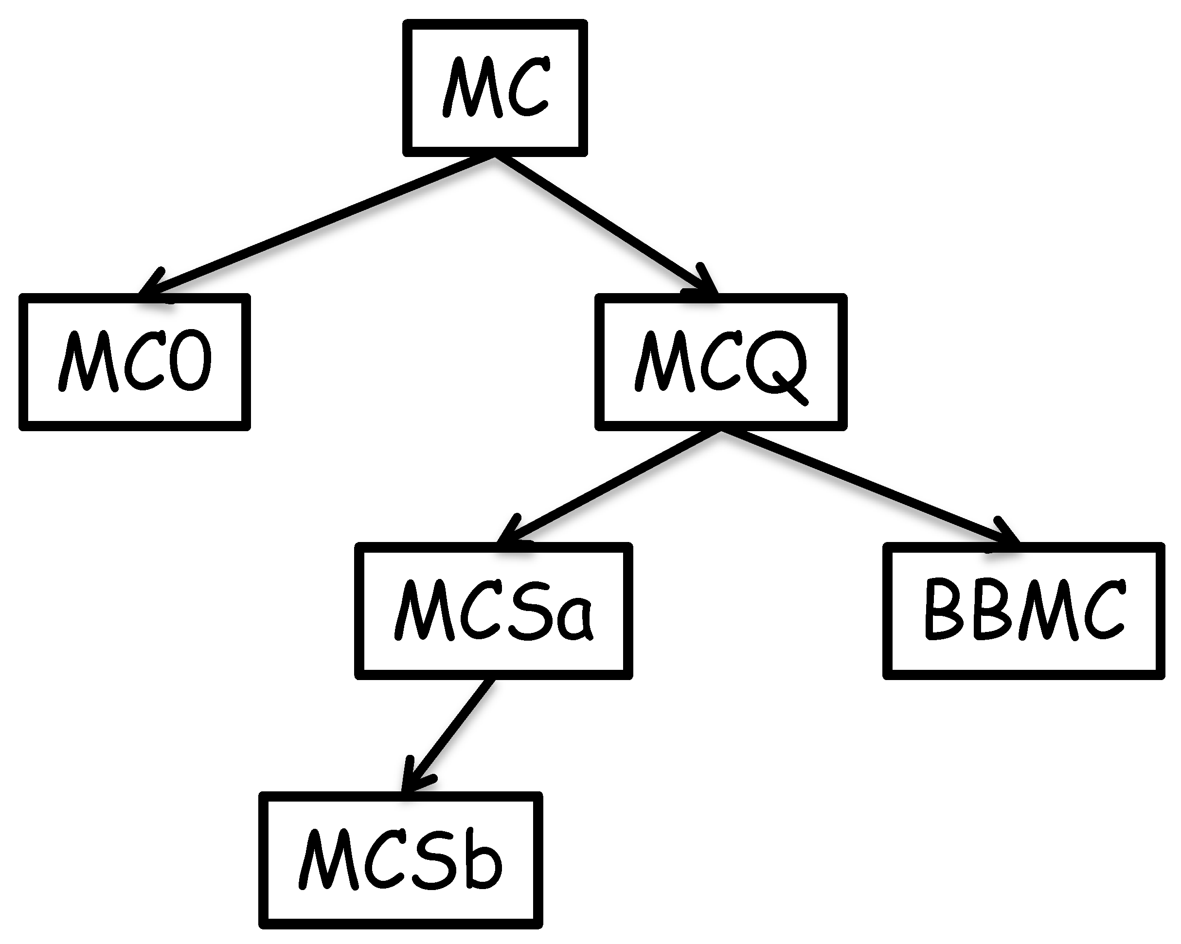
MC is essentially a straw man: It is elegant but too simple to be of any practical worth. Nevertheless, it has some interesting features. MCQ [12] is then presented as an extension to MC, our first algorithm that uses a tight integration of search algorithm, search order and upper bound cut off. Our implementation of MCQ allows three different vertex orderings to be used, and one of these corresponds to MCR [15]. The presentation of MCQ is somewhat laborious but this pays off when we present two variants of MCS [13] (MCSa and MCSb) as minor changes to MCQ. BBMC [11] is presented as an extension of MCQ, but is essentially MCSa with sets implemented using bit strings. Figure 1 shows the hierarchical structure for the algorithms presented. In the code presented, we endeavour to use the same procedure names as in the original publications.
Figure 1.
The hierarchy of algorithms.

2.1. MC
MC is similar to Algorithm 1 in [4]. Fahle’s Algorithm 1 uses two sets: C the growing clique (initially empty) and P the candidate set (initially all vertices in the graph). C is maximal when P is empty and if is a maximum it is saved, i.e., C becomes the champion. If is too small to unseat the champion search can be terminated. Otherwise the search iterates over the vertices in P in turn selecting a vertex v, creating a new growing clique where and a new candidate set as the set of vertices in P that are adjacent to v (i.e., ), and recursing. We will call this MC.
Listing 1. The basic clique solver.

2.1.1. MC in Java
Listing 1 can be compared with Algorithm 1 in [4]. The constructor, lines 14 to 22, takes three arguments: n the number of vertices in the graph, A the adjacency matrix where equals 1 if and only if vertex i is adjacent to vertex j, and where is the number of vertices adjacent to vertex i (and is the sum of ). The variables and are used as measures of search performance, is a bound on the run-time, is the size of the largest clique found so far, is used as a flag to customise the algorithm with respect to ordering of vertices (and is not used till we get to MCQ), and the array is the largest clique found such that is equal to 1 if and only if vertex i is in the largest clique found.
The method finds a largest clique or terminates when having exceeded the allocated . Two sets are produced: The candidate set P and the current clique C. Vertices from P may be selected and added to the growing clique C. Initially all vertices are added to P and C is empty (lines 27 to 29). The sets P and C are represented using Java’s ArrayList, a resizable-array implementation of the List interface. Adding an item is an operation but removing an arbitrary item is of cost. This might appear to be a damning indictment of this simple data structure, but as we will see, it is the cost we pay if we want to maintain order in P, and in many cases we can work around this to enjoy performance.
The search is performed in method . In line 34, a test is performed to determine if the CPU time limit has been exceeded, and if so search terminates. Otherwise we increment the number of nodes, i.e., a count of the size of the backtrack search tree explored. The method then iterates over the vertices in P (line 36), starting with the last vertex in P down to the first vertex in P. This form of iteration over the ArrayList, getting entries with a specific index, is necessary when entries are deleted (line 45) as part of that iteration. A vertex v is selected from P (line 38), added to C (line 39), and a new candidate set is then created (line 40) where is the set of vertices in P that are adjacent to vertex v (line 41). Consequently all vertices in are adjacent to all vertices in C and all pairs of vertices in C are adjacent (i.e., C is a clique). If is empty C is maximal and if it is the largest clique found it is saved (line 42). If is not empty then C is not maximal and search can proceed via a recursive call to (line 43). On returning from the recursive call v is removed from P and from C (lines 44 and 45).
There is one “trick” in and that is at line 37: If the combined size of the current clique and the candidate set cannot unseat the champion, this branch of the backtrack tree can be abandoned. This is the simplest upper bound cut-off and corresponds to line 3 from Algorithm 1 in [4]. The method saves off the current maximal clique and records its size.
2.1.2. Observations on MC
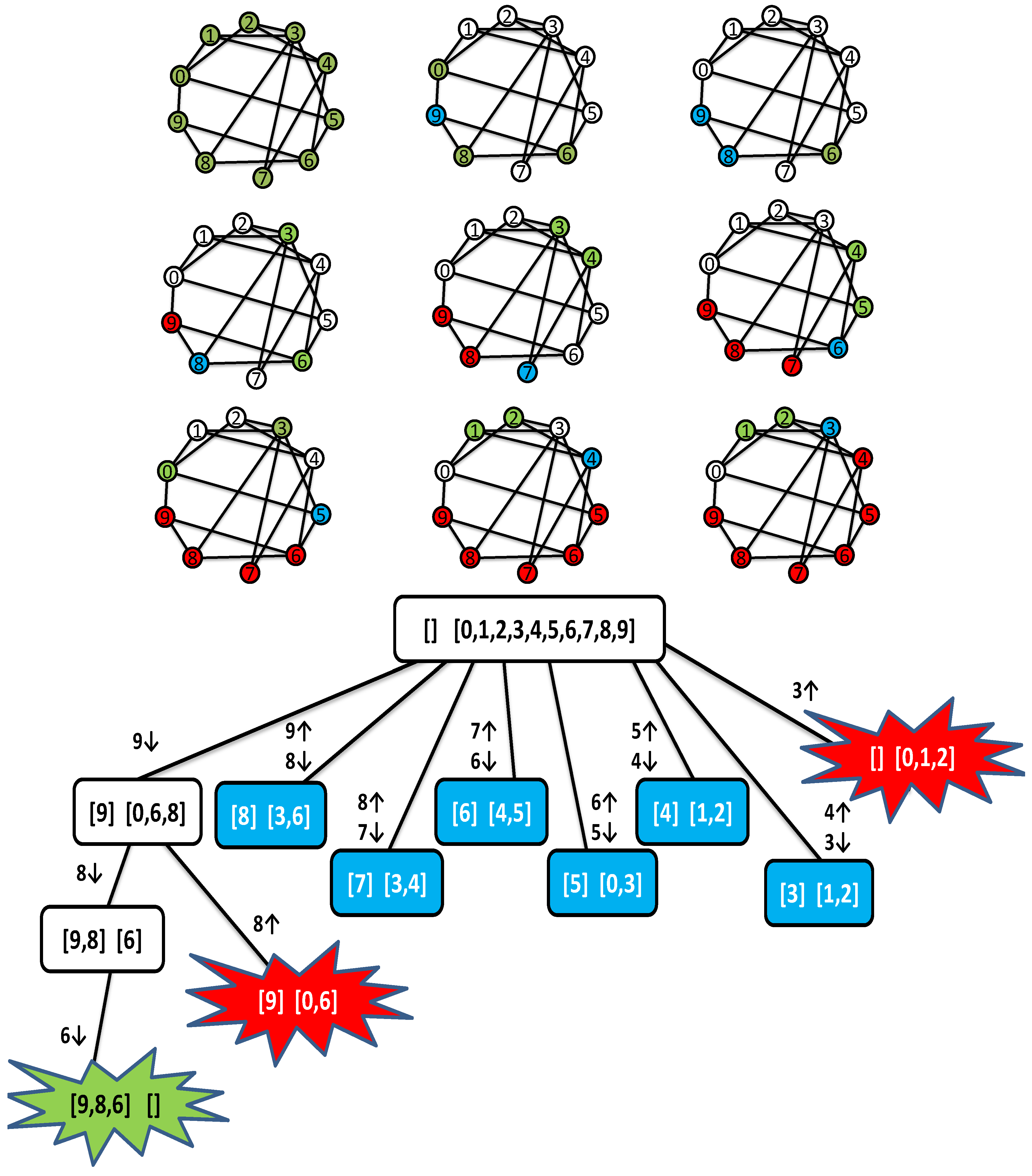
There are several points of interest. First, there is the search process itself. If we commented out lines 37 and changed line 41 to add to all vertices in P other than v, method would produce the power set of P and at each depth k in the backtrack tree we would have calls to . That is, produces a binomial backtrack search tree of size (see pages 6 and 7 of [17]). This can be compared to a bifurcating search process where on one side we take an element and make a recursive call, and on the other side reject it and make a recursive call, terminating when P is empty (i.e., generating a binary backtrack tree such as in [6,8,18]). This generates the power set on the leaf nodes of the backtrack tree and explores nodes. This is also but in practice is often twice as slow as the binomial search. In Figure 2 we see a binomial search produced by a simplification of MC, generating the power set of . Each node in the tree contains two sets: The set that will be added to the power set and the set that can be selected from at the next level. We see 16 nodes and at each depth k we have nodes. The corresponding tree for the bifurcating search (not shown) has 31 nodes with the power set appearing on the 16 leaf nodes at depth 4.
Figure 2.
A binomial search tree producing the power set of .

The second point of interest is the actual Java implementation. Java gives us an elegant construct for iterating over collections, the for-each loop, used in line 41 of Listing 1. This is rewritten in class MC0 (extending MC, overwriting the method) Listing 2 lines 15 to 18: One line of code is replaced with 4 lines. MC0 gets the element of P, calls it w (line 16 of Listing 2) and if it is adjacent to v it is added to (line 17 of Listing 2). In MC (line 41 of Listing 1) the for-each statement implicitly creates an iterator object and uses that for selecting elements. This typically results in a 10% reduction in runtime for MC0.
Our third point is how we create our sets. In MC0 line 14 the new candidate set is created with a capacity of i. Why do that when we can just create with no size and let Java work it out dynamically? And why size i?
Listing 2. Inelegant but 50% faster, MC0 extends MC.

In the loop of line 10 i counts down from the size of the candidate set, less one, to zero. Therefore at line 14 P is of size and we can set the maximum size of accordingly. If we do not set the size Java will give an initial size of 10 and when additions exceed this will be re-sized. By grabbing this space we avoid that. This results in yet another measurable reduction in run-time.
Our fourth point is how we remove elements from our sets. In MC we remove the current vertex v from C and P (lines 44 and 45) whereas in MC0 we remove the last element in C and P (lines 21 and 22). Clearly v will always be the last element in C and P. The code in MC results in a sequential scan to find and then delete the last element, i.e., , whereas in MC0 it is a simple task. This raises another question: P and C are really stacks so why not use a Java Stack? The Stack class is represented using an ArrayList and cannot be initialised with a size, but has a default initial size of 10. When the stack grows and exceeds its current capacity, the capacity is doubled and the contents are copied across. Experiments showed that using a Stack increased run time by a few percentage points.
Typically MC0 is 50% faster than MC. In many cases a 50% improvement in run time would be considered a significant gain, usually brought about by changes in the algorithm. Here, such a gain can be achieved by moderately careful coding. And this is our first lesson: When comparing published results, we need to be cautious as we may be comparing programmer ability as much as differences in algorithms.
The fifth point is that MC makes more recursive calls than it needs to. At line 37 is sufficient to proceed but at line 43 it is possible that is actually too small and will generate a failure at line 37 in the next recursive call. We should have a richer condition at line 43 but as we will soon see, the algorithms that follow do not need this.
The sixth point is a question of space: Why is the adjacency matrix an array of integers when we could have used booleans, surely that would have been more space efficient? In Java a boolean is represented as an integer with 1 being true, everything else false. Therefore there is no saving in space and only a minuscule saving in time (more code is generated to test if equals 1 than to test if a boolean is true). Furthermore, by representing the adjacency matrix as integers, we can sum a row to get the degree of a vertex.
Finally, Listing 1 shows exactly what is measured. Our run time starts at line 25, at the start of search. This will include the times to set up the data structures peculiar to an algorithm, and any reordering of vertices. It does not include the time to read in the problem or the time to write out a solution. There is also no doubt about what we mean by a node: A call to counts as one more node.
2.1.3. A Trace of MC
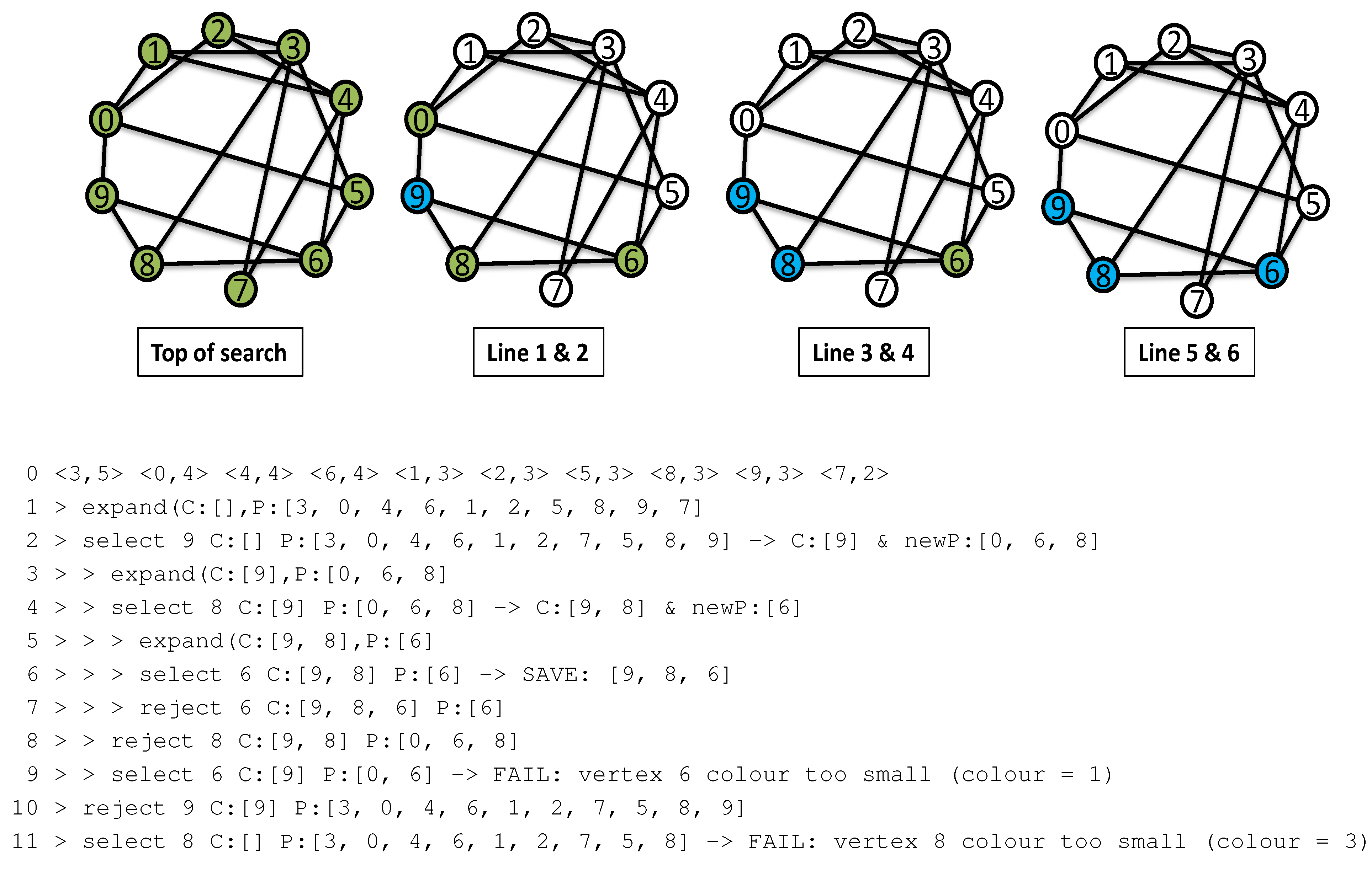
We now present two views of the MC search process over a simple problem. The problem is referred to as g10–50, and is a randomly generated graph with 10 vertices with edge probability 0.5. This is shown in Figure 3 and has at top a cartoon of the search process, to be read from left to right and top to bottom. Green coloured vertices are in P, blue vertices are those in C and red vertices are those removed from P and C in lines 44 and 45 of Listing 1. Also shown is the backtrack tree. The boxes correspond to calls to and contain C and P. On arcs we have numbers with a down arrow ↓ if that vertex is added to C and an up arrow ↑ if that vertex is removed from C and P, therefore C represent the path from the root to the current node. A clear white box is a call to that is an interior node of the backtrack tree leading to further recursive calls or the creation of a new champion. The green “shriek!” is a champion clique and a red “shriek!” is a failure because was too small to unseat the champion. The blue boxes correspond to calls to that fail first time on entering the loop at line 36 of Listing 1. By looking at the backtrack tree we get a feel for the nature of binomial search.
2.2. MCQ and MCR
We now present Tomita’s algorithm MCQ [12] as Listings 3–7. MCQ is at heart an extension of MC, performing a binomial search, with two significant advances. First, the graph induced by the candidate set is coloured using a greedy sequential colouring algorithm. This gives an upper bound on the size of the clique in P that can be added to C. Vertices in P are then selected in decreasing colour order, that is, P is ordered in non-decreasing colour order (highest colour last). And this is the second advance. Assume we select the entry in P and call it v. We then know that we can colour all the vertices in P corresponding to the 0th entry up to and including the entry using no more than the colour number of v. Consequently that sub-graph can contain a clique no bigger than the colour number of v, and if this is too small to unseat the largest clique, the search can be abandoned.
Figure 3.
Cartoon, trace and backtrack-tree for MC on graph g10–50.

2.2.1. MCQ in Java
MCQ extends MC, Listing 3 line 3, and has an additional instance variable (line 5) such that is an ArrayList of integers (line 15) and will contain all the vertices of colour and is used when sorting vertices by their colour (lines 45 to 64, Listing 4). At the top of search (method , lines 12 to 21, Listing 3) vertices are sorted (call to at line 19) into some order, and this is described later.
Method (line 23 to 43 Listing 3) corresponds to the method of the same name in Figure 2 of [12]. The array is local to the method and holds the colour of the vertex in P. The candidate set P is then sorted in non-decreasing colour order by the call to in line 28, and is then the colour of integer vertex . The search then begins in the loop at line 29. We first test to see if the combined size of the candidate set plus the colour of vertex v is sufficient to unseat the champion (line 30). If it is insufficient, the search terminates. Note that the loop starts at (line 29), the position of the last element in P, and counts down to zero. The element of P is selected and assigned to v. As in MC we create a new candidate set , the set of vertices (integers) in P that are adjacent to v (lines 33 to 37). We then test to see if C is maximal (line 38) and if it unseats the champion. If the new candidate set is not empty, we recurse (line 39). Regardless, v is removed from P and from C (lines 40 and 41).
Listing 3. MCQ (part 1), Tomita 2003.

Listing 4. MCQ (part 1 continued), Tomita 2003.

Listing 5. Vertex.

Listing 6. MCRComparator.

Listing 7. MCQ (part 2), Tomita 2003.

Method (Listing 4) can be compared to the method of the same name in Figure 3 of [12]. takes as arguments the current clique C, an ordered of integers corresponding to vertices to be coloured in that order, an of integers P that will correspond to the coloured vertices in non-decreasing colour order, and an array of integers such that if (v is the vertex in P) then the colour of v is . Lines 45 to 64 (Listing 4) differs from Tomita’s NUMBER-SORT method because we use the additional arguments and the growing clique C as this allows us to easily implement our next algorithm MCS (clique C is not used in until we get to MCSb, therefore we carry it for convenience only.)
Rather than assigning colours to vertices explicitly, places vertices into colour classes, i.e., if a vertex is not adjacent to any of the vertices in then that vertex can be placed into that class and given colour number ( so that colours range from 1 upwards). The vertices can then be sorted into colour order via a pigeonhole sort, where colour classes are the pigeonholes.
starts by clearing out the colour classes that might be used (line 48). In lines 49 to 55 vertices are selected from and placed into the first colour class in which there are no conflicts, i.e., a class in which the vertex is not adjacent to any other vertex in that class (lines 51 to 53, and method ). The variable records the number of colours used. Lines 56 to 63 is a pigeonhole sort, starting by clearing P and then iterating over the colour classes (loop start at line 58) and in each colour class adding those vertices into P (lines 59 to 63). The boolean method , lines 66 to 72, takes a vertex v and an ArrayList of vertices where vertices in are not pair-wise adjacent and have the same colour, i.e., the vertices are an independent set. If vertex v is adjacent to any vertex in , the method returns true (lines 67 to 70), otherwise false. Note that if vertex v needs to be added into a new colour class in , the size of that will be zero, and the for loop of lines 67 to 70 will not be performed and returns true. The complexity of is quadratic in the size of P.
Vertices need to be sorted at the top of search, line 19. To do this we use the class Vertex in Listing 5 and the comparator MCRComparator in Listing 6. If i is a vertex in P then the corresponding Vertex v has an integer equal to i. The Vertex also has attributes and . is the degree of the vertex and is the sum of the degrees of the vertices in the neighbourhood of vertex . Given an array V of class Vertex, this can be sorted using Java’s method in time, and is ordered by default using the method in class Vertex. Our method forces a strict ordering of V by non-increasing degree, tie-breaking on . This ensures reproducibility of results. If we allowed the to deliver 0 when two vertices have the same degree, then would break ties. If the sort method was unstable, i.e., it did not maintain the relative order of objects with equal keys [19], results may be unpredictable.
The class MCRComparator (Listing 6) allows us to sort vertices by non-increasing degree, tie breaking on the sum of the neighbourhood degree and then on , giving again a strict order. This is the MCR order given in [15], where MCQ uses the simple degree ordering and MCR is MCQ with tie-breaking on neighbourhood degree.
Vertices can also be sorted into a minimum-width order. Given an ordered set of vertices, the width of a vertex is the number of edges that lead from that vertex to previous vertices in the order, and the width of the ordering is the maximum width of its vertices. The minimum width order (mwo) was proposed by Freuder [20] and also by Matula and Beck [21] where it was called “smallest last”, and more recently in [16] as a degeneracy ordering. The method , lines 86 to 98 of Listing 7, sorts the array V of Vertex into an “mwo”. The vertices of V are copied into an ArrayList L (lines 87 and 89). The while loop starting at line 90 selects the vertex in L with smallest degree (lines 91 and 92) and calls it v. Vertex v is pushed onto the stack S and removed from L (line 93) and all vertices in L that are adjacent to v have their degree reduced (line 94). On termination of the while loop, vertices are popped off the stack and placed back into V, giving a minimum width (smallest last) ordering.
Method (Listing 7 lines 74 to 84) is then called once, at the top of search. The array of Vertex V is created for sorting in lines 75 and 76, and the sum of the neighbourhood degrees is computed in lines 77 to 79. is then sorted in one of three orders: in non-increasing degree order, in minimum width order, in non-increasing degree tie-breaking on sum of neighbourhood degree. MCQ then uses the ordered candidate set P for colouring, initially in one of the initial orders, thereafter in the order resulting from and that is non-decreasing colour order. In [12] it is claimed that this is an improving order (however, no evidence was presented for this claim). In [15] Tomita proposes a new algorithm, MCR, where MCR is MCQ with a different initial ordering of vertices, i.e., MCQ with .
2.2.2. A Trace of MCQ
Figure 4 shows a cartoon and trace of MCQ over graph g10-50. Print statements were placed immediately after the call to (Listing 3 line 24), after the selection of a vertex v (line 31) and just before v is rejected from P and C (line 40). Each picture in the cartoon gives the corresponding line numbers in the trace immediately below. Line 0 of the trace is a print-out of the ordered array V just after line 83 in method in Listing 7. This shows for each vertex the pair : the first call to has , i.e., non-decreasing degree order. MCQ makes 3 calls to whereas MC makes 9 calls, and the MCQ colour bound cut-off in line 30 of Listing 3 is satisfied twice (Figure 4 lines 9 and 11).
Figure 4.
Trace of MCQ1 on graph g10–50.

2.2.3. Observations on MCQ
We noted above that MC can make recursive calls that immediately fail. Can this happen in MCQ? Looking at lines 39 of Listing 3, must be greater than . Since the colour of the vertex selected was sufficient to satisfy the condition of line 30, it must be that integer vertex v (line 31) is adjacent to at least vertices in P and thus in , therefore the next recursive call will not immediately fail. Consequently each call to corresponds to an internal node in the backtrack tree.
We also see again exactly what is measured as CPU time: It includes the creation of our data structures, the reordering of vertices at the top of search and all recursive calls to (lines 12 to 20).
Why is an ArrayList rather than an ArrayList<ArrayList<Integer>>? That would have done away with the explicit cast in line 60. When using an ArrayList<ArrayList<Integer>> Java generates an implicit cast, so nothing is gained—it is merely syntactic sugar.
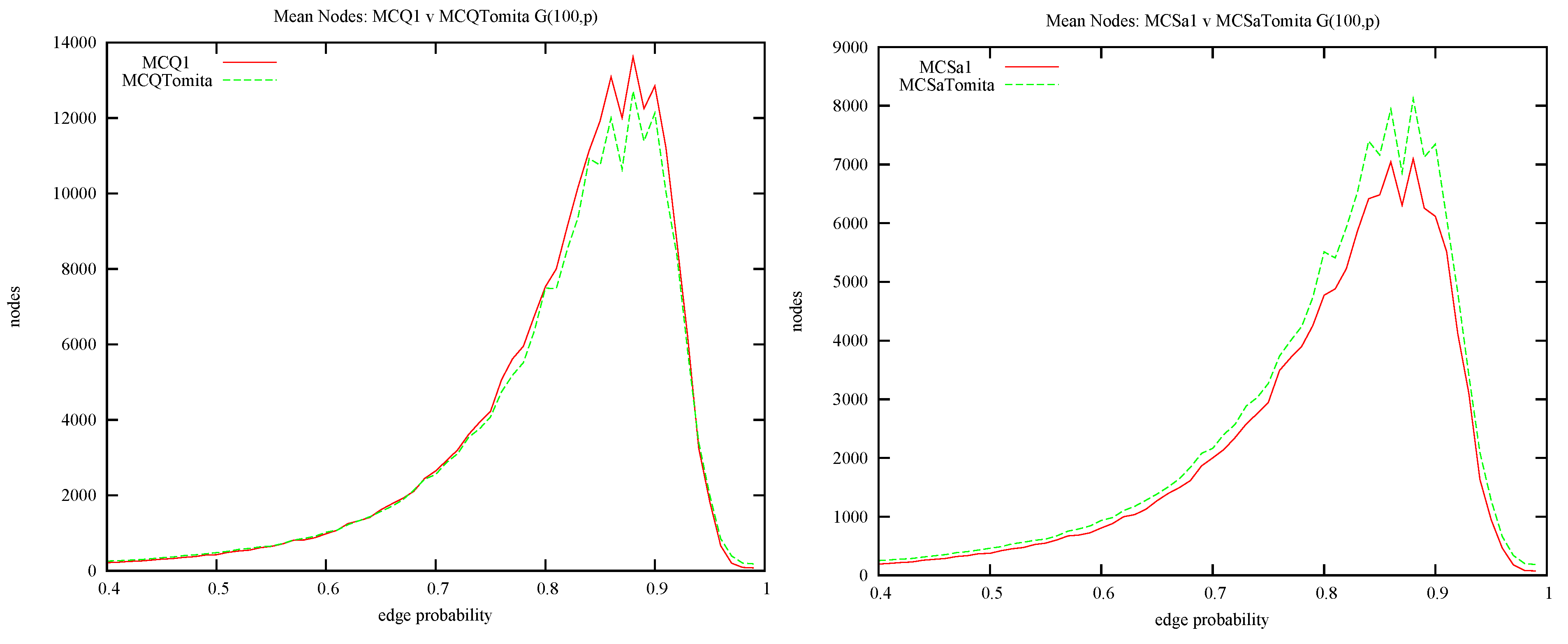
Tomita’s presentation of MCQ [12] differs from Listing 3 in that it initially colours the sorted vertices prior to calling and thereafter colour-sorts the new candidate set immediately before making a recursive call to . Appendix 1 explains this in detail and investigates the effect on performance.
2.3. MCS
In [13] MCS is presented as two modifications to MCQ. The first modification is to use “... an adjunct ordered set of vertices for approximate coloring”. This is an ordered list of vertices to be used in the sequential colouring, and was called . This order is static, set at the top of search. Therefore, rather than using the order in the candidate set P for colouring the vertices in P, the vertices in P are coloured in the order of vertices in .
The second modification is to use a repair mechanism when colouring vertices (this is called a Re-NUMBER in Figure 1 of [13]). When colouring vertices, an attempt is made to reduce the colours used by performing exchanges between vertices in different colour classes. In [13] a recolouring of a vertex v occurs when a new colour class is about to be opened for v and that colour class exceeds the search bound, i.e., if the number of colours can be reduced, this could result in search being cut off. In the context of colouring, I will say that vertex u and v conflict if they are adjacent, and that v conflicts with a colour class C if there exists a vertex that is in conflict with v. Assume vertex v is in colour class . If there exists a lower colour class () and v conflicts with only a single vertex and there also exists a colour class , where , and w does not conflict with any vertex in , then we can place v in and w in , freeing up colour class . This is given in Figure 1 of [13] and the procedure is named Re-NUMBER.
Figure 5 illustrates this procedure. The boxes correspond to colour classes i, j and k where . The circles correspond to vertices in that colour class and the red arrowed lines as conflicts between pairs of vertices. Vertex v has just been added to colour class k, v conflicts only with w in colour class i, and w has no conflicts in colour class j. We can then move w up to colour class j and v down to colour class i.
Figure 5.
A repair scenario with colour classes i, j and k.

Experiments were then presented in [13] comparing MCR against MCS in which MCS is always the champion. But it is not clear where the advantage of MCS comes from: Does it come from the static colour order (the “adjunct ordered set”) or does it come from the colour repair mechanism?
I now present two versions of MCS. The first, which I call MCSa, uses the static colouring order. The second, MCSb, uses the static colouring ordering and the colour repair mechanism (so MCSb is Tomita’s MCS). Consequently, we will be able to determine where the improvement in MCS comes from: Static colour ordering or colour repair.
2.3.1. MCSa in Java
In Listing 8 we present MCSa as an extension to MCQ. Method creates an explicit colour ordering and the method is called with this in line 18 (compare this to line 20 of MCQ). Method now takes three arguments: The growing clique C, the candidate set P and the colouring order . In line 26 is called using (compare with line 28 in MCQ) and lines 27 to 45 are essentially the same as lines 29 to 42 in MCQ with the exception that must also be copied and updated (lines 32, 36 and 37) prior to the recursive call to (line 40) and then down-dated after the recursive call (line 43). Therefore, MCSa is a simple extension of MCQ and, like MCQ, has three styles of ordering.
2.3.2. MCSb in Java
In Listing 9 we present MCSb as an extension to MCSa: The difference between MCSb and MCSa is in , with the addition of lines 10 and 20. At line 10 we compute as the minimum number of colour classes required to match the search bound. At line 20, if we have exceeded the number of colour classes required to exceed the search bound and a new colour class k has been opened for vertex v and we can repair the colouring such that one less colour class is used, we can decrement the number of colours used. This repair is done in the boolean method of lines 43 to 57. The method returns true if vertex v in colour class k can be recoloured into a lower colour class, false otherwise, and can be compared to Tomita’s Re-NUMBER procedure. We search for a colour class i, where , in which there exists only one vertex in conflict with v and we call this w (line 45). The method , lines 32 to 41, searches for such a vertex. It takes as arguments a vertex v and a colour class . If v is adjacent to only one vertex in the index of that vertex is returned (line 40), where , otherwise a negative number is returned (line 39). The method then proceeds at line 46 if a single conflicting vertex w was found, searching for a colour class j above i (for loop of line 47) in which there are no conflicts with w. If that was found (line 48), vertex v is removed from colour class k, w is removed from colour class i, v is added to colour class i and w to colour class j (lines 49 to 52), and delivers (line 53). Otherwise, no repair occurred (line 56).
Listing 8. MCSa, Tomita 2010.

Listing 9. MCSb, Tomita 2010.

2.3.3. Observations on MCS
Tomita did not investigate where MCS’s improvement comes from and neither did [2], coding up MCS in Python in one piece. However San Segundo did [10], incrementally adding colour repair to BBMC. We can also tune MCS. In MCSb we repair colourings when we open a new colour class that exceeds the search bound. We could instead repair unconditionally every time we open a new colour class, attempting to maintain a compact colouring. We do not investigate this here.
2.4. BBMC
San Segundo’s BB-MaxClique algorithm [11] (BBMC) is similar to the earlier algorithms in that vertices are selected from the candidate set to add to the current clique in non-increasing colour order, with a colour cut-off within a binomial search. BBMC is at heart a bit-set encoding of MCSa with the following features.
- The “BB” in “BB-MaxClique” is for “Bit Board”. Sets are represented using bit strings.
- BBMC colours the candidate set using a static sequential ordering, the ordering set at the top of search, the same as MCSa.
- BBMC represents the neighbourhood of a vertex and its inverse neighbourhood as bit strings, rather than using a row of an adjacency matrix and its complement.
2.4.1. BBMC in Java
We implement sets using Java’s BitSet class (a vector of bits with associated methods) and from now on we refer to P as the candidate BitSet and an ordered array of integers U as the ordered candidate set. In Listing 10, lines 5 to 7, we have an array of BitSet N for representing neighbourhoods, as the inverse neighbourhoods (the complement of N) and V an array of Vertex. is then a BitSet representing the neigbourhood of the vertex in the array V, and as its complement. The array V is used at the top of search for renaming vertices (and we discuss this later).
The method (lines 16 to 30) creates the candidate BitSet P, current clique (as a BitSet) C, and Vertex array V. The method renames the vertices and will be discussed later. The method corresponds to the procedure in Figure 3 of [11] and can be compared to the method in Listing 8. In a BitSet we use rather than (line 35, 40 and 44). The integer array U (same name as in [11]) is essentially the colour ordered candidate set such that if then corresponds to the colour given to v and . The method call of line 38 colours the vertices and delivers those colours in the array and the sorted candidate set in U. The for loop, lines 39 to 47 (again, counting down from to zero), first tests to see if the colour cut-off occurs (line 40) and if it does the method returns.
Listing 10. San Segundo’s BB-MaxClique in Java (part 1).

Otherwise a new candidate BitSet is created, on line 41, as a clone of P. The current vertex v is then selected (line 42) and in line 43 v is added to the growing clique C and becomes the BitSet corresponding to the vertices in the candidate BitSet that are in the neighbourhood of v. The operation (line 43) is equivalent to the for loop in lines 34 to 37 of Listing 3 of MCQ. If the current clique is both maximal and a maximum, it is saved via BBMC’s specialised save method (described later), otherwise if C is not maximal (i.e., is not empty) a recursive call is made to . Regardless, v is removed from the current candidate BitSet and the current clique (line 46) and the for loop continues.
Method (Listing 11) corresponds to the procedure of the same name in Figure 2 of [11] but differs in that it does not explicitly represent colour classes and therefore does not require a pigeonhole sort as in San Segundo’s description. Our method takes the candidate BitSet P (see line 38), ordered candidate set U and array of as parameters. Due to the nature of Java’s BitSet the operation is not functional but actually modifies bits, consequently cloning is required (line 51 Listing 11) and we take a copy of P. In line 52 records the current colour class, initially zero, and i is used as a counter for adding coloured vertices into the array U. The while loop, lines 54 to 64, builds up colour classes whilst consuming vertices in . The BitSet Q (line 56) is the candidate BitSet as we are about to start a new colour class. The while loop of lines 57 to 64 builds a colour class: The first vertex in Q is selected (line 58) and is removed from the candidate BitSet (line 59) and BitSet Q (line 60), Q then becomes the set of vertices that are in the current candidate BitSet (Q) and in the inverse neighborhood of v (line 61), i.e., Q becomes the BitSet of vertices that can join the same colour class with v. We then add v to the ordered candidate set U (line 62), record its colour and increment our counter (line 63). When Q is exhausted (line 57) the outer while loop (line 54) starts a new colour class (lines 55 to 64).
Listing 11. San Segundo’s BB-MaxClique in Java (part 1 continued).

Listing 12 shows how the candidate BitSet is renamed/reordered. In fact it is not the candidate BitSet that is reordered, rather it is the description of the neighbourhood N and its inverse that is reordered. Again, as in MCQ and MCSa, a Veretx array is created (lines 69 to 73) and is sorted into one of three possible orders (lines 74 to 76). Once sorted, a bit in position i of the candidate BitSet P corresponds to the integer vertex . The neighbourhood and its inverse are then reordered in the loop of lines 77 to 83. For all pairs , we select the corresponding vertices u and v from V (lines 79 and 80) and if they are adjacent then the bit of is set true, otherwise false (line 81). Similarly, the inverse neighbourhood is updated in line 82. The loop could be made twice as fast by exploiting symmetries in the adjacency matrix A. In any event, this method is called once at the top of search and is generally an insignificant contribution to run time.
Listing 12. San Segundo’s BB-MaxClique in Java (part 2).

BBMC requires its own method (lines 86 to 90 of Listing 12) due to C being a BitSet. Again the solution is saved into the integer array and again we need to use the Vertex array V to map bits to vertices. This is done in line 88: If the bit of C is true then integer vertex is in the solution. This explains why V is global to the class.
2.4.2. Observations on BBMC
In our Java implementation, we might expect a speedup if we did away with the in-built BitSet and did our own bit-string manipulations explicitly. It is also worth noting that in [10] comparisons are made with Tomita’s results in [13] by rescaling tabulated results, i.e., Tomita’s code was not actually run, but this is not unusual.
2.5. Summary of MCQ, MCR, MCS and BBMC
Putting aside the chronology [11,12,13,15], MCSa is the most general algorithm presented here. BBMC is in essence MCSa with a BitSet encoding of sets. MCQ is MCSa except that we do away with the static colour ordering and allow MCQ to colour and sort the candidate set using the candidate set, somewhat in the manner of Uroborus the serpent that eats itself. And MCSb is MCSa with an additional colour repair step.
3. Exact Algorithms for Maximum Clique: A Brief History
We now present a brief history of complete algorithms for the maximum clique problems, starting from 1990. The algorithms are presented in chronological order.
1990: In 1990 [3] Carraghan and Pardalos present a branch and bound algorithm. Vertices are ordered in non-decreasing degree order at each depth in the binomial search with a cut-off based on the size of the largest clique found so far. Their algorithm is presented in Fortran 77 along with code to generate random graphs; consequently, their empirical results are entirely reproducible. Their algorithm is similar to MC (Listing 1) but sorts the candidate set P using current degree in each call to .
1992: In [8] Pardalos and Rodgers present a zero-one encoding of the problem where a vertex v is represented by a variable that takes the value 1 if search decides that v is in the clique and 0 if it is rejected. Pruning takes place via the constraint (Rule 4). In addition, a candidate vertex adjacent to all vertices in the current clique is forced into the clique (Rule 5) and a vertices of degree too low to contribute to the growing clique is rejected (Rule 7). The branch and bound search selects variables dynamically based on current degree in the candidate set: A non-greedy selection chooses a vertex of lowest degree and greedy selects highest degree. The computational results showed that greedy was good for (easy) sparse graphs and non-greedy was good for (hard) dense graphs.
1994: In [22] Pardalos and Xue reviewed algorithms for the enumeration problem (counting maximal cliques) and exact algorithms for the maximum clique problem. Although dated, it continues to be an excellent review.
1997: In [14] graph colouring and fractional colouring is used to bound search. Comparing again to MC (Listing 1) the candidate set is coloured greedily, and if the size of the current clique plus the number of colours used is less than or equal to the size of the largest clique found so far, that branch of search is cut off. In [14] vertices are selected in non-increasing degree order, the opposite of that proposed by [8]. We can get a similar effect to [14] in MC if we allow free selection of vertices, colour between lines 42 and 43 and make the recursive call to in line 43 conditional on the colour bound.
2002: Patric R. J. Östergård proposed an algorithm that has a dynamic programming flavour [7]. The search process starts by finding the largest clique containing vertices drawn from the set and records it size in . Search then proceeds to find the largest clique in the set using the value in as a bound. The vertices are ordered at the top of search in colour order, i.e., the vertices are coloured greedily and then ordered in non-decreasing colour order, similar to that in Listing 4. Östergård’s algorithm is available as Cliquer [7]. In the same year, Torsten Fahle [4] presented a simple algorithm (Algorithm 1) that is essentially MC but with a free selection of vertices rather than the fixed iteration in line 36 of Listing 1 and dynamic maintenance of vertex degree in the candidate set. This is then enhanced (Algorithm 2) with forced accept and forced reject steps similar to Rules 4, 5 and 7 of [8] and the algorithm is named DF (Domain Filtering). DF is then enhanced to incorporate a colouring bound, similar to that in Wood [14].
2003: Jean-Charles Régin proposed a constraint programming model for the maximum clique problem [9]. His model uses a matching in a duplicated graph to deliver a bound within search, a Not Set as used in the Bron Kerbosch enumeration Algorithm 457 [23] and vertex selection using the pivoting strategy similar to that in [16,23,24,25]. That same year Tomita reported MCQ [12].
2004: Faisal N. Abu-Khzam et al. [26] presented a number of kernelization steps to reduce a graph before and during search in the vertex cover problem, where a minimum vertex cover of the complement graph is a maximal clique in the original graph. Some of the kernelization steps are similar to the pruning rules in [4,8] although Crown Reduction appears to be novel and effective.
2007: Tomita proposed MCR [15] and in the same year Janez Konc and Dus̆anka Janez̆ic̆ proposed the MaxCliqueDyn algorithm [5]. The algorithm is essentially MCQ [12] with dynamic reordering of vertices in the candidate set, using current degree, prior to colouring. This reordering is expensive and takes place high up in the backtrack tree and is controlled by a parameter . Varying this parameter influences the cost of the search process and must be tuned on an instance-by-instance basis.
2010: Pablo San Segundo and Cristóbal Tapia presented an early version of BBMC (BB-MCP) [27] and Tomita presented MCS [13]. In the same year Li and Quan proposed new max-SAT encodings for maximum clique [6,18].
2011: Pablo San Segundo proposed BBMC [11] and BBMCR [10], where BBMCR includes a colour repair step. In [10] it is noted that in [13] “... the concrete contribution of recolouring is unfortunately not made explicit.” San Segundo’s colour repair, differs from that in Listing 9 in that a single swap can occur after a double swap (as in lines 49 to 52 of Listing 9). This cannot occur in Listing 9 because (line 43) is called only when a new colour class k is opened for vertex v (line 20); consequently v must have been adjacent to at least one vertex in each colour class less than k and therefore (line 34) cannot be equal to zero at line 40.
2012: Renato Carmo and Alexandre P. Züge [2] reported an empirical study of 8 algorithms including those from [3] and [4] along with MCQ, MCR, MCS and MaxCliqueDyn. The claim is made that the Bron Kerbosch algorithm provides a unified framework for all the algorithms studied, although a Not Set is not used. Neither do they use pivoting as described in [16,23,24,25]. All algorithms are coded in Python, therefore the study is objective (the authors include none of their own algorithms) and fair (all algorithms are coded by the authors and run in the same environment). BBMC is not include in the study, MCS is not broken into its constituent parts (MCSa and MCSb), and the study uses only the DIMACS benchmarks.
4. The Computational Study
The computational study attempts to answer the following questions.
- Where does the improvement in MCS come from? By comparing MCQ with MCSa we can measure the contribution due to static colouring, and by comparing MCSa with MCSb we can measure the contribution due to colour repair.
- How much benefit can be obtained from the BitSet encoding? We compare MCSa with BBMC over a variety of problems.
- We have three possible initial orderings (styles). Is any one of them better than the others and is this algorithm independent?
- Most papers use only random problems and the DIMACS benchmarks. What other problems might we use in our investigation?
- Is it safe to recalibrate published results?
Throughout our study we use a reference machine (named Cyprus), a machine with two Intel E5620 2.4 GHz quad-core processors with 48 GB memory, running Linux CentOS 5.3 and Java version 1.6.0_07.
4.1. MCQ vs. MCS: Static Ordering and Colour Repair
Is MCS faster than MCQ, and if so, why? MCSa is MCQ with a static colour ordering set at the top of search, and MCSb is MCSa with the colour repair mechanism. By comparing these algorithms, we can determine if indeed MCSb is faster than MCQ and where that gain comes from—the static colouring order or the colour repair. We start our investigation with Erdós–Rënyi random graphs where n is the number of vertices and each edge is included in the graph with probability p independent from every other edge.
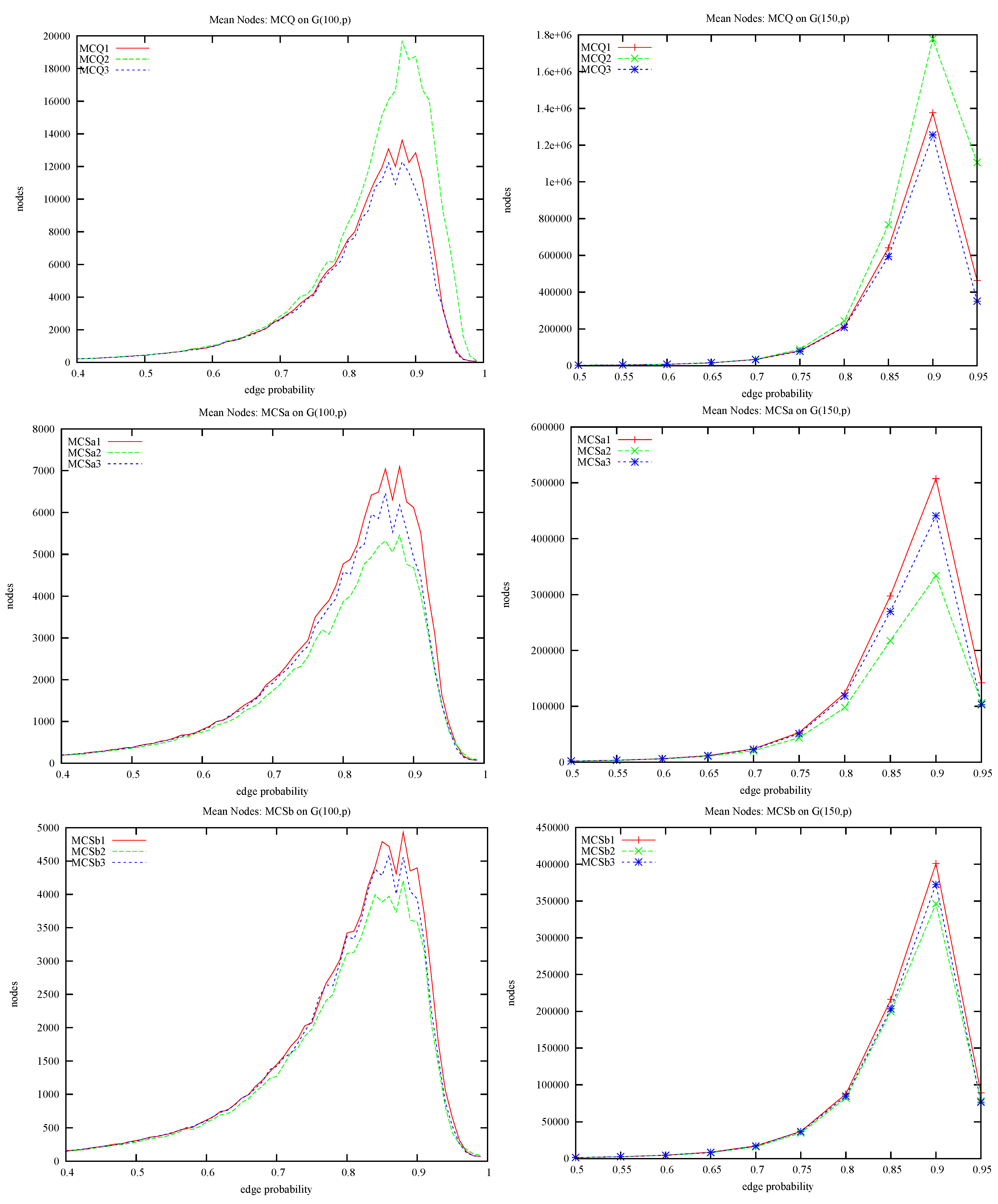
The first experiments are on random , first with , , p varying in steps of 0.01, sample size of 100, then with , , p varying in steps of 0.05, sample size of 100, and , , p varying in steps of 0.05, sample size of 100. Unless otherwise stated, all experiments are carried out on our reference machine. The algorithms MCQ, MCSa and MCSb all use (i.e., MCQ1, MCSa1, MCSb1). Figure 6 shows on the left the average number of nodes against the edge probability and on the right the average run time in milliseconds against the edge probability, for MCQ1, MCSa1 and MCSb1. The top row has , middle row and bottom row . For MCQ1 the sample size at was reduced to 28, i.e., the MCQ1-200 job was terminated after 60 hours. As we apply the modifications to MCQ, we see a reduction in nodes with MCSb1 exploring less states than MCSa1 and MCSa1 less than MCQ1. However, on the right we see that reduction in search space does not always result in reduction in run time. MCSb1 is always slower than MCSa1, i.e., the colour repair is too expensive and when MCSb1 is often more expensive to run than MCQ! Therefore, it appears that MCS gets its advantage just from the static colour ordering and that the colour repair slows it down.
Figure 6.
, sample size 100. MCQ vs. MCS, where is the win? (left) Search effort in nodes visited (i.e., decisions made by the search process); (right) run time in milliseconds.
Figure 6.
, sample size 100. MCQ vs. MCS, where is the win? (left) Search effort in nodes visited (i.e., decisions made by the search process); (right) run time in milliseconds.


| instance | MCQ1 | MCSa1 | MCSb1 | ||||||
|---|---|---|---|---|---|---|---|---|---|
| brock200-1 | 868,213 | 7 | (21) | 524,723 | 4 | (21) | 245,146 | 3 | (21) |
| brock400-1 | 342,473,950 | 4,471 | (27) | 198,359,829 | 2,888 | (27) | 142,253,319 | 2,551 | (27) |
| brock400-2 | 224,839,070 | 2,923 | (29) | 145,597,994 | 2,089 | (29) | 61,327,056 | 1,199 | (29) |
| brock400-3 | 194,403,055 | 2,322 | (31) | 120,230,513 | 1,616 | (31) | 70,263,846 | 1,234 | (31) |
| brock400-4 | 82,056,086 | 1,117 | (33) | 54,440,888 | 802 | (33) | 68,252,352 | 1,209 | (33) |
| brock800-1 | 1,247,519,247 | — | (23) | 1,055,945,239 | — | (23) | 911,465,283 | — | (21) |
| brock800-2 | 1,387,973,191 | — | (21) | 1,171,057,646 | — | (24) | 914,638,570 | — | (21) |
| brock800-3 | 1,332,309,827 | — | (21) | 1,159,165,900 | — | (21) | 914,235,793 | — | (21) |
| brock800-4 | 804,901,115 | — | (26) | 640,444,536 | 12,568 | (26) | 659,145,642 | 13,924 | (26) |
| hamming10-4 | 636,203,658 | — | (40) | 950,939,457 | — | (37) | 858,347,653 | — | (37) |
| johnson32-2-4 | 10,447,210,976 | — | (16) | 8,269,639,389 | — | (16) | 7,345,343,221 | — | (16) |
| keller5 | 603,233,453 | — | (27) | 596,150,386 | — | (27) | 523,346,613 | — | (27) |
| keller6 | 285,704,599 | — | (48) | 226,330,037 | — | (52) | 240,958,450 | — | (54) |
| MANN-a27 | 38,019 | 9 | (126) | 38,019 | 6 | (126) | 38,597 | 8 | (126) |
| MANN-a45 | 2,851,572 | 4,989 | (345) | 2,851,572 | 3,766 | (345) | 2,545,131 | 4,118 | (345) |
| MANN-a81 | 550,869 | — | (1100) | 631,141 | — | (1100) | 551,612 | — | (1100) |
| p-hat1000-1 | 237,437 | 2 | (10) | 176,576 | 2 | (10) | 151,033 | 2 | (10) |
| p-hat1000-2 | 466,616,845 | — | (45) | 34,473,978 | 1,401 | (46) | 166,655,543 | 7,565 | (46) |
| p-hat1000-3 | 440,569,803 | — | (52) | 345,925,712 | — | (55) | 298,537,771 | — | (56) |
| p-hat1500-1 | 1,642,981 | 16 | (12) | 1,184,526 | 14 | (12) | 990,246 | 14 | (12) |
| p-hat1500-2 | 414,514,960 | — | (52) | 231,498,292 | — | (60) | 259,771,137 | — | (57) |
| p-hat1500-3 | 570,637,417 | — | (56) | 220,823,126 | — | (69) | 176,987,047 | — | (69) |
| p-hat300-3 | 3,829,005 | 74 | (36) | 624,947 | 13 | (36) | 713,107 | 21 | (36) |
| p-hat500-2 | 1,022,190 | 23 | (36) | 114,009 | 3 | (36) | 137,568 | 5 | (36) |
| p-hat500-3 | 515,071,375 | — | (47) | 39,260,458 | 1,381 | (50) | 104,684,054 | 4,945 | (50) |
| p-hat700-2 | 18,968,155 | 508 | (44) | 750,903 | 27 | (44) | 149,0522 | 74 | (44) |
| p-hat700-3 | 570,423,439 | — | (48) | 255,745,746 | — | (62) | 243,836,191 | — | (62) |
| san1000 | 302,895 | 20 | (15) | 150,725 | 10 | (15) | 53,215 | 3 | (15) |
| san200-0.9-2 | 1,149,564 | 20 | (60) | 229,567 | 5 | (60) | 62,776 | 1 | (60) |
| san200-0.9-3 | 8,260,345 | 154 | (44) | 6,815,145 | 111 | (44) | 1,218,317 | 32 | (44) |
| san400-0.7-1 | 55,010 | 1 | (40) | 119,356 | 2 | (40) | 134,772 | 3 | (40) |
| san400-0.7-2 | 606,159 | 14 | (30) | 889,125 | 19 | (30) | 754,146 | 16 | (30) |
| san400-0.7-3 | 582,646 | 11 | (22) | 521,410 | 10 | (22) | 215,785 | 5 | (22) |
| san400-0.9-1 | 523,531,417 | — | (56) | 4,536,723 | 422 | (100) | 582,445 | 54 | (100) |
| sanr200-0.7 | 206,262 | 1 | (18) | 152,882 | 1 | (18) | 100,977 | 1 | (18) |
| sanr200-0.9 | 44,472,276 | 892 | (42) | 14,921,850 | 283 | (42) | 9,730,778 | 245 | (42) |
| sanr400-0.5 | 380,151 | 2 | (13) | 320,110 | 2 | (13) | 190,706 | 2 | (13) |
| sanr400-0.7 | 101,213,527 | 979 | (21) | 64,412,015 | 711 | (21) | 46,125,168 | 650 | (21) |
We also see a region where problems are hard for all our algorithms, at and , both in terms of nodes and run time, and in [10] it is suggested that this behaviour is a “... phase transition to triviality ...”. However at there is a different picture. We see a hard region in terms of nodes but an ever-increasing run time. That is, even though nodes are falling, CPU time is climbing. This agrees with the tabulated results in [11] (Tables 4 and 5 on page 580) for BB-MaxClique. It is a conjecture that run time increases because the cost of each node (call to expand) incurs more cost in the colouring of the relatively larger candidate set. In going from to , the maximum clique size increased on average from 41 to 62, a 50% increase, and for MCSa1 the average number of nodes fell by 20% (30% for MCSb1). The search space has fallen and the clique size has increased, which increases the cost of colouring and results in an overall increase in run time. Therefore it does not appear to be a phase transition in the sense of [28,29,30], i.e., a feature of the problem that is algorithm independent.
We now report on the 66 DIMACS instances [31] in Table 1. For each algorithm, we have 3 entries: The number of nodes, CPU time in seconds, and in brackets the size of the largest clique found. Each algorithm was allowed 14,400 CPU seconds and if that was exceeded we have a table entry of “—”. The best CPU time in a row is in bold font, and when CPU time limit is exceeded, the largest maximum clique size is emboldened. Easy instances are not tabulated, i.e., those that took less than a second. Overall, we see that MCQ1 is rarely the best choice with MCSa1 or MCSb1 performing better. There are 11 problems where MCSb1 beats MCSa1 and 9 problems where MCSa1 beats MCSb1. Therefore, the DIMACS benchmarks do not significantly separate the behaviour of these two algorithms.
These results conflict somewhat with those in [10]. There it is claimed that colour repair, when added to BBMC, results in a performance gain in dense graphs (). Results are presented for a subset of the DIMACS instances with some of the difficult instances absent (brock800-*, hamming10-4, keller5, keller6, johnson32-2-4, MANN-a81, p-hat1000-3, p-hat1500-2, p-hat1500-3) and for random graphs with a sample size of 10.
4.2. BBMC vs. MCSa: A Change of Representation
What advantage is to be obtained from the change of representation between MCSa and BBMC, i.e., representing sets as in MCSa and as a BitSet in BBMC? MCSa and BBMC are at heart the same algorithm. They both produce the same colourings, order the candidate set in the same way and explore the same backtrack tree.
Figure 7.
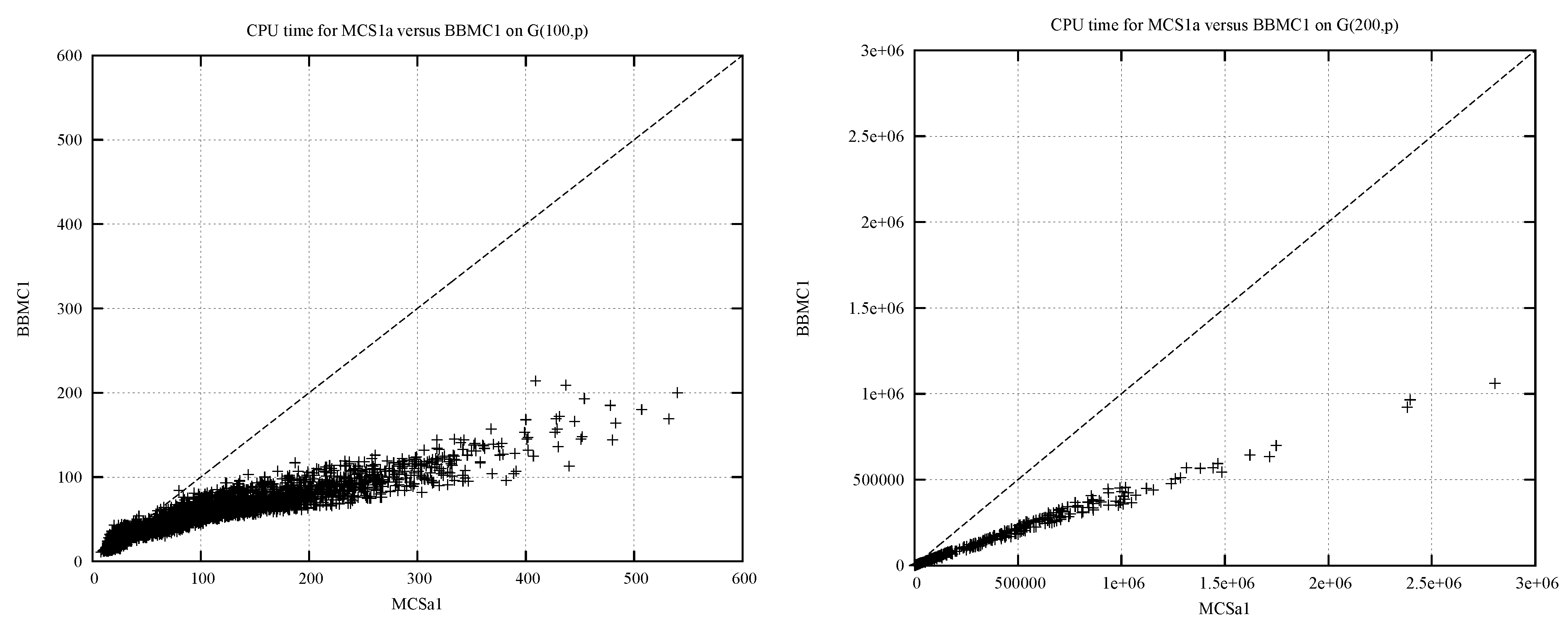
Run time of MCSa1 against BBMC1, on the left and on the right .

Figure 7 shows on the left the run time of MCSa1 (x-axis) against the run time of BBMC1 (y-axis) in milliseconds on each of the random instances and on the right for . The dotted line is the reference . If points are below the line then BBMC1 is faster than MCSa1. BBMC1 is typically twice as fast as MCSa1.
In Table 2 we tabulate Goldilocks instances from the DIMACS benchmark suite: We remove the instances that are too easy (take less than a second) and those that are too hard (take more than 4 h), leaving those that are “just right” for both algorithms. Under each algorithm, we have: Nodes visited (and this is the same for both algorithms), run time (in seconds), and in brackets the size of the maximum clique. The column on the far right is the ratio of MCSa1’s run time over BBMC1’s run time, and a value greater than 1 shows that BBMC1 was faster by that amount. Again, we see similar behaviour to that observed over the random problems: BBMC1 is typically twice as fast as MCSa1.
| instance | MCSa1 | BBMC1 | MCSa1/BBMC1 | ||||
|---|---|---|---|---|---|---|---|
| brock200-1 | 524,723 | 4 | (21) | 524,723 | 2 | (21) | 2.03 |
| brock400-1 | 198,359,829 | 2,888 | (27) | 198,359,829 | 1,421 | (27) | 2.03 |
| brock400-2 | 145,597,994 | 2,089 | (29) | 145,597,994 | 1,031 | (29) | 2.03 |
| brock400-3 | 120,230,513 | 1,616 | (31) | 120,230,513 | 808 | (31) | 2.00 |
| brock400-4 | 54,440,888 | 802 | (33) | 54,440,888 | 394 | (33) | 2.03 |
| brock800-4 | 640,444,536 | 12,568 | (26) | 640,444,536 | 6,908 | (26) | 1.82 |
| MANN-a27 | 38,019 | 6 | (126) | 38,019 | 1 | (126) | 4.12 |
| MANN-a45 | 2,851,572 | 3,766 | (345) | 2,851,572 | 542 | (345) | 6.94 |
| p-hat1000-1 | 176,576 | 2 | (10) | 176,576 | 1 | (10) | 1.80 |
| p-hat1000-2 | 34,473,978 | 1,401 | (46) | 34,473,978 | 720 | (46) | 1.95 |
| p-hat1500-1 | 1,184,526 | 14 | (12) | 1,184,526 | 9 | (12) | 1.52 |
| p-hat300-3 | 624,947 | 13 | (36) | 624,947 | 5 | (36) | 2.36 |
| p-hat500-2 | 114,009 | 3 | (36) | 114,009 | 1 | (36) | 2.56 |
| p-hat500-3 | 39,260,458 | 1,381 | (50) | 39,260,458 | 606 | (50) | 2.28 |
| p-hat700-2 | 750,903 | 27 | (44) | 750,903 | 12 | (44) | 2.20 |
| san1000 | 150,725 | 10 | (15) | 150,725 | 5 | (15) | 1.76 |
| san200-0.9-2 | 229,567 | 5 | (60) | 229,567 | 2 | (60) | 2.36 |
| san200-0.9-3 | 6,815,145 | 111 | (44) | 6,815,145 | 50 | (44) | 2.20 |
| san400-0.7-1 | 119,356 | 2 | (40) | 119,356 | 1 | (40) | 2.04 |
| san400-0.7-2 | 889,125 | 19 | (30) | 889,125 | 9 | (30) | 2.12 |
| san400-0.7-3 | 521,410 | 10 | (22) | 521,410 | 5 | (22) | 2.10 |
| san400-0.9-1 | 4,536,723 | 422 | (100) | 4,536,723 | 125 | (100) | 3.37 |
| sanr200-0.9 | 14,921,850 | 283 | (42) | 14,921,850 | 123 | (42) | 2.30 |
| sanr400-0.5 | 320,110 | 2 | (13) | 320,110 | 1 | (13) | 1.85 |
| sanr400-0.7 | 64,412,015 | 711 | (21) | 64,412,015 | 365 | (21) | 1.95 |
Figure 8.
The effect of style on MCQ, MCSa and MCSb. On the left and on the right . Plotted is search effort in nodes against edge probability. The top two plots are for MCQ, middle plots MCSa and bottom MCSb.
Figure 8.
The effect of style on MCQ, MCSa and MCSb. On the left and on the right . Plotted is search effort in nodes against edge probability. The top two plots are for MCQ, middle plots MCSa and bottom MCSb.

4.3. MCQ and MCS: The Effect of Initial Ordering
What effect does the initial ordering of vertices have on performance? First, we investigate MCQ, MCSa and MCSb with our three orderings: Style 1 being non-decreasing degree, style 2 a minimum width ordering, style 3 non-decreasing degree tie-breaking on the accumulated degree of neighbours. At this stage, we do not consider BBMC, as it is just a BitSet encoding of MCSa. We use random problems with n equal to 100 and 150 with a sample size of 100. This is shown graphically in Figure 8: On the left and on the right with average nodes visited plotted against edge probability. Plots on the first row are for MCQ, middle row MCSa and bottom MCSb. For MCQ style 3 is the winner and style 2 is worst, whereas in MCSa and MCSb style 2 is always best. Why is this? In MCQ, the candidate set is ordered as the result of colouring and this order is then used in the next colouring. Therefore, MCQ gradually disrupts the initial minimum width ordering, but MCSa and MCSb do not (and neither does BBMC). The minimum width ordering (style 2) is best for MCSa, MCSb and BBMC. Note that MCQ3 is Tomita’s MCR [15] and our experiments on show that MCR (MCQ3) beats MCQ (MCQ1).
| MCQ | MCSa | MCSb | BBMC | |||||||||
|---|---|---|---|---|---|---|---|---|---|---|---|---|
| instance | ||||||||||||
| brock200-1 | 7 | 5 | 4 | 4 | 3 | 3 | 3 | 3 | 3 | 2 | 1 | 1 |
| brock400-1 | 4,471 | 3,640 | 5,610 | 2,888 | 1,999 | 3,752 | 2,551 | 3,748 | 2,152 | 1,421 | 983 | 1,952 |
| brock400-2 | 2,923 | 4,573 | 1,824 | 2,089 | 2,415 | 1,204 | 1,199 | 2,695 | 2,647 | 1,031 | 1,230 | 616 |
| brock400-3 | 2,322 | 2,696 | 1,491 | 1,616 | 1,404 | 1,027 | 1,234 | 2,817 | 2,117 | 808 | 711 | 534 |
| brock400-4 | 1,117 | 574 | 1,872 | 802 | 338 | 1,283 | 1,209 | 1,154 | 607 | 394 | 158 | 651 |
| brock800-1 | — | — | — | — | — | — | — | — | — | — | — | — |
| brock800-2 | — | — | — | — | — | — | — | — | — | — | — | — |
| brock800-3 | — | — | — | — | — | — | — | — | — | — | 9,479 | 12,815 |
| brock800-4 | — | — | — | 12,568 | 13,502 | — | 13,924 | — | — | 6,908 | 7,750 | 12,992 |
| hamming10-4 | — | — | — | — | — | — | — | — | — | — | — | — |
| johnson32-2-4 | — | — | — | — | — | — | — | — | — | — | — | — |
| keller5 | — | — | — | — | — | — | — | — | — | — | — | — |
| keller6 | — | — | — | — | — | — | — | — | — | — | — | — |
| MANN-a27 | 9 | 9 | 9 | 6 | 7 | 6 | 8 | 7 | 8 | 1 | 1 | 1 |
| MANN-a45 | 4,989 | 5,369 | 4,999 | 3,766 | 3,539 | 3,733 | 4,118 | 3,952 | 4,242 | 542 | 580 | 554 |
| MANN-a81 | — | — | — | — | — | — | — | — | — | — | — | — |
| p-hat1000-1 | 2 | 2 | 1 | 2 | 2 | 2 | 2 | 2 | 2 | 1 | 1 | 1 |
| p-hat1000-2 | — | — | — | 1,401 | 861 | 1,481 | 7,565 | 8,459 | 6,606 | 720 | 431 | 763 |
| p-hat1000-3 | — | — | — | — | — | — | — | — | — | — | — | — |
| p-hat1500-1 | 16 | 16 | 15 | 14 | 15 | 15 | 14 | 14 | 16 | 9 | 9 | 10 |
| p-hat1500-2 | — | — | — | — | — | — | — | — | — | — | — | — |
| p-hat300-3 | 74 | 127 | 69 | 13 | 10 | 12 | 21 | 24 | 18 | 5 | 4 | 5 |
| p-hat500-3 | — | — | — | 1,381 | 660 | 1,122 | 4,945 | 6,982 | 5,167 | 606 | 282 | 500 |
| p-hat700-2 | 508 | 551 | 353 | 27 | 25 | 24 | 74 | 93 | 108 | 12 | 11 | 11 |
| p-hat700-3 | — | — | — | — | 12,244 | — | — | — | — | 6,754 | 5,693 | 7,000 |
| san1000 | 20 | 19 | 18 | 10 | 10 | 10 | 3 | 3 | 3 | 5 | 5 | 5 |
| san200-0.9-2 | 20 | 73 | 35 | 5 | 1 | 5 | 1 | 1 | 1 | 2 | 0 | 2 |
| san200-0.9-3 | 154 | 4 | 59 | 111 | 0 | 65 | 32 | 3 | 8 | 50 | 0 | 27 |
| san400-0.7-1 | 1 | 5 | 2 | 2 | 17 | 4 | 3 | 0 | 1 | 1 | 8 | 1 |
| san400-0.7-2 | 14 | 47 | 16 | 19 | 26 | 23 | 16 | 9 | 4 | 9 | 11 | 10 |
| san400-0.7-3 | 11 | 38 | 41 | 10 | 22 | 39 | 5 | 13 | 19 | 5 | 9 | 18 |
| san400-0.9-1 | — | — | — | 422 | — | 8,854 | 54 | 0 | — | 125 | — | 3,799 |
| sanr200-0.7 | 1 | 2 | 1 | 1 | 1 | 1 | 1 | 1 | 1 | 0 | 0 | 0 |
| sanr200-0.9 | 892 | 1,782 | 1,083 | 283 | 229 | 364 | 245 | 227 | 444 | 123 | 104 | 164 |
| sanr400-0.5 | 2 | 2 | 2 | 2 | 2 | 2 | 2 | 2 | 2 | 1 | 1 | 1 |
| sanr400-0.7 | 979 | 1,075 | 975 | 711 | 608 | 719 | 650 | 660 | 674 | 365 | 326 | 369 |
We now report on the 66 DIMACS instances [31], Table 3 and Table 4. Table 3 gives run times in seconds. An entry of “—” corresponds to the CPU time limit of 14,400 s being exceeded and the search terminating early. Problems that took less than a second have been excluded from the tables. For each algorithm we have three columns, one for each style: First column is style 1 with vertices in non-increasing degree order, is style 2 with vertices in minimum width order, is style 3 with vertices in non-increasing degree order tie-breaking on sum of neighbouring degrees.
| MCQ | MCSa | MCSb | BBMC | |||||||||
|---|---|---|---|---|---|---|---|---|---|---|---|---|
| instance | ||||||||||||
| brock200-1 | 0.86 | 0.59 | 0.51 | 50.52 | 0.30 | 0.32 | 0.24 | 0.26 | 0.27 | 0.52 | 0.30 | 0.32 |
| brock400-1 | 342.5 | 266.2 | 455.3 | 198.4 | 132.8 | 278.9 | 142.3 | 208.6 | 114.8 | 198.4 | 132.8 | 278.9 |
| brock400-2 | 224.8 | 381.9 | 125.2 | 145.6 | 178.5 | 76.4 | 61.3 | 151.8 | 154.3 | 145.6 | 178.5 | 76.4 |
| brock400-3 | 194.4 | 214.0 | 114.7 | 120.2 | 101.6 | 72.8 | 70.3 | 163.5 | 125.5 | 120.2 | 101.6 | 72.8 |
| brock400-4 | 82.1 | 36.5 | 148.3 | 54.4 | 19.3 | 90.9 | 68.3 | 62.7 | 31.9 | 54.4 | 19.3 | 90.9 |
| brock800-1 | — | — | — | — | — | — | — | — | — | — | — | — |
| brock800-2 | — | — | — | — | — | — | — | — | — | — | — | — |
| brock800-3 | — | — | — | — | — | — | — | — | — | — | 949.4 | 1,369.1 |
| brock800-4 | — | — | — | 640.4 | 773.3 | — | 659.1 | — | — | 640.4 | 773.3 | 1,440.8 |
| hamming10-4 | — | — | — | — | — | — | — | — | — | — | — | — |
| johnson32-2-4 | — | — | — | — | — | — | — | — | — | — | — | — |
| keller5 | — | — | — | — | — | — | — | — | — | — | — | — |
| keller6 | — | — | — | — | — | — | — | — | — | — | — | — |
| MANN-a27 | 0.038 | 0.038 | 0.038 | 0.038 | 0.038 | 0.038 | 0.038 | 0.034 | 0.038 | 0.038 | 0.038 | 0.038 |
| MANN-a45 | 2.9 | 2.9 | 2.9 | 2.9 | 2.9 | 2.8 | 2.5 | 2.4 | 2.5 | 2.9 | 2.9 | 2.8 |
| MANN-a81 | — | — | — | — | — | — | — | — | — | — | — | — |
| p-hat1000-1 | 2.4 | 2.5 | 2.4 | 1.8 | 1.7 | 1.8 | 1.5 | 1.48 | 1.48 | 1.8 | 1.7 | 1.8 |
| p-hat1000-2 | — | — | — | 34.5 | 19.2 | 36.9 | 166.7 | 177.9 | 142.0 | 34.5 | 19.2 | 36.9 |
| p-hat1000-3 | — | — | — | — | — | — | — | — | — | — | — | — |
| p-hat1500-1 | 1.6 | 1.8 | 1.9 | 1.2 | 1.2 | 1.4 | 1.0 | 0.9 | 1.2 | 1.2 | 1.2 | 1.4 |
| p-hat1500-2 | — | — | — | — | — | — | — | — | — | — | — | — |
| p-hat300-3 | 3.8 | 7.1 | 4.0 | 0.62 | 0.49 | 0.64 | 0.71 | 0.82 | 0.64 | 0.62 | 0.49 | 0.64 |
| p-hat500-3 | — | — | — | 39.3 | 16.9 | 30.9 | 104.7 | 152.8 | 111.6 | 39.3 | 16.9 | 30.9 |
| p-hat700-2 | 18.9 | 19.0 | 12.8 | 0.75 | 0.63 | 0.59 | 1.5 | 1.9 | 2.2 | 0.75 | 0.63 | 0.59 |
| p-hat700-3 | — | — | — | — | 216.5 | — | — | — | — | 282.4 | 216.5 | 297.1 |
| san1000 | 0.30 | 0.31 | 0.29 | 0.15 | 0.15 | 0.15 | 0.05 | 0.05 | 0.05 | 0.15 | 0.15 | 0.15 |
| san200-0.9-2 | 1.1 | 4.3 | 2.1 | 0.23 | 0.06 | 0.24 | 0.06 | 0.05 | 0.03 | 0.23 | 0.06 | 0.23 |
| san200-0.9-3 | 8.3 | 0.23 | 3.2 | 6.8 | 0.01 | 3.6 | 1.2 | 0.12 | 0.24 | 6.8 | 0.01 | 3.6 |
| san400-0.7-1 | 0.06 | 0.12 | 0.09 | 0.12 | 0.66 | 0.15 | 0.13 | 0.01 | 0.05 | 0.12 | 0.66 | 0.15 |
| san400-0.7-2 | 0.61 | 1.7 | 0.67 | 0.89 | 0.88 | 0.93 | 0.75 | 0.31 | 0.16 | 0.89 | 0.88 | 0.93 |
| san400-0.7-3 | 0.58 | 1.9 | 2.3 | 0.52 | 0.92 | 1.9 | 0.22 | 0.55 | 0.99 | 0.52 | 0.92 | 1.9 |
| san400-0.9-1 | — | — | — | 4.5 | — | 220.2 | 0.58 | 0.02 | — | 4.5 | — | 220.2 |
| sanr200-0.7 | 0.21 | 0.29 | 0.22 | 0.15 | 0.18 | 0.16 | 0.10 | 0,12 | 0.11 | 0.15 | 0.18 | 0.16 |
| sanr200-0.9 | 44.5 | 101.0 | 62.2 | 14.9 | 12.5 | 20.6 | 9.7 | 8.1 | 19.0 | 14.9 | 12.5 | 20.6 |
| sanr400-0.5 | 0.38 | 0.42 | 0.35 | 0.32 | 0.32 | 0.30 | 0.19 | 0.18 | 0.20 | 0.32 | 0.32 | 0.30 |
| sanr400-0.7 | 101.2 | 106.7 | 101.5 | 64.4 | 54.4 | 64.1 | 46.1 | 44.9 | 48.7 | 64.4 | 54.4 | 64.1 |
Table 4 gives the number of nodes, in millions, for the experiments in Table 3. In Table 3 a bold entry is the best run time for that algorithm against the problem instance, and this is done only when run times differ significantly. For MCQ there is no particular style that is a consistent winner. This is a surprise as MCQ3 is Tomita’s MCR and in [15] it is claimed that MCR was faster than MCQ. The evidence that supports this claim is Table 2 of [15], 8 of the 66 DIMACS instances. For MCSa and BBMC style 2 is best more often than not, and in MCSb style 1 is best more often than not. Overall we see that the BBMC2 is our best algorithm, i.e., BBMC with a minimum width ordering.
4.4. More Benchmarks (not DIMACS)
In [16] experiments are performed on counting maximal cliques in exceptionally large sparse graphs, such as the Pajek data sets (graphs with hundreds of thousands of vertices) and SNAP data sets (graphs with vertices in the millions) [35]. Those graphs are out of the reach of the exact algorithms reported here. The initial reason for this is space consumption. To tackle such large sparse problems, we require a change of representation, away from the adjacency matrix and towards the adjacency lists as used in [16]. Therefore we explore large random instances as in [11,13] to further investigate ordering and the effect of the BitSet representation, the hard solvable instances in BHOSLIB to see how far we can go, and structured graphs produced via the SNAP (Stanford Network Analysis Project) graph generator. We start with BHOSLIB.
In Table 5 we have the only instances from the BHOSLIB suite (Benchmarks with Hidden Optimum Solutions [36]) that could be solved in 4 hours. Each instance has a maximum clique of size 30. A bold entry is the best run time. For this suite, we see that with respect to style there is no clear winner.
Table 5.
BHOSLIB using BBMC: 1,000’s of nodes and run time in seconds. Problems have 450 vertices and graph density 0.82.
| instance | n | edges | BBMC1 | BBMC2 | BBMC3 | |||
|---|---|---|---|---|---|---|---|---|
| frb30-15-1 | 450 | 83,198 | 292,095 | 3,099 | 626,833 | 6,503 | 361,949 | 3,951 |
| frb30-15-2 | 450 | 83,151 | 557,252 | 5,404 | 599,543 | 6,136 | 436,110 | 4,490 |
| frb30-15-3 | 450 | 83,126 | 167,116 | 1,707 | 265,157 | 2,700 | 118,495 | 1,309 |
| frb30-15-4 | 450 | 83,194 | 991,460 | 9,663 | 861,391 | 8,513 | 1,028,129 | 9,781 |
| frb30-15-5 | 450 | 83,231 | 282,763 | 2,845 | 674,987 | 7,033 | 281,152 | 2,802 |
Table 6 shows results on large random problems. Similar experiments are reported in Tables 4 and 5 of [11] and Table 2 in [13]. The first three columns are the nodes visited, and this is the same for MCSa and BBMC. Run times are then given in seconds for MCSa and BBMC using each of the three styles. Highlighted in bold is the search of fewest nodes and this is style 2 (minimum width ordering) in all but one case. Comparing the run times, we see that as problems get larger, involving more vertices, the relative speed difference between BBMC and MCSa diminishes, and at the performances of MCSa and BBMC are essentially the same. This was also observed in [10] and is expected: As problems get larger the BitSet requires more words to represent the set, and with more words the number of iterations within the BitSet increases.
| instance | nodes | MCSa | BBMC | |||||||
|---|---|---|---|---|---|---|---|---|---|---|
| n | p | |||||||||
| 1,000 | 0.1 | 4,536 | 4,472 | 4,563 | 0 | 0 | 0 | 0 | 0 | 0 |
| 0.2 | 39,478 | 38,250 | 38,838 | 0 | 0 | 0 | 0 | 0 | 0 | |
| 0.3 | 400,018 | 371,360 | 404,948 | 4 | 4 | 4 | 2 | 2 | 2 | |
| 0.4 | 3,936,761 | 3,780,737 | 4,052,677 | 40 | 39 | 38 | 26 | 25 | 26 | |
| 0.5 | 79,603,712 | 75,555,478 | 80,018,645 | 860 | 910 | 859 | 570 | 574 | 604 | |
| 3,000 | 0.1 | 144,375 | 142,719 | 145,487 | 3 | 3 | 3 | 2 | 2 | 2 |
| 0.2 | 2,802,011 | 2,723,443 | 2,804,830 | 38 | 38 | 38 | 32 | 32 | 32 | |
| 0.3 | 73,086,978 | 71,653,889 | 73,354,584 | 964 | 960 | 978 | 926 | 930 | 931 | |
| 10,000 | 0.1 | 5,351,591 | 5,303,615 | 5,432,812 | 236 | 252 | 245 | 212 | 216 | 214 |
| 15,000 | 0.1 | 22,077,212 | 21,751,100 | 21,694,036 | 1,179 | 1,117 | 1,081 | 1,249 | 1,235 | 1,208 |
The graphgen program was downloaded from the SNAP web site and modified to use a random seed so that generated graphs with the same parameters were actually different. This allows us to generate a variety of graphs, such as complete graphs, star graphs, 2D grid graphs, Erdós–Rënyi random graphs with an exact number of edges, k-regular graphs (each vertex with degree k), Albert–Barbasi graphs, power law graphs, Klienberg copying model graphs and small-world graphs. Finding maximum cliques in a complete graph, star graph and 2D grid graph is trivial. Similarly, and surprisingly, small scale experiments suggested that Albert–Barbasi and Klienberg’s graphs are also easy with respect to maximum clique. However k-regular and small world are a challenge.
Figure 9.
k-Regular SNAP instances , , sample size 20.

The SNAP graphgen program was used to generated k-regular graphs , i.e., random graphs with n vertices each with degree k. Graphs were generated with and , with k varying in steps of 5, 20 instances at each point. BBMC1 and BBMC2 were then applied to each instance. Obviously, with style equal to 1 or 3, there is no heuristic information to be exploited at the top of search. But would a minimum width ordering, style 2, have an advantage? Figure 9 shows average search effort in nodes plotted against uniform degree k. We see that minimum width ordering does indeed have an advantage. What is also of interest is that instances tend to be harder than their equivalents. For example, we can compare with in Figure 6: MCSa1 took on average 1.9 million nodes for and BBMC1 took on average 4.7 million nodes on the twenty instances.
Figure 10.
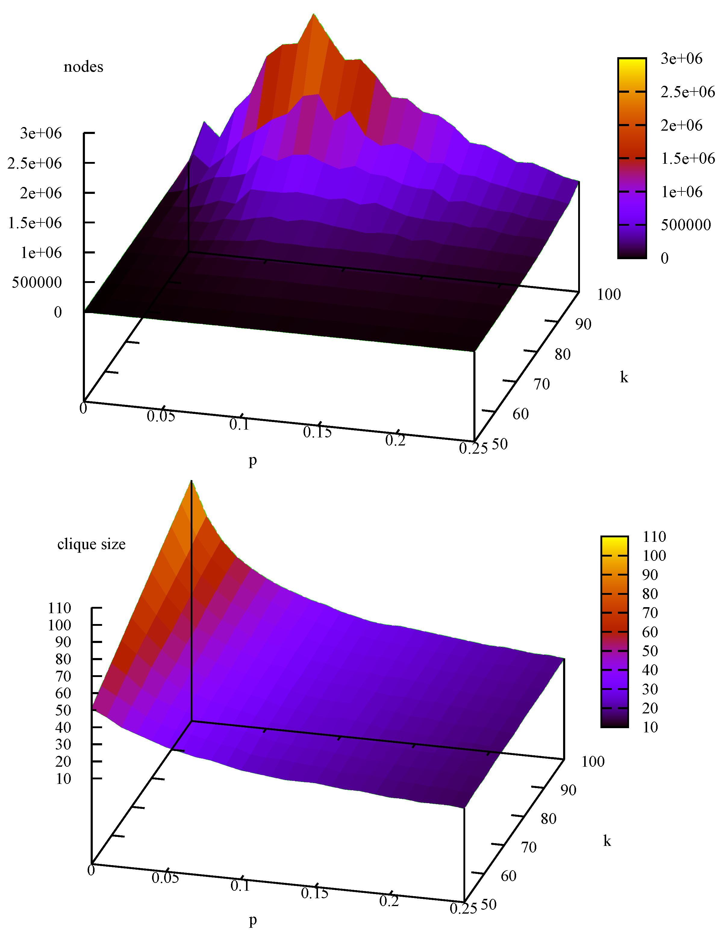
Small world graphs : (upper) search effort, (lower) maximum clique size.

Small-World graphs were then generated using graphgen. This takes three parameters: n the number of vertices, k where each vertex is connected to k nearest neighbours to the right in a ring topology (i.e., vertices start with uniform degree ), and p a rewiring probability. This corresponds to the graphs in Figure 1 of [32]. Small-World graphs were generated with , in steps of 5, in steps of 0.01, 10 graphs at each point. BBMC1 was then applied to each instance to investigate how difficulty of finding a maximum clique varies with respect to k and p and also how size of maximum clique varies, i.e., this is an investigation of the problem. The results are shown as three dimensional plots in Figure 10: The graph above is average search effort and below average maximum clique size. Looking at the graph above: When problems are easy; as p increases and randomness is introduced, the problems quickly get hard, but as p continues to increase the graphs tend to become predominantly random and behave more like large sparse random graphs and get easier. We also see that as neighbourhood size k increases, the problems get harder. We can compare the to the graphs in Table 6: took on average 39,478 nodes whereas took 709,347 nodes, took 2,702,199 nodes and 354,430 nodes. Clearly small-world instances are relatively hard. Looking at the graph below (average maximum clique size), we see that as rewiring probability p increases maximum cliques size decreases, and as k increases so too does maximum clique size.
4.5. Calibration of Results
To compare computational results across publications a standard C program, dfmax, is compiled and run against a set of benchmarks. These run times are then used as a conversion factor, and the results are then taken from one publication, scaled accordingly, and then included in another publication. Recent examples of this are [7] including rescaled results from [33]; [9] including rescaled results from [7], [14] and [4]; [15] including rescaled results from [7] and [33]; [11] including rescaled results from [5]; [10] including rescaled results from [11]; [6] including rescaled results from [9,15]. Is this procedure safe?
To test this we take two additional machines, Fais and Daleview, and calibrate them with respect to our reference machine Cyprus. We then run experiments on each machine using the Java implementations of the algorithms implemented here against some of the DIMACS benchmarks. These results are then rescaled. If the rescaling gives substantially different results from those on the reference machine, this would suggest that this technique is not safe.
| machine | r100.5 | r200.5 | r300.5 | r400.5 | r500.5 | Intel(R) | GHz | cache | Java | scaling factor |
|---|---|---|---|---|---|---|---|---|---|---|
| Cyprus | 0.0 | 0.02 | 0.24 | 1.49 | 5.58 | Xeon(R) E5620 | 2.40 | 12,288KB | 1.6.0_07 | 1 |
| Fais | 0.0 | 0.08 | 0.58 | 3.56 | 13.56 | XEON(TM) CPU | 2.40 | 512KB | 1.5.0_06 | 0.41 |
| Daleview | 0.0 | 0.09 | 0.53 | 3.00 | 10.95 | Atom(TM) N280 | 1.66 | 512KB | 1.6.0_18 | 0.50 |
Table 7 gives a “Rosetta Stone” for the three machines used in this study. The standard program dfmax [37] was compiled using gcc and the -O2 compiler option on each machine and then run on the benchmarks r* on each machine. Run times in seconds are tabulated for the five benchmark instances, each machine’s /proc/cpuinfo is given and a conversion factor relative to the reference machine Cyprus is then computed in the same manner as that reported in [11] (“... the first two graphs from the benchmark were removed (user time was considered too small) and the rest of the times averaged ...”). Therefore when rescaling the run times from Fais, we multiply the actual run time by 0.41 and for Daleview by 0.50.
Table 8 shows the results of the calibration experiments. Tabulated are a subset of DIMACS instances that took more than 1 s and less than 2 h to solve using MCSa1 on our second slowest machine (Fais). Run times are tabulated in milliseconds (in brackets) and the actual ratio of Cyprus-time over Fais-time (expected to be 0.41) is given as well as Cyprus-time over Daleview-time (expected to be 0.50) for each data point. Two algorithms are used, MCSa1 and BBMC1. The last row of Table 8 gives the relative performance ratios computed using the sum of the run times in the table. Referring back to Table 7 we expect a Cyprus/Fais ratio of 0.41 but empirically get 0.12 when using MCSa1 and 0.14 when using BBMC1. We expect a Cyprus/Daleview ratio of 0.50 but empirically get an average 0.26 with MCSa1 and 0.10 with BBMC1. The conversion factors in Table 7 consistently overestimate the speed of Fais and Daleview. For example, we would expect MCSa1 applied to brock200-1 on Fais to have a run time of milliseconds on Cyprus. In fact it takes 4,777 milliseconds. If we use the derived ratio in the last row of Table 8 we get milliseconds. As another example, consider san1000 using BBMC1 on Daleview. We would expect this to take milliseconds on Cyprus. In fact it takes 5,927 milliseconds! If we use the conversion ratio from the last row of Table 8, we get a more accurate estimate milliseconds.
| MCSa1 | BBMC1 | |||||||||||
|---|---|---|---|---|---|---|---|---|---|---|---|---|
| instance | Fais | Daleview | Cyprus | Fais | Daleview | Cyprus | ||||||
| brock200-1 | 0.25 | (19,343) | 0.27 | (17,486) | 1.00 | (4,777) | 0.15 | (15,365) | 0.09 | (25,048) | 1.00 | (2,358) |
| brock200-4 | 0.40 | (1,870) | 0.43 | (1,765) | 1.00 | (755) | 0.20 | (1,592) | 0.13 | (2,464) | 1.00 | (321) |
| hamming10-2 | 0.18 | (1,885) | 0.14 | (2,299) | 1.00 | (333) | 0.25 | (608) | 0.21 | (710) | 1.00 | (151) |
| hamming8-4 | 0.24 | (1,885) | 0.28 | (1,647) | 1.00 | (455) | 0.23 | (1,625) | 0.19 | (1,925) | 1.00 | (367) |
| johnson16-2-4 | 0.35 | (2,327) | 0.38 | (2,173) | 1.00 | (823) | 0.26 | (1,896) | 0.14 | (3,560) | 1.00 | (495) |
| MANN-a27 | 0.21 | (32,281) | 0.22 | (31,874) | 1.00 | (6,912) | 0.14 | (12,335) | 0.10 | (16,491) | 1.00 | (1,676) |
| p-hat1000-1 | 0.25 | (8,431) | 0.28 | (7,413) | 1.00 | (2,108) | 0.14 | (8,359) | 0.12 | (9,389) | 1.00 | (1,169) |
| p-hat1500-1 | 0.19 | (77,759) | 0.22 | (66,113) | 1.00 | (14,421) | 0.11 | (90,417) | 0.10 | (92,210) | 1.00 | (9,516) |
| p-hat300-3 | 0.25 | (53,408) | 0.26 | (51,019) | 1.00 | (13,486) | 0.14 | (41,669) | 0.09 | (60,118) | 1.00 | (5,711) |
| p-hat500-2 | 0.27 | (13,400) | 0.30 | (12,091) | 1.00 | (3,659) | 0.14 | (10,177) | 0.11 | (13,410) | 1.00 | (1,428) |
| p-hat700-1 | 0.40 | (1,615) | 0.51 | (1,251) | 1.00 | (641) | 0.29 | (1,169) | 0.24 | (1,422) | 1.00 | (344) |
| san1000 | 0.11 | (94,107) | 0.12 | (89,330) | 1.00 | (10,460) | 0.10 | (57,868) | 0.11 | (54,816) | 1.00 | (5,927) |
| san200-0.9-1 | 0.29 | (4,918) | 0.31 | (4,705) | 1.00 | (1,444) | 0.18 | (4,201) | 0.11 | (6,588) | 1.00 | (748) |
| san200-0.9-2 | 0.22 | (23,510) | 0.25 | (20,867) | 1.00 | (5,240) | 0.15 | (14,572) | 0.09 | (23,592) | 1.00 | (2,218) |
| san400-0.7-1 | 0.25 | (10,230) | 0.27 | (9,607) | 1.00 | (2,573) | 0.15 | (8,314) | 0.12 | (10,206) | 1.00 | (1,260) |
| san400-0.7-2 | 0.23 | (84,247) | 0.27 | (72,926) | 1.00 | (19,565) | 0.13 | (71,360) | 0.11 | (87,325) | 1.00 | (9,219) |
| san400-0.7-3 | 0.24 | (45,552) | 0.27 | (40,792) | 1.00 | (10,839) | 0.13 | (39,840) | 0.11 | (46,818) | 1.00 | (5,162) |
| sanr200-0.7 | 0.31 | (5,043) | 0.33 | (4,676) | 1.00 | (1,548) | 0.19 | (4,079) | 0.12 | (6,652) | 1.00 | (795) |
| sanr200-0.9 | 0.23 | (1,249,144) | 0.23 | (1,211,762) | 1.00 | (283,681) | 0.15 | (844,487) | 0.09 | (1,409,428) | 1.00 | (123,461) |
| sanr400-0.5 | 0.28 | (9,898) | 0.31 | (8,754) | 1.00 | (2,745) | 0.16 | (9,177) | 0.12 | (12,658) | 1.00 | (1,484) |
| sanr400-0.7 | 0.10 | (7,292,771) | 0.28 | (2,544,196) | 1.00 | (711,861) | 0.14 | (2,698,444) | 0.10 | (3,737,833) | 1.00 | (365,629) |
| ratio (total) | 0.12 | (9,033,624) | 0.26 | (4,202,746) | 1.00 | (1,098,326) | 0.14 | (3,937,554) | 0.10 | (5,622,663) | 1.00 | (539,439) |
But maybe this is because we have used a C program (dfmax) to calibrate a Java program. Would we get a reliable calibration if a C program was used? Östergård’s Cliquer program was downloaded and compiled on our three machines and run against DIMACS benchmarks, i.e., the experiments in Table 8 were repeated using Cliquer and dfmax with a different, and easier, set of problems. The results are shown in Table 9 were an entry “—” was a run of dfmax that was terminated after 2 minutes. What we see is an actual scaling factor of 0.62 for Cliquer on Fais when dfmax predicts 0.41 and for Cliquer on Daleview 0.26 when we expect 0.50; again we see that the rescaling procedure fails. The last three columns show a dfmax calibration using problems other than the r* benchmarks and here we see an error of about 5% on Fais (expected 0.41, actual 0.39) and about 16% on Daleview (expected 0.50, actual 0.43). Therefore, it appears that rescaling results using dfmax and the five r* benchmarks is not a safe procedure and can result in wrong conclusions being drawn regarding the relative performance of algorithms.
4.6. Relative Algorithmic Performance on Different Machines
But is it even safe to draw conclusions on our algorithms when we base those conclusions on experiments performed on a single machine? Previously, in Table 2 we compared MCSa against BBMC on our reference machine Cyprus and concluded that BBMC was typically twice as fast as MCSa. Will that hold on Fais and on Daleview? Table 10 takes the data from Table 8 and divides the run time of MCSa by BBMC for each instance on our three machines. On Fais BBMC is rarely more than 50% faster than MCSa and on Daleview BBMC is slower than MCSa more often than not! If experiments were performed only on Daleview using only the DIMACS instances, we might draw entirely different conclusions and claim that BBMC is slower than MCSa. This change in relative algorithmic ordering has been observed on five different machines (four using the Java 1.6.0) using all of the algorithms. The -server and -client options were also tried. The -server option sometimes gave speedups of a factor of 2, sometimes a factor of 0.5, and this can also affect relative algorithmic performance.
| Cliquer | dfmax | |||||||||||
|---|---|---|---|---|---|---|---|---|---|---|---|---|
| instance | Fais | Daleview | Cyprus | Fais | Daleview | Cyprus | ||||||
| brock200-1 | 0.66 | (9,760) | 0.43 | (18,710) | 1.00 | (6,490) | 0.39 | (25,150) | 0.42 | (23,020) | 1.00 | (9,730) |
| brock200-4 | 0.64 | (690) | 0.47 | (1,190) | 1.00 | (440) | 0.41 | (1,510) | 0.46 | (1,360) | 1.00 | (620) |
| p-hat1000-1 | 0.62 | (1,750) | 0.36 | (3,020) | 1.00 | (1,090) | 0.41 | (1,680) | 0.45 | (1,540) | 1.00 | (690) |
| p-hat700-1 | 0.67 | (150) | 0.37 | (270) | 1.00 | (100) | — | — | — | — | — | — |
| san1000 | 0.75 | (120) | 0.30 | (300) | 1.00 | (90) | — | — | — | — | — | — |
| san200-0.7-1 | 0.48 | (1,750) | 0.20 | (4,220) | 1.00 | (840) | — | — | — | — | — | — |
| san200-0.9-2 | 0.61 | (18,850) | 0.21 | (53,970) | 1.00 | (11,530) | — | — | — | — | — | — |
| san400-0.7-3 | 0.62 | (6,800) | 0.26 | (16,100) | 1.00 | (4,230) | — | — | — | — | — | — |
| sanr200-0.7 | 0.65 | (2,940) | 0.36 | (5,270) | 1.00 | (1,900) | 0.40 | (5,240) | 0.44 | (4,770) | 1.00 | (2,080) |
| sanr400-0.5 | 0.62 | (1,490) | 0.38 | (2,420) | 1.00 | (930) | 0.41 | (3,550) | 0.47 | (3,080) | 1.00 | (1,460) |
| ratio (total) | 0.62 | (44,300) | 0.26 | (105,470) | 1.00 | (27,640) | 0.39 | (37,130) | 0.43 | (33,770) | 1.00 | (14,580) |
5. Conclusions
We have seen that small implementation details (in MC) can result in large changes in performance. Modern programming languages with rich constructs and large libraries of utilities make it easier for the programmer to do this. We have also drifted away from the days when algorithms were presented along with their implementation code (examples here are [8,23]) to presenting algorithms only in pseudo-code. Fortunately we are moving into a new era where code is being made publicly available (examples here are Östergård’s Cliquer and Konc and Janežič’s MaxCliqueDyn) via the web. Hopefully this will grow and allow Computer Scientist to be better able to perform reproducible empirical studies.
Tomita [13] presented MCS as an improvement on MCR brought about via two modifications: (1) a static colour ordering and (2) a colour repair step. Our study has shown that modification (1) improves performance and (2) degrades performance, i.e., MCSa is better than MCSb.
Table 10.
Calibration experiment part 2, does hardware affect relative algorithmic performance? Values greater than 1 imply BBMC is faster than MCSa, and values less than 1 imply MCSa is faster.
| instance | Fais | Daleview | Cyprus |
|---|---|---|---|
| brock200-1 | 1.26 | 0.70 | 2.03 |
| brock200-4 | 1.17 | 0.72 | 2.35 |
| hamming10-2 | 3.10 | 3.24 | 2.21 |
| hamming8-4 | 1.16 | 0.86 | 1.24 |
| johnson16-2-4 | 1.23 | 0.61 | 1.66 |
| MANN-a27 | 2.62 | 1.93 | 4.12 |
| p-hat1000-1 | 1.01 | 0.79 | 1.80 |
| p-hat1500-1 | 0.86 | 0.72 | 1.52 |
| p-hat300-3 | 1.28 | 0.85 | 2.36 |
| p-hat500-2 | 1.32 | 0.90 | 2.56 |
| p-hat700-1 | 1.38 | 0.88 | 1.86 |
| san1000 | 1.63 | 1.63 | 1.76 |
| san200-0.9-1 | 1.17 | 0.71 | 1.93 |
| san200-0.9-2 | 1.61 | 0.88 | 2.36 |
| san400-0.7-1 | 1.23 | 0.94 | 2.04 |
| san400-0.7-2 | 1.18 | 0.84 | 2.12 |
| san400-0.7-3 | 1.14 | 0.87 | 2.10 |
| sanr200-0.7 | 1.24 | 0.70 | 1.95 |
| sanr200-0.9 | 1.48 | 0.86 | 2.30 |
| sanr400-0.5 | 1.08 | 0.69 | 1.85 |
| sanr400-0.7 | 2.70 | 0.68 | 1.95 |
BBMC is algorithm MCSa with sets represented as bit strings, i.e., BitSet is used rather than ArrayList. Experiments on the reference machine showed a speedup typically of a factor of 2. The three styles of ordering were investigated. The orderings were quickly disrupted by MCQ, but in the other algorithms minimum width ordering was the best in random problems, whereas in the DIMACS instances there was no clear winner.
New benchmark problems (i.e., problems rarely investigated by the maximum clique community) were investigated such as BHOSLIB, k-regular and small-world graphs. Motivation for this study was partly to compare algorithms but also to explore these problems to determine if and when they are hard.
Finally, we demonstrated that the standard procedure for calibrating machines and rescaling results is unsafe, and that running our own code on different machines can lead to different relative algorithmic performance. This is disturbing. First, it suggests that to perform a fair and reliable empirical study we should not rescale others’ results: We must either code up the algorithms ourselves, as done here and also by Carmo and Züge [2], or download and run code on our machines. Secondly, we should run our experiments on different machines.
All the codes used in this study are available online [34] along with instructions on how to run the code, the DIMACS instances, random problem generator and runtime results.
Appendix
At the top of MCQ’s search, Tomita [12] sorts vertices in non-increasing degree order and the first Δ vertices are given colours 1 to Δ respectively, where Δ is the maximum degree in the graph, thereafter vertices are given colour . This is done to prime the candidate set for the initial call to EXPAND. Thereafter Tomita calls NUMBER-SORT immediately before the recursive call to EXPAND. A simpler option is taken here: colouring and sorting of the candidate set is done only at the start of . Using graph g10–50 as an example, in Figure 2 of [12] vertices would initially be selected in the order [7,9,8,5,2,1,6,4,0,3] with colours respectively [6,6,6,6,6,5,4,3,2,1], i.e., using 6 colours. Here vertices are selected in order [9,8,5,7,2,1,6,4,0,3] with colours [4,3,3,2,2,2,2,1,1,1], i.e., using 4 colours, a tighter upper bound and vertices no longer in degree order.
Figure 11.
The effect of Tomita’s initial colour ordering.

Listing 13 presents a Java implementation of MCQ as described in [12] but in our framework. Lines 18 to 20 give an initial colour to the sorted vertices. Method is now called after the selection of a vertex (line 40). A similar change was made to MCSa. Figure 11 shows the effect of the initial colour ordering, using on calls to (nodes). We see on the left that Tomita’s MCQ is marginally better than MCQ1 and on the right that MCSa1 is better than Tomita’s equivalent (and we see a similar improvement in BBMC1). In conclusion, the approach adopted here is simpler, using a single colour-ordering procedure. In MCQ1 the effect on performance is detrimental but small, and in MCSa1 (and BBMC1a) it is beneficial.
Acknowledgements
I would like to thank Pablo San Segundo, Jeremy Singer, Ciaran McCreesh and my reviewers.
Listing 13. MCQTomita.

References
- Garey, M.R.; Johnson, D.S. Computers and Intractability; W.H. Freeman and Co.: New York, NY, USA, 1979. [Google Scholar]
- Renato, C.; Alexandre, P. Z. Branch and bound algorithms for the maximum clique problem under a unified framework. J. Braz. Comp. Soc. 2012, 18, 137–151. [Google Scholar]
- Randy, C.; Panos, M.P. An exact algorithm for the maximum clique problem. Oper. Res. Lett. 1990, 9, 375–382. [Google Scholar]
- Torsten, F. Simple and Fast: Improving a Branch-and-Bound Algorithm for Maximum Clique. In Proceedings of the ESA 2002, LNCS 2461, Rome, Italy, 17–21 September 2002; pp. 485–498.
- Janez, K.; Dušanka, J. An improved branch and bound algorithm for the maximum clique problem. MATCH Commun. Math. Comput. Chem. 2007, 58, 569–590. Available online: http://www.sicmm.org/ konc/ (accessed on 12 November 2012). [Google Scholar]
- Chu, M.; Li, Z.Q. An Efficient Branch-and-Bound Algorithm Based on Maxsat for the Maximum Clique Problem. In Proceedings of the AAAI’10, Atlanta, GA, USA, 11–15 July 2010; pp. 128–133.
- Östergård, P.R.J. A fast algorithm for the maximum clique problem. Discret. Appl. Math. 2002, 120, 197–207. Available online: http://users.tkk.fi/pat/cliquer.html/ (accessed on 12 November 2012). [Google Scholar] [CrossRef]
- Pardalos, P.M.; Rodgers, G.P. A branch and bound algorithm for the maximum clique problem. Comput. Oper. Res. 1992, 19, 363–375. [Google Scholar] [CrossRef]
- Régin, J.-C. Using Constraint Programming to Solve the Maximum Clique Problem. In Proceedings CP 2003, LNCS 2833, Kinsale, Ireland, 29 September–3 October 2003; pp. 634–648.
- Segundo, P.S.; Matia, F.; Diego, R.-L.; Miguel, H. An improved bit parallel exact maximum clique algorithm. Optim. Lett. 2011. [Google Scholar] [CrossRef]
- Segundo, P.S.; Diego, R.-L.; Augustín, J. An exact bit-parallel algorithm for the maximum clique problem. Comput. Oper. Res 2011, 38, 571–581. [Google Scholar] [CrossRef]
- Tomita, E.; Sutani, Y.; Higashi, T.; Takahashi, S.; Wakatsuki, M. An Efficient Branch-and-Bound Algorithm for Finding a Maximum Clique. In Proceedings of the DMTCS 2003, LNCS 2731, Dijon, France, 7–12 July 2003; pp. 278–289.
- Tomita, E.; Sutani, Y.; Higashi, T.; Takahashi, S.; Wakatsuki, M. A Simple and Faster Branch-and-Bound Algorithm for Finding Maximum Clique. In Proceedings of the WALCOM 2010, LNCS 5942, Dhaka, Bangladesh, 10–12 February 2010; pp. 191–203.
- Wood, D.R. An algorithm for finding a maximum clique in a graph. Oper. Res. Lett. 1997, 21, 211–217. [Google Scholar] [CrossRef]
- Tomita, E.; Toshikatsu, K. An efficient branch-and-bound algorithm for finding a maximum clique and computational experiments. J. Glob. Optim. 2007, 37, 95–111. [Google Scholar] [CrossRef]
- David, E.; Darren, S. Listing all maximal cliques in large sparse real-world graphs. Experimental Algorithms, LNCS 6630. Comput. Sci. 2011, 6630, 364–375. [Google Scholar]
- Knuth, D.E. Generating all Combinations and Permutations. In The Art of Computer Programming; Pearson Education Inc.: Stoughton, MA, USA, January 2006; Volume 4, pp. 1–3. [Google Scholar]
- Li, C.M.; Quan, Z. Combining Graph Structure Exploitation and Propositional Reasoning for the Maximum Clique Problem. In Proceedings of the ICTAI’10, Arras, France, 27–29 October 2010; Volume 1, pp. 344–351.
- Bentley, J.L.; McIlroy, M.D. Engineering a sort function. Softw.-Pract. Exp. 1993, 23, 1249–1265. [Google Scholar] [CrossRef]
- Eugene, C.F. A sufficient condition for backtrack-free search. J. Assoc. Comput. Mach. 1982, 29, 24–32. [Google Scholar]
- David, W.M.; Beck, L.L. Smallest-Last ordering and clustering and graph coloring algorithms. J. Assoc. Comput. Mach. 1983, 30, 417–427. [Google Scholar]
- Pardalos, P.M.; Xue, J. The maximum clique problem. J. Glob. Optim. 1994, 4, 301–324. [Google Scholar] [CrossRef]
- Bron, C.; Kerbosch, J. Algorithm 457: Finding all cliques of an undirected graph [h]. Commun. ACM 1973, 16, 575–579. [Google Scholar] [CrossRef]
- Akkoyunlu, E.A. The enumeration of maximal cliques of large graphs. SIAM J. Comput. 1973, 2, 1–6. [Google Scholar] [CrossRef]
- Tomita, E.; Tanaka, A.; Takahashi, H. The worst-case time complexity for generating all maximal cliques and computational experiments. Theor. Comput. Sci. 2006, 363, 28–42. [Google Scholar] [CrossRef]
- Abu-Khzam, F.N.; Collins, R.L.; Fellows, M.R.; Langston, M.A.; Suters, W.H.; Symons, C.T. Kernelization algorithms for the vertex cover problem: Theory and experiments. In ALENEX/ANALC, New Orleans, LA, USA, 10–13 January 2004; pp. 62–69.
- Segundo, P.S.; Tapia, C. A New Implicit Branching Strategy for Exact Maximum Clique. In Proceedings of ICTAI’10, Arras, France, 27–29 October 2010; Volume 1, pp. 352–357.
- Cheeseman, P.; Kanefsky, B.; Taylor, W.M. Where the Really Hard Problems are. In Proceedings of the IJCAI’91, Sidney, Australia, 24–30 August 1991; pp. 331–337.
- Gent, I.P.; MacIntyre, E.; Prosser, P.; Walsh, T. The Constrainednss of Search. In Proceedings of the AAAI’96, Portland, OR, USA, 4–8 August 1996; pp. 246–252.
- Zweig, K.A.; Palla, G.; Vicsek, T. What makes a phase transition? Analysis of the random satisfiability problem. Physica A 2010, 389, 1501–1511. [Google Scholar]
- DIMACS instances. Available online: ftp://dimacs.rutgers.edu/pub/challenge/graph/benchmarks/clique (accessed on 12 November 2012).
- Watts, D.J.; Strogatz, S.H. Collective dynamics of small world networks. Nature 1998, 394, 440–442. [Google Scholar] [CrossRef] [PubMed]
- Sewell, E.C. A branch and bound algorithm for the stability number of a sparse graph. INFORMS J. Comput. 1998, 10, 438–447. [Google Scholar] [CrossRef]
- Prosser, P. Maximum Clique Algorithms in Java. Available online: http://www.dcs.gla.ac.uk/ pat/maxClique (accessed on 12 November 2012).
- Stanford Large Network Dataset Collection. Available online: http://snap.stanford.edu/data/index.html (accessed on 12 November 2012).
- Benchmarks with Hidden Optimum Solutions. Available online: http://www.nlsde.buaa.edu.cn/kexu/benchmarks/graph-benchmarks.htm (accessed on 12 November 2012).
- Dfmax. Available online: ftp://dimacs.rutgers.edu/pub/dsj/clique (accessed on 12 November 2012).
© 2012 by the author; licensee MDPI, Basel, Switzerland. This article is an open access article distributed under the terms and conditions of the Creative Commons Attribution license (http://creativecommons.org/licenses/by/3.0/).
Share and Cite
MDPI and ACS Style
Prosser, P. Exact Algorithms for Maximum Clique: A Computational Study . Algorithms 2012, 5, 545-587. https://doi.org/10.3390/a5040545
AMA Style
Prosser P. Exact Algorithms for Maximum Clique: A Computational Study . Algorithms. 2012; 5(4):545-587. https://doi.org/10.3390/a5040545
Chicago/Turabian StyleProsser, Patrick. 2012. "Exact Algorithms for Maximum Clique: A Computational Study " Algorithms 5, no. 4: 545-587. https://doi.org/10.3390/a5040545