Department of Neurobiology, Weizmann Institute of Science, Rehovot, Israel
Analysis of multichannel recordings acquired with contemporary imaging or electrophysiological methods in neuroscience is often difficult due to the high dimensionality of the data and the low signal-to-noise ratio. We developed a method that addresses both problems by utilizing prior information about the temporal structure of the signal and the noise. This information is expressed mathematically in terms of sets of correlation matrices, a versatile approach that allows the treatment of a large class of signal and noise sources, including non-stationary sources or correlated signal and noise sources. We present a mathematical analysis of the algorithm, as well as application to an artificial dataset, and show that the algorithm is tolerant to inaccurate assumptions about the temporal structure of the data. We suggest that the algorithm, which we name temporally structured component analysis, can be highly beneficial to various multichannel measurement techniques, such as fMRI or optical imaging.
Contemporary methods in neuroscience research, ranging from multielectrode recordings, through optical imaging, to fMRI, EEG and MEG allow the collection of large volumes of multichannel data in a single experiment. Such data can be highly informative about the underlying neuronal machinery, as it can reveal its rich and complex dynamics, as well as its spatial structure. However, this data is inherently difficult to analyze due to two fundamental issues (Mitra and Pesaran, 1999
). First, there are problems associated with the nature of high dimensional structures, such as the difficulty to visualize them or to fit them with statistical models. Second, the signal-to-noise ratio is often very low. A typical example for the latter problem is when the signal, which is identified with neuronal activity, is masked by strong non-neuronal sources, which are considered noise. In this contribution however we deal with the signal-to-noise ratio problem from a broader perspective: we view the signal as any aspect of the data that is of interest in a particular context; everything else is considered noise.
A general approach for analyzing multichannel data is to reduce its dimensionality. Since in many neuroscientific measurements the different channels are correlated, the data is redundant, and its dimensionality can be reduced without causing a significant loss of information. Moreover, one can seek a low dimensional representation that retains the signal’s structure but suppresses the noise. If such a representation is attainable, the new representation not only exhibits an improved signal-to-noise ratio but is also easier to analyze, merely due to its reduced dimensionality.
Out of the numerous dimensionality reduction methods, one of the simplest and most popular is principal component analysis (PCA; e.g., Jolliffe, 2002
)
1
. In PCA, the multichannel measurement at time t, z(t), is approximated by a linear sum of basis vectors ψ1, ψ2,…called “principal components”, i.e.,  The principal components ψi are selected such that they maximize an objective function defined as the power of the associated time course of the coefficients αi(t). Moreover, the n components with maximal power provide the best linear approximation of the data using n components in a well-defined mathematical sense. For neuroscientific measurements, which are typically redundant, a small number of components suffice for approximating the data, and the dimensionality can be dramatically reduced.
The principal components ψi are selected such that they maximize an objective function defined as the power of the associated time course of the coefficients αi(t). Moreover, the n components with maximal power provide the best linear approximation of the data using n components in a well-defined mathematical sense. For neuroscientific measurements, which are typically redundant, a small number of components suffice for approximating the data, and the dimensionality can be dramatically reduced.While highly successful in dimensionality reduction, PCA often performs poorly in terms of separating the signal from the noise. It is rarely the case that a particular principal component can be associated solely with the signal, and it is much more common that the principal components are “non-interpretable” and reflect useless mixtures of signal and noise. As a result, PCA is often disregarded as a rigorous method for data analysis. We observe that both the success of PCA in dimensionality reduction and its failure in separating the signal from the noise follow from the PCA objective function. While maximizing the power guarantees an optimal low dimensional representation, this objective function is completely “blind” to the fact that data combines a signal, which is of interest, and a noise, which should be suppressed. Moreover, the PCA construction is ignorant to the fact that the data constitutes a multidimensional time-series, in which the samples, i.e., measurements at different points in time, are correlated.
In this contribution we propose an algorithm suitable for the analysis of multichannel measurements. We refer to the algorithm as “temporally structured components analysis” (TSCA). The algorithm adheres to the PCA framework by seeking components with high power. However, in order to avoid the mixing of the signal and the noise, it seeks components that maximize the power originating from the signal while minimizing power arising from the noise. The main challenge here is to tell apart the signal from the noise. We address this problem by making use of the fact that the signal and the noise typically have different temporal structures, and that prior information about their temporal characteristics is often at hand. For example, neuronal responses evoked by a stimulus can be characterized by their expected timing within the recording, which is set by the stimulation protocol, and by quantities such as the neural delay, which can be estimated. Another example is the approximately periodic artifacts originating from heartbeat pulsation. These artifacts can be characterized by their fundamental frequency, which can be measured independently or estimated from the data. In both cases, the information required for the characterization of the signal and the noise is either known a-priori, or can be estimated.
In the following sections we show how the prior temporal information can be systematically incorporated in a PCA-like framework. The main building block of the mathematical construction is the expression of the prior information in terms of correlation matrices, i.e., matrices of second order moments of the signal and the noise. This definition is very versatile, and allows the treatment of a very broad class of signal or noise sources, as well as dealing with statistical dependencies between the signal and the noise.
Our goal in this contribution is to present the algorithm and the theoretical construction underlying it. To this end, we first provide the mathematical derivation of the algorithm for a simplified case that captures the essence of the algorithm. Then, we discuss some results for the general case (full analysis is presented in Section 1 and 2 of the Supplementary Material). We next present simulation results to validate the algorithm, and to demonstrate some of its additional properties, such as robustness to errors in the assumed temporal structure of the data. We finish with a discussion, focusing on how the algorithm can be applied in practical cases, and on comparison with other algorithms.
Analysis of a Simplified Case
We consider the data to be a matrix Z with dimensions P times T, where P is the number of channels and T is the number of time samples. The matrix Z is stochastic (i.e., Z is a matrix-valued random variable), and constitutes a multidimensional time-series. A basic operation in the analysis is to transform Z into a one-dimensional time-series by projecting it onto a P-dimensional unit vector ψ, an operation written as ψTZ. One measure of the importance or dominance of a particular direction ψ is the expected power of ψTZ, a quantity we write as  where E(·) denotes expectation taken over realizations of Z. The approach taken by PCA is to find components ψ such that
  is maximized. The solution to this maximization problem is given by eigenvectors of the theoretical covariance matrix, which is given, up to a scaling, by E(ZZT). In practice, the theoretical covariance matrix is replaced by the empirical covariance matrix, estimated from the observations.
where E(·) denotes expectation taken over realizations of Z. The approach taken by PCA is to find components ψ such that is maximized. The solution to this maximization problem is given by eigenvectors of the theoretical covariance matrix, which is given, up to a scaling, by E(ZZT). In practice, the theoretical covariance matrix is replaced by the empirical covariance matrix, estimated from the observations.We further assume the matrix Z to be the sum of a signal X and a noise Y, i.e., Z = X + Y. Since PCA maximizes  , it is not guaranteed, in general, that the power of the projection of the signal on ψ, i.e.,
  , is high. Our approach is to replace the maximization of the PCA objective function with either the maximization of
  , the minimization of
  , or an interplay between these two objectives. Clearly, neither the maximization of
  nor the minimization of
  can be done directly, because neither X nor Y are observed; only their sum Z is known.
, it is not guaranteed, in general, that the power of the projection of the signal on ψ, i.e., , is high. Our approach is to replace the maximization of the PCA objective function with either the maximization of , the minimization of , or an interplay between these two objectives. Clearly, neither the maximization of nor the minimization of can be done directly, because neither X nor Y are observed; only their sum Z is known.We will develop a solution to this problem by studying a simplified but instructive case. We assume the signal to be a multidimensional process with a fixed spatial structure whose amplitude fluctuates according to a stochastic process. Thus, we express X as X = uXaX where the spatial component uX is a fixed, length P, column vector, and aX is a stochastic process, represented by a length T row vector (note that throughout the manuscript column vectors are used for space, and row vectors are used for time). We choose the noise to be of a similar form Y = uYaY, with uY being fixed and aY stochastic. No particular assumptions about the probability distribution of aX are made, but for the noise we assume that it is statistically independent of the signal and has zero mean in all its entries, i.e., E(aY) = 0. Our approach for maximizing  assumes that some prior knowledge about the temporal structure of the signal and the noise is available. Specifically, we require that the autocorrelation matrices of the signal and the noise are known, up to scaling. We denote these matrices by CX and CY, and define them respectively by E(aX T aX) and E(aY T aY). These matrices are of size T × T. For CX (or CY), the entry at row t, column t′, measures the correlation between the value of the signal (or the noise) at times t and t′.
assumes that some prior knowledge about the temporal structure of the signal and the noise is available. Specifically, we require that the autocorrelation matrices of the signal and the noise are known, up to scaling. We denote these matrices by CX and CY, and define them respectively by E(aX T aX) and E(aY T aY). These matrices are of size T × T. For CX (or CY), the entry at row t, column t′, measures the correlation between the value of the signal (or the noise) at times t and t′.An example of such data is given in Figure 1
A. The signal X has a fixed spatial component uX, which we chose, rather arbitrarily, to be an image of a circle in a square frame (left top). The random vector aX, which defines the temporal evolution of the signal, was selected to mimic the time course of a stimulus-triggered response. The response starts at times 0,100,…,900. It has a constant exponential shape, but variable amplitude. A particular realization of aX is shown on the right. The noise Y was constructed with a sinusoidal-gratings spatial component (uY, Figure 1
A, left bottom). Its time course was defined by an autoregressive process of order 5, for which we show a particular realization on the right. The observed data Z is constructed summing X and Y, so every frame is a linear combination of the circle and the gratings (Figure 1
B). The autocorrelation matrices for the signal and the noise processes are shown in Figure 1
C (left: CX, right: CY). Intuitively, analysis of the signal requires the recovery of the circle image uX from the data Z. This intuition is met by the mathematical formulation presented above, because  is maximized when ψ = uX.
is maximized when ψ = uX.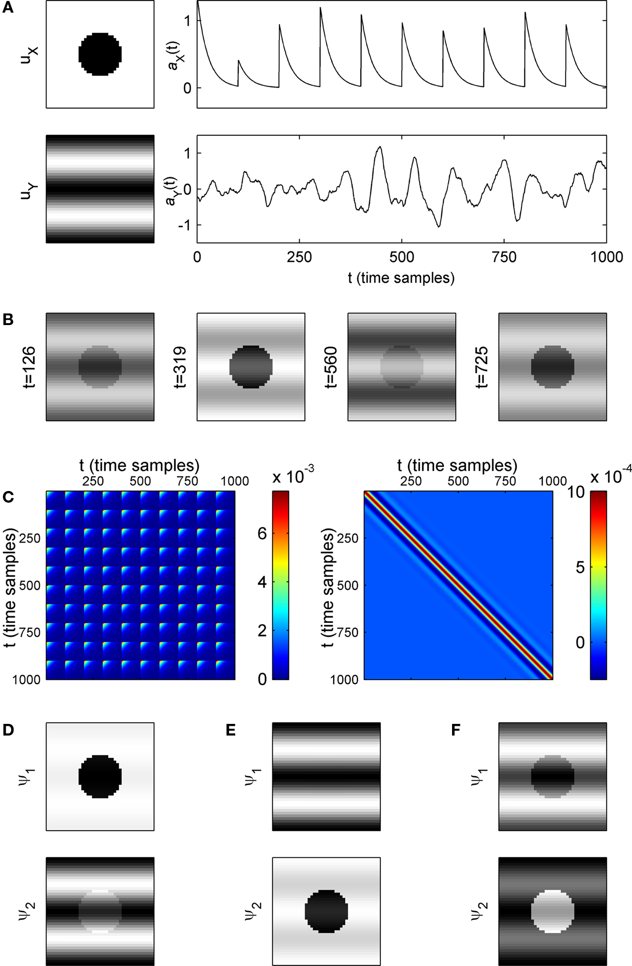
Figure 1. Application of the algorithm on simple artificial data. (A) Construction of the data. The signal (top) and the noise (bottom) have fixed spatial components (uX and uY, correspondingly), which are normalized to have unit norm. The time course for the signal is determined by a stochastic process:  with g(t) = Θ(t)e−t/25, Θ(·) being the Heaviside step function, and rl denoting random variables independently drawn from a Gaussian distribution N(1, 0.0625). The time course for the noise is an AR(5) process: aY(t) = 1.2aY(t − 1) − 0.215aY(t − 5) + ε(t), with ε(t) independently drawn from a Gaussian distribution N(0, 0.0008). The standard deviation of ε(t) was selected such that the power of aY matches approximately the power of aX. A particular realization of these processes is shown on the right. The data at time t is constructed by a linear sum: aX(t)uX + aY(t)uY. (B) Examples of data frames. (C) Autocorrelation matrix of the signal (left) and the noise (right). (D) Spatial components extracted by TSCA. The first spatial component is similar to uX. (E) Spatial components extracted by TSCA with the signal and noise switched. The first spatial component is now similar to uY. (F) Spatial components extracted by PCA. Unlike the results from TSCA, here the first principal component is a mixture of uX and uY.
with g(t) = Θ(t)e−t/25, Θ(·) being the Heaviside step function, and rl denoting random variables independently drawn from a Gaussian distribution N(1, 0.0625). The time course for the noise is an AR(5) process: aY(t) = 1.2aY(t − 1) − 0.215aY(t − 5) + ε(t), with ε(t) independently drawn from a Gaussian distribution N(0, 0.0008). The standard deviation of ε(t) was selected such that the power of aY matches approximately the power of aX. A particular realization of these processes is shown on the right. The data at time t is constructed by a linear sum: aX(t)uX + aY(t)uY. (B) Examples of data frames. (C) Autocorrelation matrix of the signal (left) and the noise (right). (D) Spatial components extracted by TSCA. The first spatial component is similar to uX. (E) Spatial components extracted by TSCA with the signal and noise switched. The first spatial component is now similar to uY. (F) Spatial components extracted by PCA. Unlike the results from TSCA, here the first principal component is a mixture of uX and uY.In order to (indirectly) maximize  or minimize
  based on the data Z, we will first try to estimate these quantities for a fixed ψ. To this end, we consider a quadratic estimator of the form:
or minimize based on the data Z, we will first try to estimate these quantities for a fixed ψ. To this end, we consider a quadratic estimator of the form:
where Q is an arbitrary symmetric T × T matrix. Our goal now is to constrain Q such that mQ(ψ) will enable us to estimate 
 or some combination of them. Thus, we calculate the expectation (taken over realizations) of mQ(ψ), and express it in terms of
  and
and  . We find that:
or some combination of them. Thus, we calculate the expectation (taken over realizations) of mQ(ψ), and express it in terms of and . We find that:
where  is the matrix inner product. Eq. 2 implies that mQ(ψ) is an unbiased estimator for a weighted sum of
  and
and  that takes the form:
is the matrix inner product. Eq. 2 implies that mQ(ψ) is an unbiased estimator for a weighted sum of and that takes the form:
Moreover, Eqs. 2 and 3 together imply that if we know CX and CY up to a scaling factor, then expressions of the form given by Eq. 3 can be estimated for any γX and γY, by finding Q such that:

Expressions of the form in Eq. 3 are useful objective functions. For example, choosing γX = 1, γY = 0, produces an estimator of  . A direct calculation shows that this objective function is maximized for ψ = uX. Thus, the maximization of m(ψ) with γX = 1, γY = 0, is a strategy for recovering uX from the data. Another choice which is of interest is γX = 0 and γY = −1. When this expression is maximized,
  is minimized, and more generally, a tradeoff between maximizing
  and minimizing
  follows when selecting γX = 1 and γY < 0. Later, we address how the value of γY affects the solution of the optimization problem, but for now, we restrict neither γX nor γY.
. A direct calculation shows that this objective function is maximized for ψ = uX. Thus, the maximization of m(ψ) with γX = 1, γY = 0, is a strategy for recovering uX from the data. Another choice which is of interest is γX = 0 and γY = −1. When this expression is maximized, is minimized, and more generally, a tradeoff between maximizing and minimizing follows when selecting γX = 1 and γY < 0. Later, we address how the value of γY affects the solution of the optimization problem, but for now, we restrict neither γX nor γY.Eq. 4 constitute a linear system with two equations and (T + 1)T/2 variables (the number of independent entries in the symmetric matrix Q). Unless CX and CY are the same up to a scaling factor and therefore are linearly dependent, an infinite number of solutions exists for any selection of γX and γY. This degeneracy can be utilized to minimize the variance of the estimator mQ(ψ). In general, this variance cannot be expressed only in terms of the correlation matrices, as it depends on moments of Z of order higher than 2. So as not to require knowledge of higher order moments, we use an upper bound obtained by applying the Cauchy-Schwarz inequality to the variance (Eq. A12, see Section 1 of the Supplementary Material). This bound holds for any Q satisfying Eq. 4, and is given by:

where ||Q||2 = tr(QTQ) is the squared Frobenius norm. Since the bound depends on Q only through the factor ||Q||2, a reasonable strategy for minimizing the estimation variance is simply to minimize ||Q||2. Given CX, CY, γX, and γY, the solution for Eq. 4 with minimal ||Q||2 is a linear combination of CX and CY given by:
Having derived an expression for Q, we can estimate m(ψ) by mQ(ψ), and therefore we can treat m(ψ) as an objective function to be maximized over all ψ’s. The solution to this maximization problem is analogous to the PCA solution. Here, it is given by eigenvectors of ZQZT, and the eigenvalue of a particular eigenvector ψi is equal to the estimate of m(ψi). If we sort the eigenvectors according to their eigenvalues in a descending order, the first eigenvector obtains the global maximum of the objective function; the second eigenvector obtains the maximum in the subspace orthogonal to the first eigenvector; and so forth.
Based on the analysis above, we can summarize the basic algorithm. First, we select an objective function m(ψ) of the form in Eq. 3 by choosing γX and γY. Using prior knowledge of the autocorrelation of the signal CX and the noise CY we construct the estimator for m(ψ) by calculating Q according to Eq. 6. We then diagonalize ZQZT and sort the eigenvectors according to their eigenvalues. Those with highest eigenvalues maximize the objective function.
We demonstrate this procedure on the data in Figure 1
. We selected the objective function by choosing γX = 1, γY = 0, so the objective function is simply  . Then, Q was calculated using the autocorrelation matrices in Figure 1
C. Applying the algorithm for the realization of Z in Figure 1
A, we diagonalized ZQZT. The first eigenvector ψ1 is shown in Figure 1
D, top panel. It is highly similar to the spatial component of the signal
. Then, Q was calculated using the autocorrelation matrices in Figure 1
C. Applying the algorithm for the realization of Z in Figure 1
A, we diagonalized ZQZT. The first eigenvector ψ1 is shown in Figure 1
D, top panel. It is highly similar to the spatial component of the signal  The algorithm therefore successfully recovered the spatial component of the signal, as desired by this choice of objective function. In this simplified example all columns of Z belong to the two dimensional linear subspace spanned by uX and uY. The rank of Z is therefore 2, and there is only one more non-zero eigenvalue. The corresponding eigenvector is shown at the bottom of Figure 1
D. Note that if we were interested in the spatial component of the noise, we could still use TSCA by switching the roles of the signal and the noise. Applying the algorithm this way produces the eigenvectors in Figure 1
E. Now, the first eigenvector (top) corresponds to the noise spatial component
The algorithm therefore successfully recovered the spatial component of the signal, as desired by this choice of objective function. In this simplified example all columns of Z belong to the two dimensional linear subspace spanned by uX and uY. The rank of Z is therefore 2, and there is only one more non-zero eigenvalue. The corresponding eigenvector is shown at the bottom of Figure 1
D. Note that if we were interested in the spatial component of the noise, we could still use TSCA by switching the roles of the signal and the noise. Applying the algorithm this way produces the eigenvectors in Figure 1
E. Now, the first eigenvector (top) corresponds to the noise spatial component  For comparison, we applied PCA on the same data. This resulted in the usual mixing of the signal and noise (Figure 1
F;
For comparison, we applied PCA on the same data. This resulted in the usual mixing of the signal and noise (Figure 1
F;  ). This phenomenon can be understood using the formulation developed above: PCA is obtained by selecting Q to be the identity matrix. Plugging Q = I in Eq. 2, and observing that
  we see that the quantity maximized in this case is
  which cannot be expected to appropriately separate the signal from the noise.
. Then, Q was calculated using the autocorrelation matrices in Figure 1
C. Applying the algorithm for the realization of Z in Figure 1
A, we diagonalized ZQZT. The first eigenvector ψ1 is shown in Figure 1
D, top panel. It is highly similar to the spatial component of the signal The algorithm therefore successfully recovered the spatial component of the signal, as desired by this choice of objective function. In this simplified example all columns of Z belong to the two dimensional linear subspace spanned by uX and uY. The rank of Z is therefore 2, and there is only one more non-zero eigenvalue. The corresponding eigenvector is shown at the bottom of Figure 1
D. Note that if we were interested in the spatial component of the noise, we could still use TSCA by switching the roles of the signal and the noise. Applying the algorithm this way produces the eigenvectors in Figure 1
E. Now, the first eigenvector (top) corresponds to the noise spatial component For comparison, we applied PCA on the same data. This resulted in the usual mixing of the signal and noise (Figure 1
F; ). This phenomenon can be understood using the formulation developed above: PCA is obtained by selecting Q to be the identity matrix. Plugging Q = I in Eq. 2, and observing that we see that the quantity maximized in this case is which cannot be expected to appropriately separate the signal from the noise.The General Case
The analysis presented above makes the rather strong assumption that both the signal and the noise have one, fixed, spatial component, and that they are uncorrelated. Clearly, these assumptions are unrealistic for complex biological data. However, using mathematical principles similar to the ones presented above, we can generalize the algorithm such that the restrictive assumptions are replaced by weaker ones. Detailed discussion is presented in Section 1 and 2 of the Supplementary Material. Here, we briefly sketch the generalized formulation and summarize the main results. We clearly state the underlying assumptions, which define the algorithms’ scope of applicability.
In the general case, we assume that the data Z originates from NX signal sources  and NY noise sources
  , which combine additively. Each of the sources is an arbitrary matrix valued random variable. The objective function is generalized and takes the form:
  As before, the free parameters of the objective function γX and γY control a tradeoff between maximizing signal power, now given by
  and minimizing noise power, i.e.,
  . The estimation of the objective function is obtained by using an unbiased estimator mQ(ψ) of the form given by Eq. 1, with Q being a linear combination of correlation matrices (Eqs. A13 and A14, Section 1 of the Supplementary Material). The maximization of mQ(ψ) is solved by diagonalizing ZQZT, and the leading eigenvectors of ZQZT maximize the objective function, as in the simplified case.
and NY noise sources , which combine additively. Each of the sources is an arbitrary matrix valued random variable. The objective function is generalized and takes the form: As before, the free parameters of the objective function γX and γY control a tradeoff between maximizing signal power, now given by and minimizing noise power, i.e., . The estimation of the objective function is obtained by using an unbiased estimator mQ(ψ) of the form given by Eq. 1, with Q being a linear combination of correlation matrices (Eqs. A13 and A14, Section 1 of the Supplementary Material). The maximization of mQ(ψ) is solved by diagonalizing ZQZT, and the leading eigenvectors of ZQZT maximize the objective function, as in the simplified case.The main difference between the simplified and general cases is the definition of the correlation matrices. Whereas in the simplified case there was one correlation matrix for the signal and one correlation matrix for the noise, in the general case there are three sets of matrices: (1) Signal correlation matrices, representing the temporal correlations within each of the signal sources; (2) Noise correlation matrices representing the temporal correlations within each of the noise sources; and (3) Interaction correlation matrices, accounting for potential correlations between the different signal and noise sources. In order to define these matrices, we consider a decomposition of each of the signal and noise sources: Xj = UXjAXj and Yj = UYjAYj. Here, each matrix UXj, UYj is a fixed matrix of size P by  or P by
  , respectively, and each of the matrices AXj, AYj is a matrix valued random variable of compatible size. The number of columns in UXj, UYj, i.e.,
  or
or  , is arbitrary, although having a decomposition with small
  and
and  simplifies the actual calculation of the correlation matrices. Note that there is always an infinite number of such decompositions for each source, as UXj or UYj can be defined as any invertible matrix, and AXj, AYj as the inverse of that matrix multiplied by Xj or Yj. However, the precise choice of UXj, AXj, UYj and AYj is not important because all choices lead to a valid matrix Q. Moreover, all choices of UXj, UYj such that their columns are linearly independent are equivalent, and lead to precisely the same matrix Q. Using these decompositions the definition of the signal, noise, and interaction correlation matrices is, respectively, the set of symmetrized expected outer products between any two rows of (1) the same matrix in the set {AXj}, (2) the same matrix in the set {AYj}, and (3) different matrices in the set {AXj} ∪ {AYj} (see Eq. A3, Section 1 of the Supplementary Material). In order to construct Q however, it is sufficient to know only arbitrary bases for the linear span of the three set of matrices (see Eq. A10, Section 1 of the Supplementary Material). In particular, it follows that similarly to the simplified case, it is enough to know the correlation matrices only up to a scaling factor. Note also that the definitions of the correlation matrices reduce to the definitions of the simplified case whenever the conditions for the simplified case are satisfied.
or P by , respectively, and each of the matrices AXj, AYj is a matrix valued random variable of compatible size. The number of columns in UXj, UYj, i.e., or , is arbitrary, although having a decomposition with small and simplifies the actual calculation of the correlation matrices. Note that there is always an infinite number of such decompositions for each source, as UXj or UYj can be defined as any invertible matrix, and AXj, AYj as the inverse of that matrix multiplied by Xj or Yj. However, the precise choice of UXj, AXj, UYj and AYj is not important because all choices lead to a valid matrix Q. Moreover, all choices of UXj, UYj such that their columns are linearly independent are equivalent, and lead to precisely the same matrix Q. Using these decompositions the definition of the signal, noise, and interaction correlation matrices is, respectively, the set of symmetrized expected outer products between any two rows of (1) the same matrix in the set {AXj}, (2) the same matrix in the set {AYj}, and (3) different matrices in the set {AXj} ∪ {AYj} (see Eq. A3, Section 1 of the Supplementary Material). In order to construct Q however, it is sufficient to know only arbitrary bases for the linear span of the three set of matrices (see Eq. A10, Section 1 of the Supplementary Material). In particular, it follows that similarly to the simplified case, it is enough to know the correlation matrices only up to a scaling factor. Note also that the definitions of the correlation matrices reduce to the definitions of the simplified case whenever the conditions for the simplified case are satisfied.Overall, we make only two assumptions about the processes generating the data in the general case: additivity of the different sources, and a technical condition we refer to as “contrastability” of the signal and the noise. The latter condition requires the temporal structure of the signal and the noise to be sufficiently different, such that objective functions m(ψ) that contrast the signal and noise, i.e., objective functions with γX ≠ γY, can be estimated. Mathematically it requires the linear independence between the linear spaces spanned by the signal, noise, and interaction correlation matrices. While additivity is a rather strong assumption, we expect contrastability not to be very restrictive except for special cases. An example of contrastability violation is when a signal component and a noise component have identical autocorrelation matrices, up to scaling. Another example is when the sum of dimensions of the subspaces spanned by the signal, noise, and interaction correlation matrices exceeds the dimension of the space of real symmetric matrices T(T + 1)/2. This case reflects that the correlation structure of the sources is too complex compared with the temporal length of the data.
In addition to the two assumptions about the processes generating the data, we also assume that sufficient amount of data is available. This is required because the theoretical analysis relies on the diagonalization of E(ZQZT), whereas in practice this matrix has to be approximated with the finite amount of observed data. Such an approximation is valid if several independent realizations of Z are available, e.g., when measurements from several trials are available. In this case, all realizations can be used simultaneously (see section “Maximization of the objective function” Section 1 of the Supplementary Material), and the formal demand is that the number of realizations is large enough. Alternatively, if there is only one realization of Z, the processes producing the data have to be ergodic, and T has to be large enough.
We view the assumptions mentioned above to be either standard or weak. In contrast to many algorithms, we did not assume the sources to be Gaussian, stationary, space-time separable, independent, or orthogonal in any sense. This generality however comes with a price: we do make the strong assumption that the correlation matrices are known a-priori, or at least can be estimated. Whether or not this is a reasonable assumption is application specific, and depends on the characteristics of the sources.
A limiting factor in this context is the number of correlation matrices: although any source has a well-defined set of correlation matrices and thus can in principle be dealt with by the algorithm, it is unlikely that a very large number of correlation matrices can be known a-priori or reliably estimated. Generally, the number of correlation matrices associated with any particular source can be as high as the order of the number of channels P squared. We suggest however, that sources with a simple enough temporal structure will be associated with a set of correlation matrices of a reasonable size. This suggestion is supported by the common observation that the number of significant principal components in standard PCA applied to datasets of the type considered here is limited. When this holds, any source, e.g., a signal source Xj, is likely to be well approximated by Xj = UXjAXj with UXj having a small number of columns  . Thus, in this case, Xj will contribute at most the order of
  , and not P2, to the total number of correlation matrices. Furthermore, in some cases the number of correlation matrices originating from a particular source can be smaller, even if
  or
or  is large. For example, a noise source Yj with independent zero-mean white noise at each of its entries requires a decomposition with
  . Nonetheless, there is only one correlation matrix associated with such a source: the identity matrix.
. Thus, in this case, Xj will contribute at most the order of , and not P2, to the total number of correlation matrices. Furthermore, in some cases the number of correlation matrices originating from a particular source can be smaller, even if or is large. For example, a noise source Yj with independent zero-mean white noise at each of its entries requires a decomposition with . Nonetheless, there is only one correlation matrix associated with such a source: the identity matrix.Although estimation of the correlation matrices can be difficult in some cases, they need not be known to perfect precision. Some robustness follows from the mathematical construction because the algorithm uses only continuous operations, so a sufficiently small perturbation of the correlation matrices leads only to a small perturbation of the algorithm’s output. Below, we use simulations performed on an artificial dataset to further demonstrate the algorithm’s robustness to perturbations of the correlation matrices, as well some of its other properties.
Simulations
We constructed an artificial dataset as the sum of 10 sources. Each source i admitted a decomposition uiai, with a fixed ui and stochastic ai, i.e.,  . We used 10 different definitions for what is the signal and what is the noise in the data. Each time, we defined one of the sources to be the signal X (e.g., X = u0a0), and all other sources to be nine noise sources Y1,..,Y9 (e.g., Y1 = u1a1,…,Y9 = u9a9). As discussed above, having a single spatial component ui for each source is not a requirement of the algorithm, but this particular case simplifies the performance analysis presented below, as each source has a single correlation matrix associated with it. On the other hand, we did introduce complexities into the dataset by constructing the vectors ui and ai such that they exhibited various spatial and temporal correlations. The spatial components ui were P = 900 length vectors, constructed by a 30 × 30 pixels rendering of the digits 0 to 9, normalized to have zero mean and unit norm (Figure 2
A). There are marked correlations between different components, ranging from 0.22 (for u0 and u7) to 0.89 (for u6 and u8) with the mean correlation,
. We used 10 different definitions for what is the signal and what is the noise in the data. Each time, we defined one of the sources to be the signal X (e.g., X = u0a0), and all other sources to be nine noise sources Y1,..,Y9 (e.g., Y1 = u1a1,…,Y9 = u9a9). As discussed above, having a single spatial component ui for each source is not a requirement of the algorithm, but this particular case simplifies the performance analysis presented below, as each source has a single correlation matrix associated with it. On the other hand, we did introduce complexities into the dataset by constructing the vectors ui and ai such that they exhibited various spatial and temporal correlations. The spatial components ui were P = 900 length vectors, constructed by a 30 × 30 pixels rendering of the digits 0 to 9, normalized to have zero mean and unit norm (Figure 2
A). There are marked correlations between different components, ranging from 0.22 (for u0 and u7) to 0.89 (for u6 and u8) with the mean correlation,  , i ≠ j, being 0.57 (std: 0.18). The temporal components of each source ai were constructed as realizations of stochastic processes of different types. Processes 0 to 4 are stationary and include a white noise process (process 0), autoregressive processes with broad (1) and concentrated (3) spectra, and an harmonic process (4). Process 2 was constructed by smoothing realizations of process 1, making processes 1 and 2 statistically dependent and correlated. Processes 5 to 9 were non-stationary and modeled different types of stimulus-triggered responses, including responses of different shapes (exponential: 6,7,9, α-function: 5,8), a response to a non-periodic stimulation (8), a response with a stochastic decay time-constant (9) and a response with variable sign (5). Two non-stationary processes were coupled by taking process 7 to be a delayed version of process 6. Defining equations for the 10 processes are given in Section 3 of the Supplementary Material. Exemplar realizations of the processes are shown in Figure 2
A. In Figure 2
B we show a realization of the observed data Z at 8 points in time. This figure demonstrates that individual digits were difficult to recognize by visual inspection of Z at specific times. Figure 2
C shows the first 10 principal components obtained with standard PCA for the same data. As expected, these components do not correspond to individual digits.
, i ≠ j, being 0.57 (std: 0.18). The temporal components of each source ai were constructed as realizations of stochastic processes of different types. Processes 0 to 4 are stationary and include a white noise process (process 0), autoregressive processes with broad (1) and concentrated (3) spectra, and an harmonic process (4). Process 2 was constructed by smoothing realizations of process 1, making processes 1 and 2 statistically dependent and correlated. Processes 5 to 9 were non-stationary and modeled different types of stimulus-triggered responses, including responses of different shapes (exponential: 6,7,9, α-function: 5,8), a response to a non-periodic stimulation (8), a response with a stochastic decay time-constant (9) and a response with variable sign (5). Two non-stationary processes were coupled by taking process 7 to be a delayed version of process 6. Defining equations for the 10 processes are given in Section 3 of the Supplementary Material. Exemplar realizations of the processes are shown in Figure 2
A. In Figure 2
B we show a realization of the observed data Z at 8 points in time. This figure demonstrates that individual digits were difficult to recognize by visual inspection of Z at specific times. Figure 2
C shows the first 10 principal components obtained with standard PCA for the same data. As expected, these components do not correspond to individual digits.
. We used 10 different definitions for what is the signal and what is the noise in the data. Each time, we defined one of the sources to be the signal X (e.g., X = u0a0), and all other sources to be nine noise sources Y1,..,Y9 (e.g., Y1 = u1a1,…,Y9 = u9a9). As discussed above, having a single spatial component ui for each source is not a requirement of the algorithm, but this particular case simplifies the performance analysis presented below, as each source has a single correlation matrix associated with it. On the other hand, we did introduce complexities into the dataset by constructing the vectors ui and ai such that they exhibited various spatial and temporal correlations. The spatial components ui were P = 900 length vectors, constructed by a 30 × 30 pixels rendering of the digits 0 to 9, normalized to have zero mean and unit norm (Figure 2
A). There are marked correlations between different components, ranging from 0.22 (for u0 and u7) to 0.89 (for u6 and u8) with the mean correlation, , i ≠ j, being 0.57 (std: 0.18). The temporal components of each source ai were constructed as realizations of stochastic processes of different types. Processes 0 to 4 are stationary and include a white noise process (process 0), autoregressive processes with broad (1) and concentrated (3) spectra, and an harmonic process (4). Process 2 was constructed by smoothing realizations of process 1, making processes 1 and 2 statistically dependent and correlated. Processes 5 to 9 were non-stationary and modeled different types of stimulus-triggered responses, including responses of different shapes (exponential: 6,7,9, α-function: 5,8), a response to a non-periodic stimulation (8), a response with a stochastic decay time-constant (9) and a response with variable sign (5). Two non-stationary processes were coupled by taking process 7 to be a delayed version of process 6. Defining equations for the 10 processes are given in Section 3 of the Supplementary Material. Exemplar realizations of the processes are shown in Figure 2
A. In Figure 2
B we show a realization of the observed data Z at 8 points in time. This figure demonstrates that individual digits were difficult to recognize by visual inspection of Z at specific times. Figure 2
C shows the first 10 principal components obtained with standard PCA for the same data. As expected, these components do not correspond to individual digits.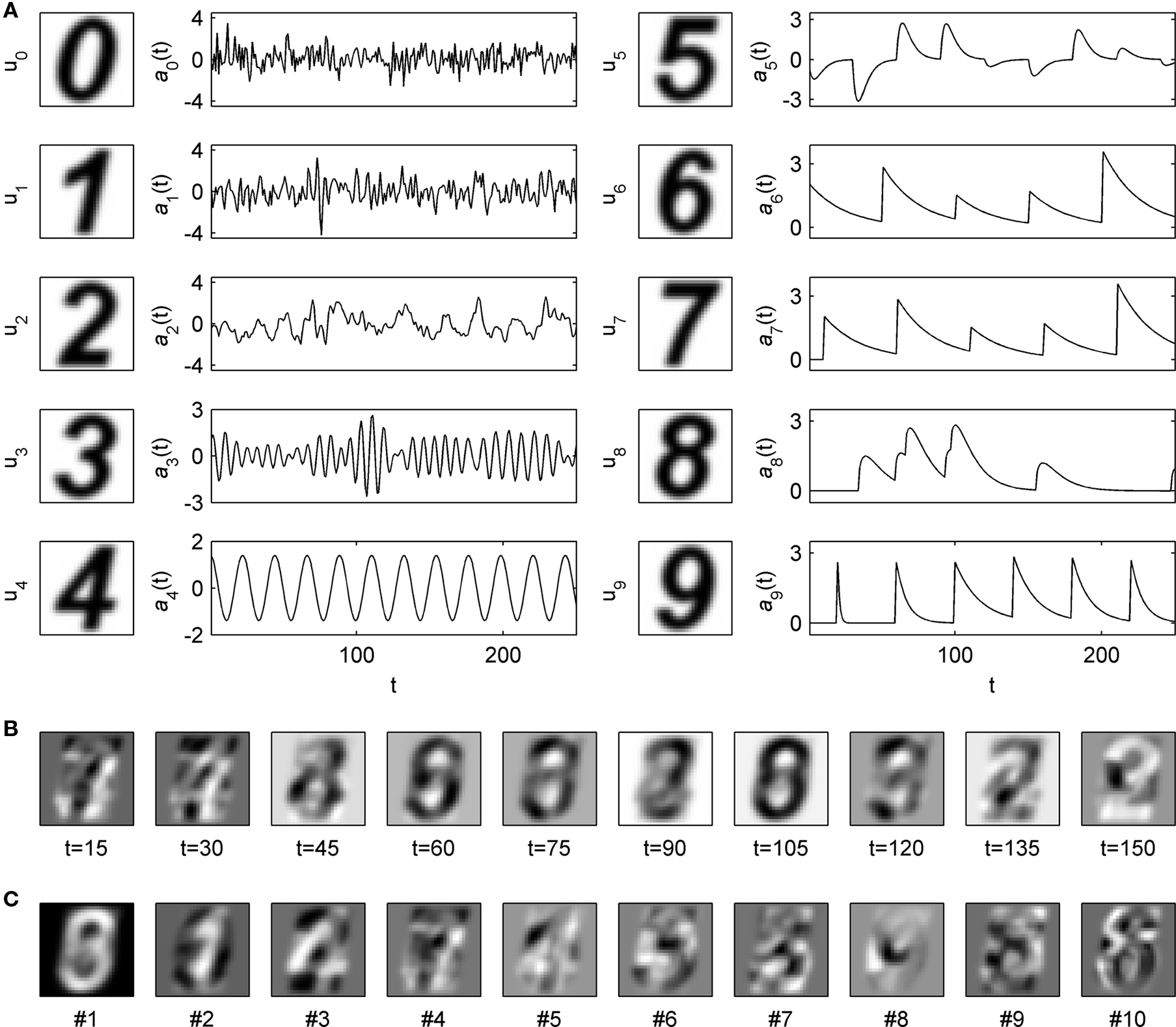
Figure 2. Construction of the artificial dataset. (A) construction of the data as a sum of 10 sources with fixed spatial components (left columns; u0,…,u9) and stochastic temporal components for which an exemplar realization of length T = 250 is shown (right columns; a0,…,a9). (B) Example of the observed data  for 10 values of t. The realizations of ai used in this example are those shown in (A). (C) Ten principal components obtained with standard PCA for the same data.
for 10 values of t. The realizations of ai used in this example are those shown in (A). (C) Ten principal components obtained with standard PCA for the same data.In Figure 3
A, we present an example of the results obtained by applying the algorithm to the artificial data. In this example, we used one realization of the data with length T = 1000. The objective function here was defined by taking γX = 1, γY = 0. We ran the algorithm 10 times on the same realization, using the 10 definitions of the signal and the noise. Figure 3
A shows  , i = 0,…9, the leading eigenvector obtained when the signal was defined as the i-th source. These eigenvectors are highly similar to the spatial component of the source defined as signal, i.e.,
  , and illustrate the success of the algorithm in recovering the signal’s spatial components in this particular case.
, i = 0,…9, the leading eigenvector obtained when the signal was defined as the i-th source. These eigenvectors are highly similar to the spatial component of the source defined as signal, i.e., , and illustrate the success of the algorithm in recovering the signal’s spatial components in this particular case.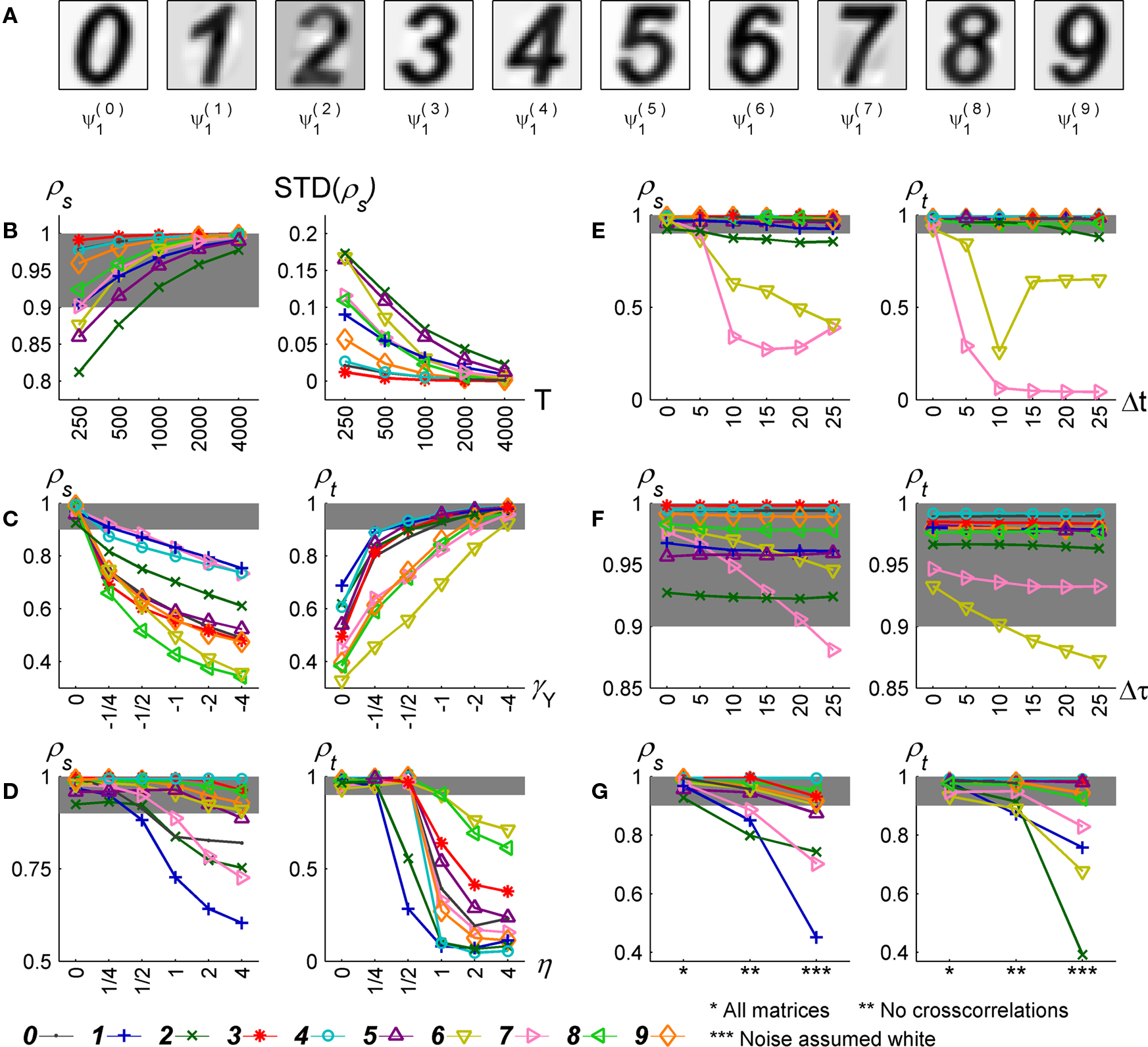
Figure 3. TSCA application on the artificial dataset. (A) Spatial components extracted by the algorithm from one realization of the data of length T = 1000. (B–G) Quantitative study of the performance of the TSCA algorithm. (B) Left – mean value of ρs, a measure of the quality of reconstruction of the spatial components, plotted against T. Right – standard deviation of ρs. (C) Left – mean value of ρs as a function of γY for γX = 1. Right – mean value of ρt, a measure of the quality of reconstruction of the temporal components, plotted as a function of γY. (D) Mean values of ρs (left) and ρt (right) as a function of η, the amplitude of perturbation of the correlation matrices used by the algorithm. (E) Mean values of ρs (left) and ρt (right) as a function of Δt, perturbation to simulation timing assumed when constructing correlation matrices involving processes 6 and 7. (F) Mean values of ρs (left) and ρt (right) as a function of Δτ, perturbation to decay time constant assumed when constructing correlation matrices involving processes 6 and 7. (G) Comparison of mean values of ρs (left) and ρt (right) in three cases: when the algorithm had access to all necessary correlation matrices (*), when crosscorrelation matrices were assumed null (**), and when noise was assumed white (***). In all panels, the shaded area corresponds to a performance measure higher than 0.9.
A more rigorous and quantitative study of the performance of the algorithm applied on the artificial data is presented in Figures 3
B–F. In Figure 3
B we studied the effect of the temporal length of the data T on the performance of the algorithm by running the algorithm as in Figure 3
A for 10000 realizations of Z and for several values of T. Similarity between  and the corresponding spatial component ui was quantified by
  equivalent here to the Pearson correlation coefficient due to normalization of the vectors; the subscript s is used here to indicate that the correlation is spatial. Figure 3
B (left) shows the values of ρs averaged over the 10000 realizations of Z, plotted against T for each of the 10 processes. As expected, increasing T improved the performance of the algorithm. For T ≥ 1000, all 10 processes had an average value of ρs greater than 0.9, but even for T = 250 the average ρs was greater than 0.9 for most process and greater than 0.8 for all processes. For a very large T, the average ρs approached 1. This result is in fact guaranteed by the mathematical formulation, and implies a near prefect match between
equivalent here to the Pearson correlation coefficient due to normalization of the vectors; the subscript s is used here to indicate that the correlation is spatial. Figure 3
B (left) shows the values of ρs averaged over the 10000 realizations of Z, plotted against T for each of the 10 processes. As expected, increasing T improved the performance of the algorithm. For T ≥ 1000, all 10 processes had an average value of ρs greater than 0.9, but even for T = 250 the average ρs was greater than 0.9 for most process and greater than 0.8 for all processes. For a very large T, the average ρs approached 1. This result is in fact guaranteed by the mathematical formulation, and implies a near prefect match between  and ui for every realization of Z. This behavior can be also seen in Figure 3
B (right), which shows that the standard deviation of ρs decays to zero as T increases. We further observed that the standard deviation of ρs was of the order of 1 − ρs. Since this behavior was found in all subsequent simulations, standard deviations are not shown in subsequent panels.
and ui for every realization of Z. This behavior can be also seen in Figure 3
B (right), which shows that the standard deviation of ρs decays to zero as T increases. We further observed that the standard deviation of ρs was of the order of 1 − ρs. Since this behavior was found in all subsequent simulations, standard deviations are not shown in subsequent panels.
and the corresponding spatial component ui was quantified by equivalent here to the Pearson correlation coefficient due to normalization of the vectors; the subscript s is used here to indicate that the correlation is spatial. Figure 3
B (left) shows the values of ρs averaged over the 10000 realizations of Z, plotted against T for each of the 10 processes. As expected, increasing T improved the performance of the algorithm. For T ≥ 1000, all 10 processes had an average value of ρs greater than 0.9, but even for T = 250 the average ρs was greater than 0.9 for most process and greater than 0.8 for all processes. For a very large T, the average ρs approached 1. This result is in fact guaranteed by the mathematical formulation, and implies a near prefect match between and ui for every realization of Z. This behavior can be also seen in Figure 3
B (right), which shows that the standard deviation of ρs decays to zero as T increases. We further observed that the standard deviation of ρs was of the order of 1 − ρs. Since this behavior was found in all subsequent simulations, standard deviations are not shown in subsequent panels.For further investigations we fixed T to the intermediate value of 1000 and repeated similar simulations while varying other parameters. In Figure 3
C we studied the effect of γX and γY on the performance. Since multiplying both γX and γY by a factor does not affect the resulting eigenvectors, we fixed γX = 1 and varied only γY. In Figure 3
C (left) we plotted the average value of ρs as a function of γY. Decreasing γY reduced ρs for all processes, albeit at different rates. However, there was an advantage to decreasing γY: the projection of the data on the first eigenvector  tended to be more correlated with the temporal component of the signal source ai. This behavior is quantified in Figure 3
C (right), where we plotted the average value of ρt, the Pearson correlation between
tended to be more correlated with the temporal component of the signal source ai. This behavior is quantified in Figure 3
C (right), where we plotted the average value of ρt, the Pearson correlation between  and ai, against γY; the subscript t is used here to indicate that the correlation is temporal. The average ρt increased when γY was decreased, and reached values close to 1 for γY = −4. Comparing the left and right panels of Figure 3
C, we observe that γY offers a tradeoff between the quality of spatial
and ai, against γY; the subscript t is used here to indicate that the correlation is temporal. The average ρt increased when γY was decreased, and reached values close to 1 for γY = −4. Comparing the left and right panels of Figure 3
C, we observe that γY offers a tradeoff between the quality of spatial  and temporal
  outputs of the algorithm. In general however, it is not guaranteed that ρt converges to 1 for large negative γY. This occurs only when there exist directions with non-zero signal power that are orthogonal to all directions with non-zero noise power. In this example one such direction indeed existed for each signal/noise definition: it was the direction in the 10 dimensional linear subspace spanned by all ui that was orthogonal to the 9 dimensional linear subspace spanned by the vectors ui designated as noise.
tended to be more correlated with the temporal component of the signal source ai. This behavior is quantified in Figure 3
C (right), where we plotted the average value of ρt, the Pearson correlation between and ai, against γY; the subscript t is used here to indicate that the correlation is temporal. The average ρt increased when γY was decreased, and reached values close to 1 for γY = −4. Comparing the left and right panels of Figure 3
C, we observe that γY offers a tradeoff between the quality of spatial and temporal outputs of the algorithm. In general however, it is not guaranteed that ρt converges to 1 for large negative γY. This occurs only when there exist directions with non-zero signal power that are orthogonal to all directions with non-zero noise power. In this example one such direction indeed existed for each signal/noise definition: it was the direction in the 10 dimensional linear subspace spanned by all ui that was orthogonal to the 9 dimensional linear subspace spanned by the vectors ui designated as noise.As discussed above, we view the requirement for knowing the correlation matrices to be the most restrictive assumption we make. In generating Figures 3
B,C we used the true correlation matrices, obtained from our knowledge of the generating processes. Clearly, parameters of the generating processes are unknown for real datasets, and the algorithm must use estimates of the correlation matrices. We used the artificial data to test the performance of the algorithm when provided with correlation matrices that were perturbed away from their true values. In view of the results in Figure 3
C, we quantified the algorithm’s performance using both ρs and ρt, with ρs evaluated for γX = 1, γY = 0, and ρt evaluated for γX = 1, γY = −4. In Figure 3
D we show the results of perturbing the correlation matrices by adding to them a random symmetric matrix with independent, zero-mean, normally-distributed entries. All correlation matrices were perturbed independently. The scaling of the perturbing matrix was determined such that the ratio between its Frobenius norm and the Frobenius norm of the correlation matrix was fixed to a predefined value η. In Figure 3
D (left) we show the average value of ρs for different values of η (the average was taken over realizations of the both the data and the perturbations). For most processes, ρs remained above 0.9 even when η was 4, i.e., when the amplitude of the perturbation was four times the amplitude of the true correlation matrices. For η ≤ 1/2 the perturbation had only a marginal effect for all processes. Performance in terms of ρt was somewhat less resistant to the perturbation, with a sharp decrease in ρt when the perturbation and the true correlation matrices had similar amplitudes (η = 1). Still, most processes were almost unaffected by perturbations with η ≤ 1/2.
Although the analysis in Figure 3
D validates the algorithm’s robustness with respect to random perturbations of the correlation matrices, the perturbation scheme we used might not capture the type of errors in estimated correlation matrices that are likely to occur in practical applications, as it is unlikely that these errors will be random. Thus, in Figure 3
E we studied another type of perturbation by replacing the true correlation matrices related to processes 6 and 7 with matrices calculated based on the true generating processes but with perturbed parameters. Specifically, the response onset times were delayed by Δt with respect to the true onset times. Marked reduction in performance was observed for perturbations of size greater than Δt = 5 time samples, which is 10% of the inter stimulus interval (50 time samples) and 20% of the exponential decay time constant (25 time samples). We note that the reduction in performance for large Δt was limited to process 6 and 7, even for Δt as high as 25. A different perturbation of the correlation matrices related to processes 6 and 7 is presented in Figure 3
F. Here, we manipulated the exponential decay time constant used in the calculation of the correlation matrices by increasing it by Δτ. In this case, performance for all processes was either unaffected or affected very moderately by the perturbation, even when the decay time constant was assumed twice its true value (Δτ = 25). Based on Figures 3
E,F, we conclude that the algorithm always showed some degree of robustness with respect to the perturbation of the generating process parameters, but with different sensitivity for different parameters. Similar behavior was observed for perturbation of the parameters of other processes (data not shown).
In Figure 3
G, we show that in some cases the algorithm can retain good performance even if some of the correlation matrices involved are completely unknown. Specifically, we tested the performance of the algorithm when (a) only the autocorrelation matrices but not the cross correlation matrices were assumed to be known and (b) when only the signal’s autocorrelation matrix was known and the noise was assumed to be white. These two approaches can be viewed as the result of heuristically replacing unknown auto- and cross-correlation matrices with generic matrices, i.e., the identity and zero matrices, respectively. Omission of the cross correlation matrices led to a decrease in performance that was limited to the two pairs of coupled processes (1,2 and 6,7). Still, both ρs and ρt reached reasonable values of 0.8 or higher for these processes. The white noise approach led to a more pronounced decrease in performance. However, this reduction was again limited mainly to the coupled processes, with an only moderate decrease in performance for the other processes. This result suggests that the white noise approach, which reduces significantly the number of correlation matrices that have to be known or estimated, can be useful for certain datasets. The fact that the algorithm performed well for most processes despite the strong deviation between the true and putative correlation matrices is a further indication of the algorithm’s robustness.
We presented an algorithm for the analysis of temporally structured multidimensional data. Our approach in designing the algorithm was to allow it to benefit as much as possible from prior knowledge about the temporal structure of the data. We proposed a framework in which this knowledge can be expressed mathematically, and an algorithm for using it to extract spatial structures and finer temporal details from the data.
A principal feature of the algorithm is the characterization of the temporal structure of the underlying sources through correlation matrices. This approach allows the algorithm to deal with a very broad class of signal and noise sources. Specifically, we have shown that if the necessary correlation matrices are known, the algorithm is applicable whenever the following assumptions hold: (1) the signal and the noise combine additively; (2) the “contrastability” condition is satisfied, which, loosely speaking, means that the signal and the noise are sufficiently different; and (3) there is sufficient amount of data. Thus, common assumptions such as independence of the signal and noise or stationarity are not required (these cases are respectively dealt with by the appropriate interaction correlation matrices and non-Toeplitz correlation matrices); the algorithm can in principle be applied to arbitrarily complex signal or noise sources. Still, this versatility critically depends on the knowledge of the necessary correlation matrices. Below we demonstrate how prior temporal knowledge can be used to construct the correlation matrices for several prototypical types of sources.
Processes 5–8 in Figures 2 and 3
represent a specific type of stimulus-triggered response, where the temporal structure of the response is equal for all channels, up to scaling. Equivalently, a response of this type can be described as the synchronous emergence over all channels of a particular spatial pattern, i.e., an “activation map”. We can consider a general form for such a signal, [X]pt = Σlςprlg(t − tl), with p and t denoting respectively channel and time indices, ςp denoting the scaling of channel p, tl denoting the time of stimulation l, g(·) being the temporal profile of the response, and rl being independent and identically distributed random variables representing the amplitudes of the responses. When calculating the necessary correlations matrices we find that there is a single correlation matrix associated with sources of this class; this correlation matrix is given by
where cv is the coefficient of variation of any of the variables rl, and δ is Kronecker’s delta. Thus, the temporal information required for constructing the correlation matrix is the time of stimulation, the coefficient of variation of the response amplitude, and the temporal profile of the activation, which has to be known only up to scaling. In practical applications, these quantities are either known or can be estimated: the time of stimulation is known as it is set by the experimental protocol; the activation function can be estimated based on a preliminary analysis or on some canonical form (as it is commonly done for fMRI data, where the activation function is the hemodynamic response function); and the coefficient of variation, which measures the regularity of the response, can be estimated based on a preliminary analysis or on theoretical grounds.
Another class of sources is represented by processes 0–4. These sources are stationary fluctuations of a fixed spatial pattern; the amplitude of these fluctuations is determined by a zero-mean stationary process a(t) : [X]pt = ςpa(t). In this case, the single correlation matrix associated with the process is a Toeplitz matrix whose value at row t and column t′ is given by the value of the autocovariance sequence of a(t) at lag t − t′. In turn, the autocovariance sequence can be expressed as the Fourier transform of the power spectrum of the process a(t), a quantity denote by S(f), with f being the frequency in radians per sample. The correlation matrix can thus be expressed as:  (this particular form of the Fourier transform was chosen because t takes discrete values). In order to construct the correlation matrix for stationary sources of this type it is therefore sufficient to have an estimate of the power spectrum of the fluctuations, up to scaling. We suggest that such estimation is possible in some cases. For example, approximately periodic processes, such as those related to heartbeat or respiration, have highly concentrated spectra with most energy concentrated around a fundamental frequency and possibly around higher order harmonics. Estimation of the spectrum in this case reduces to the estimation of the fundamental frequency, and the relative contribution of different harmonics. We also note that in the case where the signal’s spectrum is assumed to take a constant value within a narrow band around a particular frequency, there is an interesting relation to the theory of multitaper spectral estimation (Thomson, 1982
; Percival and Walden, 1993
). The estimator mQ(ψ) can be then viewed as a weighted sum of an estimator for the signal power and an estimator for the noise power, where the signal estimator is a multitaper spectral estimator constructed with all Slepian tapers scaled by their eigenvalues.
(this particular form of the Fourier transform was chosen because t takes discrete values). In order to construct the correlation matrix for stationary sources of this type it is therefore sufficient to have an estimate of the power spectrum of the fluctuations, up to scaling. We suggest that such estimation is possible in some cases. For example, approximately periodic processes, such as those related to heartbeat or respiration, have highly concentrated spectra with most energy concentrated around a fundamental frequency and possibly around higher order harmonics. Estimation of the spectrum in this case reduces to the estimation of the fundamental frequency, and the relative contribution of different harmonics. We also note that in the case where the signal’s spectrum is assumed to take a constant value within a narrow band around a particular frequency, there is an interesting relation to the theory of multitaper spectral estimation (Thomson, 1982
; Percival and Walden, 1993
). The estimator mQ(ψ) can be then viewed as a weighted sum of an estimator for the signal power and an estimator for the noise power, where the signal estimator is a multitaper spectral estimator constructed with all Slepian tapers scaled by their eigenvalues.As a final example of processes that can be dealt with by the algorithm we consider a simple traveling wave of the form [X]pt = sin (Kp − ft − ϕ), where K is the spatial frequency, p is the channel index that corresponds in this case to some location on a line, f is the temporal frequency, and ϕ is the random phase. This example is qualitatively different from the previous examples because a traveling wave cannot be described as fluctuations of a fixed spatial pattern, and therefore it cannot be dealt with by the simplified algorithm. Calculating the correlation matrices, we find that depending on the distribution of ϕ, either a single correlation matrix is required, [C]tt′ = cos(f(t − t′)), or three correlation matrices are required, [C1]tt′ = cos(f(t − t′)), [C2]tt′ = cos(f(t + t′)), and [C3]tt′ = sin(f(t + t′)) (the latter case occurs whenever E(e2iϕ) ≠ 0). In this case, all the information required to construct the correlation matrices is the wave’s temporal frequency, and a specific characteristic of the distribution of the phase.
Though different, the three examples of source types given above illustrate a common scheme that can be used to construct the correlation matrices in practical applications. First, theoretical correlation matrices are calculated based on an idealized generative process or a “toy model” for a source, e.g., the equation for the synchronized stimulus-triggered response given above. Then, the actual matrices are calculated, either by estimating the remaining free parameters of the correlation matrices, e.g., the shape of the response function, or simply by plugging in known values for these parameters, e.g., stimulation times. What limits the method in this respect is thus the ability to postulate appropriate generative equations for the model, calculate the theoretical correlation matrices, and estimate the free parameters.
Regardless of the exact way by which the correlation matrices are constructed, they can be viewed as “weak models” of the data in the sense that they describe its structure not by specifying a full probability density function but only through its second order moments. The method can be therefore placed somewhere between parametric and non-parametric methods. Non-parametric methods such as PCA incorporate the assumption that the temporal structure of the data is unknown. Other methods such as independent component analysis (ICA; e.g., Hyvärinen and Oja, 2000
) usually make very weak assumptions about the temporal structure of the data, e.g., that the signal and noise are statistically independent. These methods can be highly useful in many cases and offer the best solution one can hope for in situations where indeed temporal information is unavailable. However, many times this is not the case. Information about the frequencies of different signals or about points in time where they emerge is often at hand. Moreover, some of the temporal aspects of the data are in fact defined by the experimental protocol, and therefore can be controlled by the experimentalist, e.g., by setting the stimulation frequency. On the other hand, parametric methods such as Bayesian methods make the opposite extreme assumption, by requiring a complete statistical description of the data. Under such strong assumptions, Bayesian methods are optimal. In practice, the true probability function generating the data is rarely known and may be very difficult to estimate. This limits the applicability of parametric methods in many neuroscience contexts.
The present method offers a compromise between these two approaches. In this respect, it is similar in spirit to the common practice of filtering the data at a specific frequency band or applying other Fourier-theoretical tools. In these cases, frequency-domain information is used without an explicit specification of a full probability function. However, such procedures assume stationarity, at least locally, and ignore any information about the signal’s temporal phase. In addition, Fourier based methods are often applied independently for each channel, and therefore ignore the multidimensionality of the data. One spectral method that is inherently multidimensional is “space frequency SVD” (Mitra and Pesaran, 1999
). The mathematical formulation of this method, which involves multitaper spectral estimators, is somewhat similar to the formulation presented above for the application of the algorithm on stationary data. However, whereas space frequency SVD assumes the different signals to be stationary, with well-localized non-overlapping spectra, our approach relaxes these assumptions and is therefore applicable to a wider class of problems.
The idea of exploiting temporal structures in the data has been incorporated into both PCA and ICA frameworks before (Molgedey and Schuster, 1994
; Ziehe and Müller, 1998
; Sornborger et al., 2005
; de Cheveigné and Simon, 2007
), albeit for more specific setups. Out of these algorithms, we find constrained ICA (cICA; Lu and Rajapakse, 2000
, 2005
; James and Gibson, 2003
) to be most similar to TSCA in several aspects. The cICA algorithm finds independent components in the data that satisfy user-defined temporal constraints. This algorithm thus elegantly incorporates prior knowledge about the temporal structure of the data into the analysis procedure, and is similar in this respect to our algorithm. There are, however, several fundamental differences between our algorithm and the family of ICA methods, and in particular cICA. Specifically, our algorithm does not require the data to be a mixture of a finite number of statistically-independent signals, which is the basic ICA assumption. This assumption is restrictive in many practical cases, because it doesn’t allow any correlations between the signal and the noise. Moreover, for signals such as the traveling wave considered above, no ICA decomposition is feasible. In contrast, our algorithm readily deals with statistical dependencies in the data, as demonstrated by Figures 2 and 3
. Another difference between ICA and our algorithm is that ICA typically requires the number of components constituting the data to be known a-priori, whereas TSCA is more flexible as this number is not explicitly required. Rather, the number of signal autocorrelation matrices supplied to the algorithm serves only as a lower bound for the number of signal components. An additional difference between ICA algorithms and TSCA is that ICA typically allows only one component to be Gaussian. No such restriction is imposed in our case. This is demonstrated in Figures 2 and 3
, in which processes 0–4 are Gaussian.
The cICA algorithm, while in rationale very similar to our algorithm, uses a mathematical construction very different from ours. In particular, our objective function is quadratic, so its maximization requires the solution of a linear system, given by a matrix diagonalization problem. Standard linear algebra methods are applicable and, unlike cICA, a search for locally optimal solutions is not necessary. An additional difference is that TSCA not only takes into account the temporal structure of the signal, through the signal correlation matrices, but also that of the noise, through the noise correlation matrices. More importantly, although cICA is defined using a very general theoretical framework that allows for a wide range of temporal constraints, practical applications of cICA and the development of stable numerical schemes for solving the cICA problem have been mainly restricted to constraining the time course of the components to be correlated with an a-priori known reference signal. The reference signal, whether derived from an independent measurement, a preliminary analysis, or theoretical considerations, requires the knowledge of the approximate behavior of the time course on a single trial basis. Thus, reference cICA addresses only a subclass of problems that are addressable with TSCA, which requires only knowledge of long term second order statistics.
While parallels between ICA methods and our algorithm can be drawn, we find TSCA to be most similar to PCA, as our objective function is a direct generalization of the PCA objective function. The utility of PCA for data of the type we considered here is often questioned on the merit that it produces non-interpretable components. We endorse this observation, but point out that the typical failure of PCA stems not from the uselessness of the PCA strategy, i.e., the extraction of components with high power, but from the fact that it fails to distinguish between components of interest (signal) and nuisance components (noise). Our algorithm tackles this problem directly, and while maintaining the basic PCA principles, uses an objective function that contrasts the signal to the noise. To estimate the objective function we take into account the temporal structure of the data, which is ignored in naïve PCA applications. The output of the algorithm, is analogous to the PCA output, and is given by spatial components ranked by their score on the objective function and associated with temporal projections. PCA itself is often described as a rotation of the (spatial) coordinates followed by a projection on the leading coordinates. The same description holds here. The main difference is that the rotation performed here yields projections that have some prescribed temporal properties. Finally, there is an even stronger relation between PCA and TSCA for the particular choice of an objective function with γX = 1, γY = 0. As it follows from the analysis in Section 1 of the Supplementary Material, the operation of TSCA in this case is nothing but PCA performed on the signal alone, with the noise completely ignored.
From a computational perspective, the difference between PCA and the present algorithm amounts to the diagonalization of a matrix of the form ZQZT instead of ZZT. A related difference is that the objective function used here is not necessarily positive; correspondingly, neither Q nor ZQZT are necessarily positive semi definite. As a result, the eigenvalues of ZQZT can be either positive or negative. Throughout the paper we have focused on components with the largest eigenvalues, which estimate leading components of the signal. However, components with highly negative eigenvalues can be of interest as well in some cases. Consider for example the case where the signal and the noise are spatially orthogonal, i.e., all directions with positive signal power are orthogonal to all directions with positive noise power. If an objective functions with γX = 1, γY < 0 is selected, the trailing TSCA components, which achieve highly negative scores on the objective function, are the dominant components of the noise, regardless of the precise value of γY. In more realistic cases, where the signal and noise are only approximately spatially orthogonal, we can still expect trailing components to exhibit some resemblance to dominant noise components. This can be seen in Figure 1
D, where the spatial components of the signal and noise are approximately orthogonal  and the trailing TSCA eigenvector ψ2 is similar to the noise spatial component uY. In Figure 1
E, where the roles of the signal and noise are switched, ψ2 resembles uX. This observation gives rise to an interesting interpretation of TSCA for cases where the signal and noise are approximately orthogonal. The algorithm can be viewed as splitting the data space into two orthogonal subspaces. One space, spanned by the leading eigenvectors with positive eigenvalues, corresponds to the signal, while the other one, spanned by the trailing eigenvectors with negative eigenvalues, corresponds to the noise. We note that the dimensionality of these subspaces is related to the eigenspectrum of Q: by Sylvester’s law of inertia (Ostrowski, 1960
) the number of positive (or negative) eigenvalues of Q sets an upper bound for the dimension of the signal (or noise) subspace.
and the trailing TSCA eigenvector ψ2 is similar to the noise spatial component uY. In Figure 1
E, where the roles of the signal and noise are switched, ψ2 resembles uX. This observation gives rise to an interesting interpretation of TSCA for cases where the signal and noise are approximately orthogonal. The algorithm can be viewed as splitting the data space into two orthogonal subspaces. One space, spanned by the leading eigenvectors with positive eigenvalues, corresponds to the signal, while the other one, spanned by the trailing eigenvectors with negative eigenvalues, corresponds to the noise. We note that the dimensionality of these subspaces is related to the eigenspectrum of Q: by Sylvester’s law of inertia (Ostrowski, 1960
) the number of positive (or negative) eigenvalues of Q sets an upper bound for the dimension of the signal (or noise) subspace.More generally, the algorithm puts forward a unified framework by which many types of signals can be characterized and studied in a systematic manner. Because of its generality and versatility, we propose that this method can be highly useful for exploratory analysis. In an exploratory context the construction of the weak models, i.e., the estimation of the correlation matrices, can be based on hypotheses rather than on well-established knowledge. In other words, if one can make a good guess about the temporal structure of the data and formulate it through appropriate correlation matrices, the algorithm can be applied to find both spatial components and a more detailed temporal structure. Our studies show that the algorithm always displays at least some degree of robustness to perturbations of the correlation matrices (Figure 3
). Thus, the algorithm exhibits some tolerance to errors in the hypotheses under which the correlation matrices are constructed. This robustness suggests an interesting possibility of learning the correlation matrices from the data, through an iterative scheme. Such an adaptive algorithm can be highly beneficial, as it might make use of even more limited knowledge about the temporal structure of the data. However, transforming this idea into a rigorous algorithm is beyond the scope of the current contribution and it is left for future research.
The author declares that the research was conducted in the absence of any commercial or financial relationships that could be construed as a potential conflict of interest.
I deeply thank Misha Tsodyks for ongoing assistance and support, Omri Barak for valuable discussions and critical reading of the manuscript, and an anonymous reviewer for numerous helpful suggestions. I also thank Alex Loebel, Son Preminger and Alik Mokeichev for critical reading of the manuscript in various stages of its preparation.
The Supplementary Material for this article can be found online at http://www.frontiersin.org/computationalneuroscience/paper/10.3389/neuro.10/028.2009/
- ^ A closely related method is singular value decomposition (SVD); PCA is commonly solved by performing SVD on the data, typically after its mean was subtracted as preprocessing step. In the analysis presented here, we do not subtract explicitly the mean, so our discussion is applicable to SVD as well as PCA. For consistency with standard formulations of PCA, one can assume that the data is already centered.