Asteroseismic Signature of a Large Active Region
 Emanuele Papini
 Laurent Gizon
- 1Max-Planck-Institut für Sonnensystemforschung, Göttingen, Germany
- 2Institut für Astrophysik, Georg-August-Universität Göttingen, Göttingen, Germany
Axisymmetric magnetic activity on the Sun and sun-like stars increases the frequencies of the modes of acoustic oscillation. However, it is unclear how a corotating patch of activity affects the oscillations, since such a perturbation is unsteady in the frame of the observer. In this paper we qualitatively describe the asteroseismic signature of a large active region in the power spectrum of the dipole (ℓ = 1) and quadrupole (ℓ = 2) p modes. First we calculate the frequencies and the relative amplitudes of the azimuthal modes of oscillation in a frame that corotates with the active region, using first-order perturbation theory. For the sake of simplicity, the influence of the active region is approximated by a near-surface increase in sound speed. In the corotating frame the perturbations due to (differential) rotation and the active region completely lift the (2ℓ + 1)-fold azimuthal degeneracy of the frequency spectrum of modes with harmonic degree ℓ. Then we transform to an inertial frame to obtain the observed power spectrum. In the frame of the observer, the unsteady nature of the perturbation leads to the appearance of (2ℓ + 1)2 peaks in the power spectrum of a multiplet. These peaks blend into each other to form asymmetric line profiles. In the limit of a small active region (angular diameter less than 30°), we approximate the power spectrum of a multiplet in terms of 2 × (2ℓ + 1) peaks, whose amplitudes and frequencies depend on the latitude of the active region and the inclination angle of the star's rotation axis. In order to check the results and to explore the non-linear regime, we perform numerical simulations using the 3D time-domain pseudo-spectral linear pulsation code GLASS. For small sound-speed perturbations, we find a good agreement between the simulations and linear theory. Larger perturbation amplitudes will induce mode mixing and lead to additional complex changes in the predicted power spectrum. However linear perturbation theory provides useful guidance to search for the observational signature of large individual active regions in stellar oscillation power spectra.
1. Introduction
Surface magnetic activity shifts the frequencies of the global modes of acoustic oscillation during solar and stellar activity cycles (e.g., Pallé et al., 1989; García et al., 2010; Santos et al., 2016; Kiefer et al., 2017). Asteroseismology can in turn inform us about the strength and the latitude distribution of a band of magnetic activity on the stellar surface (Gizon, 2002; Chaplin et al., 2007; Gizon et al., 2016). However, the signature of a single large active region in stellar p-mode oscillation power spectra has not been discussed so far in detail. A complication inherent to this problem comes from the fact that the perturbation associated with a rotating active region is not steady in the observer's frame. Yet, this problem is relevant, since large starspots are detected in photometric variability (e.g., Mosser et al., 2009) and using Doppler or Zeeman-Doppler imaging (e.g., Strassmeier, 2009).
We build on preliminary work by Gizon (1995, 1998) who considered the effect of a single sunspot in corotation on the low-degree modes of solar oscillation. The problem of unsteady perturbations has been considered in the past in different contexts. The interaction with acoustic modes with an inclined magnetic field with respect to the stellar rotation axis was first studied by Kurtz (1982) to explain the oscillation power spectra of roAp stars (see also Kurtz, 2008). In the oblique pulsator model the effect of the magnetic field dominates over rotation, and the pulsation axis is aligned with the magnetic axis of the star. Only modes of oscillations symmetric with respect to the magnetic field axis are excited. The oblique pulsator model was extended by Dziembowski and Goode (1985) to include the first-order effects of the Coriolis and Lorentz forces, and then by Shibahashi and Takata (1993) to account for the distortion in the eigenfunctions. In parallel Dziembowski and Goode (1984) and Gough and Taylor (1984) discussed the combined influence of rotation and of an inclined magnetic field in corotation on multiplets of solar acoustic oscillations. They explicitly mentioned that each multiplet consist of (2ℓ + 1)2 components in the power spectrum (this was already hinted at by Dicke, 1982).
We focus on stars with a level of activity higher than the Sun, which may have active regions with larger surface coverage, and therefore better chances for detection. Following the same approach of Goode and Thompson (1992), we investigate the linear changes induced in a nℓ-multiplet by an unsteady perturbation that mimics an active region (AR) rotating with the star. In particular we study the power spectra of the dipole and quadrupole multiplets. For the active region we consider a simple two-parameter model, where near-surface sound-speed perturbations have a given amplitude and surface coverage.
As a complement to the linear analysis we also explore the non-linear regime of the active-region perturbation by means of 3D numerical simulations, by studying the combined effect of rotation and mode mixing on the observed power spectra using the wave propagation code GLASS (see Hanasoge and Duvall, 2007; Papini et al., 2015). We note that the non-linear regime was studied in the context of strong magnetic fields in roAp stars by, e.g., Cunha and Gough (2000); Bigot and Dziembowski (2002); Saio and Gautschy (2004), and Cunha (2006).
2. Methods
2.1. Signature of an Active Region in the Oscillation Power Spectrum: Linear Theory
2.1.1. Linear Problem in the Corotating Frame
The normal modes of oscillation of a spherically symmetric non-rotating star are identified by three integer numbers: the radial order n, the angular degree ℓ, and the azimuthal order m, with |m| ≤ ℓ. In the absence of attenuation the degenerate mode frequencies, , are real and the displacement eigenvectors solve the linearized equation of motion
where is a linear spatial differential operator (see e.g., Unno et al., 1989). Hereafter superscripts “(0)” denote quantities associated with the non-rotating stellar model. In spherical polar coordinates r = (r, θ, ϕ), the displacement eigenfunctions can be written as
where are spherical harmonics and ξr, nℓ and ξh, nℓ are functions of radius only that can be calculated numerically for a given stellar model (see e.g., Aerts et al., 2010).
We now consider two perturbations, the first perturbation due to rotation (e.g., Hansen et al., 1977) and the second arising from the presence of an active region that rotates with the star (see e.g., Schunker et al., 2013, for the effect of a sunspot on high-degree modes). The latter perturbation is unsteady in an inertial frame of reference. Here we aim to study how these two effects may affect the fine structure of the modes within a fixed multiplet (n, ℓ). The two perturbations taken together completely remove the (2ℓ + 1)-fold degeneracy in m.
Provided that there is only one active region, it is much more convenient to first tackle the problem in a reference frame that is corotating with the active region, where both perturbations are steady (e.g., Dziembowski and Goode, 1984; Goode and Thompson, 1992). In Figure 1 we define three frames of reference, , , and , all three with the same origin at the center of the star. Frame is an inertial frame of reference, with polar axis z pointing toward the observer. We denote by β the colatitude of the active region in frame . The other two frames are both corotating with the active region at the angular velocity Ωβ about the rotation axis of the star. The polar axis of is directed along the stellar rotation axis and is inclined by an angle i with respect to z. The polar axis of the frame is inclined by the angle β with respect to the rotation axis. In the center of the active region is at the north pole. Provided that the starspot has no proper motion, the angular velocity Ωβ is equal to the surface rotational angular velocity of the star at colatitude β. We call r = (r, θ, ϕ), rβ = (r, θβ, ϕβ), and the spherical-polar coordinates associated with , , and , respectively.
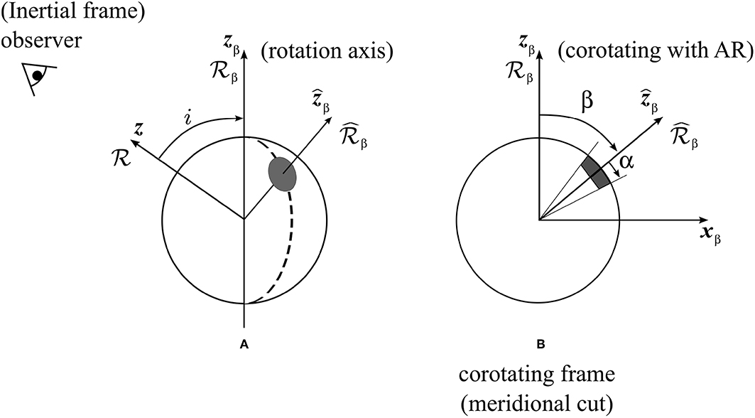
Figure 1. Reference frames and angles of the problem. Arrows show the polar axes of the coordinate systems , , and . The frame is the inertial frame of the observer. The rotation axis of the star is inclined by an angle i with respect to the line of sight. Both frames and corotate with the active region (shaded area) at a constant angular velocity Ωβ. The polar axis of is aligned with the rotation axis of the star. In the active region has a colatitude β and in it is at the pole.
We consider the effects of rotation and the active region on the acoustic oscillations as small perturbations. In the frame each mode is identified by the index M, −ℓ ≤ M ≤ ℓ, and we expand the displacement eigenvectors and eigenfunctions as
and
where δξnℓM is orthogonal to each unperturbed eigenvector with the same ℓ and n (e.g., Gough and Thompson, 1990), and the coefficients are (real) amplitudes. We write the wave operator as
with
where accounts for the effects of rotation and for the effects of the active region.
To first order, the linearized equation of motion reduces to
We define the inner product between two vectors ξ(rβ) and η(rβ) on the Hilbert space of displacement vectors as
where * denotes the complex conjugate and V is the stellar volume. The unpertubed eigenmodes are normalized such that
We take the inner product of Equation (7) with to obtain
Because is Hermitian symmetric and , the second term on the left-hand side of the above equation vanishes
Introducing the perturbation matrix elements
where
Equation (9) becomes
To simplify the notation we dropped the indices nℓ on δωM. In matrix form,
where is the vector of amplitudes. To find AM and δωM we have to solve the above eigenvalue problem, Equation (14).
The rotation perturbation matrix OΩ is diagonal in the frame . The active region perturbation matrix OAR is not diagonal in , but it can be obtained in terms of the diagonal perturbation matrix expressed in the frame ,
where the matrix R(ℓ) performs a clockwise rotation of β about the y axis that transforms the frame into the frame . More explicitly, the elements of the rotation matrix are given by
where is given by Messiah (1960).
2.1.2. Frequency Splittings Due to Rotation
In the corotating frame the rotation perturbation matrix is diagonal:
with
where Ω(r, θ) is the internal angular velocity in an inertial frame. By construction, the angular velocity Ωβ of the frame is Ωβ = Ω(R, β), where R is the radius of the star. The first and second terms on the right-hand side of Equation (18) describe the effect of differential rotation, where the functions Knℓm(r, θ) are the rotational sensitivity kernels (Hansen et al., 1977) and Cnℓ are the Ledoux constants (Ledoux, 1951) that account for the effect of the Coriolis force. The last term describes the quadrupole distortion of the star due to the centrifugal forces (e.g., Saio, 1981; Aerts et al., 2010) and is proportional to the ratio of the centrifugal to the gravitational forces at the surface η = Ω2R3/(GM), where M is the mass of the star and G is the universal constant of gravity. The term Q2ℓm accounts for the quadrupolar component of the centrifugal distorsion
where are the associated Legendre functions and P2 is the Legendre polynomial of second order. The centrifugal term is very small in the case of slow rotators like the Sun (Dziembowski and Goode, 1992), however it increases rapidly with rotation and it is not negligible anymore for stars rotating a few times faster than the Sun (e.g., Gizon and Solanki, 2004).
2.1.3. Frequency Splittings Due to the Active Region
In this section we parametrize the effects of the active region on the oscillation frequencies in the corotating frame , where the active region is at the north pole.
Modeling the complex influence of surface magnetic fields on acoustic oscillations is challenging (e.g., Gizon et al., 2010; Schunker et al., 2013). Here we choose to drastically simplify the physics and to focus on the geometrical aspects of the problem.
Assuming that the area of the active region covers a polar cap with (see Figure 1) and that the structure of the active region is separable in r and , we can parametrize the perturbation matrix as follows:
where
is a geometrical weight factor that accounts for the surface coverage of the active region. For small values of α, decreases fast as |m″| increases (Figure 2). Since the value of does not depend on the sign of m″, the eigenvalues of OAR are degenerate in |m| (see also, e.g., Kurtz and Shibahashi, 1986).
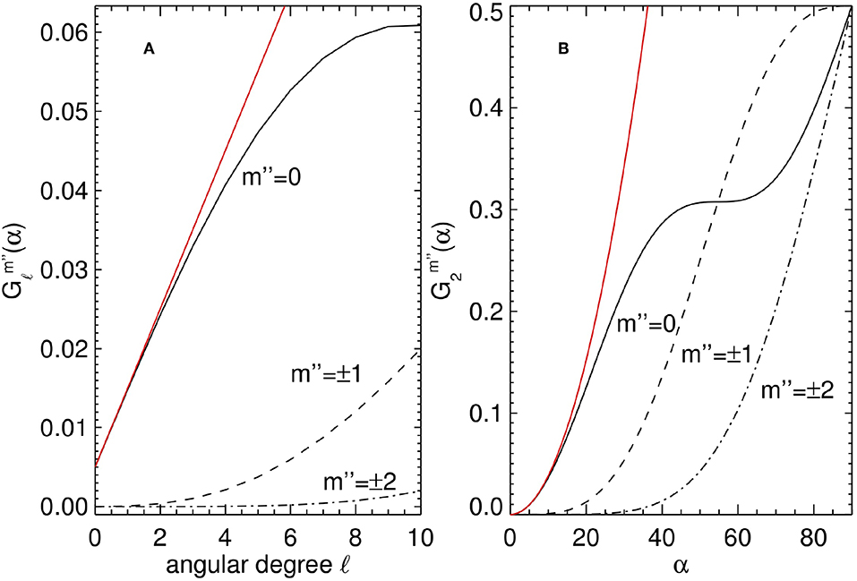
Figure 2. (A) Geometrical weight factor defined by Equation (21) as a function of angular degree ℓ for m = 0, ±1, ±2, at fixed α = 8°. (B) as a function of α for ℓ = 2. The red curves show the parabolic approximations for in the limit of small α (see section 3.2.3, Equation 59).
The parameter εnℓ is a measure of the relative magnitude of the active region perturbation and contains all the physics. From studies of local helioseismology (e.g., Gizon et al., 2009; Moradi et al., 2010; Schunker et al., 2013), it is known that the net effect of an active region is to increase the frequencies of acoustic modes, i.e., waves propagate faster in magnetic regions and thus εnℓ is positive. Since the active region introduces a perturbation that is strongly localized near the surface, the value of εnℓ increases with radial order n. A proper calculation of the value of εnℓ goes beyond the scope of the present study. Instead, we parametrize the active region perturbation as an increase in sound speed near the surface. Following Papini et al. (2015), we write
where ρ0(r) is the density of the unperturbed stellar background and Δc2(r) is the radial change in the squared sound speed. Here the integral is over the radial extent of the active region. In section 2.2 we will further specify the effective sound-speed perturbation.
Using Equation (15), the perturbation matrix elements in frame are
We note that for ℓ ≤ 3 and α ≲ 30°, we have , where |m″| ≠ 0, and therefore the dominant eigenvalue is , see Equation (20).
2.2. Numerical Setup for the Linear Problem
We now introduce the internal rotation model and the active region parameters, used to illustrate the theory. We consider a star with a rotation period of 8 days, about one third the rotation period of the Sun. This choice of rotation period ensures that the azimuthal modes in a multiplet are well separated in frequency space. For the internal rotation profile, we take
which is a scaled model of solar differential rotation as in Gizon and Solanki (2004). The centrifugal term has a significant effect. It shifts the m = 0 mode and introduces an asymmetry in the shifts for positive and negative azimuthal orders m, with a maximum frequency shift of more than 100 nHz in the case of a multiplet near 3 mHz. Therefore this term must be included when performing the analysis.
From observations of p-mode frequency changes during the solar cycle, Libbrecht and Woodard (1990) showed that the (positive) frequency shifts are almost independent of ℓ and increase with frequency, thus indicating that the effects of magnetic activity on acoustic oscillations are confined to the surface. Assuming that the perturbation covers two pressure scale heights below the photosphere and setting Δc2/c2 ≃ 10% there, Equation (22) gives εnℓ ≃ 0.003 at frequencies near 3 mHz. The surface coverage of a stellar active region, as inferred from Doppler imaging, ranges from a percent up to 10% (Strassmeier, 2009). Here we consider two different surface coverages of either 4% or 7%, corresponding to cosα = 0.92 or 0.86 (α ≃ 23° or 30°). Finally, we consider an active region at a colatitude of either β = 20° (near the pole) or 80° (near the equator).
In the following section we focus on two multiplets with (ℓ, n) = (1, 18) and (2, 18). For each of these modes we solve the eigenvalue problem (14) by means of Jacobi's method (Press et al., 1992). For the calculation of the unperturbed eigenmodes we use the ADIPLS software package (Christensen-Dalsgaard, 2008) and solar Model S as the reference structure model (Christensen-Dalsgaard et al., 1996). The unperturbed frequencies of the dipole and quadrupole modes are 2695.40 and 2756.95 μHz, respectively. We note that the choice of reference solar model is unimportant for the present study.
2.3. Power Spectrum in the Observer's Frame: (2ℓ + 1)2 Peaks
Given particular values for α, β, and εnℓ the eigenvalue problem (14) is fully specified and can be solved. In this section we use the solutions (3) and (4) to build a synthetic power spectrum in the observer's frame, in order to relate the results to observations.
We need to find an expression that connects the eigenmodes to the observed intensity fluctuations. For the sake of simplicity, we assume that the variation I(θβ, ϕβ, t) induced by the acoustic oscillations in the emergent photospheric intensity is proportional to the Eulerian pressure perturbation p of the acoustic wavefield (e.g., Toutain and Gouttebroze, 1993), as measured at the stellar surface r = R. The pressure perturbation p is related to the wavefield displacement ξ through the linearized adiabatic equation
where c0 and P0 are, respectively, the sound speed and the pressure of the unperturbed stellar model. The pressure perturbation pnℓM(r, θβ, ϕβ) of the mode M is
where ξnℓM is given by Equation (3). To leading order, we have
with
where we dropped the subscripts nℓ. Acoustic oscillations in stars are stochastically excited and damped by turbulent convection, therefore I(θβ, ϕβ, t) is a realization of a random process. Since the perturbation is steady in the frame , this random process is stationary in that frame. An expression for the intensity fluctuations I(θβ, ϕβ, ω) in Fourier space with the required statistical properties is
where the are independent complex Gaussian random variables, with zero mean and unit variance:
In Equations (27) and (28) we only consider the positive-frequency part of the spectrum (ω and ω′ > 0) since I(θβ, ϕβ, t) is real. The negative-frequency part is related to the positive part by . The function LM(ω) is a Lorentzian
appropriate for describing the power spectrum of an exponentially damped oscillator with full width at half maximum (FWHM) Γ (see e.g., Anderson et al., 1990).
We transform Equation (27) back to the time domain by inverse Fourier transformation to obtain I(θβ, ϕβ, t). The intensity I(θ, ϕ, t) as seen by the observer in the inertial frame is obtained by applying a passive rotation of Euler angles (0, −i, Ωβt) to express in terms of θ and ϕ (Messiah, 1960):
In the frequency domain, the intensity fluctuations become
where we used the property . Since LM(ω − mΩβ) peaks at frequency ω = ωM+mΩβ, the intensity spectrum observed in the inertial frame has (2ℓ + 1)2 peaks, corresponding to all combinations of m and M.
To obtain the full-disk integrated intensity fluctuations Iobs(ω) we perform an integration over the visible disk of the star:
where W(θ) is the limb-darkening function. The components with m′ ≠ 0 vanish upon integration over ϕ, thus
with and
The matrix elements are written explicitly in terms of the associated Legendre polynomials (Messiah, 1960):
A realization of the power spectrum is given by
which depends on 2ℓ + 1 independent realizations of complex Gaussian random variables. The expectation value of P(ω) is
As mentioned earlier, the power spectrum displays (2ℓ + 1)2 Lorentzian peaks, centered at frequencies
with peak power
Example power spectra for a dipole and a quadrupole multiplet are shown in Figure 3. The frequencies and amplitudes of the (2ℓ + 1)2 peaks are obtained from Equations (37) and (38), using the limb-darkening function quoted by Pierce (2000) to calculate Vℓ.
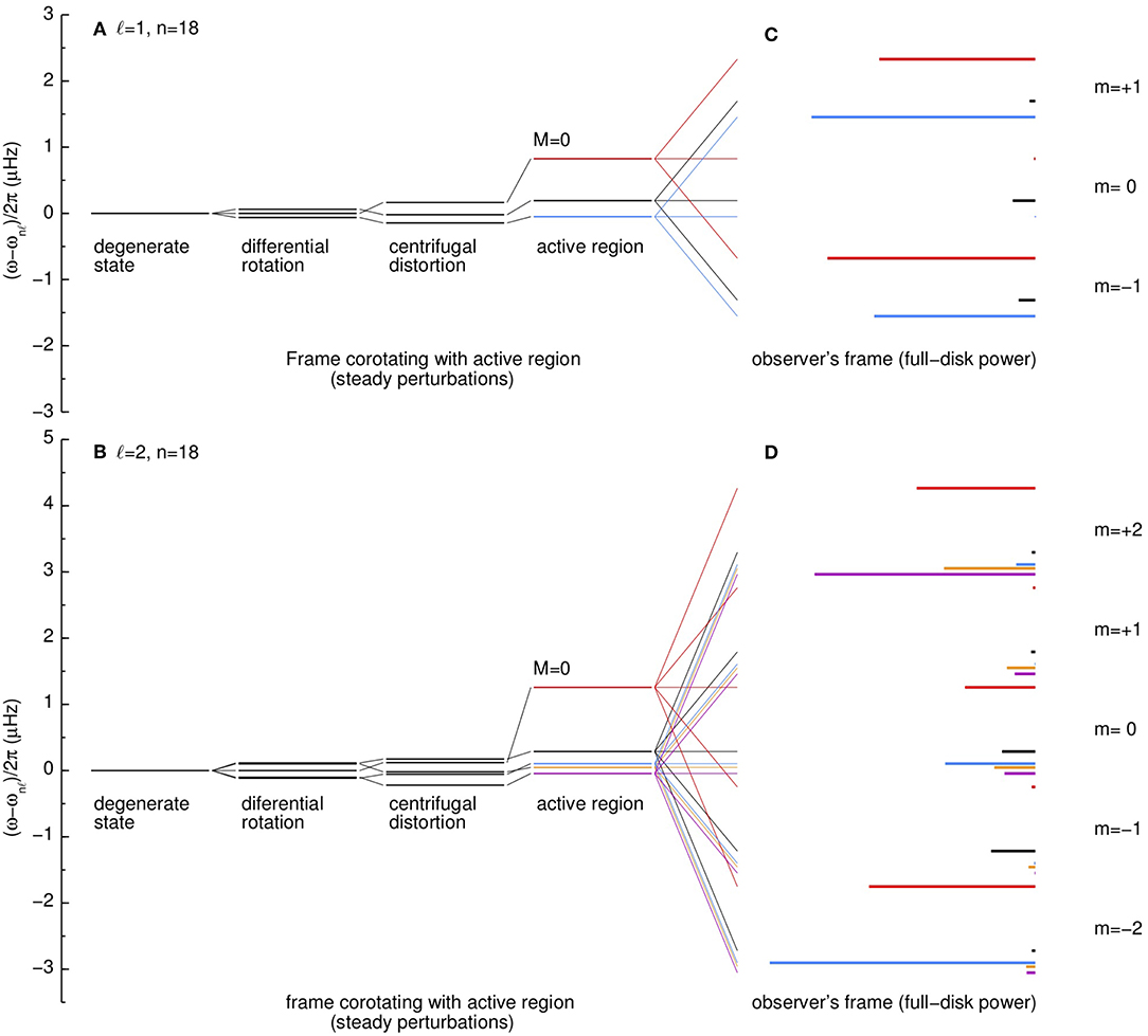
Figure 3. Perturbations to the mode eigenfrequencies in the frame that is corotating with the active region, for the multiplets with (ℓ, n) = (1, 18) (A) and with (ℓ, n) = (2, 18) (B). The star is Sun-like and rotates with a scaled solar differential rotation profile (rotation period is approximately 8 days). The active region perturbation is specified by εnℓ = 0.003, α = 23°, and β = 80°. The rotational frequency of the active region at colatitude β is Ωβ/2π is 1.504 μHz. The frequency of the mode M = 0 is the most shifted. (C,D) The (2ℓ + 1)2 peaks of the power spectrum as seen in the observer's frame, for an inclination angle i = 80°. For each m, the M-components are identified with different colors: red for M = 0, black for M = 1, blue for M = −1, orange for M = 2, and pink for M = −2. The peaks with the same colors are statistically correlated to each other (according to Equation 66).
Figure 3 also displays the different contributions to the frequency splittings due to rotation and to the active region perturbation in the corotating frame . For both multiplets, the M = 0 peaks are shifted by the largest amount, they are the most affected by the AR perturbation and in the frame (see also Papini et al., 2015). This feature, which arises from geometrical considerations only, is preserved in the spectrum as seen in the observer's frame, where the M = 0 peaks are clearly visible. With increasing AR surface coverage the frequency shifts of the M ≠ 0 modes increase and the peaks get less clustered.
3. Results
3.1. Dipole and Quadrupole Power Spectra
In this section we describe the changes imprinted by a large active region in the spectrum of two multiplets with (ℓ, n) = (1, 18) and (2, 18), for a star rotating with a period of 8 days.
Figure 4 shows the results for the quadrupole multiplet, for four combinations of the values of α and β selected in section 2.2: the observed power spectra are plotted for two angles of observation, i = 30° and 80°, and are normalized with respect to V2, i.e., with respect to the m = 0 peak of the pure rotational spectrum seen with i = 0. The corresponding theoretical Lorentzian envelope (solid line) has been calculated from Equation (36), by setting a value for the FWHM of Γ/2π = 1 μHz, typical for this multiplet in the Sun (see e.g., Chaplin et al., 2005). Due to the finite lifetime of the modes of oscillation, it is clear that is not possible to resolve all the (2ℓ + 1)2 peaks, and an observer would identify not many more than (2ℓ + 1) peaks in a multiplet. In the cases shown here, it is possible to identify from 5 to 6 peaks for i = 80°, the additional peak coming from the uppermost shifted m = 2, M = 0 peak. We note that the Lorentzian envelope displays an asymmetric profile. Because of their large shift in frequency, the M = 0 peaks blend with peaks from different m-quintuplets. This blending increases with activity level. Figure 4A shows a case for which the (M, m) = (0, 0) and (M, m) = (1, 1) peaks have close frequencies and comparable amplitudes, they contribute equally to a single peak in the power spectrum.
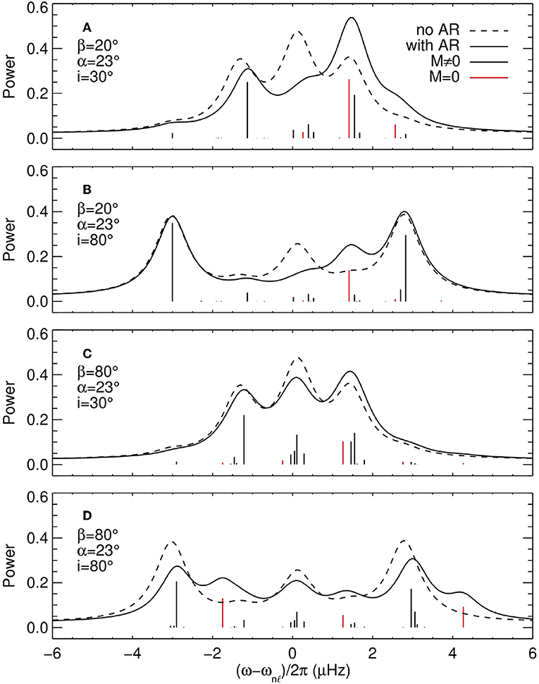
Figure 4. Oscillation power spectra for the (ℓ, n) = (2, 18) multiplet observed at two inclination angles i = 30°(A,C) and 80°(B,D), for a star with a rotation period of 8 days and for an active region with εnℓ = 0.003, β = 20°(A,B) or 80°(C,D), and for a surface coverage with α = 23°. The power spectra are normalized with respect to V2 (Equation 33). The vertical line segments show the theoretical frequencies and amplitudes for the M = ±1, ±2 modes (black) and the M = 0 mode (red). The envelopes of the power spectra (solid black curves) are obtained by summing over Lorentzians with widths of 1 μHz. The dashed black curve shows the envelope of the pure rotational power spectrum, which includes the centrifugal distortion (Equation 17).
The envelope of the power spectrum is very sensitive to the latitudinal position of the AR and to the inclination angle: in Figure 4C the power spectrum is near the standard rotationally-split spectrum, while the same configuration observed from a different inclination angle (Figure 4D) shows a more asymmetric profile with additional peaks. This is better seen in Figure 5, which shows contours of the acoustic power as a function of inclination angle, for both the ℓ = 1 and ℓ = 2 multiplets, for the same active region parameters as in Figure 4. For an active region at high latitude (middle panels of Figure 5), the central peak shows a significant shift and overlaps with the m = 1 peak. For a low-latitude active region (bottom panels) the envelope of the power spectrum displays more than 2ℓ + 1 peaks. A distinct feature is the presence of two peaks instead of one when observing an ℓ = 2 multiplet at zero inclination angle. The sensitivity of the spectrum to the colatitude of the AR, shown in Figure 6, is due in part to the variation with β of the non-diagonal elements of the rotation matrix R(ℓ).
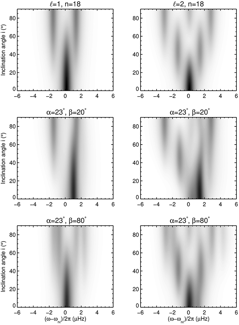
Figure 5. Expectation value of power spectra of oscillation, as functions of inclination angle i. The left panels are for the dipole multiplet ℓ = 1, n = 18, and the right panels for the quadrupole multiplet ℓ = 2, n = 18. The top panels are for the pure-rotation case, the middle panels are for an active region at colatitude β = 20°, and the bottom panels for β = 80°. The active region parameters are εnℓ = 0.003, α = 23°, and the stellar rotation period is 8 days.
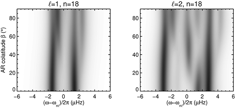
Figure 6. Expectation value of power spectra of oscillation, as functions of active-region colatitude β, at fixed inclination angle i = 80°. The other physical parameters are the same as in Figure 5.
An observed power spectrum is, of course, much more difficult to interpret than its expectation value. The power spectrum in Figure 7 includes realization noise due to the stochastic nature of stellar oscillations and to additional shot noise. At each frequency the observed power is a realization of an exponential distribution (a chi-squared with two degrees of freedom) with standard deviation and mean equal to the expectation value of the power spectrum. Realization noise considerably degrades the spectrum, however in some cases it is still possible to distinguish between the pure rotational spectrum and a spectrum with the active region.
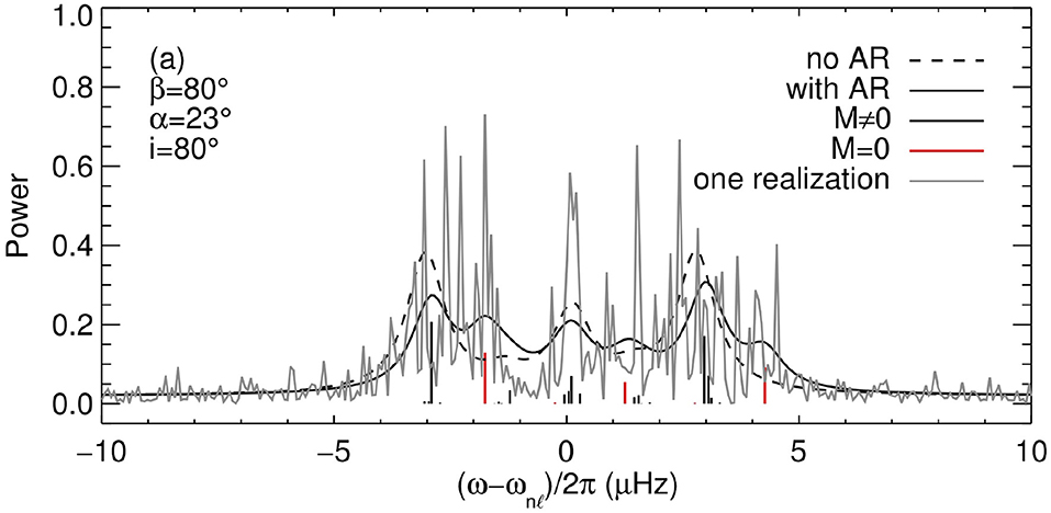
Figure 7. A realization of the power spectrum of an ℓ = 2 multiplet (gray) and its expectation value (black solid curve, also shown in Figure 4D). The observation duration is 6 months and the signal-to-noise ratio is 50. The dashed black curve shows the expectation value of the pure rotational spectrum.
3.2. Asymptotics
3.2.1. Limit of Small Latitudinal Differential Rotation
The examples shown so far suggest that the power spectrum of a multiplet may be approximated by the sum of 2(2ℓ + 1) peaks, for two reasons. First, in the corotating frame the splitting due to rotation is small compared to the shift induced by the AR perturbation (see e.g., Figure 3). Second, the AR perturbation induces a shift that is largest for the M = 0 mode. Therefore, for each m, all the M ≠ 0 peaks are clustered near the pure rotational frequencies and appear as a single peak, while the M = 0 peaks are well separated.
Here we wish to find an approximation for the power spectrum of a multiplet in terms of 2(2ℓ + 1) Lorentzians only. In the following we assume the rotation perturbation to be small compared to the active region perturbation, and seek an approximate solution to the eigenvalue problem (14).
It is convenient to solve the eigenvalue problem in the frame where the dominant perturbation is diagonal, i.e., the frame of the active region. The following results are similar to section 19.5 of Unno et al. (1989). We rewrite the elements of the full matrix in as
where the term with the sum in the right hand side correspond to . We look for solutions of the form
and
where are the perturbations to the (partially degenerate) eigenvalues and eigenvectors of , with . The eigenvector perturbation is orthogonal to the reference eigenspace (see e.g., Messiah, 1960, p. 687),
which gives The eigenvectors AM in the frame are given by
via the rotation matrix R(ℓ) (see Equation 16).
To first order, the eigenvalue problem (Equation 14) becomes
where I is the identity matrix. To calculate and we multiply the above equation on the left by the transpose of to obtain:
We find the perturbed eigenvalues by setting m′ = M in the above equation
The non-zero elements of AM, (1) are obtained from the m′ ≠ ±M components of Equation (45):
The explicit expressions for the eigenvalues and eigenvectors of the combined perturbations are
and
The explicit expression for the amplitudes in the frame is then.
3.2.2. Neglecting Latitudinal Differential Rotation
If we neglect differential rotation then Equation (18) reduces to
Then, by using the identities (Unno et al., 1989; Gough and Thompson, 1990)
and
the frequency shifts (Equation 48) simplify to
Note that for moderately fast rotating stars the Coriolis term in the above equation is much smaller than the centrifugal distortion term (e.g., Gizon and Solanki, 2004).
Due to the clustering of the M ≠ 0 peaks, the power spectrum in the observer's frame can be approximately modeled by 2(2ℓ + 1) Lorentzians, some of which may overlap. Half of these correspond to the peaks with M = 0. The remaining 2ℓ + 1 (approximate) Lorentzians are obtained by summing over the M ≠ 0 peaks; their mean frequency shifts are given by a power weighted average of the M ≠ 0 frequency shifts . We denote by 〈δω〉m this average:
with
The corresponding averaged power amplitudes 〈P〉m are (see Equation 38)
Figure 8 shows how good is the 2(2ℓ + 1)-Lorentzian model in reproducing the expected power spectrum for the case of Figure 7. The vertical red lines are for the (2ℓ + 1) peaks with M = 0, while the vertical black lines refer to the (2ℓ + 1) peaks with power 〈P〉m and frequency shifts 〈δω〉m. The envelope of power of the 2(2ℓ + 1)-model compares well with the envelope obtained by summing over all the (2ℓ + 1)2 peaks.
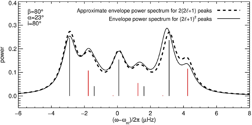
Figure 8. Acoustic power spectrum for the same case as in Figure 4D, (black solid line) and the power spectrum resulting from neglecting differential rotation and by assuming a small rotation perturbation with respect to the AR perturbation (black dashed line), as calculated from Equations (50, 51, 54). Vertical red lines denote the M = 0 peaks, and black lines the averaged M ≠ 0 peaks from Equations (55, 57).
Figure 9 shows the frequency shifts 〈δω〉m (black lines) and the shifts of the M = 0 peaks (red lines) calculated from the solution of Equation (14) (solid lines) and from the approximate solutions (dashed lines), as a function of stellar rotation rate and for an active region with a surface coverage of 4% (α = 23°) and β = 80°. The linear approximation successfully returns the frequency shifts of the 2(2ℓ + 1) Lorentzians, even for moderately high rotation rates.
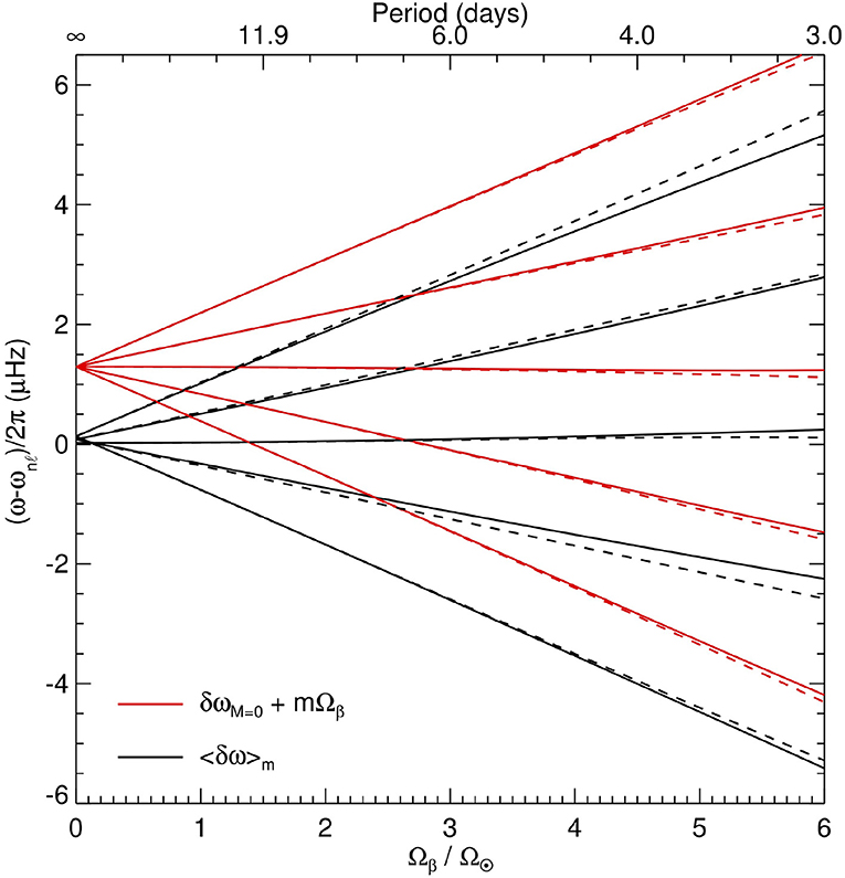
Figure 9. Black lines: Averaged frequency shifts 〈δω〉m vs. stellar rotation rate, as given by Equation (55) and calculated using Equation (14) (solid lines) and using the approximations of Equations (50, 51, 54) (dashed lines). Red lines: Approximate frequency shifts δωM = 0+mΩβ of the M = 0 peaks as given by Equation (54) (dashed lines) and first-order shifts (solid lines).
3.2.3. Limit of Small-Size Active Region (α ≲ 15°)
The above formulae for the frequency shifts simplify further when the active region has a small surface area. For small values of α, the integral in Equation (21) can be approximated,
such that becomes
As shown in Figure 2, the above approximation is very good for α ≲ 15° and ℓ ≤ 2. Up to order α2, the active region induces a shift only in the frequency of the M = 0 mode
Perturbed frequency shifts and amplitudes are obtained by following the calculation described in section 3.2.1, but taking into account the fact that the eigenfrequencies are now degenerate for M ≠ 0. The frequencies in the observer's frame can then be approximated by
where
The peak amplitudes in the power spectrum, , are given by Equation (38), where is replaced by
with
Figure 10 shows the frequency error in μHz introduced by the small-α approximation. Dark blue shades indicate the regions in parameter space (α and Ωβ) where the approximation is very good. For an active region with a surface coverage below 2%, i.e., α <15°, the frequency shift is within ~ 0.1μHz of δωM = 0, even for fast rotation rates.
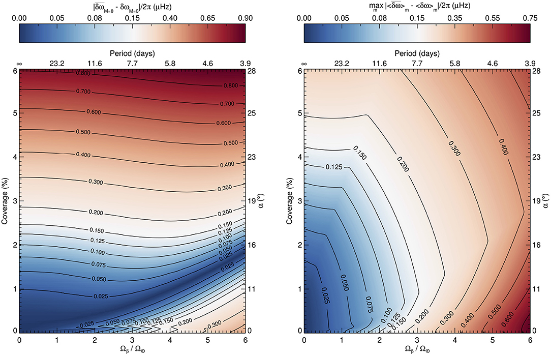
Figure 10. (Left) Contour plot of the absolute difference between the approximate shifts (see Equation 62) and the first-order shifts δωM = 0, as a function of stellar rotation rate and surface coverage of the active region. (Right) Contour plot of the maximum of the absolute difference over all values of m, as a function of stellar rotation rate and surface coverage of the active region.
3.3. Correlations in Frequency Space
Due to the fact that the active region perturbation is unsteady in the observer's frame, the intensity fluctuations (Equation 32) are not statistically independent in frequency space. Given two frequencies ω and ω′, the intensity covariance is
To simplify the analysis we assumed that is an integer (this is not a weakness of the theory though). The above expression vanishes unless |k| ≤ 2ℓ. The quantities Iobs(ω) and are correlated for frequency separations .
The power spectrum is also correlated for . Using the formulae given in appendix C of Fournier et al. (2014), we find
where the intensity covariance is given above. We note that the values of the intensity and power spectrum covariances (Equations 65 and 66) depend on the parameters of the model. However the existence of a correlation is a general feature, which arises from the fact that the active region rotates with the star. Remarkably, the expectation value of the power spectrum (ω) (see Equation 36) is as if all the terms in Equation (32) were statistically independent.
4. Discussion
4.1. Non-linear Frequency Shifts and Amplitudes From Numerical Simulations
In order to compare with the perturbation theory, we study the non-linear regime by means of numerical simulations. We use the GLASS wave propagation code, with the same numerical setup employed by Papini et al. (2015).
4.1.1. Rotation in Post-processing
Running different numerical simulations for different values of β and different perturbation amplitudes is computationally expensive. Instead we performed simulations for a 3D polar perturbation to the sound speed and for a star with no rotation, that is equivalent to solve the numerical problem in the reference frame . We introduced the effect of rotation later in processing the output. This approach has the advantage that, for a given amplitude of the AR perturbation, we only need to run one simulation in order to calculate the power spectrum for any given value of β and rotation period. However we can only reproduce solid body rotation, and it is not possible to include the effects of the centrifugal distortion and of the Coriolis force, therefore in each nℓ-multiplet we expect to find only (2ℓ + 1)(ℓ + 1) peaks. Nonetheless the results are useful for exploring the non-linear regime. We note that, as a consequence of neglecting these rotational effects, M can be identified with the azimuthal degree of the spherical harmonics in the frame (see section 2.1.1).
4.1.2. Sound-Speed Perturbation
As was done earlier, we approximate the perturbation introduced by the starspot by a local increase in sound speed. We consider separable perturbations in the square sound speed of the form
where ϵ > 0 is a positive amplitude, f is a radial profile, and g a latitudinal profile. Explicitly, g = 1/2 + cos(κθ)/2 is a raised cosine for 0 ≤ κθ < π and is zero otherwise, where π/(2κ) = 0.65 rad = 37.5°. The function is a Gaussian function centered at radius rc = 0.9985 R⊙ with dispersion σ = 0.004 R⊙, multiplied by a raised cosine. This functional form is the same as the one described by Papini et al. (2015). The perturbation is thus placed along the polar axis at a depth of 4 Mm, with a surface coverage of 12%.
4.2. Synthetic Power Spectrum
As in section 2.3, we assume that the intensity fluctuations are proportional to the Eulerian pressure perturbation measured at r0 = R + 200 km above the surface (see Papini et al., 2015). To calculate the expectation value of the observed power spectrum, we performed a first set of simulations for which all the modes were excited with the same phase at the initial time.
The approximation that the changes in the eigenfunction of a mode M are limited to the same angular degree ℓ (Equation 3) does not hold in the non-linear case: the horizontal shape of an eigenfunction is a combination of spherical harmonics of different ℓ values. However, since the perturbation is axisymmetric (see Equation 67), the eigenfunction for a mode M is a combination of spherical harmonics of different angular degree ℓ and same M. Therefore the intensity fluctuations due to all the modes with the same M take the form
where pℓM(r0, t) are the coefficients of the spherical harmonic decomposition of the pressure wavefield returned by the GLASS code in the frame . The index ℓmax is set by the spectral resolution of the spherical harmonic transform.
To obtain the full-disk integrated intensity in the observer's frame we express each in terms of the spherical harmonics in the frame
by means of two consecutive rotations of the Euler angles (0, −i, Ωβt) and (0, β, 0). Combining this equation with Equation (68) and integrating over the visible disk, we obtain the full-disk integrated intensity of each mM-component:
We then perform a Fourier transform to calculate the intensity ImM(ω) in the frequency domain. Finally, we derive the expression for the expectation value of the power spectrum
that is analogous to Equation (36), but for the entire wavefield.
For the non-linear study we chose three perturbation amplitudes ϵ = 0.1, 0.2, and 0.3 which, for the multiplet (ℓ, n) = (2, 18), correspond to ϵnℓ ≃ 0.005, 0.010, and 0.015, i.e., roughly twice to six times the value used in the linear analysis. The simulations run for 80 days (stellar time), in order to reach an accuracy of ~ 0.14 μHz in the frequency domain. The wavefield computed by GLASS includes some numerical damping that increases with frequency with an exponential dependence. We took advantage of this damping and selected two ℓ = 2 multiplets: one with n = 18 and a FWHM comparable to the solar value, the other with n = 12 and a FWHM small enough to resolve all the mM peaks in the multiplet. Model S is convectively stabilized (Papini et al., 2014), which implies that the unperturbed frequencies of the quadrupole modes are 1970.50 μHz for n = 12 and 2783.62 μHz for n = 18. Figure 11 shows the observed power spectra of the two selected multiplets in the case β = 80° and i = 80°, normalized with respect to the highest M ≠ 0 peak. In the case ϵ = 0.1, the simulated power spectrum (black curve) of the (ℓ, n) = (2, 12) multiplet (top left panel) is well reproduced by the power spectrum computed with linear theory (red dot-dashed curves), except for the peaks corresponding to M = 0 (vertical red curves show the M = 0 peaks from linear theory), which are less shifted in frequency and have smaller amplitudes than predicted. For the (ℓ, n) = (2, 18) multiplet (top right panel) the non-linear effects are less visible, due to the overlapping Lorentzian profiles. A blue curve, displaying the contribution to the power spectrum of the M = 0 peaks, shows that also for this multiplet the M = 0 component of the power spectrum deviates from the linear behavior, both in frequency and amplitude. This plot also shows an example of the combined action of mode mixing and mode visibility, which almost suppresses the m = 0, M = 0 peak located at a frequency shift of ~ 3.1 μHz.
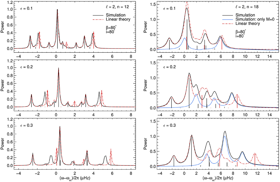
Figure 11. Numerical simulations of oscillation power spectra for two quadrupole multiplets with n = 12 (left panels) and n = 18 (right panels), for an inclination angle i = 80° and a stellar rotation period of 8 days (solid body rotation). The active region has a colatitude β = 80° and different perturbation amplitudes of ϵ = 0.1 (top), 0.2 (middle), and 0.3 (bottom), with rc = 0.9985R⊙, σ = 0.004R⊙, and κ = 2.4 (see Equation 67). The black curves show the power spectra computed with the GLASS code, the red dot-dashed curves indicate the power spectra computed using linear perturbation theory. Vertical lines show the peaks from linear theory, in red for M = 0 and in black M ≠ 0. The blue curves in the right panels display the contribution of the M = 0 peaks to the simulated power spectrum. The n = 12 peaks have a FWHM of Γ/2π ≃ 0.2 μHz, while for n = 18 the peaks have Γ/2π ≃ 1 μHz.
With increasing ϵ (middle and bottom panels) the interaction of the wavefield with the active region becomes strongly non-linear, and for a perturbation with ϵ = 0.3 results in a massive distortion of the power spectrum with respect to that one predicted by linear theory. Here two different behaviors are evident: in the (ℓ, n) = (2, 12) multiplet the m = 0, M = 0 peaks are almost suppressed, while the peak with m = 0, M = 0 in the (ℓ, n) = (2, 18) multiplet, that was suppressed in the case ϵ = 0.1, increases in amplitude as ϵ increases (middle and bottom right panels). Moreover the peaks with M = 1 start to deviate from the linear prediction. This is in agreement with what found in the non-rotating case by Papini et al. (2015), who also showed that second-order perturbations would correct most of the differences.
4.3. Correlations in Synthetic Power Spectra
In section 3.3 we showed that in presence of an active region rotating with the star, the power spectrum of a multiplet is correlated at frequency separations that are multiple of the rotational frequency of the active region. However, for small perturbations this correlation is too weak to be observed. Here we ask whether such a correlation can be measured in presence of a perturbation of moderate amplitude. For that purpose, we ran a second set of simulations, in which the acoustic waves were excited by applying a random forcing function at 150 km below the surface at each time step, as described by Hanasoge and Duvall (2007). The duration of the simulation is 80 days (stellar time). In the frequency domain, the observed intensity is
where ImM(ω) is obtained by Fourier transformation of Equation (70) using the numerical realizations of pℓM(r0, t).
The autocorrelation of the intensity spectrum is
where [ωnℓ] denotes an appropriate frequency interval of size ~ 20 μHz containing the multiplet nℓ but excluding the nearby l = 0 mode. The average is performed over all ℓ = 2 multiplets with n ranging from 15 to 25.
Figure 12 shows the real part of CI for the special case of an inclination angle i = 80° and a starspot at colatitude β = 80° with ϵ = 0.1. A correlation is clearly visible at frequency separations Δω = 2Ωβ and 4Ωβ. This suggests that the frequency-domain autocorrelation function could be used as a diagnostic tool to identify unsteady perturbations in the time series of stellar oscillation. We note that the imaginary part of CI contains no visible signal above the noise level.
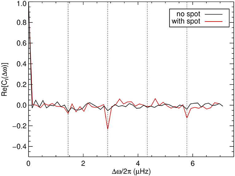
Figure 12. Autocorrelation of the intensity power spectrum as defined by Equation (73) for a starspot with ϵ = 0.1 (red curve). A stellar rotation period 2π/Ωβ = 8 days, an inclination angle i = 80°, and a starspot colatitude β = 80° were chosen for the post processing. Vertical dotted lines denote frequency separations Δω = jΩβ where j = 1, 2, 3, 4. For comparison, the black curve is the case with no starspot.
4.4. Toward a Physical Model for Mode Interaction With an Active Region
In this paper we replaced the active region by a localized increase in sound-speed near the stellar surface. We focused on the geometrical aspects of the problem rather than on the physics. One may ask, however, what would be the difference in the obtained results if we had instead considered a realistic model for the magnetic active region. Although we will not answer this question here, it is worth listing some of the steps involved.
A typical solar active region consists of a pair of sunspots surrounded by plage with strong vertical field. Local helioseismology of the visible disk and the far side indicates that p modes are strongly scattered by both sunspots and extended plage (see e.g., Gizon et al., 2009, and references therein). Some studies of the interaction of high-degree p modes with magnetostatic sunspots (e.g., Moradi et al., 2010; Cameron et al., 2011) have been carried out using MHD wave propagation codes (Cameron et al., 2008; Felipe et al., 2016). Other studies are based on numerical magneto-convective simulations (e.g., Rempel et al., 2009; DeGrave et al., 2014). The main conclusion of these simulations is that the interaction takes place in the top few hundred kilometers below the surface, where the direct effects of the magnetic field and the indirect effects due to changes in thermodynamic structure with respect to the reference atmosphere (e.g., the Wilson depression) are large. Wave simulations indicate that the outgoing p modes are phase shifted with respect to the incoming p modes in such a way that the effective wave speed is increased, as observed. The physical interaction involves the conversion of p modes into fast and slow magnetoacoustic modes in the sunspot (e.g., Khomenko and Collados, 2006; Cameron et al., 2008). A fraction of the incoming p-mode energy is tunneled downward in the form of slow MHD waves, leading to absorption (Braun, 1995; Zhao and Chou, 2016). See also, e.g., Saio and Gautschy (2004) and Cunha (2006) for mode conversion calculations in roAp stars.
Using 2D ray tracing, Liang et al. (2013) showed that high-degree helioseismic waveforms can be reproduced by increasing the effective wave speed by 10% in the sunspot. This provides some justification for the values that we have used in the present paper, although the extension to low-degree p modes has not been studied. Clearly, much additional work will be needed to determine the correct active-region perturbation amplitude from first principles. Until then, a simple calibration can be obtained from the observational study by Santos et al. (2016) who estimated empirically the contribution of sunspots to the low-degree p-mode frequency shifts associated with the solar cycle. By combining our Equation (20) with Equation (3) from Santos et al. (2016), we find εnℓ = −Δδch/Iℓ, where Δδch is the integral phase difference introduced in the mode eigenfunction by a sunspot and Iℓ is related to mode inertia. Using the value Δδch = −0.44 estimated by Santos et al. (2016), we have εnℓ ~ 0.05 for a quadrupole mode, i.e., a larger value than proposed by Liang et al. (2013) and used in the present paper. This may suggest that for large active regions the spectra calculations may have to be carried out in the non-linear regime. However, only realistic numerical modeling would help settle this question. The full problem would also have to include multiple scattering by collections of flux tubes in plage (see e.g., Hanson and Cally, 2015).
5. Conclusions
In this paper we investigated the changes in global acoustic oscillations caused by a localized sound-speed perturbation on a rotating star mimicking a large active region, using both linear perturbation theory and 3D numerical simulations. In an inertial frame, the active region perturbation is unsteady.
We find that the power spectra of low-degree modes have a complex structure. The combined effects of the active region and differential rotation cause each nℓ-multiplet to appear as (2ℓ + 1)2 peaks, each with a different amplitude. Most of the peaks are clustered near the classical rotationally-split frequencies, and only 2ℓ + 1 peaks (the M = 0 peaks, which correspond to the axisymmetric mode in the reference frame of the AR) are shifted to higher frequencies. This leads to an apparent asymmetry in the line profiles. However, due to the finite lifetime of acoustic oscillations, most of the peaks cannot be resolved. For solar-type stars, the results are not very sensitive to the choice of latitudinal differential rotation profile.
The structure of the power spectra is sensitive to the latitudinal position of the active region and to the inclination angle i of the stellar rotation axis. The latter plays a major role in determining the relative visibility of the individual peaks. We find that the envelope of the power spectrum becomes more complex as the latitude of the active region decreases. In practice, it would be very difficult to perform a fit of the (2ℓ + 1)2 peaks in a multiplet, due to peak blending and noise. However, by neglecting differential rotation it is possible to derive a simplified formula that approximates the power spectrum of a multiplet to a sum of only 2(2ℓ + 1) Lorentzian profiles. For small-area active regions, the formula further simplifies and directly links the frequencies of the peaks in the power spectrum to the active region parameters. Such formula may find applications in the analysis of real asteroseismic observations.
Numerical simulations were performed to explore the non-linear regime of the perturbation. We find that the M = 0 peaks deviate from the linear behavior for active-region perturbation amplitudes εnℓ ≳ 0.005. Depending on each particular case, the amplitude of these peaks is either reduced or enhanced compared to first-order linear theory, due to mixing with modes with other values of ℓ and m (Papini et al., 2015).
We found that there are correlations in the power spectrum at frequency separations that are multiples of the active-region rotation rate. In the linear regime the correlation signal is too weak to be observed. However the numerical simulations show that for active-region perturbations of moderate amplitude, such a correlation might be detectable, provided that the frequency intervals are carefully selected to increase the signal to noise ratio.
We note that perturbation theory can easily be extended to compute the effect of multiple active regions provided that latitudinal differential rotation is small. The treatment of several active regions rotating at different rotation rates would require a different setup, since there is no frame in which these perturbations are steady. A numerical approach would be preferable in such a case.
The work presented in this paper uses simplified physics, but it should provide useful guidance to identify the seismic signature of a large active region in the power spectrum of stellar oscillations. Given that the values of ϵnℓ are uncertain, we believe that it is worth searching for low-degree multiplets consisting of 2(2ℓ + 1) components in available asteroseismic observations. Ideal targets are stars that are known to have high-quality oscillation power spectra (high SNR, narrow lineprofiles, clear rotational splitting, see e.g., Nielsen et al., 2014) and show evidence for long-lived starspots (e.g., Nielsen et al., 2013, 2019). The catalog of potential targets, currently limited to CoRoT and Kepler, will increase fast with TESS (Ricker et al., 2015) and PLATO (Rauer et al., 2014).
Author Contributions
LG provided the basic theory. EP provided the numerical applications. Both authors contributed to the analysis of the results and to the writing of the article.
Conflict of Interest
The authors declare that the research was conducted in the absence of any commercial or financial relationships that could be construed as a potential conflict of interest.
Acknowledgments
This paper is a contribution to PLATO PSM activity Seismic diagnostics of stellar activity. We acknowledge financial support from the German Aerospace Center DLR and from the Max Planck Society. We thank Shravan Hanasoge for making the GLASS code available. Computational resources were provided by the German Data Center for SDO. This work appeared in part in the Ph.D. thesis of Papini (2016).
References
Aerts, C., Christensen-Dalsgaard, J., and Kurtz, D. W. (2010). Asteroseismology. Dordrecht: Springer.
Anderson, E. R., Duvall, T. L. Jr., and Jefferies, S. M. (1990). Modeling of solar oscillation power spectra. Astrophys. J. 364, 699–705. doi: 10.1086/169452
Bigot, L., and Dziembowski, W. A. (2002). The oblique pulsator model revisited. Astron. Astrophys. 391, 235–245. doi: 10.1051/0004-6361:20020824
Braun, D. C. (1995). Scattering of p-Modes by sunspots. I. Observations. Astrophys. J. 451:859. doi: 10.1086/176272
Cameron, R., Gizon, L., and Duvall, T. L. J. (2008). Helioseismology of sunspots: confronting observations with three-dimensional MHD simulations of wave propagation. Solar Phys. 251, 291–308. doi: 10.1007/s11207-008-9148-1
Cameron, R. H., Gizon, L., Schunker, H., and Pietarila, A. (2011). Constructing semi-empirical sunspot models for helioseismology. Solar Phys. 268, 293–308. doi: 10.1007/s11207-010-9631-3
Chaplin, W. J., Elsworth, Y., Houdek, G., and New, R. (2007). On prospects for sounding activity cycles of Sun-like stars with acoustic modes. Mon. Not. Roy. Astron. Soc. 377, 17–29. doi: 10.1111/j.1365-2966.2007.11581.x
Chaplin, W. J., Houdek, G., Elsworth, Y., Gough, D. O., Isaak, G. R., and New, R. (2005). On model predictions of the power spectral density of radial solar p modes. Mon. Not. Roy. Astron. Soc. 360, 859–868. doi: 10.1111/j.1365-2966.2005.09041.x
Christensen-Dalsgaard, J. (2008). ADIPLS – the Aarhus adiabatic oscillation package. Astrophys. Space Sci. 316, 113–120. doi: 10.1007/s10509-007-9689-z
Christensen-Dalsgaard, J., Däppen, W., Ajukov, S. V., Anderson, E. R., Antia, H. M., Basu, S., et al. (1996). The current state of solar modeling. Science 272, 1286–1292. doi: 10.1126/science.272.5266.1286
Cunha, M. S. (2006). Improved pulsating models of magnetic Ap stars - I. Exploring different magnetic field configurations. Mon. Not. Roy. Astron. Soc. 365, 153–164. doi: 10.1111/j.1365-2966.2005.09674.x
Cunha, M. S., and Gough, D. (2000). Magnetic perturbations to the acoustic modes of roAp stars. Mon. Not. Roy. Astron. Soc. 319, 1020–1038. doi: 10.1046/j.1365-8711.2000.03896.x
DeGrave, K., Jackiewicz, J., and Rempel, M. (2014). Time-distance helioseismology of two realistic sunspot simulations. Astrophys. J. 794:18. doi: 10.1088/0004-637X/794/1/18
Dicke, R. H. (1982). The 5-min oscillations of the sun are incompatible with a rapidly-rotating core. Nature 300, 693–697. doi: 10.1038/300693a0
Dziembowski, W., and Goode, P. R. (1984). Simple asymptotic estimates of the fine structure in the spectrum of solar oscillations due to rotation and magnetism. Mem. Soc. Astron. Ital. 55, 185–213.
Dziembowski, W., and Goode, P. R. (1985). Frequency splitting in AP stars. Astrophys. J. 296, L27–L30. doi: 10.1086/184542
Dziembowski, W. A., and Goode, P. R. (1992). Effects of differential rotation on stellar oscillations - A second-order theory. Astrophys. J. 394, 670–687. doi: 10.1086/171621
Felipe, T., Braun, D. C., Crouch, A. D., and Birch, A. C. (2016). Helioseismic holography of simulated sunspots: magnetic and thermal contributions to travel times. Astrophys. J. 829:67. doi: 10.3847/0004-637X/829/2/67
Fournier, D., Gizon, L., Hohage, T., and Birch, A. C. (2014). Generalization of the noise model for time-distance helioseismology. Astron. Astrophys. 567:A137. doi: 10.1051/0004-6361/201423580
García, R. A., Mathur, S., Salabert, D., Ballot, J., Régulo, C., Metcalfe, T. S., et al. (2010). CoRoT reveals a magnetic activity cycle in a sun-like star. Science 329:1032. doi: 10.1126/science.1191064
Gizon, L. (1995). “Can we see the back of the sun?,” in Proceedings of the Solar and Terrestrial Energy Program (STEP) 1995 Conference, eds R. A. Vincent and I. M. Reid (Adelaide, SA: University of Adelaide) 173–176.
Gizon, L. (1998). “Comments on the influence of solar activity on p-mode oscillation spectra,” in New Eyes to See Inside the Sun and Stars, volume 185 of IAU Symposium, eds F.-L. Deubner, J. Christensen-Dalsgaard, and D. Kurtz (Dordrecht: Kluwer), 173.
Gizon, L. (2002). Prospects for detecting stellar activity through asteroseismology. Astron. Nachrichten 323, 251–253. doi: 10.1002/1521-3994(200208)323:3/4<251::AID-ASNA251>3.0.CO;2-9
Gizon, L., Birch, A. C., and Spruit, H. C. (2010). Local helioseismology: three-dimensional imaging of the solar interior. Ann. Rev. Astron. Astrophys. 48, 289–338. doi: 10.1146/annurev-astro-082708-101722
Gizon, L., Schunker, H., Baldner, C. S., Basu, S., Birch, A. C., Bogart, R. S., et al. (2009). Helioseismology of sunspots: a case study of NOAA region 9787. Space Sci. Rev. 144, 249–273. doi: 10.1007/s11214-008-9466-5
Gizon, L., Sekii, T., Takata, M., Kurtz, D. W., Shibahashi, H., Bazot, M., et al. (2016). Shape of a slowly rotating star measured by asteroseismology. Sci. Adv. 2:e1601777. doi: 10.1126/sciadv.1601777
Gizon, L., and Solanki, S. K. (2004). Measuring stellar differential rotation with asteroseismology. Solar Phys. 220, 169–184. doi: 10.1023/B:SOLA.0000031378.29215.0c
Goode, P. R., and Thompson, M. J. (1992). The effect of an inclined magnetic field on solar oscillation frequencies. Astrophys. J. 395, 307–315. doi: 10.1086/171653
Gough, D. O., and Taylor, P. P. (1984). Influence of rotation and magnetic fields on stellar oscillation eigenfrequencies. Mem. Soc. Astron. Ital. 55, 215–226.
Gough, D. O., and Thompson, M. J. (1990). The effect of rotation and a buried magnetic field on stellar oscillations. Mon. Not. Roy. Astron. Soc. 242, 25–55. doi: 10.1093/mnras/242.1.25
Hanasoge, S. M., and Duvall, T. L Jr.. (2007). The solar acoustic simulator: applications and results. Astronom. Nach. 328, 319–322. doi: 10.1002/asna.200610737
Hansen, C. J., Cox, J. P., and van Horn, H. M. (1977). The effects of differential rotation on the splitting of nonradial modes of stellar oscillation. Astrophys. J. 217, 151–159. doi: 10.1086/155564
Hanson, C. S., and Cally, P. S. (2015). Multiple scattering of seismic waves from ensembles of upwardly lossy thin flux tubes. Solar Phys. 290, 1889–1896. doi: 10.1007/s11207-015-0732-x
Khomenko, E., and Collados, M. (2006). Numerical modeling of magnetohydrodynamic wave propagation and refraction in sunspots. Astrophys. J. 653, 739–755. doi: 10.1086/507760
Kiefer, R., Schad, A., Davies, G., and Roth, M. (2017). Stellar magnetic activity and variability of oscillation parameters: an investigation of 24 solar-like stars observed by Kepler. Astron. Astrophys. 598:A77. doi: 10.1051/0004-6361/201628469
Kurtz, D. W. (1982). Rapidly oscillating AP stars. Mon. Not. Roy. Astron. Soc. 200, 807–859. doi: 10.1093/mnras/200.3.807
Kurtz, D. W. (2008). The solar-stellar connection: magneto-acoustic pulsations in 1.5 M⊙ – 2 M⊙ peculiar A stars. Solar Phys. 251, 21–30. doi: 10.1007/s11207-008-9139-2
Kurtz, D. W., and Shibahashi, H. (1986). An analysis of the ℓ = 1 dipole oscillation in HR 3831 (HD 83368). Mon. Not. Roy. Astron. Soc. 223, 557–579. doi: 10.1093/mnras/223.3.557
Ledoux, P. (1951). The nonradial oscillations of gaseous stars and the problem of beta canis majoris. Astrophys. J. 114:373. doi: 10.1086/145477
Liang, Z. C., Gizon, L., Schunker, H., and Philippe, T. (2013). Helioseismology of sunspots: defocusing, folding, and healing of wavefronts. Astron. Astrophys. 558:A129. doi: 10.1051/0004-6361/201321483
Libbrecht, K. G., and Woodard, M. F. (1990). Solar-cycle effects on solar oscillation frequencies. Nature 345, 779–782. doi: 10.1038/345779a0
Moradi, H., Baldner, C., Birch, A. C., Braun, D. C., Cameron, R. H., Duvall, T. L., et al. (2010). Modeling the subsurface structure of sunspots. Solar Phys. 267, 1–62. doi: 10.1007/s11207-010-9630-4
Mosser, B., Baudin, F., Lanza, A. F., Hulot, J. C., Catala, C., Baglin, A., et al. (2009). Short-lived spots in solar-like stars as observed by CoRoT. Astron. Astrophys. 506, 245–254. doi: 10.1051/0004-6361/200911942
Nielsen, M. B., Gizon, L., Cameron, R. H., and Miesch, M. (2019). Starspot rotation rates versus activity cycle phase: butterfly diagrams of Kepler stars are unlike that of the Sun. Astron. Astrophys. 622:A85. doi: 10.1051/0004-6361/201834373
Nielsen, M. B., Gizon, L., Schunker, H., and Karoff, C. (2013). Rotation periods of 12 000 main-sequence Kepler stars: dependence on stellar spectral type and comparison with vsini observations. Astron. Astrophys. 557:L10. doi: 10.1051/0004-6361/201321912
Nielsen, M. B., Gizon, L., Schunker, H., and Schou, J. (2014). Rotational splitting as a function of mode frequency for six Sun-like stars. Astron. Astrophys. 568:L12. doi: 10.1051/0004-6361/201424525
Pallé, P. L., Régulo, C., and Roca Cortés, T. (1989). Solar cycle induced variations of the low L solar acoustic spectrum. Astron. Astrophys. 224, 253–258.
Papini, E. (2016). Simulating the signature of starspots in stellar oscillations. (Ph.D. thesis). Georg-August-Universität Göttingen, Göttingen, Germany.
Papini, E., Birch, A. C., Gizon, L., and Hanasoge, S. M. (2015). Simulating acoustic waves in spotted stars. Astron. Astrophys. 577:A145. doi: 10.1051/0004-6361/201525842
Papini, E., Gizon, L., and Birch, A. C. (2014). Propagating linear waves in convectively unstable stellar models: a perturbative approach. Solar Phys. 289, 1919–1929. doi: 10.1007/s11207-013-0457-7
Press, W. H., Teukolsky, S. A., Vetterling, W. T., and Flannery, B. P. (1992). Numerical Recipes in FORTRAN. The Art of Scientific Computing, 2nd Edn. New York, NY: Cambridge University Press.
Rauer, H., Catala, C., Aerts, C., Appourchaux, T., Benz, W., Brandeker, A., et al. (2014). The PLATO 2.0 mission. Exp. Astron. 38, 249–330. doi: 10.1007/s10686-014-9383-4
Rempel, M., Schüssler, M., and Knölker, M. (2009). Radiative magnetohydrodynamic simulation of sunspot structure. Astrophys. J. 691, 640–649. doi: 10.1088/0004-637X/691/1/640
Ricker, G. R., Winn, J. N., Vanderspek, R., Latham, D. W., Bakos, G. Á., Bean, J. L., et al. (2015). Transiting exoplanet survey satellite (TESS). J. Astron. Telesc. Instrum. Syst. 1:014003.
Saio, H. (1981). Rotational and tidal perturbations of nonradial oscillations in a polytropic star. Astrophys. J. 244, 299–315. doi: 10.1086/158708
Saio, H., and Gautschy, A. (2004). Axisymmetric p-mode pulsations of stars with dipole magnetic fields. Mon. Not. Roy. Astron. Soc. 350, 485–505. doi: 10.1111/j.1365-2966.2004.07659.x
Santos, A. R. G., Cunha, M. S., Avelino, P. P., Chaplin, W. J., and Campante, T. L. (2016). On the contribution of sunspots to the observed frequency shifts of solar acoustic modes. Mon. Not. Roy. Astron. Soc. 461, 224–229. doi: 10.1093/mnras/stw1348
Schunker, H., Gizon, L., Cameron, R. H., and Birch, A. C. (2013). Helioseismology of sunspots: how sensitive are travel times to the Wilson depression and to the subsurface magnetic field? Astron. Astrophys. 558:A130. doi: 10.1051/0004-6361/201321485
Shibahashi, H., and Takata, M. (1993). Theory for the distorted dipole modes of the rapidly oscillating AP stars: a refinement of the oblique pulsator model. Pub. Astron. Soc. Japan 45, 617–641.
Strassmeier, K. G. (2009). Starspots. Astron. Astrophys. Rev. 17, 251–308. doi: 10.1007/s00159-009-0020-6
Toutain, T., and Gouttebroze, P. (1993). Visibility of solar p-modes. Astron. Astrophys. 268, 309–318.
Unno, W., Osaki, Y., Ando, H., Saio, H., and Shibahashi, H. (1989). Nonradial Oscillations of Stars. Tokyo: University of Tokyo Press.
Keywords: asteroseismology, stars: oscillations, stars: activity, stars: rotation, starspots
Citation: Papini E and Gizon L (2019) Asteroseismic Signature of a Large Active Region. Front. Astron. Space Sci. 6:72. doi: 10.3389/fspas.2019.00072
Received: 21 December 2018; Accepted: 04 November 2019;
Published: 06 December 2019.
Edited by:
Markus Roth, Albert Ludwigs Universität Freiburg, GermanyReviewed by:
Maria Pia Di Mauro, Istituto Nazionale di Astrofisica (INAF), ItalyAbhishek Kumar Srivastava, Indian Institute of Technology (BHU), India
Copyright © 2019 Papini and Gizon. This is an open-access article distributed under the terms of the Creative Commons Attribution License (CC BY). The use, distribution or reproduction in other forums is permitted, provided the original author(s) and the copyright owner(s) are credited and that the original publication in this journal is cited, in accordance with accepted academic practice. No use, distribution or reproduction is permitted which does not comply with these terms.
*Correspondence: Laurent Gizon, gizon@mps.mpg.de