Spatial structure of in situ reflectance in coastal and inland waters: implications for satellite validation

1 Introduction

Satellite observations of aquatic reflectance are used to derive water quality parameters such as photosynthetic pigment concentration, light availability, and infer the transport of suspended solids. These are used to delineate aquatic habitats and to investigate biogeochemical processes in aquatic ecosystems. Satellite radiance recorded at the top of the atmosphere requires correction for atmospheric scattering and absorption to provide consistent observation of water colour. Accurate derivation of the water-leaving radiance is challenging as the aquatic signal component is often $<$ 10% of the top-of-atmospheric radiance budget (Wang et al., 2009). To calibrate and validate the atmospheric correction, networks of stations measuring above-water in situ remote-sensing reflectance (R_rs) have been increasingly used to complement observations in the water column which are relatively demanding on ship time and maintenance. Validation of satellite-derived reflectance accuracy is achieved by quantifying the statistical differences with coincident in situ observations, where the latter are assumed to represent truth values within specified uncertainty bounds (Loew et al., 2017).

The atmospheric correction of satellite radiometry is particularly challenging in coastal and inland waters, due to their optical complexity relative to ocean waters where optical properties are closely coupled to the phytoplankton component. Inland and coastal waters also have pronounced diversity in their particulate constituents, and therefore the shape of reflectance spectra (Spyrakos et al., 2018; Lehmann et al., 2023). A wide turbidity range, particularly at rivers and in relatively shallow areas with soft substrate, can cause near-infrared (NIR) reflectance to depart significantly from zero, making the atmospheric correction harder to constrain than in the open ocean (Siegel et al., 2000). Near land, the top-of atmosphere radiance is further perturbed by light reflected from neighbouring land pixels and scattered into the field of view of the sensor, also known as the adjacency effect (Otterman and Fraser, 1979; Bulgarelli et al., 2014). Additionally, near the coast, there are complex aerosol mixtures that make selection of an appropriate aerosol model very challenging (e.g., Montes et al., 2022). Current satellite radiometer systems used for inland and coastal waters include those designed for ocean colour observation with a spatial resolution up to 300 m and daily revisit time, as well as land imagers with fewer and broader spectral bands but higher spatial resolution (up to 10 m) and longer revisit times up to 5 days at the equator. There are several atmospheric correction processors developed for these systems that are undergoing validation with in situ R_rs (e.g., Barnes et al., 2019; Warren et al., 2019; Pahlevan et al., 2021). Due to dependencies between water type and satellite R_rs accuracy (Pahlevan et al., 2021), it is desirable to perform satellite validation across a range of sites representing optical variability in water and atmospheric composition.

In addition to the atmospheric correction, the differing spatial scales of satellite and in situ reflectance are sources of uncertainty within a validation analysis (Salama and Su, 2011; Lee et al., 2012; Salama et al., 2022). Historically, pixel sizes for satellite aquatic remote sensing sensors were ∼ 100–1,000 m² (Groom et al., 2019), which is far greater than the meter-scale footprint of in situ R_rs. For example, ESA Sentinel-3 OLCI (Ocean Land Color Instrument) has a pixel size 300 m. More recently, higher resolution sensors such as ESA Sentinel-2 Multi Spectral Imager (MSI), which has pixel size 10–60 m, have been used for remote sensing of coastal and inland waters (Warren et al., 2019). Mobile (typically shipborne) and fixed radiometric platforms are both used to collect in situ R_rs, and the different sampling strategies impact on how spatial discrepancy with the satellite pixel can be accounted for. Validation from fixed platforms, for example, the Aeronet-OC network (Zibordi et al., 2009; 2022), is reliant on selecting spatially homogeneous sites and applying filters for spatial homogeneity (Concha et al., 2021). Mobile radiometers deployed for along-track sampling on research vessels and ships-of-opportunity have the benefit that sub-pixel averaging can quantify sub-pixel variability in the presence of horizontal heterogeneity (Brewin et al., 2016), depending on vessel speed and instrument frequency. Deploying mobile radiometers on ships-of-opportunity is a particularly attractive solution to obtaining extensive spatial sampling of inland and coastal water bodies at a low operational cost.

In addition to repeat spatial sampling within an individual pixel, mobile radiometers are also more likely to sample data within multiple satellite pixels within a match-up time window. In principle, this capacity allows for many different match-up pairs to be identified from a single satellite scene. However, validation metrics are typically based on an assumption of statistically independent observation pairs (Loew et al., 2017). Consequently, it is desirable to test for spatial autocorrelation - the statistical dependence of in situ R_rs within neighbouring pixels - prior to performing the match-up analysis. Spatial autocorrelation (in the context of match-up analysis) has received surprisingly little attention within the ocean colour research community, in part due to the relative scarcity of R_rs transects. Research into the scale-dependence of variability and spatial autocorrelation through variography is, however, relatively common in other areas of satellite validation; for example, forest (Román et al., 2009) and glacier (Ryan et al., 2017) albedo. Variography has also successfully been applied to optical water properties in different scientific contexts; for example, spatially resolving sediment plumes (Aurin et al., 2013) and investigation of the spatial structure of planktonic marine ecosystems at the mesoscale (∼10–100 km) (Glover et al., 2018).

In this study we quantify the spatial structure of in situ R_rs from mobile radiometric deployments in coastal and inland waters (Lake Balaton, Western English Channel, Tagus Estuary) over repeat transects which range from ∼ 1 km - ∼ 35 km in length. The overall goal is to provide insight on how spatial structure of in situ R_rs impacts on satellite validation and provide recommendations on how data from mobile radiometers can best be used in the future. We do not perform an explicit match-up analysis with satellite data, but instead apply variogram analysis to in situ data selected within a time interval broadly representative of a match-up window. We partition variation of in situ R_rs into spatial and intrinsic (non-spatial) components, and provide statistics across different spectral bands and deployments. We assess the variation in in situ R_rs at a length scale representative of a medium-resolution satellite sensor such as OLCI (300 m), which enables us to assess how the mobile radiometer is able to reduce in situ R_rs variability via sub-pixel sampling. We then assess the autocorrelation length of in situ R_rs; a quantity which serves as a criterion for selecting independent pixel match-ups for validation from a single scene. This study informs the process of working towards fully automated satellite validation services, specifically highlighting the role of spatial statistics when using data from mobile autonomous radiometric systems.

2 Satellite validation of remote-sensing reflectance

To motivate the study, we first present a brief review of R_rs satellite validation practice, focusing on spatial and temporal collocation. Satellite validation is defined as the process of evaluating, by independent means, the accuracy of satellite-derived data products and quantifying their uncertainties by comparison with in situ reference data (Justice et al., 2000; Loew et al., 2017). In aquatic remote sensing in situ measurements of R_rs (defined as the ratio of water-leaving radiance to downwelling planar irradiance just above the water surface), or the related variable of normalized-water leaving radiance, provide reference data for validation of satellite products (Bailey and Werdell, 2006; Zibordi et al., 2009; Qin et al., 2017; Warren et al., 2019; Pahlevan et al., 2021). R_rs from satellite sensors is normally multi-spectral, consisting of measurements in discrete spectral bands. R_rs from in situ sensors is typically hyperspectral and convolved with the spectral response function of the satellite sensor when performing validation. For convenience, we generally do not explicitly notate the wavelength-dependence of R_rs and other radiometric quantities.

2.1 Match-up criteria and validation metrics

The ocean colour community has applied a range of criteria to match-up analysis which differ primarily in quality control thresholds and spatiotemporal collocation criteria (Bailey and Werdell, 2006; Zibordi et al., 2009; Concha et al., 2021). Prior to matching with in situ data, satellite R_rs are often locally averaged (e.g., using a moving 3 × 3 average of neighbouring pixels). This spatial window, the ‘satellite extract’, is also used to test for spatial homogeneity in R_rs via the local coefficient of variation and to filter out noisy or heterogeneous regions (Bailey and Werdell, 2006). The time window is kept sufficiently short to limit spatiotemporal discrepancies between the in situ and remote sample population, or long to produce sufficient data to allow statistical analysis. The length of the temporal window about a satellite overpass that is used to select in situ R_rs has varied from ±0.5 h (Ilori et al., 2019) (highly dynamic environments) to ±1 day or greater (Kutser, 2012; Warren et al., 2019) (inland waters). Match-up windows for coastal environments typically range from ±1 h to ±3 h (refer to Table 3 in Concha et al. (2021)). Recent IOCCG recommendations for dynamic regions are ±1 h (IOCCG, 2019). If there are repeated in situ R_rs measurements within a pixel within the match-up window, these are typically averaged before being defined as a match-up pair. In addition, a sequence of quality control filters are applied to both in situ R_rs (e.g., restrictions on viewing angles, wind speed, and levels of sunglint), and the satellite-derived reflectance (e.g., restrictions on the pixel classification).

Following data selection and filtering, a range of statistical metrics are then used to assess the uncertainties of the system of remote sensor and atmospheric correction against in situ R_rs (Bailey and Werdell, 2006; Zibordi et al., 2009; Concha et al., 2021). Common validation metrics are, for each sensor waveband, the root-mean-square error (RMSE), mean bias (δ), percentage bias (ψ), defined by:

where y_i notates the remote observation (a pixel or local average of pixels), x_i notates an in situ match-up (one or many observations averaged over a pixel), and N the number of match-up pairs. The bias metrics can also be defined for absolute differences and/or median averages. Regression methods including ordinary least-squares, Type 2 (Qin et al., 2017) and Deming regression (Warren et al., 2019)) are also used in match-up statistics, in each case, generating correlation, slope and intercept parameters.

In applying validation metrics, Eqs 1–3, underlying statistical assumptions (e.g., requirements on stationary, Gaussianity, linearity, independence of residuals) should be considered (Loew et al., 2017). The assumption of independence of residuals (which applies to all of the metrics above) is particularly relevant to this study, which considers spatial autocorrelation of R_rs. Specifically, the presence of spatial autocorrelation leads to correlation in the residuals, which results in negative/positive residuals tending to occur together. In turn, this leads to an overestimation of the number of independent match-up pairs (i.e., the value of N), therefore impacting on the validity of the statistics.

2.2 Decomposition of sources of uncertainty

To isolate either spatial or temporal sources of uncertainty, previous studies (Salama and Stein, 2009; Salama et al., 2022) have used the following error decomposition

where Δ_tot is the total retrieval uncertainty, Δ_d is the ‘derivation uncertainty’, Δ_s is the spatial discrepancy uncertainty, and Δ_t is the temporal discrepancy uncertainty. Δ_tot could be expressed, for example, by δ or ψ in Eqs 2 and 3. Δ_d represents all non spatiotemporal sources of uncertainty, including sensor calibration, algorithmic uncertainty in atmospheric correction, and normalisation of observation geometry. Δ_s represents uncertainty due to differences in spatial representation; i.e., uncertainty associated with relating meter-scale in situ measurements with a satellite pixel. Δ_t represents uncertainty due to differences in the temporal representation; i.e., uncertainty associated with the time difference between the satellite overpass and the in situ measurement. Eq. 4 is approximate, in the sense that the three sources of uncertainty are modelled as independent.

Most R_rs validation studies do not consider Δ_s and Δ_t explicitly, and instead aim to minimize their impact via selecting spatially homongenous sample sites and sufficiently short time windows about the satellite overpass (Concha et al., 2021). This is generally done so that the validation accuracy metrics can be used to compare different atmospheric correction schemes (i.e., the assumed dominant sub-component of Δ_d). In this study, we instead focus on spatial statistics which relate to the Δ_s term in Eq. 4. Specifically, via characterization of the scale-dependence of R_rs variability, we consider how mobile radiometers can reduce Δ_s via sub-pixel sampling. Additionally, via characterization of the autocorrelation length, we provide pixel separation distances for selection of spatially independent in situ R_rs.

3 Data

3.1 Radiometric measurement system

In situ R_rs were obtained using the autonomous Solar-tracking Radiometry platform (So-Rad), developed at Plymouth Marine Laboratory (Wright and Simis, 2021; Jordan et al., 2022), and based on the earlier system described by Simis and Olsson (2013). So-Rad obtains R_rs via three synchronised individual spectroradiometer measurements of downwelling irradiance (E_d), sky radiance (L_s) and total upwelling radiance (L_t). A key feature of So-Rad is that the L_s and L_t sensors are mounted to an azimuthally rotating motor which enables optimization of the azimuthal viewing angles with respect to solar azimuth and ship heading. The L_s sensor is at viewing zenith of 40°, with the L_t sensor in the corresponding specular direction. To ensure an unobstructed field of view, the E_d sensor is ideally mounted in an elevated position with unobstructed view of the sky.

The E_d, L_t, and L_s instruments used in So-Rad were TriOS RAMSES ARC (radiance) and ACC (irradiance), calibrated annually at Tartu Observatory (Estonia). The calibrated spectral range of all sensors was 320–950 nm, the spectral resolution was ∼ 10 nm, and the spectral sample spacing was 3.3 nm. The temporal sample spacing between sets of E_d, L_t, and L_s measurements was nominally 15 s. So-Rad was automatically set to record data for solar zenith angles $<$ 60°. The field of view of the TriOS RAMSES ARC sensors is 7°. For a typical platform height of ∼ 5 m this translates to measuring a spot size of ∼ 1 m in diameter and we therefore refer to in situ observations as being “meter-scale”.

3.2 Reflectance processing

The retrieval of in situ R_rs used the 3C (3 glint component) algorithm (Groetsch et al., 2017), following the parameterization in Jordan et al. (2022). 3C reconstructs R_rs by inputting a set of E_d, L_t, and L_s spectra into a spectral optimization procedure that incorporates models for solar irradiance (Gregg and Carder, 1990) and the inherent optical properties of water (Albert and Mobley, 2003). The 3C R_rs equation is of the form

where the air-water reflectance factor (ρ_s) and spectral offset (Δ(λ)) are both solved for within the spectral optimization. 3C is particularly useful in automated, stand-alone deployments, as it bounds how physically realistic a solution is via an optimization residual parameter (Pitarch et al., 2020). It is also effective in non-ideal conditions; e.g., glint affected data or higher wind speeds (Groetsch et al., 2020).

The quality control for R_rs follows the previous steps for the 3C algorithm (Groetsch et al., 2017) as described in Jordan et al. (2022) and provided through the monda (MONocle Data Analysis) Python package (Simis et al., 2022). The key steps are as follows. First, a set of radiometric filters were applied to measured E_d(λ), L_s(λ), and L_t(λ); for example, setting a minimum value on the spectral maximum of E_d(λ) (500 mW m⁻²nm⁻¹). Second, we removed glint affected spectra when L_t(λ)/E_d(λ) exceeded an empirical threshold of 0.025 sr⁻¹ on the interval 850–900 nm. Third, filtering was applied based on the convergence and residuals of the 3C algorithm optimization.

3.3 Field deployments

The study consists of deployments at three different water bodies. In each case, a So-Rad system was mounted onboard a ship-of-opportunity undergoing operational tasks:

1. Lake Balaton (Hungary) between 28 May and 5 July 2019 onboard the car ferry connecting Tihany and Szántód. The coverage consists of an approximately 1 km transect between the North and South shores of the lake, with the round trip taking approximately 40 min and with minor variation in the exact route over the course of the day.

2. The Western (English) Channel, United Kingdom, between 25 April and 13 October 2021 onboard the Plymouth Marine Laboratory research vessel Quest. The coverage typically consists of weekly transects from the harbour in Plymouth to the L4 buoy and once per month extending to the E1 buoy, approximately 16 km and 37 km from the shore respectively. Radiometric data from Quest, with similar spatial sampling to this study, is presented by Martinez-Vicente et al. (2013).

3. The Tagus Estuary in Lisbon (Portugal) between 29 June and 27 November 2021 onboard the Lisboat sight-seeing ferry. The coverage consists of counter-clockwise circuits of the estuary inlet channel that are approximately 20 km in total transect length.

Example reflectance spectra and coverage maps from each deployment are shown in Figure 1. All three deployments have reflectance peaks between 550 and 600 nm which is typical of inland and nearshore marine water. Lake Balaton (Figures 1A,B) has the highest absolute reflectance values, whilst the Western Channel (Figures 1C,D) has the lowest. The Western Channel dataset spans a larger geographical area and has larger distance between observations due to ship speed. It has the greatest apparent variation in spectral shape and amplitude, and the spectral shape is less constrained towards shorter wavelengths compared to the other sites. All transects correspond to data collected from a 4 h time window (Tagus Estuary) or 6 h time window (Lake Balaton and the Western Channel) centred at 12 noon (approximate solar maximum) in the local time zone as used in the variograms.

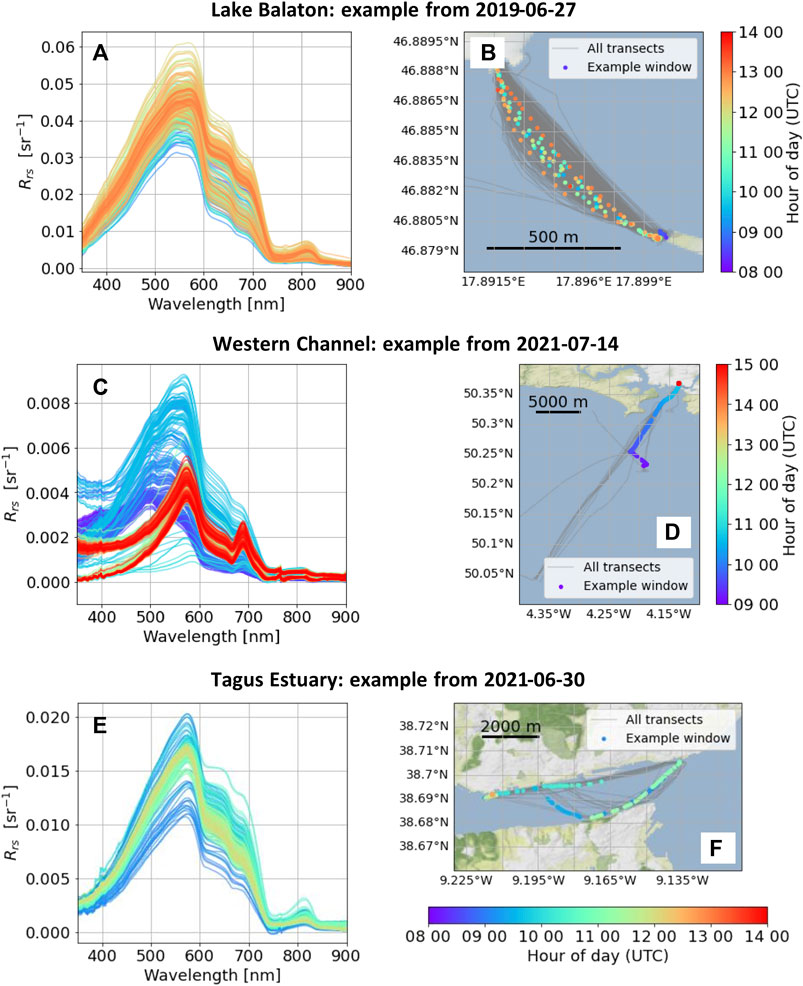
FIGURE 1. Example reflectance (R_rs) spectra and ship transects from each deployment. Top row (A, B) Lake Balaton. Centre row (C, D) Western Channel. Bottom row (E, F) Tagus Estuary. The R_rs spectra correspond to a time window of data as used in the variogram analysis (6 h for Lake Balaton and the Western Channel and 4 h for the Tagus Estuary) centred around noon in the local time zone. The R_rs spectra are referenced to the points and colour bar in the coverage maps.

3.4 Data gridding and selection from time window

Prior to the variogram analsyis (Section 4), the hyperspectral in situ R_rs spectra were downsampled to discrete spectral bands centred on 443, 560, 665, and 783 nm using a Gaussian weighting based on the full width at half maximum of the MSI spectral response function. The band centres correspond to the chlorophyll-a absorption maximum (443 nm), the chlorophyll-a reference/absorption minimum (560 nm), the second chlorophyll-a absorption maximum/suspended sediment band (665 nm) and an NIR band used for atmospheric correction (783 nm). OLCI has similar band centres at 443 nm, 560 nm, 665 nm. R_rs within each spectral band was then resampled to a regular 20 m grid, taking the mean R_rs when there were multiple measurements within each grid cell. The gridding represents a practical lower bound on the length scale for comparisons to be made between in situ and satellite R_rs, and follows how in situ R_rs has been gridded for MSI validation (Warren et al., 2019). The gridding also regularizes the sampling for the variograms as longer time series when the ship is stationary are averaged to a single measurement.

Our variogram analysis considers the spatial dependence of R_rs variability, but neglects (explicit) temporal variation. For each variogram computation, in situ R_rs were selected on a daily basis from a time window centred about 12 noon in the local time zone, allowing ±3 h from noon for the Lake Balaton and Western Channel deployments, and ±2 h for the more dynamic Tagus Estuary. The time window lengths are a trade-off so that data can be adequately sampled to generate the variograms, whilst being sufficiently short to be (broadly) comparable to a satellite match-up window (Section 2.1). The variograms are computed from multiple pairwise in situ measurements, so the associated timescale differs from the single match-up pairs that are used in satellite validation. The distribution of pairwise time separation therefore gives an alternative quantification of the time difference between R_rs measurements within the variogram (Figures 2A–C). The distributions have a strong positive skew and median time separations of 1.29 decimal hours (Lake Balaton), 0.90 decimal hours (Western Channel), 1.05 decimal hours (Tagus Estuary). The Western Channel has the lowest pairwise time separation, as the transects are typically collected over a fraction of the allowed time window (e.g., Figure 1D).

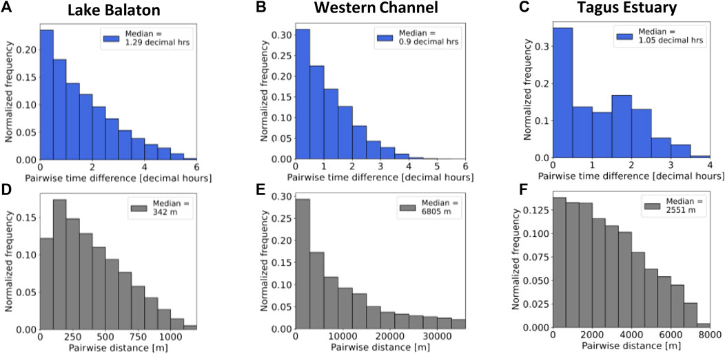
FIGURE 2. Top row (A–C): Normalized frequency distributions of pairwise time separation for each deployment. Bottom row (D–F): Normalized frequency distributions of pairwise point-separation distance for each deployment.

Additionally, the distribution of pairwise point separations, which are an input to the variogram analysis, are shown for each deployment in Figures 2D–F. The maximum point separations are ∼ 1,200 m for Lake Balaton, ∼ 35,000 m for the Western Channel, and ∼ 8,000 m for the Tagus Estuary.

4 Materials and methods

4.1 Overview of variogram analysis

The variogram is a commonly used graphical method to characterize variation in a geographic quantity as a function of the separation distance between measurements, and is described in geostatistics textbooks (e.g., Cressie, 1993) aswell as ocean colour studies (e.g., Glover et al., 2018). The variogram enables partitioning of variance into a structural component that is associated with spatial separation and an intrinsic component not associated with spatial separation. The variogram also enables characterization of the autocorrelation length, which is the characteristic length scale at which a quantity ceases to be spatially correlated with neighbouring observations.

Variogram analysis expresses the semivariance (γ) as a function of separation distance (h), which is also referred to as the lag or ground-sample distance (GSD). For in situ R_rs, computation of the semivariance uses an equation of the form

where R_rs(x_i) is an in situ reflectance observation at geographic location x_i and, N(h) is the total number of measurement pairs at distance h (Glover et al., 2018). γ(h) is computed separately for each spectral band. The summation in Eq. 6 applies across the set of all pairwise point separations, and pivots about each data point in turn, sampling from a circular annulus with thickness δh (the lag bin width). The radial sampling method can be applied to both distributed data (as occurs for the variable paths of the Lake Balaton car ferry, Figure 1A) and purely transect-like data (as is the case for the Western Channel deployment). Eq. 6 assumes that γ(h) depends only on h but not on the spatial location. In other words, γ(h) represents an average quantity computed over the extent of the geographic survey, unless spatial windowing is applied. As it graphs the semivariance, the variogram is sometimes referred to as a semivariogram (Bachmaier and Backes, 2011). Eq. 6 is applied after quality control of R_rs (see Section 3.2). Numerical details on the computation of γ(h) and fitting procedure are provided in Section 4.3.

γ(h) in Eq. 6 can be interpreted as representing the variance in R_rs at separation distance h (refer to Bachmaier and Backes (2011) for an explanation how the formula relates to a conventional expression for the variance). In the context of in situ R_rs, γ(h) has units sr⁻². In satellite validation of R_rs it is preferable to express uncertainty in units of sr⁻¹ (i.e., expressed as a standard deviation of R_rs). We therefore consider graphs of $\sqrt{\gamma (h)}$ which we refer to as the “root-variogram”.

4.2 Interpreting the root-variogram and spatial structure of in situ R_rs

This section describes the features of the root-variogram and how these relate to spatial properties of R_rs. A schematic example from Lake Balaton is shown in Figure 3 for R_rs(560). The root-variogram (Figure 3A) shows empirical computations (points) and fitted curves (solid lines), with the computations and fitting procedure described in Section 4.3. The root-variogram has three fitted parameters: $\sqrt{C_0}$ is the value of $\sqrt{\gamma (h)}$ when h = 0 (with C₀ often referred to as the variogram nugget), $\sqrt{C_{\infty }}$ is the value of $\sqrt{\gamma (h)}$ as h tends to infinity (with C_∞ often referred to as the variogram sill) and L is the autocorrelation length (often referred to as the variogram range). The model fits (Section 4.3) assume a Gaussian semivariance function of the form

where k is a constant. In the data analysis we also consider the root-variogram normalized by the survey mean $(\overline{R_{rs}})$ which we define as $\widetilde{CV}(h)=100\sqrt{\gamma (h)}/{\bar{R}}_{rs}$ due to the analogy with the coefficient of variation. This normalization is done to compare relative variation between spectral bands and deployments, as the R_rs magnitude can vary substantially (Figure 1). Examples of the normalized variogram curves are shown in Figure 3B.

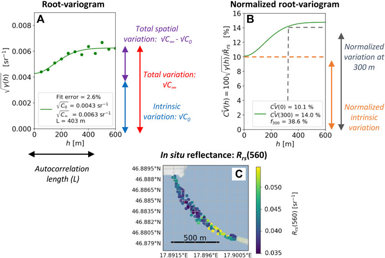
FIGURE 3. Annotated examples of (A) root-variogram, $\sqrt{(\gamma (h))}$, (B) normalized root-variogram $\widetilde{CV}(h)=100\sqrt{\gamma (h)}/{\bar{R}}_{rs}$, (C) corresponding reflectance map for R_rs(560). Panel A shows the three fitted parameters: $\sqrt{C_0}$ (variogram nugget, representing variation in R_rs as h tends to zero), $\sqrt{C_{\infty }}$ (variogram sill, representing variation in R_rs as h tends to infinity), and L (autocorrelation length; the distance R_rs ceases to be spatially autocorrelated), along with the curve fit (mean percentage) error. Panel B shows measures of normalized variation at h = 0 m and h = 300 m that are used in the computation of f₃₀₀, using Eq. 8. The example is from 2019-06-27 and corresponds to the same data as Figures 1A,B.

$\sqrt{C_0}$, $\sqrt{C_{\infty }}$, L and derived parameters relate to the spatial structure of in situ R_rs as follows:

Intrinsic variability represents variation in R_rs that is not due to measurement point separation. In the root-variogram, intrinsic variation is quantified by $\sqrt{C_0}$ (the h = 0 intercept of the fitted curve) and in the normalized root variogram, by $\widetilde{CV}(0)=100\sqrt{C_0}/{\bar{R}}_{rs}$. In the data analysis, we focus on $\widetilde{CV}(0)$ as it provides a relative measure of intrinsic variation between spectral bands and deployments. Intrinsic variability arises from a combination of factors including instrument noise, environmental perturbations, and precision of the R_rs retrieval method (further discussed in Section 6.3).

Spatial variability represents variation in R_rs that occurs due to measurement point separation. The quantity $\sqrt{C_{\infty }}-\sqrt{C_0}$, the amount by which the root-variogram nugget exceeds the root-variogram sill, quantifies the maximum spatial variation in R_rs that occurs due to measurement point separation, and is indicated graphically in Figure 3A. In the data analysis we focus on spatial variability at a length scale representative of a medium resolution sensor pixel (300 m). We do this by quantifying the fraction of variation in R_rs associated with spatial separation at 300 m

where the numerator, $\sqrt{(\gamma (300)}-\sqrt{C_0}$, represents the spatial component of variability at 300 m and the denominator, $\sqrt{\gamma (300)}$, represents the total variation. A way to interpret f₃₀₀ is that it relates to a reduction in spatial discrepancy uncertainty (i.e., reduction of the Δ_s term in Eq. 4) due to sampling across the satellite pixel. Specifically, $\sqrt{\gamma (300)}-\sqrt{C_0}$ represents the additional variation across the pixel that the mobile radiometer samples relative to a fixed platform which samples a single fixed location and $\sqrt{\gamma (300)}$ represents the total variation that measurements from a fixed platform would be subject to. Therefore $f_{300}=(\sqrt{\gamma (300)}-\sqrt{C_0})/\sqrt{\gamma (300)}$ serves as a relative measure of the capacity of the mobile radiometers to sample sub-pixel variability. f₃₀₀ is illustrated graphically in Figure 3B, taking into account that the f₃₀₀ ratio is the same in the normalized plot; i.e., $\left(\sqrt{\widetilde{CV(300)}}-\sqrt{\widetilde{CV(0)}}\right)/\sqrt{\widetilde{CV(300)}}\equiv \left(\sqrt{\gamma (300)}-\sqrt{C_0}\right)/\sqrt{\gamma (300)}$.

Spatial autocorrelation. The autocorrelation length L quantifies the separation distance at which R_rs measurements cease to be spatially correlated with the original location. This is also the distance at which further increasing measurement point separation does not increase the variation in R_rs. In general, the definition of L can vary between variogram models and correspondingly the decay constant k in Eq. 7 can also take different definitions (Mälicke, 2022). Here we set k = 3 which corresponds to the fitted curve reaching ∼ 98% of the difference between the sill value $(\sqrt{C_{\infty }})$ and the nugget value $(\sqrt{C_0})$.

4.3 Computation and fitting of the variograms

Prior to the variogram analysis, geographic coordinates were converted to Universal Transverse Mercator coordinates using the WGS 84 ellipsoid. The variogram computations were performed using the Python geostatistics module (Mälicke 2022) using the inbuilt variogram function to compute γ(h) via Eq. 6. The computations select R_rs data from 12 discretized lag (h) bins. Following recommendations that the maximum lag must be order half the maximum point separation or less (Mälicke, 2022), the maximum possible lag of 600 m was used for Lake Balaton, corresponding to a bin width of δh = 50 m. For the other deployments a maximum lag of 1,500 m was used, corresponding to a bin width of δh = 125 m.

The fitting of Eq. 7 to the empirical variogram, which determines $\sqrt{C_0}$, $\sqrt{C_{\infty }}$ and $L$, used the Levenberg-Marquardt (non-linear least squares) algorithm. The absolute mean percentage error between empirical and fitted variogram curves was used to measure the goodness-of-fit. It was then used as a quality control parameter to filter out poor fits to the Gaussian model, with 10% used as maximum allowed value. In our study the Gaussian model was used as it gave the best overall fit to the data from the conventional choices of variogram model (spherical, Gaussian, exponential). Future studies on different data sets should experiment with different choices of parametric model, or non-parametric approach to extract the variogram parameters. Additionally, we required that at least 60 (Lake Balaton) or 100 (Western Channel, Tagus Estuary) data points were present to generate the variograms. (The number of data points available fluctuates due to the variable ship paths, variable time intervals when the ship is stationary, and R_rs quality control (Section 3.2)).

5 Results

5.1 Variogram structure of in situ R_rs

We first illustrate how the spatial distribution of in situ R_rs relates to variogram structure, and how this can differ for different days within each deployment or between spectral bands. The examples from Lake Balaton (Figure 4) illustrate different degrees of spatial structure within the green band (R_rs(560)). The example in the top row (Figures 4A–C) has significantly more spatial variation than the bottom row (Figures 4D–F) indicated by the steeper curve and the greater difference between $\sqrt{C_{\infty }}$ and $\sqrt{C_0}$ (absolute measure of total spatial variation) and f₃₀₀ (relative measure of spatial variation at 300 m). The differences in variogram structure relate to the R_rs(560) map in the top row having greater spatial coherence than the bottom row. The examples from the Western Channel (Figure 5) are chosen to illustrate subtle differences between the variogram structure for different spectral bands within the same match-up window. Notably, R_rs(560) in the bottom row has a longer autocorrelation length (1,053 m) than R_rs(443) in the bottom row (678 m). The larger autocorrelation length means that spatial variation in R_rs(560) occurs over a longer length scale than R_rs(443), visually corresponding to a smoother spatial gradient in the R_rs(560) map. The examples from the Tagus Estuary (Figure 6) are chosen to illustrate different degrees of intrinsic variation that can occur within each deployment. Specifically, the example in the bottom row has much higher intrinsic variation ($\widetilde{CV}(0)$ = 16.3%) than the top row ($\widetilde{CV}(0)$ = 8.3%).

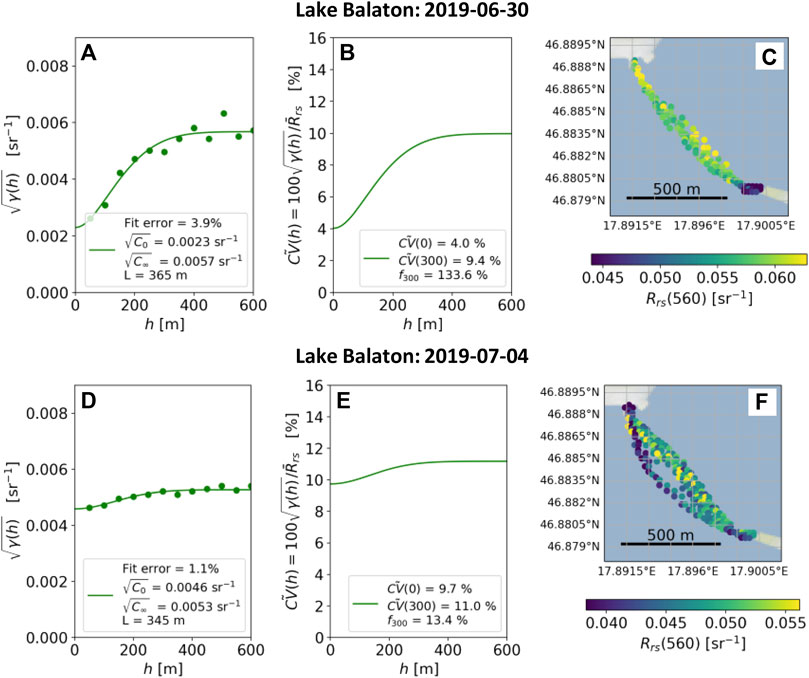
FIGURE 4. Illustrative examples of root-variograms $\sqrt{(\gamma (h))}$ (panels A and D), normalized root-variograms $\widetilde{CV}(h)=100\sqrt{\gamma (h)}/{\bar{R}}_{rs}$ (panels B and E), and corresponding reflectance maps (panels C and F) from the Lake Balaton deployment for R_rs(560). The examples illustrate difference degrees of spatial structure.

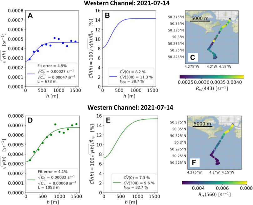
FIGURE 5. Illustrative examples of root-variograms $\sqrt{(\gamma (h))}$ (panels A and D), normalized root-variograms $\widetilde{CV}(h)=100\sqrt{\gamma (h)}/{\bar{R}}_{rs}$ (panels B and E), and corresponding reflectance maps (panels C and F) from the Western Channel deployment for R_rs(443) (top row) and R_rs(560) (bottom row). The examples illustrate subtle differences in the variogram shapes and autocorrelation length between the 443 nm and 560 nm bands. The data in both rows is the same as in Figures 1C,D.

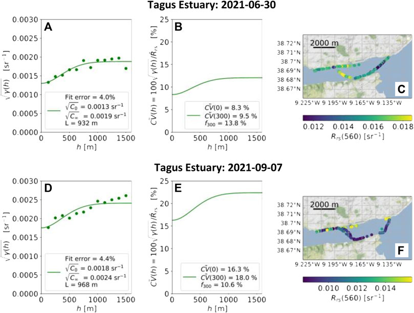
FIGURE 6. Illustrative examples of root-variograms $\sqrt{(\gamma (h))}$ (panels A and D), normalized root-variograms $\widetilde{CV}(h)=100\sqrt{\gamma (h)}/{\bar{R}}_{rs}$ (panels B and E), and corresponding reflectance maps (panels C and F) from the Tagus Estuary deployment for R_rs(560). The examples illustrate differences in intrinsic variation in R_rs. The data in the top row is the same as in Figures 1E,F.

Figures 7, 8 show summaries of root-variograms $(\sqrt{\gamma }(h))$ and normalized root-variograms $(\widetilde{CV}(h)=100\sqrt{\gamma (h)}/{\bar{R}}_{rs})$ across the three deployments in four spectral bands: 443 nm (blue), 560 nm (green), 665 nm (red), 783 nm (NIR). The purpose here is to provide an overall summary, and related variogram statistics are described in Section 5.2. Each individual $\sqrt{\gamma }(h)$ curve represents a theoretical fit to the empirical root variogram. Curves based on the median goodness-of-fit parameters are also shown. The $\sqrt{\gamma }(h)$ curves in Figure 7 illustrate that, for each deployment, the dependence of absolute variation in R_rs scales broadly with the spectral shape and magnitude of the R_rs spectra in Figure 1. Specifically, across the deployments, the values of $\sqrt{\gamma }(h)$ are highest for the 560 nm band, and lowest for the 783 nm band. The $\widetilde{CV}(h)$ curves in Figure 8 illustrate that relative variation in R_rs typically ranges between 5% and 40% for the length scales shown. In reverse of the result in Figure 7 the 665 nm and 783 nm bands have higher relative variability than the shorter wavebands.

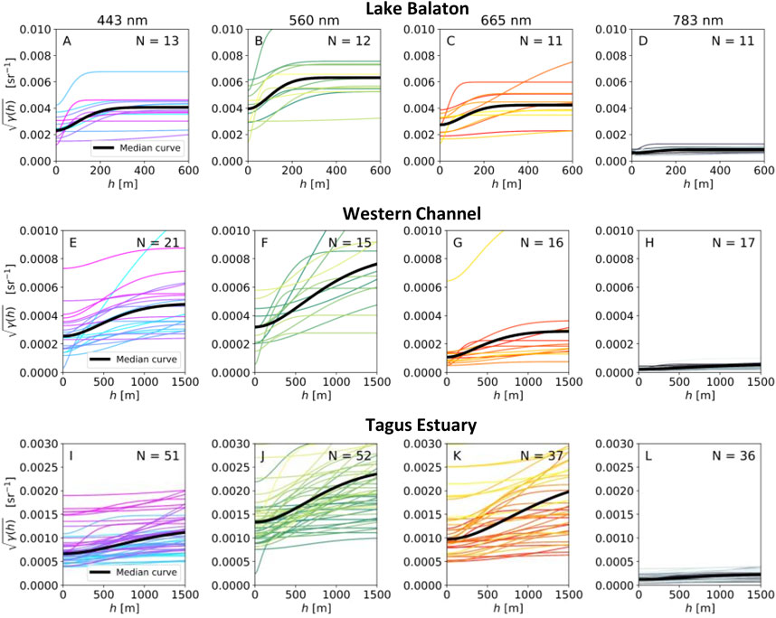
FIGURE 7. Summary of root-variograms $(\sqrt{\gamma }(h))$ in four spectral bands for each window/day of deployment. Top row (A–D): Lake Balaton. Middle row (E–H): Western Channel. Bottom row (I–L) Tagus Estuary. The vertical scale is fixed within a deployment, but differs between different deployments. The horizontal data range is smaller for Lake Balaton than the other deployments. Curves based on median fit parameters are shown. The number of curves (N) varies slightly between spectral bands within each deployment due to quality-control filtering of the variogram fitting (Section 4.3).

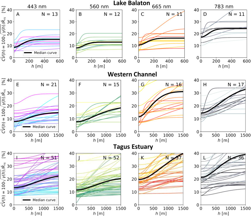
FIGURE 8. Summary of normalized root-variograms $(\widetilde{CV}(h)=100\sqrt{\gamma (h)}/{\bar{R}}_{rs})$ in four spectral bands for each window/day of deployment. Top row (A–D) Lake Balaton. Middle row (E–H) Western Channel. Bottom row (I–L) Tagus Estuary. Curves based on median fit parameters are shown. The number of curves (N) varies slightly between spectral bands within each deployment due to quality-control filtering of the variogram fitting (Section 4.3).

The diversity of curves in each panel in Figures 7, 8 show that a range of variogram structure exists for each deployment and spectral band. However, some clear trends are present. Notably, the variogram curves from Lake Balaton have a markedly different shape than the other deployments, with the sill being reached at shorter length scales than the other deployments (note the different horizontal axis scale in Figure 7). This difference in variogram structure represents that spatial variation in R_rs occurs over a shorter length scale in Lake Balaton than other deployments. Additionally, the Tagus Estuary generally has a greater spread of variogram curves and higher relative variability than the Lake Balaton and Western Channel deployments.

5.2 Variogram statistics for spatial structure of in situ R_rs

Figure 9 shows frequency distributions for $\widetilde{CV}(h)=100\sqrt{C_0}/{\bar{R}}_{rs}$ for each deployment and spectral band. This parameter measures the relative intrinsic variation in R_rs (i.e., percentage variation in R_rs not due to measurement point separation) and corresponds to the distributions of the h = 0 intercepts in Figure 8. Median values of $\widetilde{CV}(0)$ range from 7% to 21% across spectral bands and deployments. Within each deployment, the blue and green bands typically have the lowest variability with the red and NIR bands having the highest variability. Averaged across spectral bands, the Tagus Estuary has significantly higher $\widetilde{CV}(0)$ than the other two deployments (17% compared with 11% and 10% for Lake Balaton and the Western Channel respectively). We note that the results in Figure 9 hold for the normalized variograms. Alternatively, intrinsic variability could be expressed in steradians for absolute values of R_rs (the h = 0 intercepts in Figure 7).

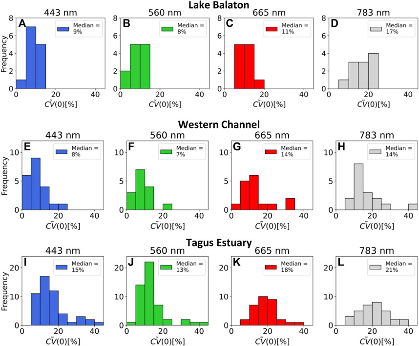
FIGURE 9. Frequency distributions of the intrinsic variation in R_rs as measured by $\widetilde{CV}(0)=100\sqrt{C_0}/{\bar{R}}_{rs}$ where $\sqrt{C_0}=\sqrt{\gamma (0)}$ is the intercept of the root-variogram. Top row (A–D) Lake Balaton. Middle row (E–H) Western Channel. Bottom row (I–L) Tagus Estuary. This parameter represents all variation in R_rs not due to measurement point separation.

Figure 10 shows frequency distributions for f₃₀₀, Eq. 8, for each deployment and spectral band. This parameter represents the fraction of R_rs variability due to measurement point separation at 300 m (chosen due to the pixel size of OLCI). The values of f₃₀₀ are significantly higher for Lake Balaton than the other deployments, with median values $>$ 30% in the blue, green and red bands. The Tagus Estuary has lower values of f₃₀₀ than the other deployments with median values $<$ 10% in all bands. The Western Channel has the greatest difference in f₃₀₀ between spectral bands, with median value 21% for the green band and 7% for the NIR band. The f₃₀₀ distributions are broad and values often greatly exceed the median; e.g., the example in the top row of Figure 4 has f₃₀₀ > 100%, indicating that over half of the variation at 300 m is due to measurement point separation.

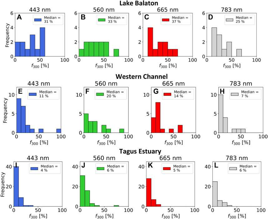
FIGURE 10. Frequency distributions of spatial variation in R_rs as measured by $f_{300}=100\left(\sqrt{(\gamma (300)}-\sqrt{C_0}\right)/\sqrt{\gamma (300)}$. Top row (A–D) Lake Balaton. Middle row (E–H) Western Channel. Bottom row (I–L) Tagus Estuary. This parameter represents the percentage of the variation in R_rs associated with spatial separation at a length scale of 300 m; typical of a medium resolution sensor such as OLCI. Outliers (f₃₀₀ > 100 %) are not shown.

Figure 11 shows frequency distributions for the autocorrelation length, L. Lake Balaton has lower values of L than the other deployments, with median values between 250 and 300 m. The Western Channel has median values of L between 1,000 and 500 m, with the Tagus Estuary between 1,800 and 2,500 m. In all panels the frequency distributions for L are broad, indicating that the spatial autocorrelation structure of in situ R_rs is changeable throughout the timescale of the deployment.

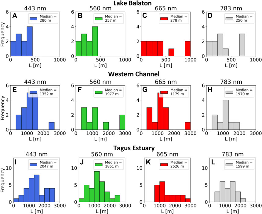
FIGURE 11. Frequency distributions of variogram autocorrelation lengths (L). Top row (A–D) Lake Balaton. Middle row (E–H) Western Channel. Bottom row (I–L) Tagus Estuary. This parameter represents the maximum distance at which in situ R_rs is considered spatially correlated with neighbouring observations. Outliers (L > 1,000 m in the top row and L > 3,000 m in the middle and bottom rows) are not shown.

We note that the results for f₃₀₀ in Figure 10 and for L in Figure 11 hold for both unnormalized $(\sqrt{\gamma (h)})$ and normalized $(\widetilde{CV}(h))$ root-variograms.

6 Discussion

6.1 Comparison with previous variographic analyses of ocean colour and inland water quality

The spatial structure of R_rs (or related ocean colour variables) has been assessed in numerous past studies, based on satellite images (Yoder et al., 1987; Aurin et al., 2013; Glover et al., 2018), airborne (Bissett et al., 2004; Davis et al., 2007; Moses et al., 2016) and shipborne (Moses et al., 2016) radiometric platforms. The key novelty of our study is quantification of the spatial structure of in situ R_rs from autonomous radiometric systems deployed in the context of satellite validation. In coastal regions, reported autocorrelation lengths range from ∼ 1–100 km (Davis et al., 2007; Aurin et al., 2013; Moses et al., 2016), consistent with the Western Channel and Tagus estuary deployments in our study (Figure 11). For example, in near-coastal waters Moses et al. (2016) established that R_rs variability can increase rapidly when measured on scales of 10–100 m (up to a ∼ three-fold increase in the local coefficient of variation from a point measurement) with typical autocorrelation lengths being kilometer-scale. In Monterey Bay, California, Davis et al. (2007) showed autocorrelation lengths to be $>$ 2 km. Aurin et al. (2013) showed that sediment river plumes have autocorrelation lengths which range from ∼ 10–100 km. In the open ocean, spatial autocorrelation can occur over even larger length scales, with Glover et al. (2018) showing autocorrelation lengths to be in the range 50–300 km.

Spatial structure analysis has also been applied to a diversity of chlorophyll measurements (which strongly correlates with R_rs) in inland water bodies. Using a chlorophyll index derived from airborne optical data Hedger et al. (2001) investigated spatial correlation in two Scottish Lochs (Loch Ness, and Loch Awe) reporting autocorrelation lengths between 500 and 1,300 m. Using discrete in situ Chlorophyll-a measurements, Yenilmez et al. (2014) reported autocorrelation length 1,200 m for the Porsuk Dam Reservoir in Turkey, and Anttila et al. (2008) reported autocorrelation lengths of 945 m and 1,357 m in Lake Vesijärvi, Finland. These autocorrelation lengths are slightly higher than the ferry transect we analysed in Lake Balaton (Figures 11A–D) suggesting that ∼ 1 km is a typical length scale of autocorrelation in inland waters.

There are examples of ocean colour variogram structure being more complex than the monotonically increasing Gaussian model used in this study. For example, Aurin et al. (2013) revealed the presence of ‘sub-sills’ (i.e., where the variogram levels out, then rises again), associated with sediment plumes. As we applied a goodness-of-fit filter to the Gaussian model, variograms that deviated significantly from a monotonic increase were filtered out. In comparing variograms between different ocean colour studies, it remains important to note that the transect-like data from shipborne or airborne sampling result in non-uniform spatial sampling, whereas a satellite image will be approximately uniform.

6.2 Opportunities and challenges of using mobile radiometers in satellite validation

Mobile radiometers deployed on ships-of-opportunity enable high-frequency spatial sampling of in situ R_rs in coastal and inland waters. In the context of satellite validation, the obvious advantage to using a mobile system (versus a fixed-platform deployment) is that it enables sampling of variation in in situ R_rs within a satellite pixel and across optical gradients. Quantifying within-pixel variability is important as nearshore waters are dynamic across short spatiotemporal scales which means that selecting spatially homogeneous sites for satellite validation is not always possible or desirable. Sampling in situ R_rs across optical gradients is particularly desirable to validate the response of algorithms over a wide biogeochemical concentration range. A specific challenge in improving validation practice from moving platforms is to account for spatial autocorrelation when selecting in situ data for match-ups with the same satellite image. In a wider context of data integration, it is also desirable to relate point-like in situ reflectance data to optical image data taken at different scales; ranging from drone flight imagery to high and moderate resolution imagery from satellites.

To quantify pixel-scale variation in in situ R_rs within our 4 or 6 h time windows, we introduced the parameter f₃₀₀ which quantifies the percentage of in situ R_rs variation due to spatial separation at 300 m (representative of the medium resolution OLCI sensor). The advantage of using a mobile radiometric system to sample sub pixel variation was particularly clear for the Lake Balaton deployment, where f₃₀₀ was greater than 30% across all spectral bands (median values in Figure 10). This was likely because spatial coherence of in situ R_rs was preserved throughout the time window. On the other hand, the Western Channel and Tagus Estuary deployments are more dynamic systems, which likely results in lower spatial coherence and lower values of f₃₀₀. In tidal systems, fixed-monitoring stations are also able to sample spatial variation due to the flow of water (Salama et al., 2022), representing an alternative strategy to reduce uncertainty in a validation analysis.

Ultimately, it is the average value of in situ R_rs sampled within the extent of a satellite pixel that is compared to the satellite observation, and numerically relates to Δ_s in Eq. 4. The spatial sampling of the mobile radiometer will reduce the standard error on the pixel mean by a factor proportional to $(\sqrt{\gamma (300)}-\sqrt{C_0})/\sqrt{N}$ where N is the number of spatial locations within the pixel that are sampled, and ultimately determined by platform speed and sensor sampling rate. This means that, for mobile radiometric systems, it is valuable to retain all observations sampled along a transect prior to any data reduction by aggregation or selection, and even on-board analysis of transect observations could be considered. In the context of using in situ data for sub-pixel averaging, interpolation across the pixel (e.g., Kriging, based on the variogram structure) could be used to get a more spatially representative average to compare with the satellite image.

In general, accounting for the spatial autocorrelation of in situ R_rs in validation of remotely-sensed reflectance becomes more important as the resolution of the satellite sensor increases. This is because neighbouring measurements become more likely to be located in adjacent pixels, rather than being averaged within the same pixel. If multiple match-up pairs are used from the same image, a simple approach to account for spatial autocorrelation is to downsample the match-up pairs, based on the autocorrelation length, L. Using Lake Balaton as an example, with a median value of L between 250 and 300 m, match-up pairs for high resolution sensors such as MSI could be downsampled to a 300 m spacing, thus reducing the effect of spatial autocorrelation, and thus providing a suitable number of match-up pairs. As the Lake Balaton autocorrelation lengths were generally comparable to the OLCI pixel scale downsampling is not necessary for OLCI match-up pairs from this area of Lake Balaton. For the other two deployments, downsampling match-up pairs to a separation distance of ∼ 2–3 km would be effective to reduce the effects of spatial autocorrelation.

Due to the breadth of the L distributions in Figure 11, and the range of reported water autocorrelation lengths in Section 6.1, it is desirable that downsampling uses the specific variogram on the day of data collection to set the separation distance for the downsampling of in situ R_rs. However, recognising that coincidence of remote and in situ observations is a rarity, as a rule of thumb ∼ 1 km is likely to be an appropriate separation distance for inland waters, with 1 km a minimum distance for coastal waters, being aware that sediment features may have much longer scales of autocorrelation (Aurin et al., 2013). Additionally, spatial structure analysis could be applied to climatologically-averaged ocean colour products to produce a map representing a first-order approximation of spatial autocorrrelation. Downsampling represents just one approach to account for spatial autocorrelation in validation statistics. Alternatively, validation statistics could be modified for spatial autocorrelation; for example, spatially-weighted regression methods (Anselinm and Bera, 1998).

As chlorophyll-a concentration often controls the majority of the variability in R_rs, it typically results in a high degree of co-variance between spectral bands (e.g., Cael et al., 2023). This is reflected in the variogram statistics in Section 5.2 which show similarity between spectral bands, although band differences can exist (e.g., as shown for the Western Channel in Figures 10, 11) when there is variation in the spectral shape of R_rs (Figure 1C). We anticipate that variogram statistics could have the most pronounced differences between spectral bands in optically complex waters, where higher concentrations of suspended sediment and CDOM are present. We therefore recommend continued evaluation of variogram statistics across reflectance bands in coastal and inland waters, until more general conclusions can be drawn on differences between spectral bands.

6.3 Relationship between intrinsic variation and uncertainty of R_rs

In this study, we used the metric $\widetilde{CV}(0)=100\sqrt{C_0}/{\bar{R}}_{rs}$ to characterize intrinsic variation in in situ R_rs; i.e., all variation not due to measurement point separation (see Figure 9 for a summary). This quantity has parallels with the variation in in situ R_rs that would be measured at a fixed-location, e.g., using a coefficient of variation metric applied to time series of R_rs in a local time window (Groetsch et al., 2020), with $\widetilde{CV}(0)$ representing a survey-wide average of variability at a fixed location. This interpretation is supported by the values of $\widetilde{CV}(0)$ in Figure 9 being broadly comparable with fixed-location variability from the same radiometric system (Jordan et al., 2022), where typical coefficient of variation values were ∼ 5%–20% across different measurement conditions.

Measures of R_rs variability provide only a proxy for uncertainty. Formal uncertainty assessment from fiducial reference measurements refers to a component-by-component propagation of sources of uncertainty, traceable to metrology standards (Ruddick et al., 2019; Banks et al., 2020). Individual sources of uncertainty include radiometric calibration, sensor characteristics (e.g., straylight, non-linearity, thermal response), and the uncertainty of the R_rs estimation method, which is impacted by environmental conditions: i.e., cloud cover and windspeed (surface roughness). Environmental sources of uncertainty are typically half of the total uncertainty budget (Lin et al., 2022), with higher windspeeds and scattered cloud leading to higher uncertainties. Variable environmental conditions are therefore likely to be a dominant factor influencing the spread of $\widetilde{CV}(0)$ in Figure 9. As co-located wind data were not available to do this in the current study, investigating environmental controls on variogram structure (including strictness of quality control) is an area for future investigation.

6.4 Limitations of variogram analysis and future work

Due to computing the variogram over a 4 or 6 h time window, there are temporal sources of variation that are present in the analysis. These include variation in R_rs due to changing solar zenith and relative azimuth (Mobley, 1999), as well as natural temporal fluctuations in water constituent concentrations. Casting the analysis in terms of the normalized water leaving radiance, which adjusts for R_rs variable zenith angle and atmospheric attenuation (Gordon and Wang, 1994), would give a more accurate picture of how the water properties vary spatially. Additionally, the variogram structure will be impacted by temporal variation. For example, in the Tagus Estuary deployment, the relatively high variation in in situ R_rs at shorter length scales (Figure 9) is hypothesised to be partially influenced by the ship revisiting a location where R_rs changed temporally due to tidal influence (see neighbouring transects collected at different times in Figure 1F). Temporal R_rs differences between neighbouring transects is also likely to have an impact on the spatial structure analysis from Lake Balaton.

An important caveat to the variogram analysis is that the ship transects do not uniformly sample across the survey area, or each pixel. Therefore, the variogram structure is anticipated to be specific to the path of the ship within each deployments, and is likely to be very different for alternative ship paths in the same water body. Additionally, due to the quality control of in situ R_rs (Section 3.2) the effective temporal sampling frequency is also subject to change, because not all observations taken along a transect are suitable to derive estimates of R_rs.

A future research direction is to extend the “static” variogram analysis to the temporal dimension, and hence enable spatial and temporal autocorrelation to be considered in a unified way. It is likely this will require the data sampling strategy to be developed around the analysis method; i.e., obtaining repeat in situ measurements at a set of fixed locations that can be used to robustly window the variograms. Alternatively, a sequence of images from geostationary satellites which have hourly revisit times (e.g., Choi et al., 2012) could be used to gain insight.

7 Summary and conclusion

This study quantified the spatial structure of in situ R_rs from mobile radiometers deployed in coastal and inland water bodies. The overarching aim was to inform how spatial statistics can be used to aid in satellite validation practice where ship-transect data is used. A first focus was quantifying how mobile radiometers can reduce variability via sub-pixel sampling and a second focus was quantifying spatial autocorrelation, and thereby informing in situ data selection for match-up analysis.

There were pronounced differences in spatial structure between the deployments, within each deployment, as well as more subtle differences between spectral bands. At a 300 m length scale (typical pixel size of a medium resolution ocean colour satellite sensor) we showed that typically 5%–35% of the total variation in in situ R_rs was due to the spatial separation of measurements. For validation of medium-resolution sensors, mobile radiometers therefore provide a distinct advantage in generating more spatially representative data than a fixed platform, reducing the contribution of in situ variability in the validation process. The autocorrelation length, which informs an ideal minimum separation distance for in situ R_rs in validation, ranged from ∼ 100–1,000 m. Consequently, validation of high-resolution sensors (sub 100 m pixel size) requires either downsampling of in situ data to ensure spatial independence or for validation statistics to take spatial autocorrelation into account.

In the future, we anticipate that spatial statistics will become increasingly important for both validation and data integration of aquatic reflectance across multiple sensor systems, including spaceborne, shipborne, airborne, and ground-based platforms.

Data availability statement

The datasets presented in this study can be found in online repositories. The names of the repository/repositories and accession number(s) can be found below: https://pypi.org/project/monda/; https://github.com/tjor/SR_variograms.

Author contributions

TJ, SS, and NS contributed to conception and design of the study. TJ led the data analysis with contributions from SS and NS. SS, VM-V, GS, and FI designed the field deployments and collected data. TJ led the writing of the manuscript with contributions from all authors. SS obtained the primary funding and administered the project. All authors contributed to the article and approved the submitted version.

Funding

This project received primary funding from the European Union’s Horizon 2020 research and innovation programme under grant agreement No 776480 (MONOCLE: Multiscale Observation Networks for Optical monitoring of Coastal waters, Lakes and Estuaries), https://monocle-h2020.eu. TJ and VM-V were partially supported by Hyperspectral Bio-Optical Observations Sailing on Tara (HyperBOOST) (ESA contract number: 4000135756/21/I-EF). GS and FI acknowledge funding from from Horizon 2020 grant agreement No 870349 (CERTO: Copernicus Evolution: Research for harmonised and Transitional water Observation). TJ was partially funded by NERC through its Earth Observation Data Acquisition and Analysis Service (NEODAAS), award number NE/S013377/1.

Acknowledgments

We would like to thank our reviewers whose thorough and constructive comments greatly improved our publication.

Conflict of interest

The authors declare that the research was conducted in the absence of any commercial or financial relationships that could be construed as a potential conflict of interest.

Publisher’s note

All claims expressed in this article are solely those of the authors and do not necessarily represent those of their affiliated organizations, or those of the publisher, the editors and the reviewers. Any product that may be evaluated in this article, or claim that may be made by its manufacturer, is not guaranteed or endorsed by the publisher.

References

Albert, A., and Mobley, C. (2003). An analytical model for subsurface irradiance and remote sensing reflectance in deep and shallow case-2 waters. Opt. Express 11, 2873–2890. doi:10.1364/OE.11.002873
Anselinm, L., and Bera, A. K. (1998). Spatial dependence in linear regression models with an introduction to spatial econometrics. CRC Press, 237–290. chap. 7. doi:10.1201/9781482269901-36
Anttila, S., Kairesalo, T., and Pellikka, P. (2008). A feasible method to assess inaccuracy caused by patchiness in water quality monitoring. Environ. Monit. Assess. 142, 11–22. doi:10.1007/s10661-007-9904-y
Aurin, D., Mannino, A., and Franz, B. (2013). Spatially resolving ocean color and sediment dispersion in river plumes, coastal systems, and continental shelf waters. Remote Sens. Environ. 137, 212–225. doi:10.1016/j.rse.2013.06.018
Bachmaier, M., and Backes, M. (2011). Variogram or semivariogram? Variance or semivariance? Allan variance or introducing a new term? Math. Geosci. 43, 735–740. doi:10.1007/s11004-011-9348-3
Bailey, S. W., and Werdell, P. J. (2006). A multi-sensor approach for the on-orbit validation of ocean color satellite data products. Remote Sens. Environ. 102, 12–23. doi:10.1016/j.rse.2006.01.015
Banks, A. C., Vendt, R., Alikas, K., Bialek, A., Kuusk, J., Lerebourg, C., et al. (2020). Fiducial reference measurements for satellite ocean colour (FRM4SOC). Remote Sens. 12, 1322. doi:10.3390/rs12081322
Barnes, B. B., Cannizzaro, J., English, D., and Hu, C. (2019). Validation of VIIRS and MODIS reflectance data in coastal and oceanic waters: an assessment of methods. Remote Sens. Environ. 220, 110–123. doi:10.1016/J.RSE.2018.10.034
Bissett, W. P., Arnone, R. A., Davis, C. O., Dickey, T. D., Dye, D., Kohler, D. D., et al. (2004). From meters to kilometers: a look at ocean-color scales of variability, spatial coherence, and the need for fine-scale remote sensing in coastal ocean optics. Oceanography 17 (2), 32–43. doi:10.5670/oceanog.2004.45
Brewin, R. J., Dall’Olmo, G., Pardo, S., van Dongen-Vogels, V., and Boss, E. S. (2016). Underway spectrophotometry along the atlantic meridional transect reveals high performance in satellite chlorophyll retrievals. Remote Sens. Environ. 183, 82–97. doi:10.1016/j.rse.2016.05.005
Bulgarelli, B., Kiselev, V., and Zibordi, G. (2014). Simulation and analysis of adjacency effects in coastal waters: a case study. Appl. Opt. 53, 1523–1545. doi:10.1364/AO.53.001523
Cael, B. B., Bisson, K., Boss, E., and Erickson, Z. K. (2023). How many independent quantities can be extracted from ocean color? Limnol. Oceanogr. Lett. 8, 603–610. doi:10.1002/lol2.10319
Choi, J.-K., Park, Y. J., Ahn, J. H., Lim, H.-S., Eom, J., and Ryu, J.-H. (2012). Goci, the world’s first geostationary ocean color observation satellite, for the monitoring of temporal variability in coastal water turbidity. J. Geophys. Res. Oceans 117. doi:10.1029/2012JC008046
Concha, J. A., Bracaglia, M., and Brando, V. E. (2021). Assessing the influence of different validation protocols on ocean colour match-up analyses. Remote Sens. Environ. 259, 112415. doi:10.1016/j.rse.2021.112415
Cressie, N. A. C. (1993). Statistics for spatial data. Revised Edition. John Wiley and Sons, 27–104. chap. 2. doi:10.1002/9781119115151
Davis, C. O., Kavanaugh, M., Letelier, R., Bissett, W. P., and Kohler, D. (2007). “Spatial and spectral resolution considerations for imaging coastal waters,” in Coastal Ocean remote sensing. Editors R. J. Frouin, and Z. Lee (International Society for Optics and Photonics), 6680, 196–207. doi:10.1117/12.734288
Glover, D. M., Doney, S. C., Oestreich, W. K., and Tullo, A. W. (2018). Geostatistical analysis of mesoscale spatial variability and error in seaWiFS and MODIS/aqua global ocean color data. J. Geophys. Res. Oceans 123, 22–39. doi:10.1002/2017JC013023
Gordon, H. R., and Wang, M. (1994). Retrieval of water-leaving radiance and aerosol optical thickness over the oceans with seawifs: a preliminary algorithm. Appl. Opt. 33, 443–452. doi:10.1364/AO.33.000443
Gregg, W. W., and Carder, K. L. (1990). A simple spectral solar irradiance model for cloudless maritime atmospheres. Limnol. Oceanogr. 35, 1657–1675. doi:10.4319/lo.1990.35.8.1657
Groetsch, P. M. M., Foster, R., and Gilerson, A. (2020). Exploring the limits for sky and sun glint correction of hyperspectral above-surface reflectance observations. Appl. Opt. 59, 2942–2954. doi:10.1364/AO.385853
Groetsch, P. M. M., Gege, P., Simis, S. G. H., Eleveld, M. A., and Peters, S. W. M. (2017). Validation of a spectral correction procedure for sun and sky reflections in above-water reflectance measurements. Opt. Express 25, A742–A761. doi:10.1364/OE.25.00A742
Groom, S., Sathyendranath, S., Ban, Y., Bernard, S., Brewin, R., Brotas, V., et al. (2019). Satellite ocean colour: current status and future perspective. Front. Mar. Sci. 6, 1–30. doi:10.3389/fmars.2019.00485
Hedger, R. D., Atkinson, P. M., and Malthus, T. J. (2001). Optimizing sampling strategies for estimating mean water quality in lakes using geostatistical techniques with remote sensing. Lakes Reservoirs Sci. Policy Manag. Sustain. Use 6, 279–288. doi:10.1046/j.1440-1770.2001.00159.x
Ilori, C. O., Pahlevan, N., and Knudby, A. (2019). Analyzing performances of different atmospheric correction techniques for landsat 8: application for coastal remote sensing. Remote Sens. 11, 469. doi:10.3390/rs11040469
IOCCG (2019). Uncertainties in ocean colour remote sensing. Int. Ocean. Colour. Coord. Group (IOCCG) 18. doi:10.25607/OBP-696
Jordan, T. M., Simis, S. G. H., Grötsch, P. M. M., and Wood, J. (2022). Incorporating a hyperspectral direct-diffuse pyranometer in an above-water reflectance algorithm. Remote Sens. 14, 2491. doi:10.3390/rs14102491
Justice, C., Belward, A., Morisette, J., Lewis, P., Privette, J., and Baret, F. (2000). Developments in the ’validation’ of satellite sensor products for the study of the land surface. Int. J. Remote Sens. 21, 3383–3390. doi:10.1080/014311600750020000
Kutser, T. (2012). The possibility of using the landsat image archive for monitoring long time trends in coloured dissolved organic matter concentration in lake waters. Remote Sens. Environ. 123, 334–338. doi:10.1016/j.rse.2012.04.004
Lee, Z., Hu, C., Arnone, R., and Liu, Z. (2012). Impact of sub-pixel variations on ocean color remote sensing products. Opt. Express 20, 20844–20854. doi:10.1364/OE.20.020844
Lehmann, G., Pahlevan, N., Alikas, K., Conroy, T., and Anstee, J. (2023). Gloria - a globally representative hyperspectral in situ dataset for optical sensing of water quality. Sci. Data 10, 100. doi:10.1038/s41597-023-01973-y
Lin, J., Dall’Olmo, G., Tilstone, G. H., Brewin, R. J. W., Vabson, V., Ansko, I., et al. (2022). Derivation of uncertainty budgets for continuous above-water radiometric measurements along an atlantic meridional transect. Opt. Express 30, 45648–45675. doi:10.1364/OE.470994
Loew, A., Bell, W., Brocca, L., Bulgin, C. E., Burdanowitz, J., Calbet, X., et al. (2017). Validation practices for satellite-based earth observation data across communities. Rev. Geophys. 55, 779–817. doi:10.1002/2017RG000562
Mälicke, M. (2022). Scikit-gstat 1.0: a scipy-flavored geostatistical variogram estimation toolbox written in python. Geosci. Model. Dev. 15, 2505–2532. doi:10.5194/gmd-15-2505-2022
Martinez-Vicente, V., Simis, S. G. H., Alegre, R., Land, S., and Groom, P. E. (2013). Above-water reflectance for the evaluation of adjacency effects in earth observation data: initial results and methods comparison for near-coastal waters in the western channel, UK. J. Euro. Opt. Soc. 8, 13060. doi:10.2971/jeos.2013.13060
Mobley, C. D. (1999). Estimation of the remote-sensing reflectance from above-surface measurements. Appl. Opt. 38, 7442–7455. doi:10.1364/AO.38.007442
Montes, M., Pahlevan, N., Giles, D. M., Roger, J.-C., Zhai, P.-w., Smith, B., et al. (2022). Augmenting heritage ocean-color aerosol models for enhanced remote sensing of inland and nearshore coastal waters. Front. Remote Sens. 3. doi:10.3389/frsen.2022.860816
Moses, W. J., Ackleson, S. G., Hair, J. W., Hostetler, C. A., and Miller, W. D. (2016). Spatial scales of optical variability in the coastal ocean: implications for remote sensing and in situ sampling. J. Geophys. Res. Oceans 121, 4194–4208. doi:10.1002/2016JC011767
Otterman, J., and Fraser, R. S. (1979). Adjacency effects on imaging by surface reflection and atmospheric scattering: cross radiance to zenith. Appl. Opt. 18, 2852–2860. doi:10.1364/AO.18.002852
Pahlevan, N., Mangin, A., Balasubramanian, S. V., Smith, B., Alikas, K., Arai, K., et al. (2021). Acix-aqua: a global assessment of atmospheric correction methods for landsat-8 and sentinel-2 over lakes, rivers, and coastal waters. Remote Sens. Environ. 258, 112366. doi:10.1016/j.rse.2021.112366
Pitarch, J., Talone, M., Zibordi, G., and Groetsch, P. (2020). Determination of the remote-sensing reflectance from above-water measurements with the 3c model: a further assessment. Opt. Express 28, 15885–15906. doi:10.1364/OE.388683
Qin, P., Simis, S. G., and Tilstone, G. H. (2017). Radiometric validation of atmospheric correction for meris in the baltic sea based on continuous observations from ships and aeronet-oc. Remote Sens. Environ. 200, 263–280. doi:10.1016/j.rse.2017.08.024
Román, M. O., Schaaf, C. B., Woodcock, C. E., Strahler, A. H., Yang, X., Braswell, R. H., et al. (2009). The MODIS (collection V005) BRDF/albedo product: assessment of spatial representativeness over forested landscapes. Remote Sens. Environ. 113, 2476–2498. doi:10.1016/j.rse.2009.07.009
Ruddick, K. G., Voss, K., Boss, E., Castagna, A., Frouin, R., Gilerson, A., et al. (2019). A review of protocols for fiducial reference measurements of water-leaving radiance for validation of satellite remote-sensing data over water. Remote Sens. 11, 2198. doi:10.3390/rs11192198
Ryan, J. C., Hubbard, A., Irvine-Fynn, T. D., Doyle, S. H., Cook, J. M., Stibal, M., et al. (2017). How robust are in situ observations for validating satellite-derived albedo over the dark zone of the Greenland ice sheet? Geophys. Res. Lett. 44, 6218–6225. doi:10.1002/2017GL073661
Salama, M. S., Spaias, L., Poser, K., Peters, S., and Laanen, M. (2022). Validation of sentinel-2 (MSI) and sentinel-3 (OLCI) water quality products in turbid estuaries using fixed monitoring stations. Front. Remote Sens. 2. doi:10.3389/frsen.2021.808287
Salama, M. S., and Stein, A. (2009). Error decomposition and estimation of inherent optical properties. Appl. Opt. 48, 4947–4962. doi:10.1364/AO.48.004947
Salama, M. S., and Su, Z. (2011). Resolving the subscale spatial variability of apparent and inherent optical properties in ocean color match-up sites. IEEE Trans. Geoscience Remote Sens. 49, 2612–2622. doi:10.1109/TGRS.2011.2104966
Siegel, D. A., Wang, M., Maritorena, S., and Robinson, W. (2000). Atmospheric correction of satellite ocean color imagery: the black pixel assumption. Appl. Opt. 39, 3582–3591. doi:10.1364/AO.39.003582
Simis, S., Jackson, T., Jordan, T., Peters, S., and Ghebrehiwot, S. (2022). Monda: monocle data analysis python package: so-rad. Available at: https://github.com/monocle-h2020/MONDA.
Simis, S. G. H., and Olsson, J. (2013). Unattended processing of shipborne hyperspectral reflectance measurements. Remote Sens. Environ. 135, 202–212. doi:10.1016/j.rse.2013.04.001
Spyrakos, E., O’Donnell, R., Hunter, P. D., Miller, C., Scott, M., Simis, S. G. H., et al. (2018). Optical types of inland and coastal waters. Limnol. Oceanogr. 63, 846–870. doi:10.1002/lno.10674
Wang, M., Son, S., and Shi, W. (2009). Evaluation of MODIS SWIR and NIR-SWIR atmospheric correction algorithms using seabass data. Remote Sens. Environ. 113, 635–644. doi:10.1016/j.rse.2008.11.005
Warren, M. A., Simis, S. G. H., Martinez-Vicente, V., Poser, K., Bresciani, M., Alikas, K., et al. (2019). Assessment of atmospheric correction algorithms for the sentinel-2a multispectral imager over coastal and inland waters. Remote Sens. Environ. 225, 267–289. doi:10.1016/j.rse.2019.03.018
Wright, A., and Simis, S. G. H. (2021). Construction of the solar-tracking radiometry platform (so-rad). doi:10.5281/zenodo.4485805
Yenilmez, F., Düzgün, S., and Aksoy, A. (2014). An evaluation of potential sampling locations in a reservoir with emphasis on conserved spatial correlation structure. Environ. Monit. Assess. 187, 4216. doi:10.1007/s10661-014-4216-5
Yoder, J. A., McClain, C. R., Blanton, J. O., and Oeymay, L.-Y. (1987). Spatial scales in czcs-chlorophyll imagery of the southeastern u.s. continental shelf. Limnol. Oceanogr. 32, 929–941. doi:10.4319/lo.1987.32.4.0929
Zibordi, G., Kwiatkowska, E., Mélin, F., Talone, M., Cazzaniga, I., Dessailly, D., et al. (2022). Assessment of OLCI-A and OLCI-B radiometric data products across european seas. Remote Sens. Environ. 272, 112911. doi:10.1016/j.rse.2022.112911
Keywords: satellite validation, optical radiometry, above-water reflectance, autonomous monitoring, variogram, spatial structure, water quality
Citation: Jordan TM, Simis SGH, Selmes N, Sent G, Ienna F and Martinez-Vicente V (2023) Spatial structure of in situ reflectance in coastal and inland waters: implications for satellite validation. Front. Remote Sens. 4:1249521. doi: 10.3389/frsen.2023.1249521
Received: 28 June 2023; Accepted: 20 October 2023;
Published: 09 November 2023.
Edited by:
Kevin Ruddick, Royal Belgian Institute of Natural Sciences, BelgiumReviewed by:
Juan Ignacio Gossn, European Organisation for the Exploitation of Meteorological Satellites, GermanyTim J. Malthus, Oceans and Atmosphere (CSIRO), Australia
Susanne Elizabeth Craig, National Aeronautics and Space Administration, United States
Copyright © 2023 Jordan, Simis, Selmes, Sent, Ienna and Martinez-Vicente. This is an open-access article distributed under the terms of the Creative Commons Attribution License (CC BY). The use, distribution or reproduction in other forums is permitted, provided the original author(s) and the copyright owner(s) are credited and that the original publication in this journal is cited, in accordance with accepted academic practice. No use, distribution or reproduction is permitted which does not comply with these terms.
*Correspondence: Thomas M. Jordan, tjor@pml.ac.uk