Sampling strategies for the Herman–Kluk propagator of the wavefunction

Kröninger, Fabian; Lasser, Caroline; Vaníček, Jiří J. L.

doi:10.3389/fphy.2023.1106324

ORIGINAL RESEARCH article

Front. Phys., 23 March 2023
Sec. Chemical Physics and Physical Chemistry
Volume 11 - 2023 | https://doi.org/10.3389/fphy.2023.1106324

Sampling strategies for the Herman–Kluk propagator of the wavefunction

Fabian Kröninger ¹* www.frontiersin.org

Caroline Lasser²*

Jiří J. L. Vaníček ¹*

¹ Laboratory of Theoretical Physical Chemistry, Institut des Sciences et Ingénierie Chimiques, Ecole Polytechnique Fédérale de Lausanne (EPFL), Lausanne, Switzerland
² Zentrum Mathematik, Technische Universität München, Munich, Germany

When the semiclassical Herman–Kluk propagator is used for evaluating quantum-mechanical observables or time-correlation functions, the initial conditions for the guiding trajectories are typically sampled from the Husimi density. Here, we employ this propagator to evolve the wavefunction itself. We investigate two grid-free strategies for the initial sampling of the Herman–Kluk propagator applied to the wavefunction and validate the resulting time-dependent wavefunctions evolved in harmonic and anharmonic potentials. In particular, we consider Monte Carlo quadratures based either on the initial Husimi density or on its square root as possible and most natural sampling densities. We prove analytical convergence error estimates and validate them with numerical experiments on the harmonic oscillator and on a series of Morse potentials with increasing anharmonicity. In all cases, sampling from the square root of Husimi density leads to faster convergence of the wavefunction.

1 Introduction

Semiclassical initial value representation techniques [1, 2] have evolved into useful tools for calculations of the dynamics of atoms and molecules [3]. Frozen Gaussians and their superposition were introduced by Heller in 1981 [4] as an extension to the thawed Gaussian approximation [5] in order to capture non-linear spreading of the wavepackets. Herman and Kluk justified the frozen-Gaussian ansatz and introduced an improved approximation [6–8], now known as the Herman–Kluk propagator, which contains an additional prefactor that rigorously compensates for the fixed width of these frozen Gaussians and ensures unitarity of the time evolution in the stationary-phase limit [7]. The Herman–Kluk approximation keeps the trajectories of the individual Gaussians uncoupled, which sets it apart from the more accurate, but computationally more demanding approaches like the coupled coherent states [9] or the variational multi-configurational Gaussian method [10].

In the spirit of the semiclassical initial value representation, the Herman–Kluk propagator avoids the root search problem [2, 11]. Because of its high accuracy, this propagator belongs among the most successful semiclassical approximations [12–18] and has been derived in many different ways [9, 19–22]. There are observables, such as low-resolution vibronic spectra in mildly anharmonic systems, which can be well described by the more efficient thawed Gaussian approximation [23, 24] and other single-trajectory methods [25–30]. In chaotic and other systems, however, increased anharmonicity leads to wavepacket splitting and non-trivial interference effects. In such situations, the single-trajectory methods break down, whereas the Herman–Kluk propagator often remains accurate and, at the least, provides a qualitatively correct insight (see, e.g., Figure 1). However, in its basic form, the Herman–Kluk propagator cannot describe non-adiabatic dynamics and quantum tunneling. To overcome this limitation, various extensions have been developed: For example, surface hopping Herman–Kluk initial value representation [31, 32] captures non-adiabatic dynamics, whereas higher-order semiclassical corrections to the Herman–Kluk propagator [33, 34] incorporate nuclear tunneling.

FIGURE 1

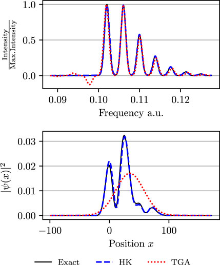
FIGURE 1. Upper panel: Spectra of a Morse potential evaluated using the exact quantum dynamics, Herman–Kluk (HK) propagator, and thawed Gaussian approximation (TGA). Both approximations yield accurate results. Lower panel: Position density at time t ≈ 392 fs propagated in the same Morse potential. In contrast to the Herman–Kluk propagator, the thawed Gaussian approximation does not capture interference between faster and slower components of the wavepacket. For more details, see the last paragraph of Section 4.

The multi-trajectory nature of the Herman–Kluk propagator is not only its advantage, but also its bottleneck. In particular, converged computations might require an extremely large number of trajectories. For this reason, several groups designed various methods, whose goal is reducing the number of trajectories required by the Herman–Kluk propagator. These include, e.g., Filinov filtering [13, 35–37], time-averaging [38–41], semiclassical interaction picture [42, 43], multiple-coherent states [44], hybrid dynamics [45–47], mixed quantum-semiclassical dynamics [48–50], and many others, which achieve the reduction in the number of trajectories by applying one of several possible further approximations.

Yet, the number of guiding trajectories can already be significantly reduced simply by choosing the sampling density of the initial conditions wisely. Although the acceleration of the convergence may be smaller than with the previously mentioned approximate methods, the advantage of this “purely numerical” approach based on improved exact sampling of the unaltered Herman–Kluk initial value representation is that the converged results agree exactly with the converged results of the original Herman–Kluk propagator. For this reason, an early numerical study [8] of the Herman–Kluk wavefunction employed the square root of the Husimi distribution as the sampling density of the initial state, whereas most calculations of observables, time-correlation functions, and wavepacket autocorrelation functions, i.e., quantities quadratic in the wavefunction, correctly employ sampling from the Husimi density [2, 51]. In contrast to observables and correlation functions, the Herman–Kluk wavefunction itself has not been studied much since the early papers [6, 8] and rigorous numerical analysis has been presented only recently [52, 53]. However, the choice of the optimal sampling density for the Herman–Kluk wavefunction itself has not been analyzed in detail.

The goal of this work is, therefore, to analyze the convergence of the Herman–Kluk wavefunction for different initial sampling strategies and to understand the convergence error as a function of time. Specifically, we investigate two mesh-free discretization approaches for the initial sampling—first analytically and then numerically on the examples of harmonic and Morse oscillators with increasing anharmonicity. In a follow-up paper, an analogous detailed analysis of the convergence of the norm, energy, and other expectation values will be presented.

The remainder of this paper is organized as follows. In the next section we briefly introduce the Herman–Kluk propagator and its components necessary for numerical computations. We define the initial sampling densities and specify the algorithm used for numerical experiments. In the main Section 3, we analyze the errors at the initial and final times due to the phase-space discretization. In particular, we prove that in the harmonic oscillator this error is a periodic function of time. Our numerical experiments in Section 4 confirm the theoretical error estimates and provide further insights into the anharmonic evolution generated by Morse potentials, which are not accessible to explicit analytical calculations.

2 Discretising the Herman–Kluk propagator

2.1 Herman–Kluk propagator

Evolution of a quantum state |ψ(t)⟩ is governed by the time-dependent Schrödinger equation

i ℏ \frac{d}{d t} | ψ (t) ⟩ = \hat{H} | ψ (t) ⟩, | ψ (0) ⟩ = | ψ_{0} ⟩ (1)

where ℏ is the reduced Planck constant and $\hat{H}$ is the Hamiltonian operator. Here, we assume the Hamiltonian to be the time-independent operator

\hat{H} = \frac{1}{2 m} {\hat{p}}^{T} \cdot \hat{p} + V (\hat{q}), (2)

where m is the mass (after mass-scaling coordinates), and q and p are D-dimensional position and momentum vectors. Under the usual regularity and growth assumptions on the potential energy function V, the spectral-theorem [54] provides for all times $t \in R$ a well-defined unitary propagator

{\hat{U}}_{t} := \exp (- i \hat{H} t / ℏ), (3)

in terms of which the solution of (1) can be expressed as

| ψ (t) ⟩ = {\hat{U}}_{t} | ψ_{0} 〉 (4)

for all square integrable initial data $ψ_{0} (x) = 〈 x | ψ_{0} 〉 \in L^{2} (R^{D})$ .

Solving the Schrödinger equation numerically is notoriously difficult for various reasons. With respect to the atomic scale, the nuclear mass is rather large, so that the presence of the factor m ⁻¹ in the kinetic energy operator induces highly oscillatory motion both with respect to time and space. More importantly, for most molecular systems the dimension D of the configuration space is so large that grid-based integration methods are very expensive if not infeasible. Therefore, one often resorts to mesh-free discretization methods or semiclassical approximations, both of which alleviate this “curse of dimensionality” at least partially.

The semiclassical Herman–Kluk propagator utilizes frozen Gaussian functions

\begin{aligned} g_{z}^{γ} (x) = {(\frac{\det γ}{π^{D} ℏ^{D}})}^{1 / 4} \\ \times \exp \{- [{(x - q)}^{T} \cdot γ \cdot (x - q) / 2 + i p^{T} \cdot (x - q)] / ℏ\} \end{aligned} (5)

with a centre at the phase-space point $z = (q, p) \in R^{2 D}$ and with a fixed, real, symmetric, positive-definite width-matrix $γ \in R^{D \times D}$ . The frozen Gaussians ${| g_{z}^{γ} 〉 : z \in R^{2 D}}$ form an over-complete subset of the Hilbert space of square integrable functions. They have the striking property that any $| ψ 〉 \in L^{2} (R^{D})$ can be decomposed as [55]

| ψ ⟩ = \int_{R^{2 D}} 〈 g_{z}^{γ} | ψ 〉 | g_{z}^{γ} 〉 d ν, (6)

with the scaled phase-space measure dν = dz/(2πℏ)^D. Using this decomposition for our solution of the time-dependent Schrödinger equation, we obtain

{\hat{U}}_{t} | ψ_{0} ⟩ = \int_{R^{2 D}} 〈 g_{z}^{γ} | ψ_{0} 〉 {\hat{U}}_{t} | g_{z}^{γ} 〉 d ν . (7)

Approximating the exact propagator ${\hat{U}}_{t}$ with the Herman–Kluk propagator

{\hat{U}}_{t}^{HK} := \int_{R^{2 D}} R (t, z) e^{i S (t, z) / ℏ} | g_{z (t)}^{γ} 〉 〈 g_{z}^{γ} | d ν (8)

yields the Herman–Kluk wave function

\begin{align} | ψ^{HK} (t) 〉 & := {\hat{U}}_{t}^{HK} | ψ_{0} 〉 \\ = \int_{R^{2 D}} R (t, z) e^{i S (t, z) / ℏ} 〈 g_{z}^{γ} | ψ_{0} 〉 | g_{z (t)}^{γ} 〉 d ν . \end{align} (9)

Here, z(t) = (q(t), p(t)) is the solution to the underlying classical Hamiltonian system

\dot{w} = J \cdot \nabla h (w), w (0) = z, (10)

for the Hamiltonian function h(q, p) = T(p) + V(q), where

J = (\begin{matrix} 0 & {I d}_{D} \\ - {I d}_{D} & 0 \end{matrix}) \in R^{2 D \times 2 D} (11)

is the standard symplectic matrix. S denotes the classical action integral

S (t, z) = \int_{0}^{t} [\frac{d}{d τ} q (τ) \cdot p (τ) - h (z (τ))] d τ (12)

which solves the initial value problem

\dot{S} (t, z) = T (p (t)) - V (q (t)), S (0, z) = 0, (13)

for all $z = (q, p) \in R^{2 D}$ . In (9), the Herman–Kluk prefactor

R (t, z) = 2^{- D / 2} \cdot \det {(M_{q q} + γ^{- 1} \cdot M_{p p} \cdot γ - i M_{q p} \cdot γ + i γ^{- 1} \cdot M_{p q})}^{1 / 2} (14)

depends on the matrices

M_{α β} = \partial α_{t} / \partial β_{0} \in R^{D \times D} (α, β \in \{q, p\}), (15)

i.e., the four D × D block components of the 2D × 2D stability matrix M. Stability matrix, defined as the Jacobian M(t) = ∂z(t)/∂z of the flow map, is the solution to the variational equation

\dot{M} (t) = J \cdot H e s s h (z (t)) \cdot M (t), M (0) = {I d}_{2 D}, (16)

with Hess h the Hessian of the Hamiltonian function h.

The Herman–Kluk approximation (9) has been mathematically justified in different works [53, 56–58]. It has been shown that the exactly evolved quantum state is approximated by the Herman–Kluk state (9) with an error of the order of ℏ. More precisely,

\sup_{t \in [0, T]} {|| | ψ (t) 〉 - | ψ^{HK} (t) 〉 ||}_{L^{2}} \leq C (T) ℏ, (17)

for all initial data |ψ ₀〉 of norm one, where T > 0 is a fixed time and C(T) > 0 is a constant independent of ℏ and independent of |ψ ₀〉. If the potential is at most quadratic, then the approximation is exact [53]. For the expectation value of an observable $\hat{A}$ , the error of the Herman–Kluk approximation can be pessimistically estimated as

〈 ψ (t) | \hat{A} | ψ (t) 〉 = 〈 ψ^{HK} (t) | \hat{A} | ψ^{HK} (t) 〉 + O (ℏ), (18)

by using the triangle inequality. In particular, this gives an upper bound for the error of the squared norm (if $\hat{A} = \hat{I}$ ) or energy (if $\hat{A} = \hat{H}$ ). However, this coarse estimate is potentially not sharp, since it cannot account for error cancellation due to oscillation.

2.2 Discretisation

Evolving the wavefunction (9) with the Herman–Kluk propagator requires evaluating an integral over the phase space $R^{2 D}$ and the overlap of the initial state with a frozen Gaussian. Furthermore, the algorithm needs to propagate the trajectories z(t) = (q(t), p(t)), the classical action S(t, z), and the Herman–Kluk prefactor R(t, z) according to Hamilton’s equations of motion for all chosen quadrature points $z \in R^{2 D}$ . The latter can be achieved using symplectic integration methods to preserve also the symplectic structure of the classical Hamiltonian system. Due to the curse of dimensionality, for high D the integral on $R^{2 D}$ must be evaluated using mesh-free discretization, such as Monte Carlo methods [59].

To evaluate the Herman–Kluk wavefunction (9) by Monte Carlo sampling, we rewrite the integral from Eq. 9 as

| ψ^{HK} (t) 〉 = {⟨r (z) | ϕ (t, z) ⟩⟩}_{ρ (z)}, (19)

where we introduced the notation

\begin{aligned} {⟨| ψ (t, z) ⟩⟩}_{ρ (z)} & := \int_{R^{2 D}} | ψ (t, z) ⟩ d μ \\ = \int_{R^{2 D}} | ψ (t, z) 〉 ρ (z) d ν \end{aligned} (20)

for the phase-space average of |ψ(t, z)⟩ with respect to a probability measure μ with density ρ(z) = dμ/dν and defined a time-dependent state

| ϕ (t, z) ⟩ := R (t, z) e^{i S (t, z) / ℏ} | g_{z (t)}^{γ} 〉, (21)

i.e., a propagated frozen Gaussian multiplied by the Herman–Kluk and phase prefactors, and a time-independent function

r (z) := 〈 g_{z}^{γ} | ψ_{0} 〉 ρ {(z)}^{- 1} . (22)

The Monte Carlo estimator is then given by

| ψ_{N} (t) 〉 = \frac{1}{N} \sum_{j = 1}^{N} | ψ (t, z_{j}) 〉, (23)

where ψ(t, z _j) is the state obtained from initial condition z _j and z ₁, z ₂, … , z _N are sampled from probability density ρ(z).

As for any importance sampling, there are infinitely many ways to decompose the time-independent part of the phase-space integrand in Eq. 9 into the product $〈 g_{z}^{γ} | ψ_{0} 〉 = r (z) ρ (z)$ of a prefactor r with a normalized sampling density ρ. If one computes observables and correlation functions, which are quadratic in the initial state, ρ(z) is typically taken to be the Husimi probability density

ρ_{H} (z) := | 〈 g_{z}^{γ} | ψ_{0} 〉 |^{2} (24)

of the initial state |ψ ₀〉. For Husimi distribution, the prefactor r(z) becomes

r_{H} (z) = {〈 ψ_{0} | g_{z}^{γ} 〉}^{- 1} . (25)

However, since the wavefunction evolved with the Herman–Kluk propagator is first- and not second-order in |ψ ₀〉, it is natural to also test the square root of the Husimi density and to consider the probability density

\tilde{ρ} (z) := \frac{| 〈 g_{z}^{γ} | ψ_{0} 〉 |}{\int_{R^{2 D}} | 〈 g_{w}^{γ} | ψ_{0} 〉 | d ν} (26)

with a bounded prefactor

\tilde{r} (z) := 〈 g_{z}^{γ} | ψ_{0} 〉 \tilde{ρ} {(z)}^{- 1} . (27)

Indeed, in their early paper [8], Kluk et al. used this “square-root” approach for computing the Herman–Kluk wavefunction and mentioned that it was “especially appealing because it [was] a well defined, non-arbitrary way of choosing the basis […].” In the following, we shall show that the square-root approach is indeed optimal, but the number of samples still suffers from an exponential dependence on the dimension.

The two probability densities ρ _H(z) and $\tilde{ρ} (z)$ can now be used to compute the phase-space integral by Monte Carlo integration. To sum up, we have two cases, in which we evaluate |ψ ^HK(t)〉 either as

| ψ^{HK} (t) 〉 = {〈 r_{H} (z) | ϕ (t, z) 〉 〉}_{ρ_{H} (z)} (Case H)

or as

| ψ^{HK} (t) 〉 = {〈 \tilde{r} (z) | ϕ (t, z) 〉 〉}_{\tilde{ρ} (z)} . (Case sqrt ‒ H)

In general, the integral over $R^{D}$ defining the overlap of the initial wavefunction with a Gaussian has to be computed by numerical quadrature. However, for important specific cases analytical formulas are available. If the initial wavefunction is a Gaussian wavepacket $| ψ_{0} 〉 = | g_{z_{0}}^{γ} 〉$ centred at some phase-space point $z_{0} = (q_{0}, p_{0}) \in R^{2 D}$ , then

\begin{aligned} {〈 g_{z}^{γ} | ψ_{0} 〉}_{L^{2} (R^{D})} & = \exp [- \frac{1}{4 ℏ} {(z - z_{0})}^{T} \cdot Σ_{0} \cdot (z - z_{0})] \\ \cdot \exp [\frac{i}{2 ℏ} {(p + p_{0})}^{T} \cdot (q - q_{0})], \end{aligned} (28)

where $Σ_{0} : = (\begin{matrix} γ & 0 \\ 0 & γ^{- 1} \end{matrix})$ is the matrix containing the width parameters of the initial coherent state. Then, the Husimi density is given by

ρ_{H} (z) = \exp [- \frac{1}{2 ℏ} {(z - z_{0})}^{T} \cdot Σ_{0} \cdot (z - z_{0})], (29)

whereas the second approach provides the density

\tilde{ρ} (z) = 2^{- D} \exp [- \frac{1}{4 ℏ} {(z - z_{0})}^{T} \cdot Σ_{0} \cdot (z - z_{0})] (30)

and prefactor

\tilde{r} (z) = 2^{D} \exp [\frac{i}{2 ℏ} {(p + p_{0})}^{T} \cdot (q - q_{0})] . (31)

2.3 Summary of the numerical algorithm

Taking into account all the previous considerations, we slightly extend the natural numerical algorithm (described, e.g., Section 4 of Ref. [52]) for finding the Herman–Kluk approximation to the wavefunction at time t.

Algorithm 1:. (Herman–Kluk propagation)

1. Draw independent samples $z_{1}, \dots, z_{N} \in R^{2 D}$ from a distribution with density ρ _H(z) or $\tilde{ρ} (z)$ given by Eqs. 29 and 30.

2. For all j ∈ {0, 1, … , N}:

2.1 Set initial values z(0) = z _j, M(0) = Id_2D and S(0) = 0.

2.2 Compute approximate solutions to Eqs. 10, 13 and 16 up to time t with a symplectic integration method [60] based on the Störmer–Verlet scheme [61, 62].

2.3 Compute the Herman–Kluk prefactor R(t, z _j) from M(t) while choosing the correct branch of the complex square root [63], which guarantees continuity of R(t, z _j) as a function of t.

3. Calculate |ψ _N(t)〉 by means of formula (23) with |ψ(t, z _j)〉 replaced with either

| ψ_{H} (t, z_{j}) ⟩ = r_{H} (z_{j}) R (t, z_{j}) e^{i S (t, z_{j}) / ℏ} | g_{z_{j} (t)}^{γ} ⟩ (32)

\begin{align} or \\ | \tilde{ψ} (t, z_{j}) 〉 = \tilde{r} (z_{j}) R (t, z_{j}) e^{i S (t, z_{j}) / ℏ} | g_{z_{j} (t)}^{γ} 〉, \end{align} (33)

where r _H(z _j) and $\tilde{r} (z_{j})$ are given by Eqs. 25, 28 and 31.

We note that Eqs. 10, 13 and 16 can be evaluated simultaneously with a single numerical integrator. To increase the accuracy of the time integration one can use higher-order composition methods [64, 65]. They increase the order of the time integrator, but also its numerical cost. A higher-order time integrator is not necessarily useful since the phase-space error occurring from the Monte Carlo quadrature usually dominates the time integration error.

3 Phase space error analysis

Algorithm 1 relies on the discretisation of the phase-space integrals and of the system of ordinary differential equations. Here we focus only on the phase-space discretisation error. A similar, but less formal phase-space error analysis was applied to various algorithms for computing fidelity and classical correlation functions [66–69].

3.1 Moments of the integrand

To assess the accuracy of the Monte Carlo estimator (23), we examine the moments of the two different integrands: |ψ _H(t)〉 and $| \tilde{ψ} (t) 〉$ . First, we observe that for any s > 0,

E [‖ \tilde{ψ} (t) ‖^{s}] = \int_{R^{2 D}} | R (t, z) |^{s} | \tilde{r} (z) |^{s} d \tilde{μ} (z) < \infty, (34)

since $\tilde{r} (z)$ and the Herman–Kluk prefactor R(t, z) are both bounded functions. For a discussion of the boundedness of R(t, z), see Section 1 of the Supplementary Material. In contrast,

\begin{aligned} E [‖ ψ_{H} (t) ‖^{s}] & = \int_{R^{2 D}} | R (t, z) |^{s} | r_{H} (z) |^{s} d μ_{H} (z) \\ = \int_{R^{2 D}} | R (t, z) |^{s} | 〈 g_{z}^{γ} | ψ_{0} 〉 |^{2 - s} d ν \end{aligned} (35)

ceases to be finite for s ≥ 2. However, both integrands have a finite first moment, so that the strong law of large numbers (Theorem 2.4.1 in Ref. [70]) provides convergence of the estimator,

| ψ_{N} (t) 〉 \to | ψ^{HK} (t) 〉 as N \to \infty, (36)

with probability one. Divergence of the second moment for (Case H) does not violate convergence of the estimator, but results in a slightly worse convergence rate than the one for (Case sqrt-H). Numerical results in Section 4 confirm this expectation. This shows that the initial sampling density has to be chosen carefully.

3.2 Mean squared error

For (Case sqrt-H) the second moment is finite, so that the mean squared error of the Monte Carlo estimator (23) is well-defined and satisfies

E [‖ | ψ_{N} (t) 〉 - | ψ^{HK} (t) 〉 ‖^{2}] = \frac{V [| \tilde{ψ} (t) 〉]}{N}, (37)

where the expectation value and the variance are with respect to the density $\tilde{ρ} (z)$ . Moreover (see also [52]),

\begin{align} V [| \tilde{ψ} (t) 〉] & = \int_{R^{2 D}} ‖ | \tilde{ψ} (t) 〉 - E [| \tilde{ψ} (t) 〉] ‖^{2} d \tilde{μ} (z) \\ = \int_{R^{2 D}} | R (t, z) |^{2} | \tilde{r} (z) |^{2} d \tilde{μ} (z) - ‖ | ψ^{HK} (t) 〉 ‖^{2} . \end{align} (38)

In the special case of an initial Gaussian initial wavepacket $| ψ_{0} 〉 = | g_{z_{0}}^{γ} 〉$ , this simplifies to

V [| \tilde{ψ} (t) 〉] = 4^{D} \int_{R^{2 D}} | R (t, z) |^{2} d \tilde{μ} (z) - ‖ | ψ^{HK} (t) 〉 ‖^{2}, (39)

and at initial time t = 0 we obtain

V [| \tilde{ψ} (0) 〉] = 4^{D} - 1, (40)

since the Herman–Kluk prefactor satisfies R(0, z) = 1.

For a more general assessment of the variance, numerical experiments in Section 4 consider the error between the approximations with N and 2N samples. By the linearity of the expectation value and the triangle inequality, this error can be estimated by

\begin{aligned} E [‖ | ψ_{N} (t) 〉 - | ψ_{2 N} (t) 〉 ‖^{2}] \\ \leq E [‖ | ψ_{N} (t) 〉 - | ψ^{HK} (t) 〉 ‖^{2}] + E [‖ | ψ^{HK} (t) 〉 - | ψ_{2 N} (t) 〉 ‖^{2}] \\ = \frac{3}{2} \frac{V [| ψ (t) 〉]}{N} . \end{aligned} (41)

Note that Eq. 37 gives only the expected convergence error, i.e., the convergence error averaged over infinitely many independent simulations, each using N trajectories. The actual convergence error for any specific simulation with N trajectories may deviate from this analytical estimate substantially due to statistical noise. Nevertheless, in Section 2 of the Supplementary Material, we explain how Eq. 37 can also provide a rigorous lower bound and asymptotic estimate of the number of trajectories needed for convergence of a single simulation.

3.3 Other sampling densities

For the special case of an initial Gaussian wavepacket $| ψ_{0} 〉 = | g_{z_{0}}^{γ} 〉$ , the two proposed sampling densities ρ _H(z) and $\tilde{ρ} (z)$ belong to a family of normal distributions with probability density functions

ρ_{a} (z) = {(\frac{2}{a})}^{D} \exp [- \frac{1}{a ℏ} {(z - z_{0})}^{T} \cdot Σ_{0} \cdot (z - z_{0})] (42)

with a ≥ 2. In the spirit of importance sampling, the Herman–Kluk wavefunction can accordingly be written as a phase-space average

| ψ^{HK} (t) 〉 = {〈 | ψ_{a} (t, z) 〉 〉}_{ρ_{a} (z)} . (43)

At time t = 0, the norm of the integrand satisfies

‖ | ψ_{a} (0, z) 〉 ‖ = {(\frac{a}{2})}^{D} \exp [- (\frac{a - 4}{4 a ℏ}) {(z - z_{0})}^{T} \cdot Σ_{0} \cdot (z - z_{0})], (44)

which implies for the variance

\begin{align} V [| ψ_{a} (0) 〉] & = {(\frac{a}{4 π ℏ})}^{D} \int_{R^{2 d}} \exp [- (\frac{a - 2}{2 a ℏ}) | z |^{2}] d z - 1 \\ = {(\frac{a^{2}}{2 (a - 2)})}^{D} - 1 . \end{align} (45)

For a > 2, the function a↦a ²/(2a − 4) attains its minimum at a = 4, which corresponds to the sampling density $\tilde{ρ}$ . In other words, (Case sqrt-H) is optimal as far as the mean squared error is concerned. Nevertheless, even this optimal sampling results in an unfavorable exponential growth with the number of dimensions D.

3.4 Harmonic motion

The one-dimensional harmonic oscillator

\hat{H} = - \frac{ℏ^{2}}{2 m} \frac{d^{2}}{d x^{2}} + \frac{m ω^{2}}{2} x^{2} (46)

is one of the rare examples for which explicit expressions for the solution of the Schrödinger equation and for the Herman–Kluk prefactor exist. For an initial Gaussian wavepacket $| ψ_{0} 〉 = | g_{z_{0}}^{γ} 〉$ with position and momentum $q_{0}, p_{0} \in R$ , the exact wavefunction is given by [71]

ψ_{ex} (x, t) = \exp \{\frac{i}{ℏ} [\frac{α_{t}}{2} {(x - q_{t})}^{2} + p_{t} (x - q_{t}) + β_{t}]\}, (47)

where

α_{t} = b \frac{α_{0} \cos (ω t) - b \sin (ω t)}{b \cos (ω t) + α_{0} \sin (ω t)}, (48)

q_{t} = q_{0} \cos (ω t) + \frac{p_{0}}{b} \sin (ω t), (49)

p_{t} = p_{0} \cos (ω t) - b q_{0} \sin (ω t) and (50)

β_{t} = β_{0} + \frac{1}{2} [q_{t} p_{t} - q_{0} p_{0} + i ℏ \ln (\frac{z_{t}}{b})] (51)

with the abbreviations z _t = b cos(ωt) + α ₀ sin(ωt), α ₀ = iγ, and b = mω. Here, β ₀ includes the normalization constant for the wavefunction at time t = 0. The classical action is given by

S (t, q_{0}, p_{0}) = \frac{1}{2} \sin (ω t) [(\frac{p_{0}^{2}}{b} - b q_{0}^{2}) \cos (ω t) - q_{0} p_{0} \sin (ω t)] . (52)

The four components of stability matrix M can be obtained, from their definition (15), by differentiating expressions for q _t and p _t with respect to q ₀ and p ₀, namely,

M (t) = (\begin{matrix} \cos (ω t) & b^{- 1} \sin (ω t) \\ - b \sin (ω t) & \cos (ω t) \end{matrix}) . (53)

The Herman–Kluk prefactor satisfies

R (t) = {\{\frac{1}{2} [2 \cos ω t - i \sin (ω t) (\frac{γ}{b} + \frac{b}{γ})]\}}^{1 / 2}, (54)

so that the variance (38) can be written as

V [| \tilde{ψ} (t) 〉] = 2 {[4 \cos^{2} (ω t) + {(\frac{γ}{b} + \frac{b}{γ})}^{2} \sin^{2} (ω t)]}^{1 / 2} - 1 . (55)

This implies that for (Case sqrt-H) applied to a harmonic oscillator, the mean squared error of our Monte Carlo estimator oscillates with a period of π/ω between

3 \leq V [| \tilde{ψ} (t) 〉] \leq 2 (\frac{γ}{m ω} + \frac{m ω}{γ}) - 1 . (56)

4 Numerical examples

In this section, we complement our previous theoretical results with numerical examples. We start by examining how the performance of Algorithm 1 depends on the method to discretise the phase space. We explore the time dependence of the variance of the Monte Carlo estimator in one dimension in a harmonic oscillator as well as in a series of increasingly anharmonic Morse potentials. The Monte Carlo integration is tested by averaging over N independent, identically distributed samples of initial conditions. We approximate its convergence rate by assuming a power law

F (N) = c N^{- s} (57)

dependence of the mean statistical error on the number of samples N. The prefactor c and order s of convergence are determined by the linear fit (in the least-squares sense) of the logarithm of Eq. 57 to the dependence of the logarithm of the statistical error on the logarithm of N.

Throughout our numerical examples, we work in atomic units (ℏ = 1), mass-scaled coordinates and with an initial state that is a Gaussian wavepacket with phase-space centre $z_{0} \in R^{2 D}$ .

4.1 Initial phase-space error

We start by considering a spherical initial Gaussian wavepacket $| ψ_{ex} (0) 〉 = | g_{z_{0}}^{γ} 〉$ with a width parameter γ = 2Id_D in one and four dimensions. For D = 1, it is centred at z ₀ = (−1, 0) and for D = 4, at z ₀ = −(1, 1, 1, 1, 0, 0, 0, 0). Figure 2 shows the L ²-distance

‖ | ψ_{N} (0) 〉 - | ψ_{ex} (0) 〉 ‖_{L^{2}} (58)

of the Monte Carlo estimators for (Case H) and (Case sqrt-H) from the exact wavefunction at initial time as a function of the number of Monte Carlo quadrature points. We can immediately see that the analytical prediction (40) of the mean squared error (37) of (Case sqrt-H) is fulfilled. For (Case H), the curve-fitting approximation (57) provided (c, s) = (2.56, −0.48) for D = 1 and (c, s) = (19.3, −0.36) for D = 4. It shows that both cases converge to the correct result and that (Case sqrt-H) performs slightly better than (Case H). Additionally, Figure 3 displays the L ²-distance of the estimators for both cases from the exact wavefunction at initial time as a function of the dimension D. Each wavefunction was approximated with N ≈ 8 ⋅ 10⁵ trajectories. The analytical prediction (40) for (Case sqrt-H) is realized. Moreover, the error for (Case H) increases faster with D.

FIGURE 2

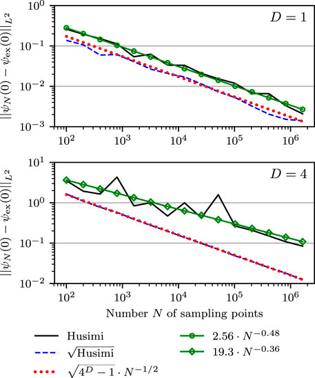
FIGURE 2. Sampling error of the initial wavefunction in one (upper panel) and four (lower panel) dimensions as a function of the number N of Monte Carlo points. The plot displays the error for sampling from the Husimi density (Case H) and its approximated convergence (marked lines) as well as the error for sampling from the square root of the Husimi density (Case sqrt-H) and its analytical error estimation (dotted line).

FIGURE 3

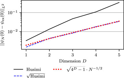
FIGURE 3. Dependence of the sampling error of the initial wavefunction on dimension D for N = 100 ⋅ 2¹³ ≈ 8 ⋅ 10⁵ points sampled from either the Husimi density (Case H) or its square root (Case sqrt-H). The analytical error estimate for the latter sampling is shown by the dotted line.

4.2 Harmonic potential

To analyze the effect of dynamics on the convergence, let us consider a harmonic potential V(x) = x ²/2 in one dimension and explore the dynamics for one full oscillation period. The initial Gaussian wavepacket is still localized in z ₀ = (−1, 0) with width γ = 2. In Figure 4, we compare the exact wavefunction (47) with the numerical realization of the Herman–Kluk propagator which uses the exact solution to q(t), p(t), S(t, z) and R(t, z) stated in Eqs 49, 50, 52, 54. Since the Herman–Kluk propagator is exact for harmonic motion and since we supply exact classical trajectories, the observed numerical error is only due to the Monte Carlo integration. The upper panel of Figure 4 shows the time dependence of the L ²-error

‖ | ψ_{N} (t) 〉 - | ψ_{ex} (t) 〉 ‖_{L^{2}}, (59)

where the semiclassical wavefunctions were generated using N = 2¹⁶ trajectories. Sampling from the square root of the Husimi density (Case sqrt-H) results in approximately twice smaller error than sampling from the Husimi density itself. For (Case sqrt-H), the figure also displays the analytical error estimate derived in (55), which matches the numerical error up to small statistical noise. To remove this statistical noise and to match the analytical estimate (55) more accurately, in the lower panel of Figure 4 we plot the empirical root mean square error (RMSE) [59] S ₁₀₀, where

S_{K} := \frac{1}{K} \sum_{j = 1}^{K} ‖ | ψ_{N}^{(j)} (t) 〉 - | ψ_{ex} (t) 〉 ‖^{2}, (60)

K is an integer number of independent simulations (indexed by j) and each $ψ_{N}^{(j)}$ was itself approximated using N independent samples. One can see that

E [S_{K}] = E [‖ | ψ_{N} (t) 〉 - | ψ_{ex} (t) 〉 ‖^{2}] = \frac{V [| \tilde{ψ} (t) 〉]}{N} . (61)

For K = 1, one obtains the result represented in the upper panel of Figure 4. For K → ∞, due to the strong law of large numbers, S _K converges almost surely to its expectation value and hence to the analytical error estimate.

FIGURE 4

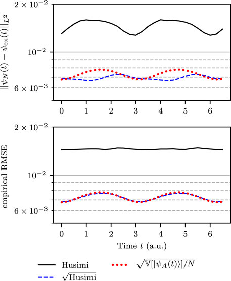
FIGURE 4. Time dependence of the sampling error of the Herman–Kluk wavefunction propagated in a harmonic oscillator. The upper panel is produced by one run with N = 2¹⁶ = 65,536 trajectories, whereas the lower panel is produced by K = 100 independent runs, each with N = 2¹⁶ = 65,536 trajectories, and averaging the square of the error over the K runs. The analytical error estimate for the sampling from the square root of the Husimi density (Case sqrt-H) is shown with the dotted line.

The lower panel of Figure 4 shows the empirical RMSE computed with K = 100 and N = 2¹⁶. For (Case sqrt-H), it coincides almost perfectly with the analytical prediction. We note that the error reaches its maximum whenever the wavefunction passes through the bottom of the potential and its minimum when the wavefunction arrives at the turning points. Even though this analysis makes only sense for finite variance, the figure also displays the empirical RMSE for (Case H), which is nearly constant. Both panels show a qualitatively similar error evolution for (Case H), however, at a magnitude that is considerably larger than the error for (Case sqrt-H).

4.3 Morse potential

To investigate the convergence of the Herman–Kluk wavefunction in anharmonic systems, we consider dynamics generated by a less and more anharmonic Morse potentials. The parameters were taken from [29]. Our initial state is a Gaussian wavepacket with zero initial position and momentum (q ₀, p ₀) = (0, 0), and with a width parameter γ = 0.00456 a.u. $\approx 1000 {cm}^{- 1}$ . The Morse potential

V (x) = V_{eq} + D_{e} {[1 - e^{- a (x - q_{eq})}]}^{2} (62)

is characterized by the dissociation energy D _e, decay parameter a, and the position q _eq and energy V _eq of the minimum. We considered two Morse potentials, both with V _eq = 0.1 and q _eq = 20.95 a.u., but with different values of a and D _e. The latter two parameters, however, were chosen so that the global harmonic potential fitted to the Morse potential at q _eq had the same frequency

ω_{eq} = \sqrt{V^{''} (q_{eq})} = \sqrt{2 D_{e} a^{2}} = 0.0041 a.u. \approx 900 {cm}^{- 1} (63)

for the two Morse potentials. The anharmonicity of the potentials was conveniently controlled with the dimensionless parameter

χ = ℏ \frac{ω_{eq}}{4 D_{e}}, (64)

which is also reflected in the bound energy levels [71]

E_{n} = ℏ ω_{eq} [(n + \frac{1}{2}) - χ {(n + \frac{1}{2})}^{2}] (65)

of a Morse oscillator. Then D _e and a are given by

\begin{aligned} D_{e} & = ℏ \frac{ω_{eq}}{4 χ}, \\ a & = \sqrt{2 \frac{ω_{eq} χ}{ℏ}} . \end{aligned} (66)

We choose two different values

χ = 0.005 and χ = 0.01 (67)

of anharmonicity and compare the Herman–Kluk propagation with a grid-based reference quantum calculation obtained by the Fourier-split method [72], which is second-order accurate with respect to the time step. The position grid was set from x = −200 to 1500 with 4096 equidistant points for χ = 0.005 and from x = −200 to 10,000 with 16,384 equidistant points for χ = 0.01. The larger grid for χ = 0.01 was required to capture oscillations of the wavefunctions in the tail region, which are due to the increased anharmonicity. For the time propagation of the Herman–Kluk wavefunction, we used a second order Størmer-Verlet scheme with step size Δt = 8 a.u. $\approx 0.194$ fs.

Because the Herman–Kluk approximation is not exact in a Morse potential, to separate the statistical convergence error from the semiclassical error of the fully converged Herman–Kluk approximation, in Figure 5 we show the L ²-error

‖ ψ_{N} (t) - ψ_{2 N} (t) ‖ (68)

between the Herman–Kluk wavefunctions calculated with N and 2N trajectories as a function of N. Both wavefunctions were propagated in a Morse potential with anharmonicity χ = 0.005. Each panel includes the error for the fixed time t after approximately one oscillation (196 time steps) and ten oscillations (1960 time steps). In addition, the convergence rates for both sampling schemes were fitted to the same power law (57). We observe that sampling from the square root of the Husimi density (Case sqrt-H), shown in the lower panel, performs better than sampling from the Husimi density (Case H), displayed in the upper panel.

FIGURE 5

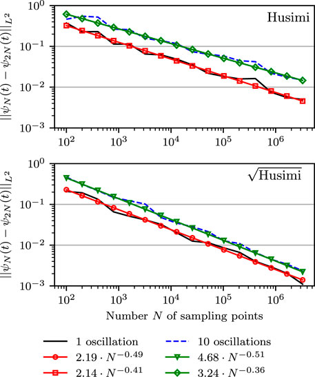
FIGURE 5. Sampling error between the Herman–Kluk wavefunctions obtained with N and 2N Monte Carlo quadrature points as a function of N. The wavefunctions are calculated in a Morse potential with anharmonicity parameter χ = 0.005 after approximately one (solid line) or ten oscillations (dashed line). The upper panel shows both errors and their approximated convergence rates for (Case H). Similarly, (Case sqrt-H) is displayed in the lower panel.

Figure 6 shows the analogous results obtained in a Morse potential with a larger anharmonicity parameter χ = 0.01. Here, we display the wavefunctions after 202 and 2020 time steps, which are approximately the times after the first and tenth oscillations. As expected for anharmonic evolution, the error after ten oscillations is worse than after one oscillation. Increased anharmonicity also increases the error in comparison to Figure 5. Again, the sampling from the square root of the Husimi density (Case sqrt-H) has consistently a lower error than (Case H).

FIGURE 6

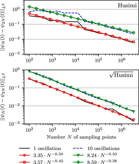
FIGURE 6. Same as Figure 5, except that the anharmonicity parameter of the Morse potential was increased to χ = 0.01.

To complement the abstract convergence study of the L ²-error, in the upper panels of Figures 7 and 8, we compare the more intuitive position probability densities of the “exact” quantum grid-based solution with those of (Case H) and (Case sqrt-H). Both figures were obtained in a Morse potential with anharmonicity parameter χ = 0.01 at a time after ten oscillations. The difference lies in the number of trajectories used. The less converged results in Figure 7 were obtained with only N = 800 trajectories, whereas the fully converged results in Figure 8 employed N = 100 ⋅ 2¹⁴ trajectories. The lower panels of the two figures display the absolute errors of the position density for the two cases, measured with respect to the “exact” grid-based position density. The two panels of Figure 7 confirm again that sampling from the square root of Husimi density (Case sqrt-H) results in faster convergence than sampling from the Husimi density (Case sqrt-H). The upper panel of Figure 8 shows that in the numerically converged regime, the Herman–Kluk propagator approximates the exact solution in this system very well, regardless whether one samples from the Husimi density or its square root. The fact that results are numerically converged is confirmed in the lower panel of Figure 8, where the errors of (Case H) and (Case sqrt-H) are approximately the same, which implies that the common remaining error is the error of the Herman–Kluk approximation and not the phase-space discretization error.

FIGURE 7

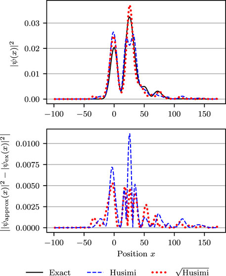
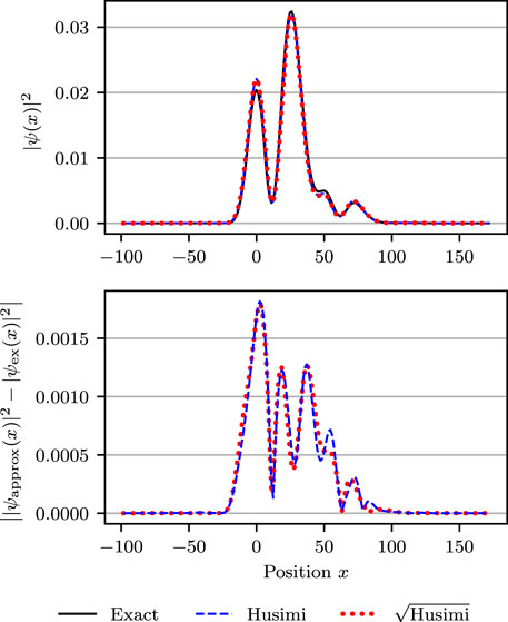
FIGURE 7. Position probability densities (upper panel) and their absolute errors (lower panel) in a Morse potential with χ = 0.01 after 10 oscillations (2020 time steps $\approx 392$ fs). Position probability densities of the Herman–Kluk approximation for (Case H) and (Case sqrt-H) were computed with N = 800 trajectories.

FIGURE 8

FIGURE 8. Same as Figure 7, except that the results were computed with N = 100 ⋅ 2¹⁴ ≈ 1.6 ⋅ 10⁶ trajectories and, therefore, are converged.

Analytical expressions and numerical fits to the convergence rates for all studied systems are summarized in Table 1.

TABLE 1

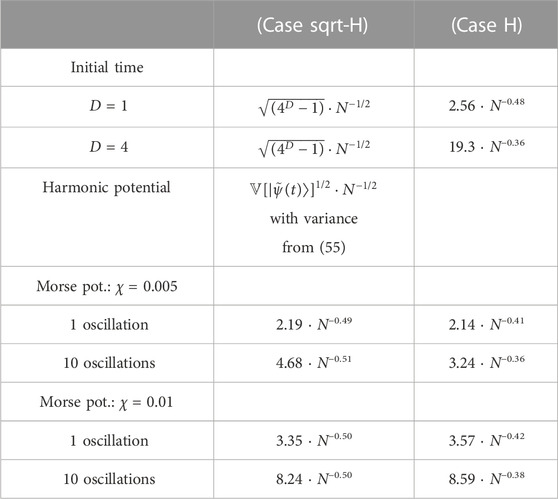
TABLE 1. Summary of convergence rates for (Case sqrt-H) and (Case H) at initial time, in a harmonic oscillator and in two Morse potentials after one and ten oscillations.

Finally, we note that Figure 1 in the Introduction was based, as Figure 8, on the Morse potential with anharmonicity parameter χ = 0.01 and Herman–Kluk calculations used N = 100 ⋅ 2¹⁴ trajectories. For the computation of the position density, we used the more efficient (Case sqrt-H). The spectra in the upper panel were obtained by the Fourier transform of the wavepacket autocorrelation function; the Herman–Kluk autocorrelation function was computed by sampling from the Husimi density (Case H), because it gives the exact result (=1) at t = 0 regardless of the number of trajectories and, therefore, converges faster at short times.

5 Conclusion and outlook

We compared two different sampling strategies for evaluating the semiclassical wavefunction evolved with the Herman–Kluk propagator. For the initial phase-space sampling, we either used the Husimi density (Case H) or its square root (Case sqrt-H). We showed that the square root sampling produces a Monte Carlo integrand with finite second moment, while the Husimi sampling comes with an undesirable infinite second moment. The numerical experiments for the harmonic oscillator and two Morse oscillators with different extents of anharmonicity confirm that the infinite second moment results in a slower convergence of the Monte Carlo estimator. Therefore, we recommend the square root approach (Case sqrt-H) whenever the Herman–Kluk propagator is used directly for approximating the quantum-mechanical wavefunction and the L ²-error of the wavefunction approximation is the relevant accuracy measure. However, we explicitly verified that at initial time the square root density’s second moment, even though it is finite, has an unfavorable, exponential dependence on the dimension, possibly leading to a large number of trajectories required for a reasonably accurate wavefunction.

Although the wavefunction is a central object in quantum mechanics, one is often interested directly in observables, which can be computed as expectation values. It is clearly inefficient to compute expectation values, such as energy or squared norm, with the Herman–Kluk propagator by computing the wave function first. A follow-up paper, in which an analysis similar to that presented here will be applied to the autocorrelation function as well as to the expectation values is in preparation. In particular, the approach to expectation values proposed in [52] will be analysed in detail. Our present analysis and sampling approaches could, in principle, help increase the efficiency of any Gaussian-based method, although it is difficult to predict the possible implications that the coupling between different Gaussians present in Gaussian basis methods [9, 10] might have for the choice of the optimal sampling density.

Data availability statement

The raw data supporting the conclusion of this article will be made available by the authors, without undue reservation.

Author contributions

All authors have contributed to the design and execution of the research and to the writing of the manuscript. FK performed all numerical calculations and prepared all figures.

Acknowledgments

The authors acknowledge financial support from the European Research Council (ERC) under the European Union’s Horizon 2020 Research and Innovation Programme (Grant Agreement No. 683069–MOLEQULE) and from the EPFL.

Conflict of interest

The authors declare that the research was conducted in the absence of any commercial or financial relationships that could be construed as a potential conflict of interest.

Publisher’s note

All claims expressed in this article are solely those of the authors and do not necessarily represent those of their affiliated organizations, or those of the publisher, the editors and the reviewers. Any product that may be evaluated in this article, or claim that may be made by its manufacturer, is not guaranteed or endorsed by the publisher.

Supplementary Material

The Supplementary Material for this article can be found online at: https://www.frontiersin.org/articles/10.3389/fphy.2023.1106324/full#supplementary-material

References

1. Miller WH. Classical S matrix: Numerical application to inelastic collisions. J Chem Phys (1970) 53:3578–87. doi:10.1063/1.1674535

ORIGINAL RESEARCH article

Sampling strategies for the Herman–Kluk propagator of the wavefunction

1 Introduction

2 Discretising the Herman–Kluk propagator

2.1 Herman–Kluk propagator

2.2 Discretisation

2.3 Summary of the numerical algorithm

3 Phase space error analysis

3.1 Moments of the integrand

3.2 Mean squared error

3.3 Other sampling densities

3.4 Harmonic motion

4 Numerical examples

4.1 Initial phase-space error

4.2 Harmonic potential

4.3 Morse potential

5 Conclusion and outlook

Data availability statement

Author contributions

Acknowledgments

Conflict of interest

Publisher’s note

Supplementary Material

References

This article is part of the Research Topic

People also looked at