Time-resolved velocity mapping at high magnetic fields: A preclinical comparison between stack‐of‐stars and cartesian 4D-Flow
 Ali Nahardani1,2*
  Martin Krämer1,3
  Mahyasadat Ebrahimi4,5
  Karl-Heinz Herrmann1 Simon Leistikow6
  Lars Linsen6 Sara Moradi2
  Jürgen R. Reichenbach1
  Verena Hoerr1,2,7*
- 1Medical Physics Group, Institute of Diagnostic and Interventional Radiology, Jena University Hospital, Friedrich Schiller University Jena, Jena, Germany
- 2Heart Center Bonn, Department of Internal Medicine II, University Hospital Bonn, Bonn, Germany
- 3Institute of Diagnostic and Interventional Radiology, Jena University Hospital, Friedrich Schiller University Jena, Jena, Germany
- 4Leibniz-Institute of Photonic Technology, Jena, Germany
- 5Institute of Physical Chemistry and Abbe Center of Photonics, Friedrich Schiller University Jena, Jena, Germany
- 6Department of Mathematics and Computer Science, Institute of Computer Science, Westfälische Wilhelms-Universität Münster, Münster, Germany
- 7Translational Research Imaging Center (TRIC), Clinic of Radiology, University of Münster, Münster, Germany
Purpose: Prospectively-gated Cartesian 4D-flow (referred to as Cartesian-4D-flow) imaging suffers from long TE and intensified flow-related intravoxel-dephasing especially in preclinical ultra-high field MRI. The ultra-short-echo (UTE) 4D-flow technique can resolve the signal loss in higher-order blood flows; however, the long scan time of the high resolution UTE-4D-flow is considered as a disadvantage for preclinical imaging. To compensate for prolonged acquisitions, an accelerated k0-navigated golden-angle center-out stack-of-stars 4D-flow sequence (referred to as SoS-4D-flow) was implemented at 9.4T and the results were compared to conventional Cartesian-4D-flow mapping in-vitro and in-vivo.
Methods: The study was conducted in three steps (A) In-vitro evaluation in a static phantom: to quantify the background velocity bias. (B) In-vitro evaluation in a flowing water phantom: to investigate the effects of polar undersampling (US) on the measured velocities and to compare the spatial velocity profiles between both sequences. (C) In-vivo evaluations: 24 C57BL/6 mice were measured by SoS-4D-flow (n = 14) and Cartesian-4D-flow (n = 10). The peak systolic velocity in the ascending aorta and the background velocity in the anterior chest wall were analyzed for both techniques and were compared to each other.
Results: According to the in-vitro analysis, the background velocity bias was significantly lower in SoS-4D-flow than in Cartesian-4D-flow (p < 0.05). Polar US in SoS-4D-flow influenced neither the measured velocity values nor the spatial velocity profiles in comparison to Cartesian-4D-flow. The in-vivo analysis showed significantly higher diastolic velocities in Cartesian-4D-flow than in SoS-4D-flow (p < 0.05). A systemic background bias was observed in the Cartesian velocity maps which influenced their streamline directions and magnitudes.
Conclusion: The results of our study showed that at 9.4T SoS-4D-flow provided higher accuracy in slow flow imaging than Cartesian-4D-flow, while the same measurement time could be achieved.
1 Introduction
4D phase contrast magnetic resonance imaging, commonly known as 4D-flow, is a technique in cardiovascular MRI for quantifying blood velocity in the 3D space along time [1]. For this purpose, multiple sets of bipolar velocity encoding gradients are applied 3D to sensitize the MRI signal to fast moving spins [2]. Since the quantification of the velocity requires a baseline measurement to subtract the phase of the signal of the dynamic spins, a variety of velocity encoding methods have been emerged which differ in their number of gradients and in accuracy. However, the imbalanced and balanced 4-point methods have become popular since they require the least number of gradients while exhibiting low bias [3–5].
The type of velocity encoding scheme is not the only factor influencing the accuracy of the measured velocity maps. It has been shown that the k-space trajectory has also an impact on accuracy, especially at ultra-high-fields (UHF) [3, 6, 7].
Basically, 4D-flow imaging using Cartesian trajectory has been extensively investigated not only at low fields [8], but also at UHFs [9, 10]. It has been widely used in preclinical MRI (i.e., at UHFs) and benefits from a simple reconstruction pipeline which is compatible with the existing acceleration techniques [8, 11]. However, acceleration by means of the partial coverage of the k-space can influence the accuracy of the velocity maps that may not be recoverable by advanced reconstruction algorithms (such as compressed sensing) [12]. Since the Cartesian trajectory requires multiple imaging gradients overlapping on each other, the gradient duty cycle of this technique is usually high. To tackle this problem, the gradients durations must be increased, influencing the minimum echo time (TE), which is typically >2–3 ms (Figure 1). Such a long TE can result in low signal-to-noise ratio (SNR), low velocity-to-noise ratio (VNR), and in an intensified signal loss in the disturbed flow at UHFs [6] which cannot even be resolved by shortening TE using asymmetric echo acquisition [3]. Moreover, the imaging encoding gradients in the 3D-Cartesian trajectory (i.e., the two phase encoding gradients, bipolar readout gradient, etc.) are experienced as extra velocity sensitizing gradients and result in a higher actual velocity encoding value (VENC) than the nominal value [13].
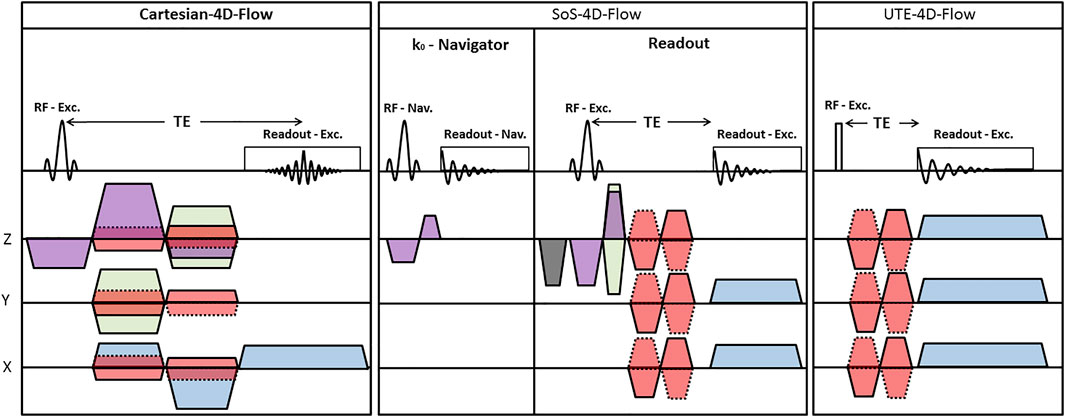
FIGURE 1. Schematic representation of (left) the prospectively-triggered Cartesian-4D-flow; (middle) k0-navigated golden-angle center-out SoS-4D-flow; and (right) UTE-4D-flow pulse sequences. (Purple: Slice/Slab-selection gradient; Gray: Slice/Slab spoiler gradient; Green: Phase encoding gradient; Red: velocity encoding gradient; Blue: Readout gradient).
To increase the accuracy of velocity mapping at UHFs, the ultra-short-echo (UTE) 4D-flow sequence has been introduced [3]. Since a very shortly durated rectangular radiofrequency (RF) pulse is applied in UTE-4D-flow and it requires no slice and phase encoding gradients, the corresponding TEs are sufficiently short (≈500 µs, Figure 1) to preserve the signal in the regions with higher-order blood flows [3]. Additionally, the center of the k-space is densely sampled in this technique; leading to a high SNR and VNR [3, 14–17]. UTE-4D-flow is also compatible with advanced acceleration techniques [7] but at the cost of higher complexity in reconstruction compared to the Cartesian data. Although the temporal resolution of UTE-4D-flow is superior to any Cartesian techniques (due to its typical shorter repetition time—TR), its total scan time is 9.8 times (i.e., π2) longer to satisfy the Nyquist–Shannon sampling theorem for similar scan parameters, which is based on the fact that the coverage of radial spokes should create equidistant solid angles by π projections along the kz direction and 2π projections in the kxy plane.
Moreover, the choice of the gating strategy can influence the total scan time and the quality of velocity maps; especially in small animals due to their rapid heart and respiratory rates. For preclinical imaging at UHFs, the gating efficiency of the prospective triggering method has been reported to be about 50% because of the poor quality of electrocardiograms (ECG), the induction of noise by switching gradients, and long respiratoty delays [3, 18]; nonetheless, it was improved to around 60% in self-gating [3].
When aiming for 4D-flow imaging with reasonable spatial resolution, using the UTE-4D-flow technique is not justifiable due to its long scan time regardless of its very good image quality. To reduce the total scan time and still benefit from the advantages of UTE (i.e., short TE, high SNR, and high VNR), we implemented an efficient k0-navigated golden-angle center-out stack-of-stars 4D phase-contrast imaging sequence (referred to as SoS-4D-flow in the context of this manuscript) as a hybrid combination of the half-spoke radial and Cartesian sampling techniques and investigated the results in-vitro and in-vivo in comparison to those obtained by the conventional prospectively-triggered Cartesian-4D-flow method (called Cartesian-4D-flow in the following).
2 Methods
2.1 Imaging experiments
2.1.1 In-vitro
Two types of phantoms were used for the evaluations (A) Static water phantom, i.e., a simple 50 ml conical tube filled with agar and a small Lego brick inside; (B) Flowing water phantom, i.e. a large cylinder with the inner diameter of 26.1 mm containing water and enclosing four smaller tubes with the inner diameter of 3 mm, which are connected to a water pump with adjustable flow rates of 0, 200, 400, 600, 800 ml/s to produce laminar flows with different speeds. Imaging was carried out on a 9.4T BioSpec USR 94/20 MRI system with ParaVision 6.0.1 (Bruker BioSpin MRI GmbH, Ettlingen, Germany) using a vendor-supplied 72-mm-diameter transmitter and receiver volume coil with the sequences and parameters listed in Table 1.
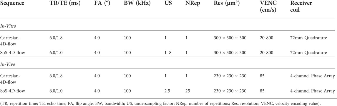
TABLE 1. Summary of the applied sequences and their corresponding parameters.
2.1.2 In-vivo
24 male C57BL/6 mice were included in the study and divided into two experimental groups (A) 10 animals were scanned with the prospectively-triggered Cartesian-4D-flow sequence; (B) 14 animals were investigated with the k0-navigated golden-angle SoS-4D-flow technique. It is important to note that SoS-4D-flow was performed by 25 repetitions for retrospective reconstruction and 2.5 undersampling factor (US). A summary of the sequences and parameters is provided in Table 1. All acquisitions were performed with the same hardware settings as in the in-vitro step, except for the coil; a dedicated cardiac 4-channel phased-array was used as receiver instead of the 72 mm Quadrature coil. The study was performed in accordance with the National Institute of Health Guidelines for the Care and Use of Laboratory Animals (eighth edition) and the European Community Council Directive for the Care and Use of Laboratory Animals of 22 September 2010 (2010/63/EU). The study protocol was approved by the competent State Office for Food Safety and Consumer Protection (TLLV, Bad Langensalza, Germany; local registration number: 22-2684-04-UKJ-19-002).
2.2 Pulse sequences
2.2.1 SoS-4D-flow
The k0-navigated golden-angle center-out stack-of-stars 4D phase-contrast velocity mapping was implemented in five steps (A) A vendor-supplied 2D-UTE sequence with ramp-sampling was modified by integrating a 3D phase-encoding gradient along the slice/slab-selection direction to turn it into a 3D-SoS. To shorten TE, the phase encoding gradient was overlapped with the slice/slab-selection rephasing gradient. No phase rewinder gradient was added to reduce TR. (B) The readout spoiler gradient was removed from the sequence; instead, a short and strong slice/slab spoiler gradient was applied next to the slice/slab-selection gradient before the next excitation to compensate for any interference artifacts that could arise in its absence. (C) After the development of a stable version of 3D-SoS with a continuous rotation angle, the golden angle acquisition (with the rotation angle of π(3-√5) = 137.507 between spokes) was integrated in the sequence, which guaranteed good k-space coverage even at high US factors. (D) To retrospectively sort the radial spokes with respect to the physiological motion, an external k0-navigator module was implemented just before the main acquisition block of the sequence. In k0-navigator, a slice-selective short-duration RF-pulse (0.1024 ms) was applied in an arbitrary (user-specified) orientation. The corresponding FID signal was collected in the absence of gradients, which was primarily modulated by the cardiac and/or diaphragmatic motion. (E) The balanced 4-point velocity encoding scheme was integrated in the sequence just after the 3D phase-encoding gradient to sensitize the center-out radial spokes to higher-order motion. The minimum duration of the flow-encoding gradient was calibrated to 0.6 ms as gradient imperfections arose at shorter intervals. After all modifications, a minimum TE ≈ 1 ms could be achieved. A schematic representation of the sequence is illustrated in Figure 1.
2.2.2 Cartesian-4D-flow
A commercially available prospectively-triggered Cartesian-4D-flow sequence (FlowMap, ParaVision 6.0.1, Bruker BioSpin MRI GmbH, Ettlingen, Germany) was used as a reference. The sequence was composed of a balanced 3D gradient-echo and a balanced 4-point velocity encoding scheme. A respiratory bulb and a 3-lead ECG were used to capture the respiratory and cardiac motion and to prospectively synchronize the acquisition with physiological motion. The R-wave of the ECG during the expiratory period was set as the external trigger pulse. A schematic representation of the sequence is illustrated in Figure 1.
2.3 Image reconstruction
2.3.1 In-vitro data
2.3.1.1 SoS-4D-flow
The imaging trajectory was measured by [19] before each acquisition. The corresponding k-space sampling densities were estimated using the trajectory information. The polar signals were gridded by an iterative sampling density compensation algorithm with optimized kernel using an in-house developed MATLAB framework. Finally, a 3D inverse fast Fourier operator (3D-iFFT) was applied on the gridded data to reconstruct the complex images. By the use of the complex images and the following equations, the individual velocity maps were calculated:
Where
2.3.1.2 Cartesian-4D-flow
The in-vitro Cartesian-4D-flow data were reconstructed by the application of 3D-iFFT. The corresponding velocity maps were calculated using Eq 1–3.
2.3.2 In-vivo data
2.3.2.1 k0-navigated SoS-4D-flow
For the in-vivo application of SoS-4D-flow, an external k0-navigator was used. At first, different k0 signal components (i.e., magnitude, phase, imaginary, and real) were visually inspected to identify the optimal domain that best represented the cardiac and respiratory motion. Second, the navigator FID was amplified and summarized by taking the L2-norm of different channels. Third, FID was denoised by the Savitzky-Golay filter, and then the biorthogonal wavelet algorithm was applied to resolve the remaining signal redundancies. Fourth, the inspiration cycles were identified from FID, and the corresponding radial spokes were discarded. Fifth, by considering the peaks of FID as the onsets of the cardiac cycles, the radial signals were sorted according to the heart motion (Figure 2). Since many radial spokes were discarded in the process of retrospective reconstruction, a high degree of sparsity was achieved in the finally-sorted raw-data. Nonetheless, this problem could be resolved by averaging the sparse raw-data over all the acquired 25 repetitions (see the methods section). Eventually, the total variation compressed sensing (CSTV) reconstruction algorithm was applied along the space, time, and velocity domains using the Berkeley Advanced Reconstruction Toolbox (BART) [20] and the corresponding velocity maps were calculated by Eqs 1–3. To adjust for the coil sensitivities, the eigenvalue-based iterative self-consistent parallel imaging reconstruction algorithm (ESPIRiT) was applied [21].
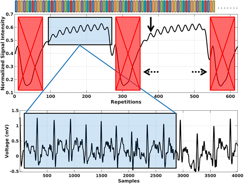
FIGURE 2. Representative image showing the cardiac and respiratory motion modulations in a filtered k0-navigator signal. During the retrospective sorting of the main SoS-4D-flow radial spokes, the inspiration cycles and their corresponding radial spokes were discarded (dashed arrows). The peaks of the cardiac modulations were considered as the onset of the heart cycles and the radial spokes were sorted accordingly (solid arrow). The color bars on top represent different radial spokes.
2.3.2.2 Cartesian-4D-flow
Since the sequence was prospectively-gated, it was not necessary to sort out the raw-data. The applied reconstruction pipeline was the same as for the SoS-4D-flow in-vivo experiments; i.e. all data were reconstructed using CSTV plus ESPIRiT, and the corresponding velocity maps were calculated by Eqs 1–3
2.4 Velocity analysis
2.4.1 In-vitro data
2.4.1.1 Segmentation
An in-house developed semi-automatic segmentation algorithm (using the simultaneous information of the complex images and velocity maps) was applied to label the stationary and dynamic regions within the in-vitro data. All labels were validated visually to ensure for the accuracy of segmentation. In the phantom data, the first and the last 20% of slices along the Z direction were discarded to mitigate the bias of RF imperfections (i.e., the middle 60% of 3D-stacks were extracted and entered statistics).
2.4.1.2 Static phantom
The main purpose of using the static phantom was to evaluate and quantify the background velocity bias. After segmentation, the L2-norms of the velocity maps (i.e., velocity magnitudes) were calculated in both sequences (i.e., SoS-4D-flow and Cartesian-4D-flow), and the mean and maximum background velocity changes were compared statistically. A regression analysis between the maximum velocity and different VENC values was performed in both techniques.
2.4.1.3 Flowing water phantom
The principle goal of using the flowing water phantom was to investigate the accuracy of SoS-4D-flow in comparison to the Cartesian-4D-flow technique, as well as to evaluate the reproducibility of the findings in the static phantom. For this purpose, first, the velocity maps were segmented for the stationary and dynamic regions semi-automatically. Second, the L2-norms of the velocity maps were calculated for both the SoS-4D-flow and Cartesian-4D-flow techniques. Third, to confirm the findings of the static phantom data, the background velocity bias was reevaluated at the stationary portion of the flowing water phantom. Fourth, to compare the VNR efficiencies at different pump speeds, the individual VNRs for both sequences were calculated at the flow rates of 200, 400, 600, and 800 ml/s and were eventually summed-up. The final sum value was used for VNR comparisons. Fifth, to investigate the similarity of the SoS-4D-flow results with the Cartesian-4D-flow velocities, the velocity magnitudes of each technique were regressed to different pump speeds and the regression coefficient were compared. Sixth, to study the k-space trajectory effects on the spatial velocity profiles, the velocities across a representative tube (in which dynamic spins existed) were plotted with respect to their location and the spatial integrals were calculated and compared in both techniques. Last but not least, the effects of polar undersampling on the accuracy of SoS-4D-flow results were investigated by averaging and comparing their velocity values to the fully-sampled Cartesian-4D-flow results.
2.4.2 In-vivo data
For methodological comparison, the velocity maps of SoS-4D-flow and Cartesian-4D-flow were angulated perpendicular to the longitudinal axis of the ascending aorta (AA) and the through-plane velocity components were selected. Region-of-interests (ROI) were drawn manually at the distal AA and the peak systolic velocities (Vmax) were calculated and used for the statistical comparison. In addition, the velocity-time profiles were divided into the diastolic and systolic portions and were integrated over time for comparing the techniques. Finally, the background velocity was measured in the anterior chest wall (ACW) using ROI analysis at the same slice location.
3 Results
3.1 Static phantom
The concept of SoS-4D-flow was implemented on a small animal MRI scanner at 9.4T and the results were compared to those obtained by Cartesian-4D-flow. The qualitative evaluation of the velocity maps in both techniques showed a persistent 3D background velocity bias, with the slope of changes being less in SoS-4D-flow (Figure 3). The analysis of 4D flow data at different VENCs showed significantly lower (62.3% less) background velocity bias in SoS-4D-flow than in Cartesian-4D-flow with the mean values of 7.63 ± 3.47 cm/s vs. 20.28 ± 0.66 cm/s respectively (p < 0.05). The maximum background bias in SoS-4D-flow was on average 19.507 ± 4.23 cm/s and significantly less than the maximum bias in the Cartesian-4D-flow results showing an average value of 42.647 ± 7.105 cm/s (p < 0.05). In both sequences, the maximum background velocity varied with different VENC values. Accordingly, the maximum velocity and the value of VENC showed a significant strong correlation in the Cartesian-4D-flow velocity maps (r = 0.992, p < 0.05), while no significant correlation was observed in the SoS-4D-flow data (r = 0.443, p > 0.05).
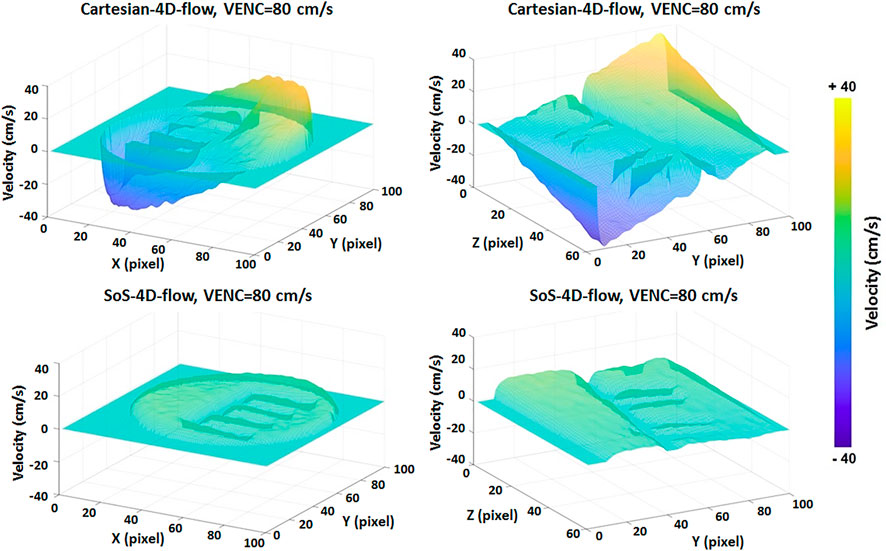
FIGURE 3. Representative image of the static phantom in which the velocity values are supposed to be ideally equal to 0 cm/s showing higher background velocity bias in Cartesian-4D-flow than in SoS-4D-flow. Each unit in pixel along the X,Y, and Z axes represents 300 µm.
3.2 Flowing water phantom
In the flow phantom, consisting of four straight tubes, our analysis showed a background velocity bias comparable to the findings in the static phantom; i.e., the averaged velocity bias in SoS-4D-flow was significantly less (56.7%) than the value inspected in Cartesian-4D-flow (10.75 ± 0.05 vs. 24.87 ± 0.12 cm/s, respectively, p < 0.05). The SoS-4D-flow acquisition with US = 3.15 provided the same scan time as the fully-sampled Cartesian-4D-flow but resulted in an acceptable background velocity bias equal to 9.90 ± 0.11 cm/s. The sum of VNRs (over the flow rates of 200, 400, 600 and 800 ml/s) in Cartesian-4D-flow was considerably less than the sum of VNRs in SoS-4D-flow with the values of 9.911 vs. 21.57 respectively. The sum of VNRs in the SoS-4D-flow acquisition with US = 3.15 was 23.25.
In addition, a significantly strong correlation was observed between the L2-norm of velocity values in the fully-sampled SoS-4D-flow and the Cartesian-4D-flow data over the pump speeds of 200–800 ml/s (r = 0.994, p < 0.05). Furthermore, a strong association was observed between the velocity values measured by the undersampled SoS-4D-flow with US = 3.15 and the Cartesian-4D-flow technique (r = 0.994, p < 0.05). Nevertheless, the agreement between the SoS-4D-flow (with and without US) and the Cartesian-4D-flow technique was reduced at slow velocities (Figure 4E).
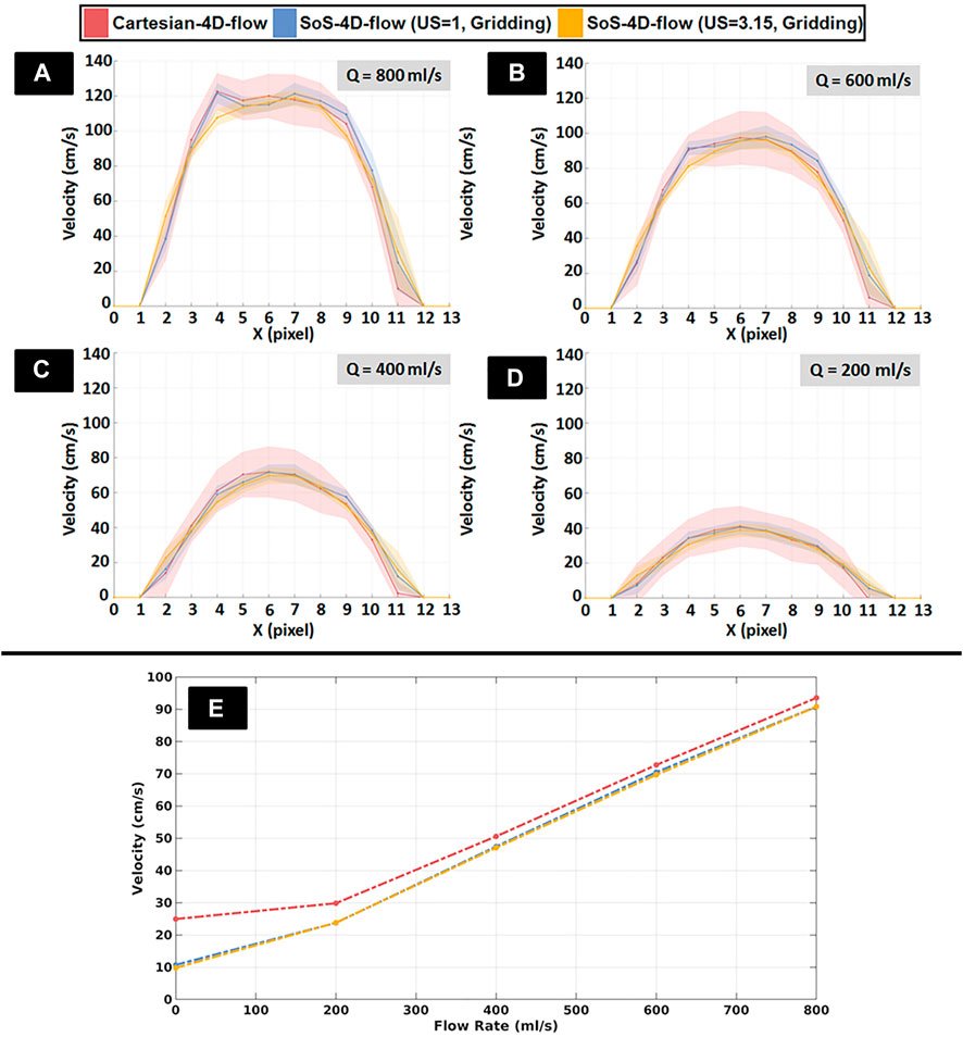
FIGURE 4. (A–D) Representative spatial velocity profiles perpendicular to the long axis of a representative tube (solid lines: mean velocity, shades: standard deviation) obtained from fully sampled SoS-4D-flow, undersampled SoS-4D-flow with an undersampling (US) factor of π, and Cartesian-4D-flow data at different pump speeds (Q) ranging from 200 to 800 ml/s. Each unit in pixel along the X axis represents 300µm. (E) Representative plot showing the velocity values obtained by the fully-sampled SoS-4D-flow, undersampled SoS-4D-flow, and the fully-sampled Cartesian-4D-flow technique at different flow rates (i.e., pump speeds).
With respect to the effect of polar undersampling on the accuracy of velocity maps, neither an underestimation nor overestimation was observed in the SoS-4D-flow velocity values at different US factors in the range of 1.0–8.0, showing an averaged velocity value of 92.27 ± 1.08 cm/s in comparison to the velocity value of 93.52 cm/s measured by the fully-sampled Cartesian-4D-flow technique (Table 2).
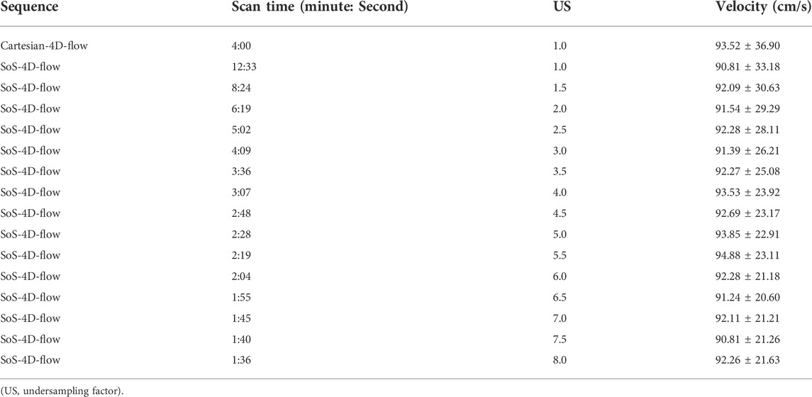
TABLE 2. In-vitro comparison of the velocity values of multiple SoS-4D-flow measurements with different undersampling factors to the reference value obtained by the fully-sampled Cartesian-4D-flow technique.
The shape of the spatial velocity profiles in the SoS-4D-flow velocity maps (with US = 1 and US = 3.15) was preserved in comparison to the Cartesian-4D-flow technique; i.e., the spatial integral of the velocities measured by the fully-sampled SoS-4D-flow, undersampled SoS-4D-flow (with US = 3.15), and the fully-sampled Cartesian-4D-flow technique were 931.20, 908.78 and 911.91 cm/s respectively at the pump speed of 800 ml/s, while they changed to 266.61, 262.53 and 266.23 cm/s at the pump speed of 200 ml/s respectively (Figure 4A–D).
In regard to the velocity visualization, the background velocity field imposed a systematic vector alteration in the Cartesian-4D-flow results, influencing both the magnitudes and the directions of the corresponding velocity vector fields, which was more prominent at slow pump speeds (Figure 5).
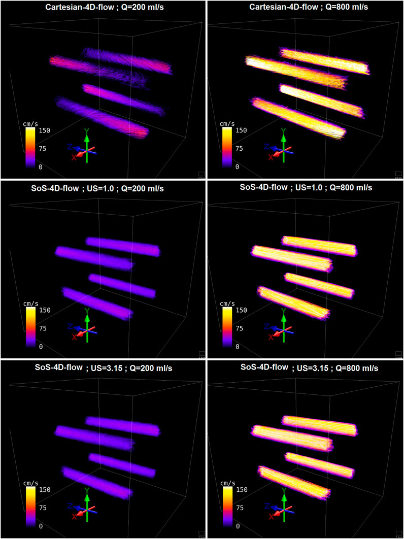
FIGURE 5. Representative streamline visualization of the in-vitro flowing water phantom reconstructed from fully-sampled SoS-4D-flow, undersampled SoS-4D-flow (by a factor of π), and Cartesian-4D-flow data at high and low pump speeds (Q value).
3.3 In-Vivo analysis
For in-vivo blood flow analysis, the SoS-4D-flow sequence was extended by k0-navigation and CSTV reconstruction. No significant differences were observed between the Vmax values of the SoS-4D-flow and Cartesian-4D-flow results in AA (91.83 ± 13.18 vs. 92.61 ± 9.57 cm/s respectively, p > 0.05). However, the sum of the diastolic velocities differed significantly between both sequences (SoS-4D-flow: 24.23 ± 5.41 vs. Cartesian-4D-flow: 82.88 ± 30.38 cm/s, p < 0.05). Nevertheless, the sum of the systolic velocities showed no significant difference between the SoS-4D-flow and Cartesian-4D-flow result (449.96 ± 88.13 vs. 520.83 ± 73.29 cm/s respectively, p > 0.05) (Figure 6, E). The velocity-time curves of both the techniques showed a significant linear correlation (r = 0.995, p < 0.05) to each other. The averaged background velocity over ACW was significantly less in the SoS-4D-flow velocity maps compared to the Cartesian-4D-flow data with the average values of 3.29 ± 0.95 vs. 14.29 ± 5.49 cm/s respectively (p < 0.05). Qualitatively, the streamline directions of Cartesian-4D-flow were influenced by the concomitant field in-vivo showing distracted flow directions in aorta, while the streamlines of the SoS-4D-flow techniques were preserved and represented the expected orientations (Figure 6A–D). The average scan time of the Cartesian-4D-flow and the SoS-4D-flow technique were 70.32 ± 4.33 and 68.74 ± 8.73 minutes orderly.
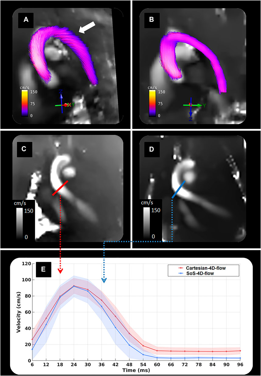
FIGURE 6. Representative figure showing (A) Streamline visualization of an in-vivo data obtained by Cartesia-4D-flow; (B) Streamline visualization of an in-vivo data obtained by SoS-4D-flow; (C) A velocity map of an in-vivo data acquired by Cartesian-4D-flow; (D) A velocity map of an in-vivo data measured by SoS-4D-flow; (E) Velocity-time curves at the cross-section of the distal ascending aorta obtained by the k0-navigated SoS-4D-flow and the prospectively-triggered Cartesian-4D-flow technique. Please note that the strong background velocity in the Cartesian-4D-flow data has influenced the streamline orientation in aorta (solid white arrow), while the streamline quality is well-preserved in the SoS-4D-flow results.
4 Discussion
Historically, the concept of 4D-flow imaging emerged in the late 1990s [22, 23] and has been continuously refined through improvements in velocity encoding methods [4, 24–27], spatial encoding trajectories [7, 28–31] and reconstruction pipelines [32, 33]. It has already been reported that TE shortening could reduce intravoxel-dephasing of higher-order motions, such as found in turbulent flows [34, 35]. Accordingly, O'Brien et al. introduced a UTE-2D-flow sequence with TE ≈ 0.65 ms to recover the signal from high-velocity turbulent jets after the presence of stenosis [36].
With the initial introduction of the stack-of-stars phase contrast angiography at 3.0T by Kecskemeti et al., the minimum achievable TE was 3.7 ms due to full spoke readout from -k to + k [37], which was considered an appropriate TE for angiographic purposes but not for velocity mapping. Kadbi et al. adopted the concept of center-out acquisition from [36] and combined it with [37] to design a SoS-4D-flow with TE ≈ 1 ms at 1.5T [6]. However, their study was mainly investigated in-vitro and did not include any comprehensive evaluations in-vivo. Up to our knowledge, the application of the center-out SoS-4D-flow sequence has not been investigated in UHFs, neither in human nor small animal imaging.
Since the prospectively-triggered Cartesian-4D-flow velocity mapping requires long gradient duration as well as a bipolar readout gradient to cover–k to + k line by line, its typical TEs are long enough to be considered as an disadvantage in the regions of higher blood flow at 9.4T because of signal cancellation. For this purpose, we implemented a golden-angle center-out SoS-4D-flow sequence at 9.4T with reduced TE ≈ 1 ms and evaluated it in-vitro and in-vivo.
Our in-vitro investigations in the static phantom showed a notable background velocity deviation in the Cartesian-4D-flow velocity maps, which was dependent on the location of the voxel and was persistent in different VENC values, tending to increase with higher velocity sensitizing gradient amplitudes. Since the reduction of TE in UHF systems is crucial to compensate for the intensified intravoxel-dephasing, it is a common practice to overlap all gradient events (i.e., slice, phase, readout, etc.) in the design of Cartesian sequences. The design of the standard Cartesian-4D-flow sequence at 9.4 T is not an exception from this convention. Since all gradient events overlap along the X, Y, and Z directions in the Cartesian-4D-flow technique, the net gradient amplitude along each physical coordinate is very strong. This led to the formation of a strong concomitant filed (Maxwell field) and consequently to a huge phase drift throughout the object—which is the main source of the observed significant background velocity bias in the Cartesian-4D-flow data. As reported by Bernstein et al. [38] and Norris et al. [39], the gradient polarity does not have any influence on the phase drift and thus the reconstruction of the velocity maps using Eqs 1–3 could not unwrap and correct the signal. Based on [38], the velocity drift has to be dependent on both the voxel location and the net gradient amplitude along the physical axes, which was in accordance with our observations; i.e. we observed that the strongest velocity drift existed at the diagonal axis from the gradient isocenter at the end points of FOVs. The background velocity bias due to the Maxwell field was significantly (p < 0.05) reduced in SoS-4D-flow since it had fewer overlapping gradients.
Similar to the static phantom, a big velocity drift was observed in the results of the flowing water phantom. When a comparison was drawn between the velocity maps acquired by SoS-4D-flow and Cartesian-4D-flow at different pump speeds, we observed that the Maxwell field changed the streamline directions in Cartesian-4D-flow at slow flow rates (i.e., slow velocities). However no obvious changes were detected in the streamlines reconstructed from the SoS-4D-flow data at the same pump speed (Figure 5). Therefore, it is predictable that the presence of strong concomitant fields in the Cartesian-4D-flow sequence at short TE can limit its application at UHFs for imaging at high resolutions and low VENC values since both conditions increase the net gradient amplitudes. Additionally, we observed that the effect of the concomitant field on the total velocity vector field of the Cartesian-4D-flow technique was still persistent but less prominent at fast flow rates (i.e., at fast velocities) (Figure 5).
Our in-vivo findings were in accordance with the in-vitro results, with respect to a higher background velocity observed in Cartesian-4D-flow compared to SoS-4D-flow. By having a closer look at the corresponding velocity-time curves (Figure 6E), the difference in the hemodynamic profiles was more prominent during the diastolic period than in the systole, suggesting that for the evaluation of slow velocities (such as the diastolic velocity profiles) the application of SoS-4D-flow can be superior to Cartesian-4D-flow at UHFs. Since the reconstruction algorithm of both techniques was the same, the difference could not originate from the reconstruction pipeline but rather from the sequence itself. Furthermore, the integration of the SoS-4D-flow technique with the k0-navigator pulse and retrospective reconstruction could increase the quality of its velocity maps in two additional ways; (A) the poor quality ECG was replaced by a strong navigator signal, which decreased the possible errors originating from the triggering method; (B) for retrospective reconstructions, we scanned the whole k-space with 25 repetition, then sorted the signals and averaged each sorted k-space over all the 25 repetitions. This part of the pipeline could reduce the thermal noise in the source complex images and could increase the VNR in the final velocity maps.
According to [40, 41], anesthesia of small animals using Isoflurane can influence the cardiac physiology and the corresponding hemodynamics; hence, shorter scan times are always preferable for cardiac magnetic resonance. In this regard and in comparison to the other sophisticated sequences such as UTE-4D-flow (which covers the whole k-space center-out radially), we believe that the application of SoS-4D-flow could be more advantageous despite of its less expected VNR. Since the size of the imaging matrix is a determinant factor on the number of the required projections in UTE-4D-flow; high resolution imaging with large field-of-views (FOV) could limit the application of UTE-4D-flow due to time constraints. For instance, in a previous investigation on the UTE-4D-flow technique, the total scan time at the resolution of the current study (i.e., 230 μm) was ≈2 h with TR = 3.1 ms [3], while the total scan time of SoS-4D-flow was ≈68 minutes with TR = 6 ms (i.e., the hybrid characteristics of SoS-4D-flow could save time since the π factor of additional projections along the slice/slab directions is not further required). It is not yet known whether the simultaneous applications of three readout gradients in the UTE-4D-flow technique have any significant impact on the formation of Maxwell fields or not, especially at high resolutions. Thus, further investigations are recommended to compare the Maxwell fields in the SoS-4D-flow sequence with those in the UTE-4D-flow technique. For an accurate comparison, according to the methodology presented in [3], we suggest to use a spatially nonselective RF pulse in the absence of any slice/slab selection gradients to minimize TE and the net gradient amplitude in SoS-4D-flow. Since UTE-4D-flow is based on the Kooshball trajectory, it would be invaluable to additionally investigate the effects of the polar undersampling on the accuracy of the resultant velocity maps in comparison to the fully accelerated SoS-4D-flow technique. However, this investigation was not in the scope of this research and will require further studies.
Since we used no Cartesian acceleration along the kz-direction in SoS-4D-flow (i.e., we used only polar undersampling in the kxy plane), we decided to apply no Cartesian undersampling in the reference 4D-flow measurements (i.e., Cartesian-4D-flow). This approached could eliminate the corresponding confounding factors in the final statistical analysis. Accordingly, it is not clear how the results of those two methods would deviate if a full Cartesian acceleration was applied. Hence, we suggest a deeper investigation to address this issue.
Physically, there are only two remedies to reduce the concomitant fields in Cartesian-4D-flow (A) to separate the imaging and velocity encoding gradients from each other, which increases TE and signal loss at UHFs, especially in the regions with the higher order blood flow; (B) to use coarser spatial resolutions or higher VENC values to use a weaker gradient strength. Despite of the applicability of those approaches in big in-vivo objects (such as humans), they limit the application of the Cartesian-4D-flow in small animal imaging since high resolutions and short TE are always required. Analytically, the effect of concomitant fields can also be corrected by solving a fitting problem; nevertheless, the sole application of the model-based correction methods is subject to inaccuracies [42]. Accordingly, the model-based corrections can add bias into the regions where real velocities exist. Thus, the optimum correction of the Maxwell field additionally necessitates modifying the gradient events [38]. Based on this, SoS-4D-flow has little gradient overlaps and results in a negligible concomitant field. In addition, it benefits from a short TE at UHFs, which preserves the accuracy of estimated velocities [6]. To this end, we come into the conclusion that the SoS-4D-flow technique is not only suitable to accurately quantify fast velocities requiring short TEs, but also is a precise method for the estimation of a wide range of velocities including slow flows.
Data availability statement
The raw data supporting the conclusion of this article will be made available by the authors, without undue reservation.
Ethics statement
The animal study was reviewed and approved by the State Office for Food Safety and Consumer Protection (TLLV, Bad Langensalza, Germany).
Author contributions
AN: Conceptualization, sequence design, data acquisition, image reconstruction, image and statistical analysis, validation, visualization, original draft preparation, review and editing. MK: Conceptualization, sequence design, image reconstruction, image analysis, validation, review and editing. ME: data acquisition, validation, review and editing. K-HH: sequence design, validation, review and editing. SL: Image analysis, review and editing. LL: Image analysis, review and editing. SM: Image and statistical analysis, validation, review and editing. JR: Conceptualization, validation, review and editing, project administration. VH: Conceptualization, sequence design, data acquisition, image and statistical analysis, validation, review and editing, project administration. All authors have read and agreed to the published version of the manuscript.
Funding
This study was supported by the German Research Foundation (Deutsche Forschungsgemeinschaft/DFG, Project-ID: 468824876 granted to VH and LL).
Acknowledgments
Parts of this work will be used in the doctoral thesis of AN. We would like to thank Van Nhat Minh Vo for his support.
Conflict of interest
The authors declare that the research was conducted in the absence of any commercial or financial relationships that could be construed as a potential conflict of interest.
Publisher’s note
All claims expressed in this article are solely those of the authors and do not necessarily represent those of their affiliated organizations, or those of the publisher, the editors and the reviewers. Any product that may be evaluated in this article, or claim that may be made by its manufacturer, is not guaranteed or endorsed by the publisher.
References
1. Dyverfeldt P, Bissell M, Barker AJ, Bolger AF, Carlhäll C-J, Ebbers T, et al. 4D flow cardiovascular magnetic resonance consensus statement. J Cardiovasc Magn Reson (2015) 17(1):72. doi:10.1186/s12968-015-0174-5
2. Nayak KS, Nielsen J-F, Bernstein MA, Markl M, Gatehouse P D, Botnar R M, et al. Cardiovascular magnetic resonance phase contrast imaging. J Cardiovasc Magn Reson (2015) 17(1):71. doi:10.1186/s12968-015-0172-7
3. Krämer M, Motaal AG, Herrmann KH, Löffler B, Reichenbach JR, Strijkers GJ, et al. Cardiac 4D phase-contrast CMR at 9.4 T using self-gated ultra-short echo time (UTE) imaging. J Cardiovasc Magn Reson (2017) 19(1):39. doi:10.1186/s12968-017-0351-9
4. Pelc NJ, Bernstein MA, Shimakawa A, Glover GH. Encoding strategies for three-direction phase-contrast MR imaging of flow. J Magn Reson Imaging (1991) 1(4):405–13. doi:10.1002/jmri.1880010404
5. Dyverfeldt P, Hope MD, Tseng EE, Saloner D. Magnetic resonance measurement of turbulent kinetic energy for the estimation of irreversible pressure loss in aortic stenosis. JACC: Cardiovasc Imaging (2013) 6(1):64–71. doi:10.1016/j.jcmg.2012.07.017
6. Kadbi M, Negahdar MJ, Cha J, Traughber M, Martin P, Stoddard MF, et al. 4D UTE flow: A phase-contrast MRI technique for assessment and visualization of stenotic flows. Magn Reson Med (2015) 73(3):939–50. doi:10.1002/mrm.25188
7. Braig M, Menza M, Leupold J, LeVan P, Feng L, Ko C-W, et al. Analysis of accelerated 4D flow MRI in the murine aorta by radial acquisition and compressed sensing reconstruction. NMR Biomed (2020) 33(11):e4394. doi:10.1002/nbm.4394
8. Bock J, Töger J, Bidhult S, Markenroth Bloch K, Arvidsson P, Kanski M, et al. Validation and reproducibility of cardiovascular 4D-flow MRI from two vendors using 2 × 2 parallel imaging acceleration in pulsatile flow phantom and in vivo with and without respiratory gating. Acta Radiol (2018) 60(3):327–37. doi:10.1177/0284185118784981
9. Braig M, Leupold J, Menza M, Russe M, Ko C-W, Hennig J, et al. Preclinical 4D-flow magnetic resonance phase contrast imaging of the murine aortic arch. PLOS ONE (2017) 12(11):e0187596. doi:10.1371/journal.pone.0187596
10. Bovenkamp PR, Brix T, Lindemann F, Holtmeier R, Abdurrachim D, Kuhlmann MT, et al. Velocity mapping of the aortic flow at 9.4 T in healthy mice and mice with induced heart failure using time-resolved three-dimensional phase-contrast MRI (4D PC MRI). Magn Reson Mater Phy (2015) 28(4):315–27. doi:10.1007/s10334-014-0466-z
11. Giese D, Wong J, Greil GF, Buehrer M, Schaeffter T, Kozerke S. Towards highly accelerated Cartesian time-resolved 3D flow cardiovascular magnetic resonance in the clinical setting. J Cardiovasc Magn Reson (2014) 16(1):42. doi:10.1186/1532-429x-16-42
12. Walheim J, Gotschy A, Kozerke S. On the limitations of partial Fourier acquisition in phase-contrast MRI of turbulent kinetic energy. Magn Reson Med (2019) 81(1):514–23. doi:10.1002/mrm.27397
13. Bruschewski M, Kolkmannn H, John K, Grundmann S. Phase-contrast single-point imaging with synchronized encoding: A more reliable technique for in vitro flow quantification. Magn Reson Med (2019) 81(5):2937–46. doi:10.1002/mrm.27604
14. Pipe JG, Menon P. Sampling density compensation in MRI: Rationale and an iterative numerical solution. Magn Reson Med (1999) 41(1):179–86. doi:10.1002/(sici)1522-2594(199901)41:1<179:aid-mrm25>3.0.co;2-v
15. Zwart NR, Johnson KO, Pipe JG. Efficient sample density estimation by combining gridding and an optimized kernel. Magn Reson Med (2012) 67(3):701–10. doi:10.1002/mrm.23041
16. Herrmann KH, Krämer M, Reichenbach JR. Time efficient 3D radial UTE sampling with fully automatic delay compensation on a clinical 3T MR scanner. PLoS One (2016) 11(3):e0150371. doi:10.1371/journal.pone.0150371
17. Krämer M, Herrmann K-H, Biermann J, Freiburger S, Schwarzer M, Reichenbach JR. Self-gated cardiac Cine MRI of the rat on a clinical 3 T MRI system. NMR Biomed (2015) 28(2):162–7. doi:10.1002/nbm.3234
18. Larson AC, White RD, Laub G, McVeigh ER, Li D, Simonetti OP. Self-gated cardiac cine MRI. Magn Reson Med (2004) 51(1):93–102. doi:10.1002/mrm.10664
19. Duyn JH, Yang Y, Frank JA, van der Veen JW. Simple correction method for k-space trajectory deviations in MRI. J Magn Reson (1998) 132(1):150–3. doi:10.1006/jmre.1998.1396
20.M Uecker, F Ong, JI Tamir, D Bahri, P Virtue, JY Chenget al. editors. “Berkeley advanced reconstruction Toolbox,” in International Society of Magnetic Resonance in Medicine 2015, 23 (2015). p. 2486.
21. Uecker M, Lai P, Murphy MJ, Virtue P, Elad M, Pauly JM, et al. ESPIRiT--an eigenvalue approach to autocalibrating parallel MRI: Where SENSE meets GRAPPA. Magn Reson Med (2014) 71(3):990–1001. doi:10.1002/mrm.24751
22. Wigström L, Ebbers T, Fyrenius A, Karlsson M, Engvall J, Wranne B, et al. Particle trace visualization of intracardiac flow using time-resolved 3D phase contrast MRI. Magn Reson Med (1999) 41(4):793–9. doi:10.1002/(sici)1522-2594(199904)41:4<793:aid-mrm19>3.0.co;2-2
23. Bogren HG, Buonocore MH. 4D magnetic resonance velocity mapping of blood flow patterns in the aorta in young vs. elderly normal subjects. J Magn Reson Imaging (1999) 10(5):861–9. doi:10.1002/(sici)1522-2586(199911)10:5<861:aid-jmri35>3.0.co;2-e
24. Conturo TE, Robinson BH. Analysis of encoding efficiency in MR imaging of velocity magnitude and direction. Magn Reson Med (1992) 25(2):233–47. doi:10.1002/mrm.1910250203
25. Lee AT, Pike GB, Pelc NJ. Three-point phase-contrast velocity measurements with increased velocity-to-noise ratio. Magn Reson Med (1995) 33(1):122–6. doi:10.1002/mrm.1910330119
26. Herment A, Mousseaux E, Jolivet O, DeCesare A, Frouin F, Todd-Pokropek A, et al. Improved estimation of velocity and flow rate using regularized three-point phase-contrast velocimetry. Magn Reson Med (2000) 44(1):122–8. doi:10.1002/1522-2594(200007)44:1<122:aid-mrm18>3.0.co;2-c
27. Nett EJ, Johnson KM, Frydrychowicz A, Del Rio AM, Schrauben E, Francois CJ, et al. Four-dimensional phase contrast MRI with accelerated dual velocity encoding. J Magn Reson Imaging (2012) 35(6):1462–71. doi:10.1002/jmri.23588
28. Negahdar MJ, Kadbi M, Kendrick M, Stoddard MF, Amini AA. 4D spiral imaging of flows in stenotic phantoms and subjects with aortic stenosis. Magn Reson Med (2016) 75(3):1018–29. doi:10.1002/mrm.25636
29. Corrado PA, Medero R, Johnson KM, François CJ, Roldán-Alzate A, Wieben O. A phantom study comparing radial trajectories for accelerated cardiac 4D flow MRI against a particle imaging velocimetry reference. Magn Reson Med (2021) 86(1):363–71. doi:10.1002/mrm.28698
30. Peper ES, Gottwald LM, Zhang Q, Coolen BF, van Ooij P, Nederveen AJ, et al. Highly accelerated 4D flow cardiovascular magnetic resonance using a pseudo-spiral Cartesian acquisition and compressed sensing reconstruction for carotid flow and wall shear stress. J Cardiovasc Magn Reson (2020) 22(1):7. doi:10.1186/s12968-019-0582-z
31. Kolbitsch C, Bastkowski R, Schäffter T, Prieto Vasquez C, Weiss K, Maintz D, et al. Respiratory motion corrected 4D flow using golden radial phase encoding. Magn Reson Med (2020) 83(2):635–44. doi:10.1002/mrm.27918
32. Ma LE, Markl M, Chow K, Huh H, Forman C, Vali A, et al. Aortic 4D flow MRI in 2 minutes using compressed sensing, respiratory controlled adaptive k-space reordering, and inline reconstruction. Magn Reson Med (2019) 81(6):3675–90. doi:10.1002/mrm.27684
33. Pathrose A, Ma L, Berhane H, Scott MB, Chow K, Forman C, et al. Highly accelerated aortic 4D flow MRI using compressed sensing: Performance at different acceleration factors in patients with aortic disease. Magn Reson Med (2021) 85(4):2174–87. doi:10.1002/mrm.28561
34. O'Brien KR, Cowan BR, Jain M, Stewart RA, Kerr AJ, Young AA. MRI phase contrast velocity and flow errors in turbulent stenotic jets. J Magn Reson Imaging (2008) 28(1):210–8. doi:10.1002/jmri.21395
35. Ståhlberg F, Thomsen C, Söndergaard L, Henriksen O. Pulse sequence design for MR velocity mapping of complex flow: Notes on the necessity of low echo times. Magn Reson Imaging (1994) 12(8):1255–62. doi:10.1016/0730-725x(94)90090-e
36. O'Brien KR, Myerson SG, Cowan BR, Young AA, Robson MD. Phase contrast ultrashort TE: A more reliable technique for measurement of high-velocity turbulent stenotic jets. Magn Reson Med (2009) 62(3):626–36. doi:10.1002/mrm.22051
37. Kecskemeti S, Johnson K, Wu Y, Mistretta C, Turski P, Wieben O. High resolution three-dimensional cine phase contrast MRI of small intracranial aneurysms using a stack of stars k-space trajectory. J Magn Reson Imaging (2012) 35(3):518–27. doi:10.1002/jmri.23501
38. Bernstein MA, Zhou XJ, Polzin JA, King KF, Ganin A, Pelc NJ, et al. Concomitant gradient terms in phase contrast MR: Analysis and correction. Magn Reson Med (1998) 39(2):300–8. doi:10.1002/mrm.1910390218
39. Norris DG, Hutchison JMS. Concomitant magnetic field gradients and their effects on imaging at low magnetic field strengths. Magn Reson Imaging (1990) 8(1):33–7. doi:10.1016/0730-725x(90)90209-k
40. Roth DM, Swaney JS, Dalton ND, Gilpin EA, Ross J. Impact of anesthesia on cardiac function during echocardiography in mice. Am J Physiology-Heart Circulatory Physiol (2002) 282(6):H2134–40. doi:10.1152/ajpheart.00845.2001
41. Berry CJ, Thedens DR, Light-McGroary K, Miller JD, Kutschke W, Zimmerman KA, et al. Effects of deep sedation or general anesthesia on cardiac function in mice undergoing cardiovascular magnetic resonance. J Cardiovasc Magn Reson (2009) 11(1):16. doi:10.1186/1532-429x-11-16
Keywords: MRI, 4D-flow, phase-contrast, stack-of-stars, UTE
Citation: Nahardani A, Krämer M, Ebrahimi M, Herrmann K-H, Leistikow S, Linsen L, Moradi S, Reichenbach JR and Hoerr V (2022) Time-resolved velocity mapping at high magnetic fields: A preclinical comparison between stack‐of‐stars and cartesian 4D-Flow. Front. Phys. 10:963807. doi: 10.3389/fphy.2022.963807
Received: 07 June 2022; Accepted: 05 September 2022;
Published: 27 September 2022.
Edited by:
Silvia Capuani, National Research Council (CNR), ItalyReviewed by:
Bram F. Coolen, University of Amsterdam, NetherlandsChristian Herbert Ziener, German Cancer Research Center (DKFZ), Germany
Copyright © 2022 Nahardani, Krämer, Ebrahimi, Herrmann, Leistikow, Linsen, Moradi, Reichenbach and Hoerr. This is an open-access article distributed under the terms of the Creative Commons Attribution License (CC BY). The use, distribution or reproduction in other forums is permitted, provided the original author(s) and the copyright owner(s) are credited and that the original publication in this journal is cited, in accordance with accepted academic practice. No use, distribution or reproduction is permitted which does not comply with these terms.
*Correspondence: Ali Nahardani, Nahardani.ali@gmail.com; Verena Hoerr, vhoerr@uni-bonn.de