Scaling Beyond Cities

1 Introduction

The world’s urban population has undergone rapid growth in recent decades, and this trend shows no signs of ceasing [1]. By 2021, 56.2% of the world’s population lived in urban areas. Furthermore, in the last 10 years, the world’s population has increased by nearly 840 million inhabitants, but almost 95% of that growth occurred in cities. Thus, the world is already mostly urban and will become more urbanised in the coming decades. That said, the proportion of urban population is not uniformly spread across all regions, with variations being as much as 82.6% in North America or 74.9% in Europe, but only 43.5% in Africa. The percentage of the urban population is predicted to keep growing up to 68% by 2050, but this increase will not be uniformly distributed. It is anticipated that 90% of the projected growth will be concentrated in just a few countries from Asia and Africa, with China, India and Nigeria accounting for 35% of the total growth [2].

The shift to a society of urban dwellers will result in profound but still poorly understood changes. On the one hand, urbanisation could lead to adverse changes [3–5] such as loss of biodiversity, land-cover change, social disparity and deterioration of public health. On the other hand, urbanisation has positive consequences since urban agglomeration may result in increased productivity from firms [6], urban wage premium [7], improved access to healthcare [8] and higher concentration of highly-qualified individuals [9]. Yet, the effect of these changes will likely not be limited to each of the growing cities [10]. Instead, it will likely spread to an area influenced by that city, which might range from just the surrounding territories in the case of smaller urban settlements, to a regional or continental level, in the case of global metropolises [11, 12].

In order to understand the nature and extent of the urbanisation process, it is necessary to investigate the patterns formed by urban settlements, including the features and functionality of the individual settlements and relationships within a region’s urban system [13]. Population size can be identified as one of the most fundamental attributes of urban settlements, and, to a great extent, it captures their relative importance with respect to others in the urban system since it is often well correlated with other socio-economic indicators [14]. Furthermore, describing urban settlements by their population size facilitates comparisons between them through history and across civilisations. For these reasons, population size is regarded as “the first dimension”, i.e., the most relevant factor to differentiate a set of urban settlements [13].

A systematic knowledge of how population size characterises urban settlements is an essential element for the creation of a quantitative science of cities [15, 16]. Urban scaling models are particularly suitable for this purpose since it is possible to approximately predict the expected average characteristics that a settlement of a given population size should display through the observation of scaling behaviour. What is more, deviations from urban scaling models sometimes become the most interesting information for both policy and scientific analyses, as they are usually the result of local characteristics that make a settlement exceptional with respect to its peers [17]. Following the tradition inherited from allometry theory [18], which studies the relation between the body size of different organisms and other features such as shape, anatomy or physiology, urban scaling models hypothesise that environmental, economic, and social properties of urban settlements scale as a power law of their population size [17]. More formally, if X is the population of a city and Y is an urban indicator, then Y is a function of the population so that:

where the scaling exponent β > 0 is, in general, different from 1, and α is a proportionality constant. Using scaling models of this form, it has been found before that the economic productivity of a city varies with its population size with the scaling exponent estimated from data to be $\widehat{\beta }=1.15$ [17], i.e., it increases systematically by 2.21 times its value with every doubling of a city’s population. The walking speed [19], the criminal activity [20], the CO₂ emissions [21], the average number of contacts and communication activity [22], the economic diversification [23], the road length distribution [24], the number of people migrating to a city [25], the amount of media coverage received by a city [26] or the number of road traffic accidents [27, 28], have all been found to scale as a power law with city size.

Scaling models provide a simple way of classifying data from a given urban system as linear, superlinear or sublinear, depending on whether the value of the scaling exponent β is equal, larger or smaller than one. The scaling behaviour then determines whether larger cities are more efficient or productive (or demanding or polluting) than the smaller counterparts for some urban characteristic, i.e., whether that characteristic follows an economy of scale [29]. For example, if β < 1 for some Y (the number of petrol stations, for example), it means that large cities are more efficient (or that people in larger cities tend to “share” petrol stations).

Urban scaling behaviours are a manifestation of the hierarchical structure of the settlements that form the urban system, with the peak of this hierarchy corresponding to the large global metropolises. The hierarchy is such that the larger the settlements, the fewer their number. There are many small villages and towns but few extremely populous cities. Furthermore, as settlements grow in population size, they tend to be located further apart, and the variety of their functions also increases. These observations are usually attributed to the existence of agglomeration economies or economies of scale as a utility maximising mechanism for economic agents [14]. Central Place Theory is among the most known theoretical frameworks that attempts to explain the number, size, functions and spatial distribution of urban settlements in an urban system. Whilst this theory, devised in 1933 by Christaller [30], deduces the observed hierarchies of urban systems, it is based on the assumption that different settlements have different levels of attractiveness, and this already determines their capacity to absorb more population from the surrounding areas [14]. However, Central Place Theory has been criticised for being a static framework that does not consider the temporal aspect in the development of the urban hierarchy.

Other approaches have been taken to explain the hierarchy of urban settlements, that, instead of relying on aspects related to microeconomics, depend solely on probabilistic considerations. Mathematically, the distribution of population sizes in an urban system can often be modelled via heavy-tailed probability distributions, such as the Pareto [31, 32] or the lognormal [33]. As shown in Pumain’s review [14], dynamic models for the growth of urban population sizes, such as Gibrat’s law [33], have been proposed as the underlying mechanism for these observed heavy-tailed distributions. In practice, even though the distribution of urban population sizes displays regularities in its behaviour, deviations from the proposed growth models are common [34]. For example, the largest urban areas are often more populous than predicted by the underlying heavy-tailed distributions. These extremely large urban areas were detected by Jefferson in [35], who named them “primate cities”. Years later, Lahèrre and Sornette also studied these outliers by following a probabilistic approach and referred to them as “dragon-kings”.

As predicted by the different models that describe the hierarchy of urban settlements, there are indeed certain urban areas that are unique which play central roles in the economic productivity of firms and workers [36], are especially prolific in some industry sectors or have an extraordinary cultural output [37]. Typically, these urban areas have a population larger than the surrounding settlements, as is the case of primate cities or dragon-kings at the country level. Their special status has usually been forged by amplifying mechanisms for their own growth: their relatively large population size increases the probability of developing and using innovations, which will eventually attract more people. Furthermore, because more people live in them, there are more interactions with the rest of the urban network, and so, they may capture innovations that come from elsewhere [14]. In this sense, we can think of these urban settlements with a relatively large population size as a core, formed by their corresponding built-up area and a “region of influence” surrounding this core. The socio-economic activities and land use management in the region of influence will be subject to the needs and requirements of the core. Identifying regions of influence has been the object of many studies, for example, based on clustering algorithms [38–40], or based on commuting patterns [41], where urban areas are merged into a unit based on some proximity criteria.

Here, we develop a modelling framework to understand some structural aspects of the patterns formed by urban settlements. Given that Africa will be one of the regions most affected by the urbanisation process in the coming decades, we base our analysis on an urban network of African cities. We propose an algorithm to determine the region of influence of cities in the urban network, based on the consideration that cities within a threshold road distance from a relatively large city are in their region of influence. Once the regions of influence are defined, we apply urban scaling models to describe the relationship between city size and several characteristics of the region of influence, such as the number of other cities and the population within this region. The findings of our work show that there is a significant scaling behaviour beyond cities themselves, involving their region of influence.

We observe that three distinct regimes arise, depending on the value of the threshold road distance used to determine the regions of influence. For a road distance smaller than 114 km, large cities are surrounded by many urban centres within their region of influence, but these tend to be small cities. Therefore, for less than 114 km, large cities are surrounded by many small cities. Between 114 and 190 km, large cities are then surrounded by a significantly high number of cities and incorporate a large population. By 190 km, the number of cities and population within the region of influence of large cities is at a maximum. Above this distance, although large cities are still surrounded by a significantly large number of cities and corresponding population, the effect decreases with a larger distance threshold. Our results suggest a sublinear scaling impact of city size in terms of the size of the region of influence of a city.

2 Methods

Urban road networks are a type of spatial network where nodes represent cities, and highways that connect them are the links or edges of the network [42–44]. Urban road networks have been used to study city to city migration [45], historical and geographical features of the network [46–48] and local and global indicators, such as connectivity, centrality, hierarchy, clustering and others [43, 49–54]. They have also been used to analyse proximity or the directedness of the network or the geometric design of its roads [42, 55]. The transport network is one of the main factors that shape urban patterns [56] since the ability to access global networks influences the development of cities [57]. Size, proximity and network connectivity shape city functions [58] and are essential for delivering healthcare, for distributing resources, and for economic development [59, 60].

Here, we begin with the African urban network [55], constructed by considering all continental cities with more than 100,000 inhabitants as the nodes, obtained from [61]. The edges of the network were created based on the road infrastructure from [62], using all primary roads, highways and trunk roads. Each edge was constructed by measuring the physical distance of consecutive points that describe the intricate patterns of the roads. Thus, a reasonably good estimate of its road length is available for each edge. Additional nodes besides cities are needed to fully describe the road infrastructure, such as road intersections. These nodes are labelled as “transport nodes” and help define possible routes between cities. Some transport nodes correspond to towns with less than 100,000 inhabitants, so they are labelled as attached to nearby cities. The urban network enables us to consider the existing roads in the continent and measure the travelling distance rather than the physical distance between cities. The constructed network is formed by 7,361 nodes (2,162 cities and 5,199 transport nodes) and 9,159 edges. Also, the network is connected, meaning that it is possible to find a sequence of nodes and existing roads that connects any pair of cities, and therefore, it is also possible to find the shortest road distance between any two cities and define it as the network distance. The network consists of 361,000 km of road infrastructure and connects 461 million people living in African cities, representing roughly 39% of the continent’s population.

2.1 Constructing the Region of Influence of a City

Cities are spatially arranged in a highly ordered pattern where large cities cluster with others while small towns tend to be more isolated [63]. Yet, whilst large cities tend to attract more population, they also create some dispersion by having an increased cost of living and by the competition they impose on the nearby population in terms of resources, such as food or water [64]. Therefore, instead of a single cluster of cities, we expect to detect many clusters or city “archipelagos”, where large and distant cities form the core, and medium and small secondary towns fall within the corresponding region of influence [44].

The list of all cities in decreasing order according to their population is considered. For city C₁, the city with the largest population size, all urban agglomerations at a road distance smaller than some influence distance δ, with δ > 0, are considered to be within the region of influence ${\mathcal{R}}_1(\delta )$ of C₁. From the list, all cities in ${\mathcal{R}}_1(\delta )$ are removed, including city C₁. Then, the largest city remaining in the list is labelled as C₂ and its region of influence ${\mathcal{R}}_2(\delta )$ is constructed in a similar fashion. The procedure finishes when the list of cities is empty, meaning that all cities have been assigned to only one region of influence (Figure 1). The result gives M regions of influence, ${\mathcal{R}}_1(\delta ),{\mathcal{R}}_2(\delta ),\dots ,{\mathcal{R}}_M(\delta )$. Each region of influence ${\mathcal{R}}_i(\delta )$ is identified by its “centre”, or city i, corresponding to the largest city of that region of influence.

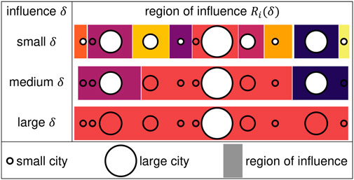
FIGURE 1. Scheme for constructing the region of influence ${\mathcal{R}}_i(\delta )$ of cities. Cities are represented by discs, according to their size. For a short influence distance δ (top) many small regions are formed, represented by different colour ribbons. The centre of each region is the white disc. Some of the cities which were a centre for small values of the influence distance δ, become part of the region of influence of another city for larger values of δ.

For different values of δ, a distinct number of regions of influence is obtained, that is, M depends on δ. Also, a region of influence ${\mathcal{R}}_i(\delta )$ might contain a single city (for instance, for isolated towns and/or small values of δ).

For each region of influence, two metrics are constructed. First, the number of cities κ_i(δ) > 0, corresponding to the number of cities in ${\mathcal{R}}_i(\delta )$ including city i. Second, the population of influence ϕ_i(δ) ≥ 0, corresponding to the urban population inside region ${\mathcal{R}}_i(\delta )$, but now without considering the population of city C_i. By not counting the population of city C_i, then a large value for ϕ_i(δ) is not due to a large population in C_i directly.

2.2 Comparing Against Randomness

The algorithm for constructing regions of influence is based on city size. Therefore, regions of influence with larger centres will be more likely to have higher values of κ_i(δ) and of ϕ_i(δ) since they appear early on in the list. Thus, observing any impact of city size could be simply the result of the algorithm and not because large cities are surrounded by more emergent cities and more population.

To detect if the observed results are only due to our algorithm or if large cities are, in fact, surrounded by more emergent cities and population, we consider a random permutation of the nodes in the network as follows. We keep the structure of nodes and edges, but we permute the city size among its nodes. With this technique, a large city takes up a random location in the network. We then follow the same algorithm to construct regions of influence and measure a permuted (p) number of cities ${\kappa }_i^{(p)}(\delta )$ and the population of influence ${\varphi }_i^{(p)}(\delta )$. Suppose the results observed for the original network and the permuted network for κ_i(δ) and ${\kappa }_i^{(p)}(\delta )$, and also in terms of the population ϕ_i(δ) and ${\varphi }_i^{(p)}(\delta )$ are similar. In this case, the metrics are the result of our algorithm. However, if the observed metrics are different when the network is permuted, we can ensure that large cities’ position in the network creates this observed urban scaling.

3 Results

Useful insights arise when observing Africa’s urban network. For example, defining the city degree as the number of roads that connect it with somewhere else (so, the city degree is the node degree), a sublinear behaviour is observed [55]. The road network made of continental cities in Africa has a diameter (or maximum network distance) of 11,950 km between Umtata Central in South Africa and Tinduf in Argelia. The average road distance between each pair of cities is 4,559 km. In contrast, the average geodesic distance is 3,264 km, suggesting that road distances are 39.6% times larger than the shortest distance between cities (Figure 2).

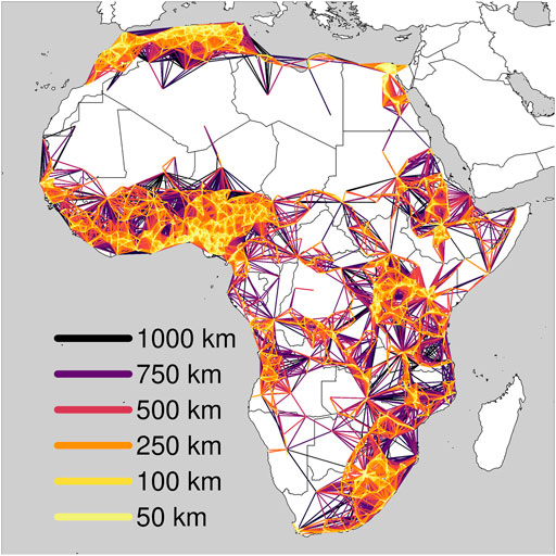
FIGURE 2. For different values of δ, distinct regions of influence are constructed. For some value of δ, all regions of influence are identified using the same colour. Larger values of δ have darker colours and smaller values of δ, corresponding to smaller regions of influence, have lighter colours.

The network has 2,162 cities. With δ = 50 km, we get M = 1, 131 regions of influence (Figure 3). However, by simulating 2,162 random points inside continental Africa and following the same procedure (also with δ = 50 km), we obtain 1, 680 ± 25 regions. Therefore, cities are much more clustered than randomness would suggest, and there are vast empty regions in the continent (Figure 2). Also, we observe that the most isolated town in the continent is in the south of Libya, in the Sahara Desert, 851 km away from the nearest city. However, by simulating 2,162 random points inside Africa, we get that the most isolated town is roughly 200 km away from the nearest city. Indeed, most cities are clustered around some main urban corridors (including the Nile River, the Mediterranean coast, the Lagos-Abidjan coast in West Africa, Lake Victoria and the South Africa network). Still, some cities are highly isolated in the Sahara Desert, the Congolian Rainforest and the Kalahari Desert in Botswana, Namibia and South Africa (see the Supplementary Appendix).

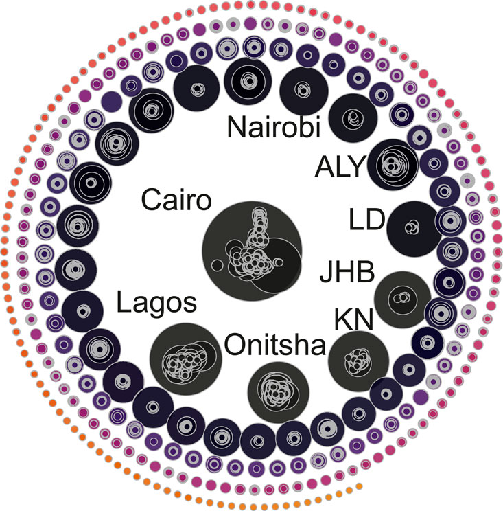
FIGURE 3. The result of considering δ = 255 km. The procedure gives M = 288 regions of influence. The largest region of influence has 246 cities and 57 million inhabitants, with Cairo at its centre. The largest centres are Cairo, Lagos, Onitsha, Kinshasa, Johannesburg, Luanda, Alexandria and Nairobi. With δ = 255 km, there are 84 regions of influence with a single city.

With a distance δ = 70 km, the largest region of influence has Cairo as its centre, with 40.3 million inhabitants (57% of them corresponding to people living in Cairo and 43% in cities nearby Cairo).

3.1 Impact of City Size on the Regions of Influence

For some value of δ, the expected number of cities inside a region of influence conditional on the population size of the centre P_i is denoted by E[κ_i|P_i]. We use the urban scaling modelling framework to express this quantity according to Eq. 2:

where α_δ and β_δ are the scaling coefficients corresponding to the quantity κ_i(δ). We estimate the value of these scaling coefficients via a Poisson regression. For example, for a distance δ = 155 km, we get that α₁₅₅ = (7.326 ± 1.262) × 10^–4 and that β₁₅₅ = 0.682 9 ± 0.012, so the expected number of cities inside a region of influence is given by $E[{\kappa }_i(\delta )|P_i]=7.326P_i^{0.6829}\times 10^{-4}$. We also use the same procedure to model the expected population of the region of influence, conditional on the population of the centre. This can be expressed as

for some a_δ and b_δ which are the scaling coefficients for ϕ_i(δ). Again, a Poisson regression yields for δ = 155 km, a₁₅₅ = 0.567 3 ± 0.000 4 and b₁₅₅ = 1.022 ± 5 × 10^–5. For δ = 155 km, our results suggest that regions of influence where the centre is a large city have more urban agglomerations and more population than regions where the centre is smaller (Figure 4).

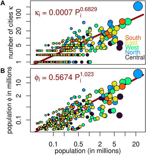
FIGURE 4. Number of cities κ(155) inside regions of influence (A) and population inside the region of influence (ignoring the population from the centre) ϕ(155) (B) against city size (horizontal axis). Axis have a logarithmic scale. Each city is represented by a coloured disc, with its size proportional to population. Five African regions are represented by the colour of the disc.

For values of δ = 155 we get that β₁₅₅ is smaller than one and b₁₅₅ is close to one. Yet, the impact of city size is significant for the size and population of regions of influence. Comparing, for example, the number of cities of the region of influence of city C_i and of city C_j, ten times larger than city C_i, then we expect ${\alpha }_{155}{P}_j^{{\beta }_{155}}/{\alpha }_{155}{P}_i^{{\beta }_{155}}=10^{{\beta }_{155}}\approx 4.8$ times more cities and $10^{b_{155}}\approx 10.5$ times more population (without considering the population from the centre). Furthermore, this is not the result of constructing regions of influence based on larger cities. By permuting the population of cities in the network, we get that ${\beta }_{155}^{(p)}\in (0.496\mathrm{8,0.570}2)$, which is far from the observed value of β₁₅₅ = 0.682 9 ± 0.012, and $b_{155}^{(p)}\in (0.701\mathrm{0,0.890}7)$, also far from the b₁₅₅ = 1.022 ± 5 × 10^–5 obtained.

How far the region of influence of a city spreads is a critical aspect of the model. By considering different values of the influence distance δ, we obtain different regions of influence. The result also gives different values for β_δ and b_δ (Figure 5).

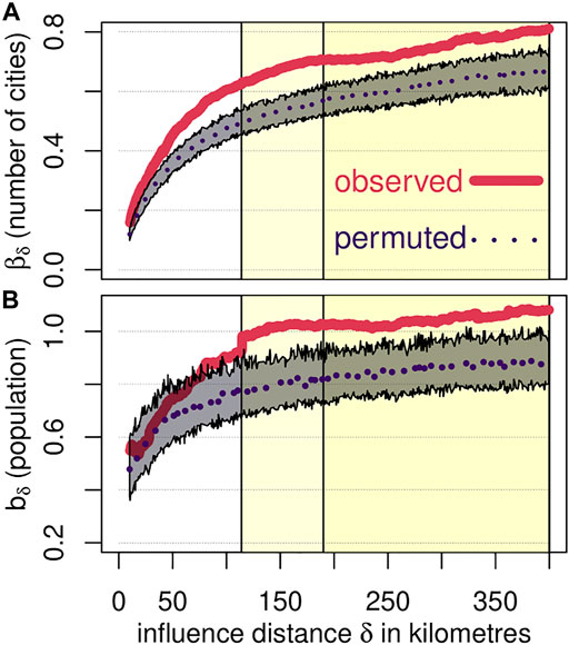
FIGURE 5. Observed and permuted values of β_δ (A) and b_δ (B) for the number of cities and the population in the region of influence of cities. The horizontal axis is the influence distance δ in kilometres. The red lines are the observed values, and the purple line and the shaded interval around the permuted results give the range of values obtained from the permuted network. Intervals are obtained for a fixed value of δ by permuting 100 times the population size of cities and removing the top 5 and the bottom 5 simulated values to drop outliers.

The observed scaling parameters for the number of cities β_δ remain above and outside the intervals obtained with a permuted network. Thus, the number of cities inside a region of influence grows with city size in a non-trivial manner. Therefore, the network structure plays a role, and large cities tend to be surrounded by numerous urban agglomerations. The observed scaling parameter for the urban population within a region of influence b_δ also remains above the permuted values. However, for small distances, it has values inside the interval of the permuted network, suggesting that cities tend to be surrounded by smaller towns rather than big cities.

For small regions of influence, we get many cites with a small population. For example, for δ = 50 km, we get that β₅₀ = 0.3. Thus, when a city is ten times larger, it has twice as many cities within a network distance of 50 km (since 10^0.3 ≈ 2). For the same δ = 50 km, b₅₀ = 0.56. When a city is ten times larger, it has 3.6 times more population within a distance of 50 km. Thus, a ten times larger city tends to have twice as many urban areas and 3.6 times more population at a distance of 50 km. Meaning it has more and larger cities nearby.

The average size of cities within the region of influence depends on the population of the centre which can be computed based on Eq. 2. The result gives

where the exponent (b_δ − β_δ) > 0 indicates that large cities are surrounded by more populous urban agglomerations. Results show that b_δ − β_δ remains well above values of zero for all values of δ > 0 (Figure 6).

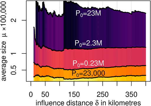
FIGURE 6. Average city size (vertical axis) for different values of the influence distance δ (horizontal axis) for a centre with a population of 23 million inhabitants (nearly the population of Cairo, for example) in purple, and a city 10, 100, and 1000 times smaller (the pink, orange, and yellow polygons). Thus, at a distance of 50 km from a city with the size of Cairo, for example, we expect cities to have an average size of roughly 300,000 inhabitants. However, at a distance of 50 km from a smaller city, for example, a centre with 2.3 million inhabitants, cities in the region of influence will have, on average, 100,000 inhabitants.

Our results indicate that big cities are surrounded by more and larger cities within their region of influence. The result is not due to the construction of regions of influence since the permuted network gives less significant coefficients. Large cities tend to cluster, whereas small cities are more likely to be isolated [64]. Cities form hierarchical structures, a pattern that has also been observed for roads [65].

There is a significant difference between the size at the centre and the size of cities within the region of influence. Only a few cities are large, and most are small [30]. For example, for Cairo (with nearly 23 million inhabitants), the average size of a city in its region of influence is 300,000 inhabitants within a few kilometres, and it decays with distance to 200,000. After a discontinuity at about 114 km from the centre, the size increases slightly to 260,000 but then decays again with more considerable distances (Figure 6). Thus, cities the size of Cairo, Lagos or Johannesburg can be thought of as massive planets surrounded by a surprisingly large number of minor satellites orbiting around. Considering a network distance of δ = 155 km, for example, Cairo has 215 cities within its region of influence, with an average size of fewer than 150,000 inhabitants in each satellite town. Although minor in size, the 215 satellite towns have a total population of 31 million inhabitants, thus, surpassing the size of Cairo itself. Within 155 km of Cairo, the city is only 43% of the urban population of the region of influence. This region of influence is similar to the Alexandria-Cairo-Luxor mega-city constructed based on clustering distinct agglomerations [40]. And the same goes for Lagos, with 49 satellite towns adding nearly 13 million inhabitants in the region. Within 155 km, ten out of the top twenty most populated cities in Africa have less than 60% of the population of their regions of influence.

3.2 Regions With High Isolation

Scaling studies often focus on the large cities, but on the other side of the spectrum, we find a high level of isolation with huge distances to some primary city. Isolation is one of the main contributors to poverty [66] and our results show that some cities are highly isolated.

For example, with δ = 155 km, results show that 203 regions of influence are formed of a single city, with an average size of 90,000 inhabitants. In total, 18.6 million people live in a city that is a single city within a region of influence. Still, with δ = 155 km, we get 406 regions of influence where the total population, considering people from the centre as well, has less than one million inhabitants. This means that 406 regions (with 87 million people combined) with less than one million people living in cities within 155 km. In the extreme case, with δ = 1000 km, we find nine towns at a distance of 1000 km or more to their nearest city. Africa is characterised by large booming cities surrounded by an even larger population nearby and many regions with high isolation.

4 Discussion

Many socio-economic indicators tend to be have disproportionally larger values in more populated cities. For example, large cities tend to have higher crime levels and produce more patents, on a per capita basis (superlinear scaling). Meanwhile, there are other urban indicators, typically those referring to infrastructure, which increase slower than the population (sublinear scaling), suggesting less demand and a sharing of resources. Urban scaling is a crucial aspect of cities that can bring value in the design of policies for producing faster and more sustainable development [67]. Here, we showed that the scaling impact of city size goes beyond urban indicators experienced within the city. Large cities are surrounded by a disproportionate number of urban agglomerations and corresponding populations, and the effect is observed for some distance, even hundreds of kilometres.

Rather than the city coordinates and geodesic distances, a consideration of the urban network offers a more realistic approximation for travel between cities. A network where the cities are nodes and where the road infrastructure are the edges provides significant details regarding city connectivity and existent natural and political barriers. The network might not capture some details at a very small scale, for instance, details at the street level, such as tolls or highways. Also, the network itself might not be needed for very long distances since approximating the road distance by inflating the geodesic distance by a constant factor of 1.396 [55] is sufficiently accurate for measuring long-distance interactions. Thus, after a certain threshold, the road distance grows linearly with the geodesic distance (see the Supplementary Appendix). However, for medium distances (between 20 and 300 km), where intracity interactions are more prevalent, the network captures the infrastructure, political barriers and the fragmentation of the continent, among many factors that increase the road distance of nearby cities, thus, reducing their interactions.

Our method for constructing regions of influence has some caveats. First, the way cities are defined may alter results [38, 68, 69]. Here, we have used an Open Access dataset that combines satellite and aerial imagery, official demographic data such as censuses and other cartographic sources [61]. A city polygon is defined as an area with less than 200 m between buildings and constructions in the data. Results might change if a different definition of a city is adopted. Second, the method ignores the implications of international borders in a continent that is not fully integrated and where borders might impose a high cost on journeys and travel between cities. African border cities are growing faster than the average [70], suggesting that international borders are an essential part of the continent’s dynamics and play a role in urban interactions. Third, a city is assigned to a unique region of influence, but some urban areas might have a high dependence and interactions with many cities, perhaps in a hierarchical manner (see the Supplementary Appendix for the results of constructing regions of influence using a hierarchical algorithm). Fourth, we have assumed the same distance threshold across the whole continent for constructing regions of influence. Thus, we use the same values of δ to construct the region of influence for Nairobi as Cairo, a city four times the size and in a more industrialised country. It is possible to consider other techniques, such as a distance-decay function or varying values of δ depending on city size, for example, by setting $\delta (P_i)=\rho P_i^{\gamma }$, for some values of ρ and γ (so our model is for γ = 0). Also, the impact of distance and the construction of regions of influence may differ in less densely populated and less urban areas. For example, some regional aspects could also be considered. Notice that large cities from the central region of Africa (Figure 4, coloured differently from other regions) fall under the expected number of cities κ and population ϕ within their region of influence. Also, with our scaling parameters, we only observe correlations and not causality for the emergence or the growth of cities. For example, the region along the Nile River and its delta has attracted the emergence of Egyptian cities for its proximity to water but maybe also due to its proximity to Cairo or Alexandria.

Despite those caveats, our results still show some non-trivial patterns in the structure of the urban system formed by African cities. The observed patterns are at the core of serious social issues such as poverty, inequality or isolation.

4.1 Regions of Influence of the Present, Mega-Cities of the Future?

When looking at the current situation of cities, it is as if we are observing a screenshot of a movie that is still playing. Particularly, since the urban scaling models are applied to cross-sectional data, the interpretation of the results obtained here should be used in a comparative or descriptive manner as opposed to a predictive one [71]. Cities are very dynamic and will evolve, grow and adapt [72], and so the values of the scaling parameters computed here are also likely to change. This is especially the case for the population size of African cities. What has happened in some cities in the last 60 years may be nothing compared to what will happen in the next 60 years [73]. In 2020, for example, Egypt was home to 102 million inhabitants, and it is expected to double its population before 2080. The same is true, if not more so, for many African countries, with, for example, Chad, Mali and Niger expected to double their 2020 population before 2050 or even before 2040. Therefore, Ndjamena, Bamako and Niamey will likely double their population in the upcoming decades. If urbanisation and population growth continue, Lagos in Nigeria could soon become the world’s largest city, home to 85 or 100 million people [73].

It is likely that what we observe today as a large metropolis surrounded by dozens of minor satellite urban areas within its region of influence will become a unified polycentric city. A large metropolis will thus incorporate peripheral agglomerations as it expands [74]. Hence, some, if not most of the cities within the region of influence of large metropolitan areas such as Lagos or Kinshasa, probably will eventually merge. Today’s large regions of influence are tomorrow’s polycentric cities.

Data Availability Statement

The original contributions presented in the study are included in the article/Supplementary Material, further inquiries can be directed to the corresponding author.

Author Contributions

RPC designed the study. RPC and CC-A analysed the results. All authors wrote the manuscript.

Funding

RPC received funding for this work from the UKRI’s Global Challenge Research Fund, grant: PES/P011055/1. CC-A received funding for this work from the European Research Council's H2020-EU.1.1. Excellent Science Programme, grant: 949670.

Conflict of Interest

The authors declare that the research was conducted in the absence of any commercial or financial relationships that could be construed as a potential conflict of interest.

Publisher’s Note

All claims expressed in this article are solely those of the authors and do not necessarily represent those of their affiliated organizations, or those of the publisher, the editors and the reviewers. Any product that may be evaluated in this article, or claim that may be made by its manufacturer, is not guaranteed or endorsed by the publisher.

Supplementary Material

The Supplementary Material for this article can be found online at: https://www.frontiersin.org/articles/10.3389/fphy.2022.858307/full#supplementary-material

References

1. Bai X, Surveyer A, Elmqvist T, Gatzweiler FW, Güneralp B, Parnell S, et al. Defining and Advancing a Systems Approach for Sustainable Cities. Curr Opin Environ Sustainability (2016) 23:69–78. doi:10.1016/j.cosust.2016.11.010
2.[Dataset] Population Division of the UN. Department of Economic and Social Affairs. In: UN World Urbanization Prospects: The 2018 Revision (2018).
3. Seto KC, Güneralp B, Hutyra LR. Global Forecasts of Urban Expansion to 2030 and Direct Impacts on Biodiversity and Carbon Pools. Proc Natl Acad Sci (2012) 109:16083–8. doi:10.1073/pnas.1211658109
4. Seto KC, Reenberg A, Boone CG, Fragkias M, Haase D, Langanke T, et al. Urban Land Teleconnections and Sustainability. Proc Natl Acad Sci (2012) 109:7687–92. doi:10.1073/pnas.1117622109
5. Gong P, Liang S, Carlton EJ, Jiang Q, Wu J, Wang L, et al. Urbanisation and Health in China. The Lancet (2012) 379:843–52. doi:10.1016/S0140-6736(11)61878-3
6. Combes P, Duranton G, Gobillon L, Puga D, Roux S. The Productivity Advantages of Large Cities: Distinguishing Agglomeration from Firm Selection. Econometrica (2012) 80:2543–94. doi:10.3982/ECTA8442
9. Winters JV. Why Are Smart Cities Growing? Who Moves and Who Stays*. J Reg Sci (2011) 51:253–70. doi:10.1111/j.1467-9787.2010.00693.x
10. Angel S, Sheppard C, Civco D, Buckley P, Chabaeva A, Gitlin L, et al. The Dynamics of Global Urban Expansion. Washington, DC: Transport and Urban Development Department, The World Bank (2005).
11. Ericksen PJ. Conceptualizing Food Systems for Global Environmental Change Research. Glob Environ Change (2008) 18:234–45. doi:10.1016/j.gloenvcha.2007.09.002
12. Parr J. Perspectives on the City‐region. Reg Stud (2005) 39:555–66. doi:10.1080/00343400500151798
13. Reiner TA, Parr JB. A Note on the Dimensions of a National Settlement Pattern. Urban Stud (1980) 17:223–30. doi:10.1080/00420988020080381
14. Pumain D. Settlement Systems in the Evolution. Geografiska Annaler: Ser B, Hum Geogr (2000) 82:73–87. doi:10.1111/j.0435-3684.2000.00075.x
15. Barthelemy M. The Statistical Physics of Cities. Nat Rev Phys (2019) 1:406–15. doi:10.1038/s42254-019-0054-2
16. Batty M. The Size, Scale, and Shape of Cities. Science (2008) 319:769–71. doi:10.1126/science.1151419
17. Bettencourt LMA, Lobo J, Strumsky D, West GB. Urban Scaling and its Deviations: Revealing the Structure of Wealth, Innovation and Crime across Cities. PLoS One (2010) 5:e13541. doi:10.1371/journal.pone.0013541
18. Haldane J, Haldane JBS. In: JM Smith, editor. Oxford Paperbacks (1985).On Being the Right Size and Other Essays /
20. Glaeser EL, Sacerdote B. Why Is There More Crime in Cities? J Polit Economy (1999) 107:S225–S258. doi:10.1086/250109
21. Fragkias M, Lobo J, Strumsky D, Seto KC. Does Size Matter? Scaling of CO2 Emissions and U.S. Urban Areas. PLOS ONE (2013) 8:e64727–8. doi:10.1371/journal.pone.0064727
22. Schläpfer M, Bettencourt LMA, Grauwin S, Raschke M, Claxton R, Smoreda Z, et al. The Scaling of Human Interactions with City Size. J R Soc Interf (2014) 11:20130789. doi:10.1098/rsif.2013.0789
23. Youn H, Bettencourt LMA, Lobo J, Strumsky D, Samaniego H, West GB. Scaling and Universality in Urban Economic Diversification. J R Soc Interf (2016) 13:20150937. doi:10.1098/rsif.2015.0937
24. Strano E, Giometto A, Shai S, Bertuzzo E, Mucha PJ, Rinaldo A. The Scaling Structure of the Global Road Network. R Soc Open Sci (2017) 4:170590. doi:10.1098/rsos.170590
25. Prieto Curiel R, Pappalardo L, Gabrielli L, Bishop SR. Gravity and Scaling Laws of City to City Migration. PloS one (2018) 13:e0199892. doi:10.1371/journal.pone.0199892
26. Prieto Curiel R, Cabrera Arnau C, Torres Pinedo M, González Ramírez H, Bishop SR. Temporal and Spatial Analysis of the media Spotlight. Comput Environ Urban Syst (2019) 75:254–63. doi:10.1016/j.compenvurbsys.2019.02.004
27. Cabrera-Arnau C, Prieto Curiel R, Bishop SR. Uncovering the Behaviour of Road Accidents in Urban Areas. R Soc Open Sci (2020) 7:191739. doi:10.1098/rsos.191739
28. Cabrera-Arnau C, Bishop SR. Urban Population Size and Road Traffic Collisions in Europe. PLOS ONE (2021) 16:e0256485–13. doi:10.1371/journal.pone.0256485
31. Steindl J. Random Processes and the Growth of Firms. New York, NY: A Study of the Pareto Law Hafner (1965).
32. Simon HA. On a Class of Skew Distribution Functions. Biometrika (1955) 42:425–40. doi:10.1093/biomet/42.3-4.425
34. Cottineau C. Metazipf. A Dynamic Meta-Analysis of City Size Distributions. PLOS ONE (2017) 12:e0183919–22. doi:10.1371/journal.pone.0183919
36. Puga D. The Magnitude and Causes of Agglomeration Economies. J Reg Sci (2010) 50:203–19. doi:10.1111/j.1467-9787.2009.00657.x
37. Scott AJ. The Cultural Economy of Cities. Int J Urban Reg Res (1997) 21:323–39. doi:10.1111/1468-2427.00075
38. Rozenfeld HD, Rybski D, Andrade JS, Batty M, Stanley HE, Makse HA. Laws of Population Growth. Proc Natl Acad Sci (2008) 105:18702–7. doi:10.1073/pnas.0807435105
39. Fluschnik T, Kriewald S, García Cantú Ros A, Zhou B, Reusser D, Kropp J, et al. The Size Distribution, Scaling Properties and Spatial Organization of Urban Clusters: a Global and Regional Percolation Perspective. Ijgi (2016) 5:110. doi:10.3390/ijgi5070110
40. Oliveira EA, Furtado V, Andrade JS, Makse HA. A Worldwide Model for Boundaries of Urban Settlements. R Soc Open Sci (2018) 5: 180468. doi:10.1098/rsos.180468
41. Duranton G. Delineating Metropolitan Areas: Measuring Spatial Labour Market Networks through Commuting Patterns. In: The Economics of Interfirm Networks. Springer (2015). p. 107–33. doi:10.1007/978-4-431-55390-8_6
43. Neal ZP. The Connected City: How Networks Are Shaping the Modern metropolis. New York, USA: Routledge (2012).
44. van Meeteren M. About Being in the Middle: Conceptions, Models and Theories of Centrality in Urban Studies. In Handbook of Cities and Networks. Edward Elgar Publishing (2021). p. 672. doi:10.4337/9781788114714.00019
45. Lei W, Jiao L, Xu Z, Zhou Z, Xu G. Scaling of Urban Economic Outputs: Insights Both from Urban Population Size and Population Mobility. Comput Environ Urban Syst (2021) 88:101657. doi:10.1016/j.compenvurbsys.2021.101657
46. Pitts FR. A Graph Theoretic Approach to Historical Geography. The Prof Geographer (1965) 17:15–20. doi:10.1111/j.0033-0124.1965.015_m.x
47. Chan SH, Donner RV, Lämmer S. Urban Street Networks as an Example for Spatial Networks with Universal Geometric Features: A Case Study from Germany. EGU General Assembly Conference Abstracts (2010). p. 13522.
48. Van Meeteren M, Boussauw K, Derudder B, Witlox F. Flemish diamond or ABC-Axis? the Spatial Structure of the Belgian Metropolitan Area. Eur Plann Stud (2016) 24:974–95. doi:10.1080/09654313.2016.1139058
49. Taylor PJ, Catalano G, Walker DRF. Measurement of the World City Network. Urban Stud (2002) 39:2367–76. doi:10.1080/00420980220080011
50. Nystuen JD, Dacey MF. A Graph Theory Interpretation of Nodal Regions. Pap Reg Sci Assoc (1961) 7:29–42. doi:10.1007/bf01969070
51. Wiedermann M, Donges JF, Kurths J, Donner RV. Spatial Network Surrogates for Disentangling Complex System Structure from Spatial Embedding of Nodes. Phys Rev E (2016) 93:042308. doi:10.1103/PhysRevE.93.042308
52. Louf R, Jensen P, Barthelemy M. Emergence of Hierarchy in Cost-Driven Growth of Spatial Networks. Proc Natl Acad Sci (2013) 110:8824–9. doi:10.1073/pnas.1222441110
53. Gastner MT, Newman MEJ. The Spatial Structure of Networks. Eur Phys J B (2006) 49:247–52. doi:10.1140/epjb/e2006-00046-8
54. Dupuy G, Stransky V. Cities and Highway Networks in Europe. J Transport Geogr (1996) 4:107–21. doi:10.1016/0966-6923(96)00004-x
55. Prieto Curiel R, Schumann A, Heo I, Heinrigs P. Detecting Cities with High Intermediacy in the African Urban Network (2021). arXiv e-prints arXiv–2110.
56. Linard C, Tatem AJ, Gilbert M. Modelling Spatial Patterns of Urban Growth in Africa. Appl Geogr (2013) 44:23–32. doi:10.1016/j.apgeog.2013.07.009
58. Meijers EJ, Burger MJ, Hoogerbrugge MM. Borrowing Size in Networks of Cities: City Size, Network Connectivity and Metropolitan Functions in Europe. Pap Reg Sci (2016) 95:181–98. doi:10.1111/pirs.12181
59. Linard C, Gilbert M, Snow RW, Noor AM, Tatem AJ. Population Distribution, Settlement Patterns and Accessibility across Africa in 2010. PLoS One (2012) 7:e31743. doi:10.1371/journal.pone.0031743
60. Poletti P, Parlamento S, Fayyisaa T, Feyyiss R, Lusiani M, Tsegaye A, et al. The Hidden burden of Measles in Ethiopia: How Distance to Hospital Shapes the Disease Mortality Rate. BMC Med (2018) 16:177. doi:10.1186/s12916-018-1171-y
61. [Dataset] Moriconi-Ebrard F, Harre D, Heinrigs P. Urbanisation Dynamics in West Africa 1950–2010 (2015). http: //dx.doi.org/10.1787/9789264252233-en.
62.[Dataset] OpenStreetMap contributors. Planet Dump Retrieved from (2021). Available at: https://www.openstreetmap.org. (Accessed November, 2021)
63. Ioannides YM, Overman HG. Spatial Evolution of the US Urban System. J Econ Geogr (2004) 4:131–56. doi:10.1093/jeg/4.2.131
64. Mansury Y, Shin JK. Size, Connectivity, and Tipping in Spatial Networks: Theory and Empirics. Comput Environ Urban Syst (2015) 54:428–37. doi:10.1016/j.compenvurbsys.2015.08.004
65. Lämmer S, Gehlsen B, Helbing D. Scaling Laws in the Spatial Structure of Urban Road Networks. Physica A: Stat Mech its Appl (2006) 363:89–95. doi:10.1016/j.physa.2006.01.051
66. Linard C, Gilbert M, Snow RW, Noor AM, Tatem AJ. Population Distribution, Settlement Patterns and Accessibility across Africa in 2010. PLoS One (2012) 7:e31743. doi:10.1371/journal.pone.0031743
67. Bettencourt LMA, Lobo J, Helbing D, Kühnert C, West GB. Growth, Innovation, Scaling, and the Pace of Life in Cities. Proc Natl Acad Sci (2007) 104:7301–6. doi:10.1073/pnas.0610172104
68. Arcaute E, Youn H, Ferguson P, Hatna E, Batty M, Johansson A. City Boundaries and the Universality of Scaling Laws. ArXiv (2013).
69. Oliveira EA, Andrade JS, Makse HA. Large Cities Are Less green. Sci Rep (2014) 4:4235. doi:10.1038/srep04235
70.OECD. Population and Morphology of Border Cities. Paris: Organisation for Economic Cooperation and Development, Sahel and West Africa Club (2019). doi:10.1787/80dfd9d8-en
71. Bettencourt LMA, Yang VC, Lobo J, Kempes CP, Rybski D, Hamilton MJ. The Interpretation of Urban Scaling Analysis in Time. J R Soc Interf (2020) 17:20190846. doi:10.1098/rsif.2019.0846
72. Parnell S, Elmqvist T, McPhearson T, Nagendra H, Sörlin S. Introduction: Situating Knowledge and Action for an Urban planetThe Urban Planet: Knowledge towards Sustainable Cities. Cambridge: Cambridge University Press (2018). p. 1–16. doi:10.1017/9781316647554.002
73. Hoornweg D, Pope K. Population Predictions for the World's Largest Cities in the 21st century. Environ Urbanization (2017) 29:195–216. doi:10.1177/0956247816663557
Keywords: scaling, urban network, Africa, city size, emergence, growth
Citation: Prieto Curiel R, Cabrera-Arnau C and Bishop SR (2022) Scaling Beyond Cities. Front. Phys. 10:858307. doi: 10.3389/fphy.2022.858307
Received: 19 January 2022; Accepted: 28 February 2022;
Published: 05 April 2022.
Edited by:
Haroldo V. Ribeiro, State University of Maringá, BrazilReviewed by:
Hygor Piaget Monteiro Melo, University of Lisbon, PortugalErneson Oliveira, University of Fortaleza, Brazil
Copyright © 2022 Prieto Curiel, Cabrera-Arnau and Bishop. This is an open-access article distributed under the terms of the Creative Commons Attribution License (CC BY). The use, distribution or reproduction in other forums is permitted, provided the original author(s) and the copyright owner(s) are credited and that the original publication in this journal is cited, in accordance with accepted academic practice. No use, distribution or reproduction is permitted which does not comply with these terms.
*Correspondence: Carmen Cabrera-Arnau, c.cabrera-arnau@ucl.ac.uk