The Metastable Mpemba Effect Corresponds to a Non-monotonic Temperature Dependence of Extractable Work

1. Introduction

A generic consequence of the second law of thermodynamics is that a system, once perturbed, will tend to relax back to thermal equilibrium. Such relaxation is typically exponential. To understand why, consider energy relaxation and recall that the heat equation,

for the temperature field T at position r and time t and thermal diffusivity κ has solutions that can be written in the form¹

Here, T_∞(r) is the static temperature-field solution of Equation (1); it must account for boundary conditions. For t → ∞, an arbitrary initial condition T(r, 0) will relax to this state. In Equation (2), the v_m(r) are spatial eigenfunctions, with corresponding eigenvalues λ_m and coefficients a_m, which represent the projections of the field [T(r, 0) − T_∞(r)] onto the corresponding eigenfunction. For long but finite times, all but the slowest eigenmode will have decayed, and the temperature is, approximately,

which, indeed, shows a simple exponential decay to T_∞(r) for a probe at a fixed position r.

Although exponential decays are typical, anomalous, non-exponential relaxation is also encountered. Large objects, for example, may have an asymptotic time scale ${\lambda }_2^{-1}$ that exceeds experimental times, so that it is not possible to wait “long enough.” Similarly, glassy systems and other complex materials may have a spectrum of exponents for mechanical and dielectric relaxation that have not only very long time scales but also many closely spaced values that are not resolved as a sequence of exponentials. Rather, they can collectively combine to approximate a power-law or even logarithmic time decay, with specific details that depend on the history of preparation [2].

Another class of anomalous systems shows unexpectedly fast relaxation in certain circumstances. The best-known of these is the observation that, occasionally, a sample of hot water may cool and begin to freeze more quickly than a sample of cool or warm water prepared under identical conditions. Based on the scenario of exponential relaxation sketched above, one's naive intuition is that a hotter system will have to “pass through” all intermediate temperatures and thus take longer to equilibrate. More succinctly, the observation is that, in some systems, the equilibration time is a non-monotonic function of the initial temperature: the time for a system initially in equilibrium at a given temperature takes to cool and reach equilibrium with the bath temperature does not always increase with initial temperature.

While observations of this phenomenon date back two millennia to the ancient Greeks [3, 4], its modern study began with observations by Mpemba in the 1960s [5]. The effect has since been observed in systems such as manganites [6], clathrates [7], polymers [8, 9], and predicted in simulations of other systems, including carbon nanotube resonators [10], granular fluids [11], and spin glasses [12]. In all these Mpemba effects, the relaxation time shows a surprisingly complicated dependence on the deviation of initial temperature from equilibrium: increasing and then decreasing, and in some cases increasing again with increasing deviation. The relaxation time thus does not increase monotonically with the deviation from equilibrium, as one might naively expect.

One challenge in studying Mpemba effects is that the systems where they have been observed or predicted have been rather complicated, with many possible explanations for the effect. The explanations tend to be complicated and specific to a particular system. Even water is not as simple as it might seem: proposed mechanisms include evaporation [13–15], convection [16], supercooling [17], dissolved gases [18], and effects arising from hydrogen bonds [19].

In an effort to understand the Mpemba effect more generically, Lu and Raz recently proposed an explanation that is linked to the structure of eigenfunction expansions such as that in Equation (2) [1]. Their work was formulated for mesoscopic systems that are in the classical regime yet are small enough that thermal fluctuations make an important contribution to their dynamics. Such systems may be described by master equations and Fokker-Planck equations, for finite and continuous state spaces, respectively [20–24]. For the latter, the Fokker-Planck equation describes the evolution of the probability density function p(x, t) for a system described by a state vector x(t)². Its structure is similar to that of Equation (1): its linearity implies that solutions are also described by an infinite-series, eigenfunction expansion similar to that in Equation (2). The essence of Lu and Raz's explanation is that the projection of the initial state p(x, 0)—a Gibbs-Boltzmann distribution corresponding to an initial temperature T—onto the slowest eigenfunction, a₂ can be non-monotonic in T, or, equivalently, in ${\beta }^{-1}\equiv k_{\text{B}}T$, where k_B ≡ 1 (in our units) is Boltzmann's constant. Such a consequence implies a Mpemba effect because the long-time limit for the probability density function has the same form as Equation (3):

with g_βb(x) the Gibbs-Boltzmann distribution for the system at a temperature T_b corresponding to the surrounding thermal bath with which the system is in contact and can exchange energy. Equation (4) is valid after an initial transient time $\approx {\lambda }_3^{-1}$. The coefficient a₂ is a function of both the initial temperature and bath temperature:

where the initial state p(x, 0) is assumed to be in equilibrium at a higher temperature β⁻¹ and where u_2,βb(x) is the left eigenfunction of the Fokker-Planck operator, which is the dual-basis element corresponding to the right eigenfunction v_2,βb(x) of the same Fokker-Planck operator. Both u₂ and v₂ are calculated for the Markovian Langevin dynamics associated with white noise whose covariance is set by the bath temperature, ${\beta }_{\text{b}}^{-1}$. We need to distinguish between left and right eigenfunctions because the operator generating Fokker-Planck dynamics is not self-adjoint, in contrast to the operator generating the heat-diffusion dynamics discussed in Equation (1). The Mpemba effect then translates to the non-monotonicity of a₂ as a function of the initial temperature β⁻¹: If a high-temperature initial condition has a smaller coefficient a₂, then, in the long-time limit, the system will be closer to equilibrium than a cool-temperature initial condition with larger a₂. This non-monotonicity in a₂ is easier to establish than the non-monotonicity of equilibration times that defines the Mpemba effect. The latter requires either an experiment or, at the very least, repeated numerical solution of the full Fokker-Planck equation.

Inspired by the scenario proposed by Lu and Raz [1], we have explored the Mpemba effect in a simple, mesoscopic setting that—unlike previous work—lends itself to quantitative experiments that straightforwardly connect with theory [25]. In particular, we explored the motion of a single micron-scale colloidal particle immersed in water and moving in a tilted double-well potential. The one-dimensional (1D) state space consists of the position x(t) of the particle. By choosing carefully the tilt of the potential, along with the energy-barrier height and the offset (asymmetry) of the double-well potential within a box that confines the particle motion at high temperatures, we could demonstrate convincingly the existence of the Mpemba effect and measure the non-monotonic temperature dependence of the a₂ coefficient. We even found conditions where a₂ = 0. At such a point, the slowest relaxation dynamics is $~e^{-{\lambda }_{3}t}$, implying an exponential speed-up over the generic relaxation dynamics, $~e^{-{\lambda }_{2}t}$. This strong Mpemba effect had been predicted by Klich et al. [26].

Although our recent experimental work gives strong support to the basic scenario proposed by Lu and Raz, it does not offer good physical insight into the conditions needed to produce or observe the Mpemba effect. What physical picture corresponds to the anomalous temperature dependence of the a₂ coefficient? In this Brief Research Report, we offer a more physical interpretation of the Mpemba effect explored in our previous work.

2. Thermalization in a Double-Well Potential With Metastability

A common feature of experiments showing Mpemba effects is that they involve a temperature quench: the system is cooled very rapidly. We model this situation by making the high-temperature initial state an initial condition for dynamics that take place entirely in contact with a bath of fixed temperature. In effect, the quench is infinitely fast. The overdamped thermalization dynamics are then described by the Langevin equation

with γ a friction coefficient and η(t) Gaussian white noise modeling thermal fluctuations from the bath, with 〈η(t)〉 = 0 and 〈η(t)η(t′)〉 = δ(t − t′). The noise-strength $2\gamma {\beta }_{\text{b}}^{-1}$ enforces the fluctuation-dissipation relation [21, 23]. The potential U(x) is a double-well potential with barrier height $E_0\gg {{\beta }_{\text{b}}}^{-1}$ and two coarse-grained states, denoted L and R in Figure 1A. The range of particle motions is also constrained to a finite range; the potential is implicitly infinite at the extremities. By tilting the potential, one state has a higher energy than the other (difference is ΔE) and becomes a toy model for the water-ice phase transition. However, the energy barrier E₀, while high enough that the two states are well defined, is also low enough that many transitions over the barrier are observed during a typical experiment.

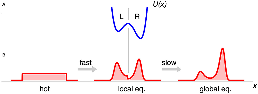
Figure 1. Two-stage dynamics. (A) Tilted double-well potential U(x) with coarse-grained states {L, R}. The potential includes a box (not shown). (B) Evolution of the probability density function for position: a high-temperature equilibrium initial state g_β(x) (left) has a fast relaxation to a local equilibrium state ${\rho }_{\beta ,{\beta }_{\text{b}}}^{\text{leq}}(x)$ (middle) and a slow relaxation to global equilibrium g_βb(x) at the colder bath temperature (right).

Figure 1 illustrates the case studied by Kumar and Bechhoefer [25], with (a) showing the potential and (b) the dynamics of a quench from a high temperature. With a moderately high barrier, both wells have significant probability for the equilibrium state g_βb(x) (Figure 1B, right). For U(x), the barrier E₀ = 2.0, the energy difference between states is ΔE = 1.3, and the hot temperature ${\beta }_{\text{h}}^{-1}=1,000$; all quantities are multiplied by β_b and are, hence, dimensionless. The separation between wells was 80 nm.

At a temperature corresponding to β⁻¹, the equilibrium free energy of the system is

and the corresponding equilibrium Gibbs density is

The metastability of U means that the system evolves on two very different time scales:

Stage 1 is a fast relaxation to local equilibration. The initial, high-temperature Gibbs density rapidly evolves to a state that is at local equilibrium with respect to the bath temperature. A local equilibrium is a density that is similar locally to g_βb, but with altered fractions of systems in the left or right wells. Using marginalization and the definition of conditional probability, we can write such a local-equilibrium state as

More precisely, the local β, β_b equilibrium is the density

with 0 ≤ a_L ≤ 1. Choosing a_L + a_R = 1 ensures normalization of the probability density.

In a fast quench, we assume that the fraction of initial systems at equilibrium at the higher temperature β⁻¹ is unchanged when local equilibrium is established. Essentially, we ignore the diffusion of trajectories that start on one side of the barrier and end up on the other at the end of the transient. In this approximation, the fraction that ends up in each well corresponds to that of the initial state, g_β. Thus,

As shown in Figure 1B, center, the local-equilibrium distribution ${\rho }_{\beta ,{\beta }_{\text{b}}}^{\text{leq}}(x)$ is discontinuous at x = 0; higher barriers will reduce the discontinuity, of order $e^{-{\beta }_{\text{b}}{E}_0}\ll 1$.

Stage 2 is a final relaxation to global equilibrium on a slow time scale: the overall populations in each well (coarse-grained state) change, and the density converge to the Gibbs density g_βb. Local equilibrium is maintained during the evolution, which is illustrated schematically in Figure 1B. In this metastable regime, the equilibration time was analyzed by Kramers long ago [21, 27–29]. It also corresponds to the limit of Equation (4); as a result, the final relaxation is exponential, with decay rate λ₂. Since the duration of Stage 1 is determined by λ₃ and that of Stage 2 by λ₂, time-scale separation between the two stages amounts to the assertion that λ₃/λ₂≫1. In the experiments of [25] revisited here, λ₃/λ₂ ≈ 16.

3. Metastable Mpemba Effect

Given this scenario of thermal relaxation as a two-stage process, we can readily understand how the Mpemba effect can occur. The idea is to follow the dynamics in the function space of all admissible probability density functions p(x, t). If we expand the solution in eigenfunctions analogously to Equation (2), we see that the infinite-dimensional function space is spanned by the eigenfunctions. To visualize the motion, we project it onto the 2D subspace spanned by the eigenfunctions v₂(x) and v₃(x). The system state is then characterized as a parametric plot of the amplitudes a₂(t) and a₃(t). Animations from a 3D projection spanning a₂–a₃–a₄ are available in the Supplementary Material. A similar geometric plot was used to explore quenching in an anti-ferromagnetic Ising spin system in Klich et al. [26].

Figure 2A shows a two-dimensional projection of the geometry of trajectories. They are organized about two static, 1D curves, labeled G, and G_leq. The red curve (G) represents the set of all equilibrium Gibbs-Boltzmann densities, g_β, for 0 ≤ β < ∞. It is sometimes known as the quasi-static locus. The green curve (G_leq) represents the set of all local-equilibrium densities of the form of Equation (9), as parameterized by a_L ∈ [0, 1]. Both curves are represented as 2D parametric plots but lie in the full infinite-dimensional space. Both G and G_leq have finite length, in general. (The entire length is not shown in the figure.) The two curves intersect at a₂ = a₃ = 0, which describes the global equilibrium g_βb with respect to the bath (large hollow marker with dot). The apparent crossing near a₂ ≈ 0.4 is spurious, as the 3D projections in Figure 2B and the supplement show.

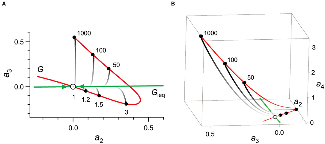
Figure 2. Probability-density dynamics. (A) Two-dimensional dynamics in the plane defined by the a₂ and a₃ coefficients. (B) Three-dimensional dynamics defined by projections onto the a₂, a₃, and a₄ coefficients. In both cases, the red curve G denotes the set of equilibrium densities; the green curve represents G_leq the set of local-equilibrium densities. Arrows indicate the slow relaxation along G_leq to global equilibrium, at the intersection with G (denoted by the large hollow marker with a dot at its center at T = 1). Gray lines denote the rapid relaxation from an initial condition (temperature relative to the bath indicated by a marker along G). The time progression of p(x, t), projected onto the a₂–a₃ plane, is from dark to light. Curves are calculated from the double-well potential described in Kumar and Bechhoefer, with domain asymmetry α = 3 (see [25] for definitions).

The dynamical trajectories are represented by the variously shaded gray curves. At time t = 0, the systems are in equilibrium along the red curve at a variety of temperatures {1, 1.2, 1.5, 3, 50, 100, 1, 000} × T_b, which are indicated by black markers. The curves then move rapidly toward the green curve (local equilibrium). The time course is suggested by the dark-to-light gradient. Once they reach the vicinity of G_leq, they closely follow this green curve back to the global-equilibrium state.

Within this representation, we note the “arrival point” of each trajectory when it “hits” G_leq. For small temperatures (1, 1.2, 1.5, 3), the distance between this arrival point and the global-equilibrium state increases monotonically with β. For larger temperatures (50, 100, 1,000), however, the distance decreases until, at T = 1, 000T_b, it nearly vanishes (denoting the strong Mpemba effect). Along G_leq, the system is in the limit described by Equation (4) and relaxes exponentially to global equilibrium. Relaxation along G_leq therefore must be monotonic with the distance away from global equilibrium. Trajectories that arrive along this curve that are farther from global equilibrium will take longer to relax. In the Appendix, we show that this notion of “distance” along G_leq can be expressed as the Kullback-Leibler divergence D_KL between the local equilibrium density ${\rho }_{\beta ,{\beta }_{\text{b}}}^{\text{leq}}$ given in Equation (9) and the global equilibrium density g_βb. In particular, $D_{\text{KL}}[{\rho }_{\beta ,{\beta }_{\text{b}}}^{\text{leq}},g_{{\beta }_{\text{b}}}]$ is a monotonic function of a_L (defined in Equation 10), which is the natural parameter for the manifold G_leq.

Now we can understand how the (metastable) Mpemba effect can arise. In the example shown in Figure 2, the distance along G_leq initially increases with T and so does the total equilibration time. But then this distance decreases for higher temperatures, leading to the Mpemba effect. We note that in our approximation, the time to traverse the initial stage is much shorter than the time to relax along the green curve, so that variations in the length of the initial trajectory are irrelevant.

If the bath temperature were changed at a finite rate (rather than a hot system being quenched directly into the bath), then the dynamics would be different. For example, if the system is very slowly cooled from the initial temperature to final bath temperature, the trajectory would follow the quasi-static locus (red curve G) and no Mpemba effect would be possible. Having shown that no Mpemba effect is possible with an infinitely slow quench and that the effect can be observed in the limit of an infinitely rapid quench, we can conclude that the Mpemba effect requires a sufficiently fast temperature quench.

4. Metastable Mpemba Effect in Terms of Extractable Work

Our main goal is to express the criterion for the Mpemba effect in more physical terms. For the metastable setting described above, we will find such a criterion in terms of a thermodynamic work. We recall that the second law of thermodynamics for a system in contact with a single thermal bath of temperature ${\beta }_{\text{b}}^{-1}$ can be expressed in terms of work and free energy rather than entropy:

where W is the work received by the system and △F_neq denotes the difference in nonequilibrium free energies (final − initial values). See, for example, Gavrilov et al. [30], Equation (5) and associated references.

We recall also that the non-equilibrium free energy generalizes the familiar notion of free energy to systems out of equilibrium. Thus, in analogy to Equation (7), we define

where the average energy E(ρ) and Gibbs-Shannon entropy S(ρ) are given by

These expressions reduce to their usual definitions for ρ = g_βb but can be evaluated, as well, over non-equilibrium densities.

In the formulation of the second law of Equation (11), the initial and final states are arbitrary. In our case, the initial state is the (approximate) local equilibrium reached at the end of Stage 1. In the final state, the system is in equilibrium with the bath.

Physically −△F_neq represents the maximum amount of work that may be extracted from the non-equilibrium isothermal protocol [31]. We will refer to this quantity as the extractable work.

In the Appendix, we show that the difference in non-equilibrium free energies △F_neq may be expressed as a Kullback-Leibler divergence. Explicitly,

In our set-up, the extractable work between the “intermediate” time (end of Stage 1) where $F_{\text{neq},{\beta }_{\text{b}}}=F_{\text{neq},{\beta }_{\text{b}}}\left({\rho }_{\beta ,{\beta }_{\text{b}}}^{\text{leq}}\right)$, and the final time of the slow evolution (where F_neq,βb = F_eq,βb), is given by Equation (15):

In section 3 and Figure 3, we saw that $D_{\text{KL}}({\rho }_{\beta ,{\beta }_{\text{b}}}^{\text{leq}},g_{{\beta }_{\text{b}}})$ can be non-monotonic as a function of β. We thus conclude that there can be a non-monotonic dependence on β of the function

This is our main result: If the metastable Mpemba effect occurs, then the extractable work from the local-equilibrium state at the end of Stage 1 is non-monotonic in the initial temperature β⁻¹. Figure 3 shows an example, again calculated for the potential considered by Kumar and Bechhoefer [25].

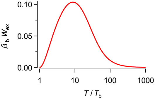
Figure 3. Extractable work is a non-monotonic function of initial temperature T = β⁻¹ for the double-well potential of Figure 1A.

In addition to having a clear physical interpretation, W_ex(β, β_b) is easily calculated as a simple numerical integral of equilibrium Gibbs-Boltzmann distributions for two temperatures. By contrast, to establish the non-monotonicity of a₂, the criterion of Lu and Raz [1], one must first find the left eigenfunction u₂ by solving the boundary-value problem associated with the adjoint Fokker-Planck operator.

5. Discussion

The anomalous relaxation process known as the Mpemba effect is defined by a non-monotonic dependence of relaxation time on initial temperature. Lu and Raz [1] showed that an equivalent criterion is the non-monotonicity of the a₂ projection coefficient derived from an associated Fokker-Planck equation. In this Brief Research Report, we have shown that, for a 1D potential U(x) with a metastable and a stable minimum, the Mpemba effect can be viewed as a simple two-stage relaxation in the function space of all admissible probability densities. In the fast Stage 1, the system relaxes to a local equilibrium. In the slow Stage 2, the populations in the two coarse-grained states equilibrate. In such a situation, we have shown that the Mpemba effect is associated with a non-monotonic temperature dependence of the maximum extractable work of the local equilibrium stage reached at the end of Stage 1. Relative to the a₂ coefficient, extractable work is a much more physical quantity that is also much easier to calculate.

The physical picture offered here, for a double-well potential, meets our goal: We can relate the existence of the Mpemba effect to a non-monotonicity of the extractable work. However, we have not carefully characterized the range of validity of the approximations used in our analysis. For example, in writing Equation (9), we assume that the fraction of initial systems that start in either state (x < 0 or x > 0) is preserved after the initial fast transient. In fact, even during the brief transient, calculating the fraction of systems in each region is subtle, a point emphasized by van Kampen [32] in a careful study that would be the starting point for a more detailed theoretical investigation.

Although our arguments assume a 1D potential with two local states, they generalize easily to many dimensions and many local states. In such cases, the state vector has a large number of dimensions, and solving the Fokker-Planck equation or even calculating its eigenfunctions is difficult. But calculating the extractable work remains easy. Of course, our arguments do not imply that the Mpemba effect can occur only in potentials with metastable states and leave open the possibility for other scenarios.

Data Availability Statement

The original contributions presented in the study are included in the article/Supplementary Material, further inquiries can be directed to the corresponding author/s.

Author Contributions

RC conceived the project and originated the overall theory. AK carried out calculations using parameters based on his previous experimental results and prepared figures. JB oversaw the project and contributed to the theory and discussion. All authors participated in writing and editing the paper.

Funding

JB and AK were supported by NSERC Discovery and RTI Grants (Canada). RC acknowledges support from the Pacific Institute for Mathematical Sciences (PIMS), the French Centre National de la Recherche Scientifique (CNRS) that made possible his visit to Vancouver and the project RETENU ANR-20-CE40-0005-01 of the French National Research Agency (ANR).

Conflict of Interest

The authors declare that the research was conducted in the absence of any commercial or financial relationships that could be construed as a potential conflict of interest.

Supplementary Material

The Supplementary Material for this article can be found online at: https://www.frontiersin.org/articles/10.3389/fphy.2021.654271/full#supplementary-material

Footnotes

References

Appendix

1. Monotonicity of Kullback-Leibler divergence along G_leq. The Kullback-Leibler divergence [33] can be written in terms of Equation (9) as

In the second line, we omit the corresponding a_R terms. In the third line, $a_{\text{L}}^{*}\equiv {\int }_{-\infty }^0\text{d}x{g}_{{\beta }_{\text{b}}}(x)$ and $a_{\text{R}}^{*}\equiv {\int }_0^{\infty }\text{d}x{g}_{{\beta }_{\text{b}}}(x)$. In the fourth line, the vectors represent two-state probability distributions. Note that in the “short Stage 1” approximation of Equation (10), the final expression for D_KL involves two coarse-grained probability distributions, with $\begin{array}{l}\left(\begin{array}{l}{a}_{\text{L}}\hfill \\ a_{\text{R}}\hfill \end{array}\right)\end{array}$ depending only on β and $\begin{array}{l}\left(\begin{array}{l}{a}_{\text{L}}^{*}\hfill \\ a_{\text{R}}^{*}\hfill \end{array}\right)\end{array}$ only on β_b.

We then investigate the monotonicity of D_KL $\left[\left(\begin{array}{l}{a}_{\text{L}}\hfill \\ a_{\text{R}}\hfill \end{array}\right),\left(\begin{array}{l}{a}_{\text{L}}^{*}\hfill \\ a_{\text{R}}^{*}\hfill \end{array}\right)\right]$ by differentiating:

which is positive for $a_{\text{L}}>a_{\text{L}}^{*}$ and negative for $a_{\text{L}}<a_{\text{L}}^{*}$. (Recall that $a_{\text{L}}+a_{\text{R}}=a_{\text{L}}^{*}+a_{\text{R}}^{*}=1$.) Thus, $D_{\text{KL}}\left({\rho }^{\text{leq}},g\right)$ is monotonic in a_L on either side of equilibrium.

2. Proof of Equation (15). The relationship is well known [34] and holds for any distribution, including ones describing local equilibrium. Below, to simplify notation, we write ρ^leq for ${\rho }_{\beta ,{\beta }_{\text{b}}}^{\text{leq}}$ and g for g_βb.

which is equivalent to Equation (15).

References

1. Lu Z, Raz O. Nonequilibrium thermodynamics of the Markovian Mpemba effect and its inverse. Proc Natl Acad Sci USA. (2017) 114:5083–8. doi: 10.1073/pnas.1701264114
2. Amir A, Oreg Y, Imry Y. On relaxations and aging of various glasses. Proc Natl Acad Sci USA. (2012) 109:1850–5. doi: 10.1073/pnas.1120147109
6. Chaddah P, Dash S, Kumar K, Banerjee A. Overtaking while approaching equilibrium. arXiv:10113598. (2010).
7. Ahn YH, Kang H, Koh DY, Lee H. Experimental verifications of Mpemba-like behaviors of clathrate hydrates. Korean J Chem Eng. (2016) 33:1903–7. doi: 10.1007/s11814-016-0029-2
8. Lorenzo AT, Arnal ML, Sanchez JJ, Müller AJ. Effect of annealing time on the self-nucleation behavior of semicrystalline polymers. J Polym Sci Part B: Polym Phys. (2006) 44:1738–50. doi: 10.1002/polb.20832
9. Hu C, Li J, Huang S, Li H, Luo C, Chen J, et al. Conformation directed Mpemba effect on polylactide crystallization. Cryst Growth Des. (2018) 18:5757–62. doi: 10.1021/acs.cgd.8b01250
10. Greaney PA, Lani G, Cicero G, Grossman JC. Mpemba-like behavior in carbon nanotube resonators. Metall Mater Trans A. (2011) 42:3907–12. doi: 10.1007/s11661-011-0843-4
11. Lasanta A, Reyes FV, Prados A, Santos A. When the hotter cools more quickly: Mpemba effect in granular fluids. Phys Rev Lett. (2017) 119:148001. doi: 10.1103/PhysRevLett.119.148001
12. Baity-Jesi M, Calore E, Cruz A, Fernandez LA, Gil-Narvión JM, Gordillo-Guerrero A, et al. The Mpemba effect in spin glasses is a persistent memory effect. Proc Natl Acad Sci USA. (2019) 116:15350–5. doi: 10.1073/pnas.1819803116
14. Vynnycky M, Mitchell S. Evaporative cooling and the Mpemba effect. Heat Mass Transfer. (2010) 46:881–90. doi: 10.1007/s00231-010-0637-z
15. Mirabedin SM, Farhadi F. Numerical investigation of solidification of single droplets with and without evaporation mechanism. Int J Refrig. (2017) 73:219–25. doi: 10.1016/j.ijrefrig.2016.09.006
16. Vynnycky M, Kimura S. Can natural convection alone explain the Mpemba effect? Int J Heat Mass Transfer. (2015) 80:243–55. doi: 10.1016/j.ijheatmasstransfer.2014.09.015
17. Auerbach D. Supercooling and the Mpemba effect: when hot water freezes quicker than cold. Am J Phys. (1995) 63:882–5. doi: 10.1119/1.18059
18. Wojciechowski B, Owczarek I, Bednarz G. Freezing of aqueous solutions containing gases. Cryst Res Technol. (1988) 23:843–8. doi: 10.1002/crat.2170230702
19. Zhang X, Huang Y, Ma Z, Zhou Y, Zhou J, Zheng W, et al. Hydrogen-bond memory and water-skin supersolidity resolving the Mpemba paradox. Phys Chem Chem Phys. (2014) 16:22995–3002. doi: 10.1039/C4CP03669G
20. Risken H. The Fokker-Planck Equation: Methods of Solution and Applications. 2nd Edn. Berlin: Springer (1989). doi: 10.1007/978-3-642-61544-3
21. van Kampen NG. Stochastic Processes in Physics and Chemistry. 3rd Edn. Amsterdam: Elsevier (2007). doi: 10.1016/B978-044452965-7/50006-4
22. Hänggi P, Thomas H. Stochastic processes: time evolution, symmetries and linear response. Phys Rep. (1982) 88:207–319. doi: 10.1016/0370-1573(82)90045-X
23. Gardiner CW. Stochastic Methods: A Handbook for the Natural and Social Sciences. 4th Edn. Berlin: Springer (2009).
24. Seifert U. Stochastic thermodynamics, fluctuation theorems and molecular machines. Rep Prog Phys. (2012) 75:126001. doi: 10.1088/0034-4885/75/12/126001
25. Kumar A, Bechhoefer J. Exponentially faster cooling in a colloidal system. Nature. (2020) 584:64–8. doi: 10.1038/s41586-020-2560-x
26. Klich I, Raz O, Hirschberg O, Vucelja M. Mpemba index and anomalous relaxation. Phys Rev X. (2019) 9:021060. doi: 10.1103/PhysRevX.9.021060
27. Kramers HA. Brownian motion in a field of force and the diffusion model of chemical reactions. Phys A. (1940) 7:284–304. doi: 10.1016/S0031-8914(40)90098-2
28. Hänggi P. Reaction-rate theory: fifty years after Kramers. Rev Mod Phys. (1990) 62:251–341. doi: 10.1103/RevModPhys.62.251
29. Berglund N. Kramers' law: validity, derivations and generalisations. Markov Process Relat Fields. (2013) 19:459–90.
30. Gavrilov M, Chétrite R, Bechhoefer J. Direct measurement of nonequilibrium system entropy is consistent with Gibbs-Shannon form. Proc Natl Acad Sci USA. (2017) 114:11097–102. doi: 10.1073/pnas.1708689114
31. Parrondo JMR, Horowitz JM, Sagawa T. Thermodynamics of information. Nat Phys. (2015) 11:131–9. doi: 10.1038/nphys3230
32. van Kampen NG. A soluble model for diffusion in a bistable potential. J Stat Phys. (1977) 17:71–87. doi: 10.1007/BF01268919
33. Cover T, Thomas J. Elements of Information Theory. 2nd Edn. New York, NY: John Wiley & Sons, Inc. (2006).