Implementation of a Compact Spot-Scanning Proton Therapy System in a GPU Monte Carlo Code to Support Clinical Routine

1. Introduction

In radiation therapy, the treatment planning system (TPS) is a crucial part of the clinical workflow. Based on anatomical information about the patient, typically derived from X-ray computed tomography (CT) images, this software predicts the dose administered to a patient in a given irradiation scenario and inversely optimizes the treatment plan starting from a desired dose distribution. The dose engine in a TPS needs a sufficiently precise model of the treatment machine to be able to make accurate dose estimates. This is particularly true for proton therapy because the protons’ dose distribution includes sharp spatial gradients which can lead to severe under- or overdosage if incorrectly delivered. Dose recalculation based on an independent dose engine can be an important element of quality assurance (QA) [1, 2]. The expected benefit is to achieve better overall QA and to reduce machine time for QA measurements. This contribution describes the implementation of our proton treatment system in a fast MC software to eventually build such a QA tool.

Traditionally, dose engines in proton therapy have relied on numerical algorithms which use analytical models of the proton beam and its propagation through the patient. Often, these algorithms need to make some simplifying assumptions about the detailed interaction of protons with the complex tissue distribution inside the patient. More recently, Monte Carlo (MC) codes have become an alternative tool for dose calculation. Such codes transport particles one by one across objects of interest and evaluate physical interactions step-by-step along each particle’s trajectory. MC simulations offer more accurate modeling of proton interactions with heterogeneous media and improved dose calculation accuracy in complex geometries with respect to analytical pencil beam algorithms [3, 4].

General purpose MC simulation toolkits originally developed in other fields of physics including accelerator and particle physics have been used in the context of proton therapy. These include FLUKA [5–7], Shield-HIT [8], and Geant4 [9], as well as Geant4-based applications specific to medical physics like GATE/GATE-RTion [10, 11] and TOPAS [12, 13]. However, a challenging factor when attempting to employ MC simulation in daily clinical routine is the long calculation time (on the order of hours on multiple CPUs) [3]. To address this, GPU-accelerated MC codes started to be investigated in the field of proton therapy, for example, gPMC, Fred, and a code developed at the Mayo Clinic [14–17]. GPU acceleration has also been exploited to speed up analytical dose engines [18], yet without the precise physics modeling of MC. We decided to use the GPU-accelerated MC code Fred [16] in our proton facility, the Maastro proton therapy center in Maastricht (Netherlands).

Before a MC code can be used for recalculating patient plans, the simulation needs to be implemented in such a way as to mimic the clinical proton beam irradiating the patient. This step is essential to guarantee accurate dose prediction. Previous authors have presented the MC implementations of their treatment machines, and approaches can be roughly sorted into two categories. On the one hand, the treatment machine is purely described by an effective phase space which is conveniently parameterized [19, 20]. In other words, the MC simulation has no explicit knowledge about the proton beam line, and particles are generated at the exit nozzle directly according to the phase space parameterization and tracked from that point on. On the other hand, a full geometrical description of the proton beam line or at least the exit nozzle can be implemented in the Monte Carlo simulation so that particles are explicitly transported through these parts of the beam line [21–23]. This latter approach is not optimal from the point of view of computation speed as protons need to be tracked over again through the same beam line for each new patient.

The peculiarities of the treatment system in our facility, a Mevion S250i Hyperscan system, were such that none of the existing methods in the literature were directly applicable. Rather, we needed to design a new hybrid method to implement our treatment machine in Fred. Specifically, the Mevion system uses one fixed pristine beam energy which is reduced by degrader plates in the nozzle. The nozzle is positioned in air downstream of the beam’s vacuum pipe. Furthermore, the collimator leaves of an adaptive aperture continuously move into and out of the beam during a patient irradiation. Finally, the entire beam nozzle is extendable, and its distance to the isocenter may vary during treatment. Existing methods where the proton beam is described by an effective phase space model would not have been feasible because one parameterization of such a model would have been necessary for each possible configuration of the nozzle. We therefore chose an approach where the proton beam is described via a phase space model upstream of the nozzle and then tracked explicitly across the nozzle. A practical concern was that the nozzle can move so close to the patient that in the simulation it would overlap with the box containing the voxelized patient CT image. We implemented a dedicated new functionality in Fred to cope with this. Finally, the continuously changing nozzle geometry required optimized geometry handling in Fred to efficiently communicate with the GPU hardware.

In this work, we present the implementation of our treatment machine in Fred, the optimization of model parameters based on experimental data acquired during the commissioning of the facility [24], and validation based on additional data. Finally, we compare dose distributions recalculated with Fred and with the clinical TPS.

2. Materials and Methods

2.1. The Mevion S250i

The Mevion S250i Hyperscan system (cf. Figure 1) is a small superconducting synchrocyclotron with only 15 tons and a diameter of 1.8 m. It consists of two coaxial gantries. The superconducting synchrocyclotron (10 T) with the ion source and the scanning magnets is mounted on the outer gantry. The inner gantry carries the beam monitor system, the range modulation system, and a multi-leaf collimator system referred to as “adaptive aperture”. The components taken into account in Fred, that is, the range shifter, the adaptive aperture, and the nozzle window, are sketched in Figure 2. For more details, we also refer to [24].

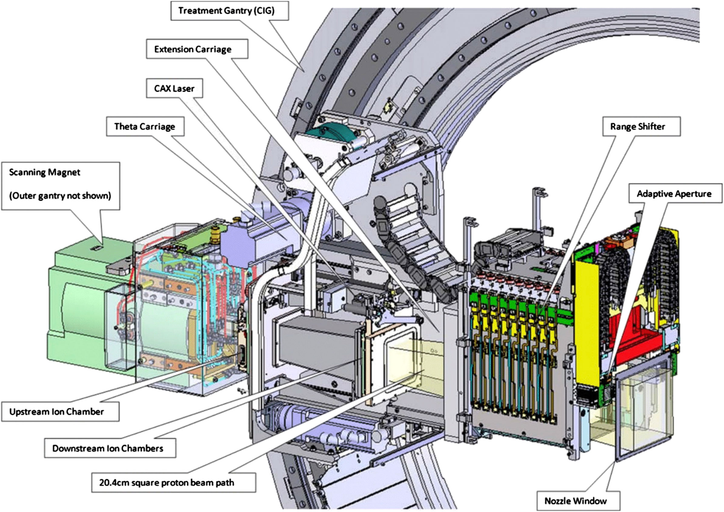
FIGURE 1. Layout of the Mevion S250i. Courtesy of Mevion.

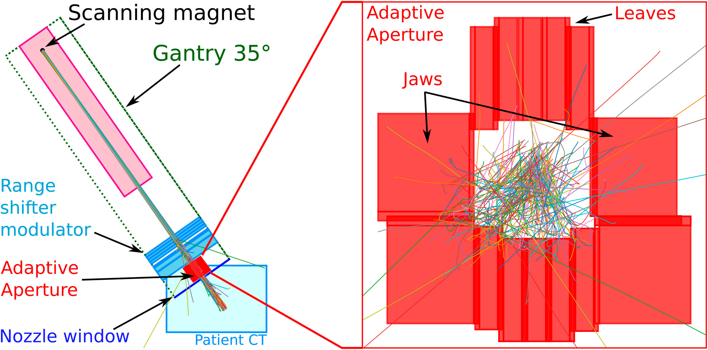
FIGURE 2. Elements of the beam model.

The system accelerates a fixed energy beam of about 230 MeV, the so-called pristine energy, and extracts it toward the single treatment room. The treatment line is equipped with a dose delivery system and an extendable nozzle at the end of the beam line. The dose delivery system consists of three elements: a thin 80 quadrant foil position detector, the beam scanning magnet, and six transmission ionization chambers or beam monitors. The vacuum window is located immediately after the scanning magnets, at about 2 m from the room isocenter, and all components mounted on the inner gantry are in air. To obtain clinically relevant energies, which cover a range from 0 cm to 32.2 cm in water, the pristine energy is degraded by the range modulation system, mounted in the nozzle. It consists of 18 Lexan plates of different thicknesses whose combinations allow the generation of 161 energies with 2.1 mm range steps in water. The distance from the nozzle window to the isocenter is adjustable from 3.6 to 33.6 cm. The adaptive aperture is the most downstream functional element of the beam line, also mounted in the nozzle. The gantry system can rotate from 355° to 185° with an angular accuracy of ±0.25°. The 360° beam entrance coverage is achieved by rotating the six-degrees-of-freedom robotic couch.

The Maastro proton therapy center started clinical activity in February 2019, and 137 patients have been treated since then. The clinical TPS at the time of writing this study is RayStation version 9B (RaySearch Laboratories, Sweden) which uses a Monte Carlo dose engine (on CPU).

2.2. Implementation of Proton Beam Source in Fred

To implement the therapeutic proton beam source of the Mevion accelerator system in Fred, we used a phase space model to describe the pristine proton beam in a plane downstream of the scanning magnets and simulated explicitly in Fred the geometry of the components included in the extendable nozzle, that is, the range shifter, the adaptive aperture, and the nozzle window. We will use the term “beam model” to refer to a combination of both.

In particular, the phase space model was split into a longitudinal component (energy spectrum) and a transverse component (beam shape), both modeled empirically as Gaussian distributions. This kind of phase space description had already been used successfully by other authors [19]. The longitudinal phase space component is parameterized by the mean proton energy and the energy spread (variance) and the transverse component by the width of the transverse distribution (beam size, i.e., variance).

The beam size evolves along the beam axis as a function of distance z from the virtual source plane $\left(z=0\right)$. The propagation beam model used in this work is the so-called emittance model, that is, the beam evolution in phase space is characterized by a constant emittance, both in x and y directions. Equation 1 describes the evolution of the envelope of the beam in one transverse direction along the propagation direction z. The model has three parameters per transverse direction [25] and describes what is called a drift in accelerator language, namely, a section of the beam line where no active elements (such as bending magnets or focusing quadrupoles) are present. We are considering the beam section after the focusing optics (quadrupole magnets) so that the waist of the beam, that is, the position where the beam width is minimal, is downstream of the source plane (as it can be seen in Figure 3). The emittance model is used when the virtual point source model is not accurate enough, namely, when the focal length of the last quadrupoles is relatively short. The Mevion machine is in fact a compact accelerator, with a Rayleigh length of about 1 m.

Clearly, the emittance model is only valid if ${\sigma }^2>0$ for all z. Furthermore, because the quadrupole magnets of the proton beam line focus the beam, one has $\partial {\sigma }^2/\partial z<0$ from the magnets down to the beam waist. Regarding the model parameters, the emittance ϵ determines the area of the beam distribution in the phase space and must be positive, β is the characteristic length over which the beam size changes and must be positive, and α determines whether the beam is focusing $\left(\alpha >0\right)$ or defocusing $\left(\alpha <0\right)$.

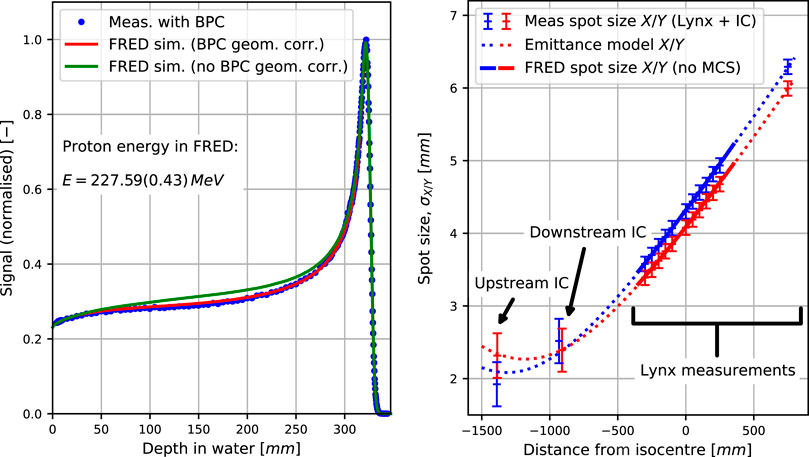
FIGURE 3. (Left) Bragg peaks measured with the Bragg peak chamber (BPC) of diameter 81.6 mm and simulated for the optimal energy and energy spread in the BPC, mimicking the experimental setup, as well as in full 40 × 40 × 40 cm³ water phantom for comparison. (Right) Emittance model fit to measured spot sizes (Lynx and IC) in the in-plane (X) and cross-plane (Y) directions along with the beam sizes simulated with Fred in air without multiple Coulomb scattering.

It is important to underline that the source plane (where z = 0) only plays the role of a reference frame in which the protons are generated. The beam size is purely determined by the three parameters α, β, and ε. This is different from a virtual point source model where the point source position determines the beam divergence.

The clinical TPS uses the so-called monitoring units (MU) as a dosimetric scale based on an internal calibration. The Monte Carlo code, on the other hand, requires the number of primary protons to be specified. Therefore, a scaling factor is needed to parameterize the relationship between the two quantities (cf. Section 2.4.3).

The explicitly implemented nozzle components are the adaptive aperture, the range modulation system, and the nozzle window. Their size, placement, and composition were taken from the manufacturer’s specifications of the proton accelerator. The aperture leaves have a step-like interleaving structure to reduce proton leakage when closed. This was constructed in Fred as a composition of 60 cuboid regions. The elemental composition of the energy degrader plates was fixed, but their mass density was optimized as a part of the beam model calibration (cf. Section 2.4.4).

2.3. New Functionality in Fred

Two new technical features needed to be implemented in Fred. The first one was due to the fact that the beam nozzle of the Mevion system is extendable. In some treatment configurations, this leads to an overlap in the simulation of the cuboid regions enclosing the beam nozzle and patient geometry. In which of the two regions, a proton needs to be tracked then becomes ambiguous. To cope with this specific problem, Fred now allows specifying the region where a proton was generated, that is, the nozzle region, propagates protons up to the boundaries of this region, and only then switches to the overlapping patient volume.

The second issue was the variability of the nozzle’s geometrical configuration. More specifically, each beam spot delivered to the patient potentially has a different set of degrader plates moved into the beam path as well as a different positioning of the adaptive aperture. The initial approach to implement this was to iteratively communicate the current configuration of the simulated geometry to the GPU and track the protons belonging to the associated beam spot. This led to an interfering computational overhead which prevented the GPU from exploiting its potential. Most of the simulation was actually spent in handling the communication with GPU. A new scheme was therefore implemented in which all configurations of the geometry are communicated once to the GPU at the beginning. Each simulated pencil beam is internally associated to a specific configuration in which it needs to be tracked. In this way, all protons in a treatment plan can be tracked on the GPU without interruption.

2.4. Beam Model Calibration

The beam model was calibrated according to the following overall scheme: experimental data were acquired as a part of the facility commissioning or specifically for this work. Details about the commissioning can be found in [24]. The measurement conditions were mimicked in Fred, and the beam model parameters were determined by optimizing the match between measured and simulated data. The following sections describe the calibration in detail.

2.4.1. Transverse Phase Space Component—Emittance Model

The emittance model describes the beam spot size in air as a function of the position along the beam axis (cf. Equation 1). To calibrate the model parameters, transverse profiles of the pristine beam were measured at twelve distances from the isocenter using a scintillator detector (IBA Lynx, Louvain-la-Neuve, Belgium). The nozzle window was removed during the measurements because it would alter the pristine beam. To avoid confusion, we recall that the nozzle window is not the end of the vacuum beam line, but only a protective cover of the air-filled nozzle.

The spot size at each measured distance was determined as standard deviation, σ, of a Gaussian fit to the cross-plane and in-plane profiles through the spot mass center. Additionally, the spot sizes measured by the beam monitor system in the nozzle were used. The emittance model parameters were determined by fitting Equation 1 to the set of spot sizes, as a function of depth. No constraints were imposed on the parameters in the fit routine, but the plausibility of the fit parameters was checked manually.

2.4.2. Longitudinal Phase Space Component—Pristine Energy

The laterally integrated depth dose distribution (IDD) of the pristine energy was measured with a large-area plane-parallel ionization chamber of 8.16 cm diameter (Bragg Peak IC TM34070, PTW, Freiburg, Germany) mounted on the mechanical arm of a water phantom (PTW MP3-PL). The nozzle window was removed during the measurements (cf. Section 2.4.1). The distance from the virtual source plane (scanning magnets position) to the isocenter was fixed to 182.14 cm for all gantry angles and the same for the cross-plane and in-plane scanning directions.

Fred simulations were performed in a 40 × 40 × 40 cm³ virtual phantom of 1 × 1 × 1 mm³ voxel size, mimicking the measurement setup. The ionization potential of water was set to 78 eV. The geometrical acceptance due to the limited size of the Bragg Peak IC was taken into account in Fred.

Simulated and measured IDDs were analyzed by fitting an analytical model [26], as well as by using a spline function. The beam model parameters, that is, beam energy and energy spread, were found by matching the measured and simulated IDDs, minimizing differences of full width at half maximum (FWHM) and the range, defined as 80% of the maximal value at the distal falloff.

2.4.3. Dosimetric Calibration Factor

The scaling factor was determined based on absolute dose measurements of a uniform 10 × 10 cm² monoenergetic field with 1,000 MU for the whole plan consisting of 1,681 spots. Dose was measured at a depth corresponding to 1/4 of the proton range in water, which was 79 mm, with a plane-parallel ionization chamber (IBA PPC05) positioned in a water tank (PTW MP3-PL). The size of the active volume of the PPC05 detector (diameter of 9.9 mm and thickness of 0.6 mm) was considered in the analysis of the Fred simulations to estimate the mean dose in this volume. The scaling factor was determined by matching simulated and measured dose.

2.4.4. Range Modulation System

The thickness and position of the Lexan plates in the range modulator system were extracted from the manufacturer’s technical drawings. The density of each modulation plate was optimized in Fred, following the procedure of the clinical TPS. In particular, for each range modulator plate, depth dose profiles in water were measured and simulated with and without the plate present. The range was determined as the depth in water at 80% of the maximum value at the distal Bragg peak falloff. Each plate’s water equivalent thickness was determined as the difference in range with and without plate.

2.4.5. Adaptive Aperture

The adaptive aperture module consists of two carriages of five leaves, each 5 mm wide (in-plane direction, i.e., perpendicular to the leaves’ movement), and one top and one bottom jaw, each 20 mm wide, made of nickel alloy (cf. Figure 2). The thickness of the leaves and jaws in the beam direction is 100 mm. The aperture can trim spots laterally over a 20 × 20 cm² area at the isocenter plane. The inner surface of the leaves has an interlocking tongue and groove shape to prevent leakage when the collimators are closed. This was implemented in Fred based on technical drawings using 60 cuboid regions, that is, the cuboid regions were combined in such a way as to approximately represent the shape of the aperture leaves.

Commissioning of the beam delivery system includes a procedure to adjust the alignment of the adaptive aperture in the in-plane and cross-plane directions with respect to the beam axis. This was reproduced in Fred as part of the beam model calibration. To this end, the snout position was set to 19.5 cm, and five range modulator plates were inserted to broaden the beam. The aperture was closed, except for the middle leaves which were opened ±2.5 cm, leaving a square-shaped opening of about 5 × 5 mm². A 3 × 3 cm² field was irradiated in a regular spot grid of 2.5 mm steps. The dose was scored in a water phantom positioned at the isocenter at 5 mm below the water surface.

Moving the adaptive aperture in in-plane and cross-plane directions, an offset with respect to its nominal position (from the technical drawings) was determined in Fred to obtain symmetrical transverse dose profiles.

2.5. Beam Model Validation

2.5.1. Pencil Beams in Water

The range shifter model was validated with measurements performed during commissioning of the facility. In particular, laterally integrated depth dose profiles were measured with an ionization chamber (Bragg Peak IC TM34070 from PTW) in a water phantom at selected clinically available energy settings. Transverse profiles of single spots were measured in water with a microdiamond detector (PTW TN60019). The nozzle window was present during the measurements.

It is important to point out the difference between the calibration and validation measurements. Both were performed with the same kind of equipment and following the same measurement principle. The difference lies in the combination of degrader plates in either case. For the calibration measurements, individual plates were inserted into the beam so that the retrieved calibration parameters corresponded to this plate specifically. The independent validation measurements used clinical energy settings which generally require combinations of multiple degrader plates to be inserted into the beam. In this sense, the validation measurements were used to assess the consistency of the calibration parameters.

2.5.2. Monoenergetic Layers in Water

Dose coverage in a proton therapy treatment is achieved by overlapping multiple pencil beams with different transverse positions. It is therefore important to verify that the total dose in such a scenario is correctly simulated in Fred. To this end, absolute point dose was measured in the water phantom for single energy layers at different field sizes. We used the PPC05 (IBA) for fields larger than 5 × 5 cm², a semi-flex 3D ionization chamber (PTW TN31021) for 5 × 5 cm² and 4 × 4 cm² fields, and a microdiamond detector (PTW TN60019) for the 3 × 3 cm² field. Absolute point dose was measured for 15 energies and nine field sizes (i.e., overall 135 measurements) at the depth of 1/4 of the BP position in water. The isocenter was located at 19.9 mm depth in water, and the snout position was 30.01 cm, that is, the air gap to the water surface was 10.11 cm. The nozzle window was present during the measurements. The dose layers were simulated in Fred, and absolute point dose measurements were compared. The size of the detector was taken into account when analyzing Fred dose simulations by calculating the mean dose in the detector volume. No adaptive aperture was used for the measurements.

2.5.3. Dose Cubes in Water

A 3D proton dose volume is achieved by combining multiple energy layers, that is, pencil beams of different energies which form a spread-out Bragg peak (SOBP). Their relative weights are optimized to best match the required dose distribution.

Following common protocols in proton therapy, we used cube-shaped dose distributions to validate the simulation accuracy of Fred. In particular, absolute point dose of spread-out Bragg peaks in water was measured with an ionization chamber along the central axis and off-axis, at three depths each, of a 125 cm³ cube at 5 and 10 cm depth and of a 1,000 cm³ cube at 10 cm depth. In sum, six measurement points per cube were measured. The prescribed dose level was 1.82 Gy (2 Gy (RBE)). The dose cubes were simulated in Fred and compared with the absolute point dose measurements. The size of the ionization chamber was taken into account when analyzing Fred dose simulations. All plans included the adaptive aperture.

2.5.4. Patient Quality Assurance

A useful application of Fred in clinical practice would be to reproduce patient QA measurements via simulation. This could help to reduce the amount of manual QA tasks in clinical routine. In our proton facility, patient QA measurements are performed with an array of ionization chambers (OCTAVIUS 1500 XDR) in RW3 solid water measuring 2D dose distributions at a few selected depths. We implemented the experimental procedure also in Fred and compared the results against the experimental data. The depth in the RW3 solid water phantom used for the measurements was recalculated into water equivalent depth by rescaling with the RW3’s relative stopping power by 1.045. We tested Fred for all clinical patient plans delivered in our proton facility since clinical operation began in 2019, that is, around 300 QA plans for different indications (i.e., head and neck (8%), brain (18%), breast (29%), lung (36%), lymphoma (3%), and esophagus (6%) tumors). The simulations were performed with 10⁵ protons/spot in a 1 mm³ dose grid in a virtual water phantom.

The gamma index analysis was applied to compare 2D dose slices extracted from simulated 3D dose distributions to 2D measured dose distributions. As criteria, we used a dose difference (DD) of 2% or 3% (local dose), distance to agreement (DTA) of 2 mm or 3 mm, and a dose cutoff (DCO) of 2%, in accordance with clinical protocols.

2.6. Full Simulations of Patient Plans

Another clinical application of Fred is to recalculate the full treatment plans in the patient geometry provided by CT images. The photon attenuation coefficients in a CT image must be converted into quantities required by Fred, that is, mass density, relative stopping power, elemental composition, and radiation length. We implemented the two-step conversion method presented in [27], which uses a conversion from photon attenuation to mass density and one from mass density to the other quantity. The former can be obtained from phantom-based CT calibration and was readily available in our facility. The latter is based on a set of tissue descriptions representative of the human body and piecewise linear interpolations of the quantities of interest. We used the same tissues as in [27] and extended the parameters provided therein with radiation length values for each tissue (http://pdg.lbl.gov/2020/AtomicNuclearProperties/). This calibration procedure is similar to the one in RayStation, although we had now access to the implementation details.

To test the beam model, we recalculated several patient plans including the brain, head and neck, breast, and lung cases (5 each). Simulations were run with 10⁵ protons per spot.

3. Results

3.1. Beam Model Calibration

3.1.1. Transverse Phase Space Component

The right panel of Figure 3 reports the beam spot size in air as a function of distance from the isocenter. Data points were measured inside the nozzle by built-in beam monitors as well as outside of the nozzle as explained in Section 2.4.1. The dotted lines represent the emittance model fitted to the data, and the solid lines were obtained in the Fred simulation in air using the model, that is, reproducing the measurement. The simulated spot sizes in the treatment area, that is, ±35 cm around the isocenter, agree with the measurements better than 0.03 mm, showing that the fit results are consistent. According to the fitted emittance model, the beam waist (i.e., its narrowest point) lies between −1,000 mm and −1,300 mm. This is reasonable because the quadrupole magnets first focus the beam before it subsequently diverges toward the isocenter (cf. Section 2.2).

3.1.2. Longitudinal Phase Space Component

The left panel of Figure 3 compares simulated and measured integrated depth dose profiles in water of a pristine proton beam, that is, without range modulator plates and the nozzle window. This configuration has no corresponding nominal energy as nominal energies are only defined with the nozzle window mounted. When accounting for the geometrical acceptance of the Bragg peak chamber (red curve), the simulated profile matches very well with the measurements, achieving BP range and FWHM differences below 0.05 mm.

The two parameters of the longitudinal phase space component of the proton source model, that is, the mean initial energy and the Gaussian energy spread, were determined by matching simulated and measured data (cf. Section 2.4.2). They were thus determined to be 227.59 MeV and 0.43 MeV, respectively.

3.1.3. Dosimetric Calibration Factor

The scaling factor from monitoring units to the number of primaries was calculated to be 7.417 ×10⁷ protons/MU.

3.1.4. Range Modulation System

Figure 4 shows integrated depth dose profiles in water with a few selected individual range modulator plates or the nozzle window inserted into the beam path. The measured profiles (dots) match the simulated ones (solid) well. The legend reports the water equivalent thickness of the plates determined from measured and simulated data, respectively. Agreement for all the range modulator plates and the nozzle window was better than 0.1 mm. It is worth noting that a good match is obviously expected because the simulated degrader plate densities were calibrated to achieve this (cf. Section 2.4.4). In this sense, the residual mismatch of 0.1 mm is indicative of the goodness of the calibration procedure and not of the range accuracy in dose calculation which was instead verified by the calibration.

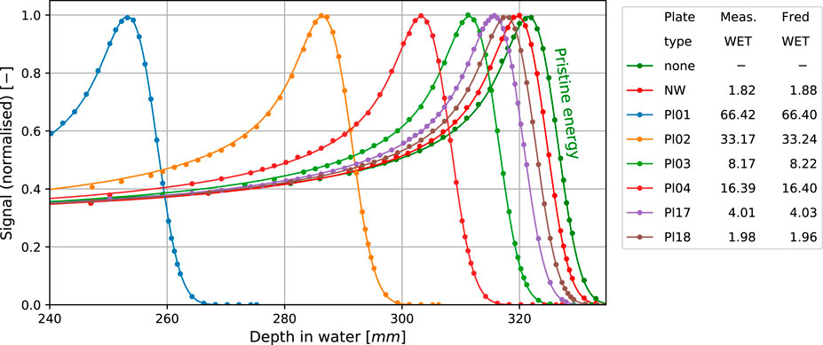
FIGURE 4. Measured (dots) and simulated (solid lines) BPs for selected RS plates and the nozzle window (NW) WET compared to the BP of pristine energy. All the simulation results account for the geometrical acceptance correction for the BPC. The table presents calculated and measured WET in mm.

3.1.5. Adaptive Aperture

The adaptive aperture implemented in Fred was aligned with the beam axis as described in Section 2.4.5. The offset to be applied in Fred with respect to the nominal aperture position (from technical drawings) was found to be 0.995 mm in the in-plane direction, that is, perpendicular to the leaves, movement, and −0.005 mm in the cross-plane direction, that is, along the leaves’ movement.

3.2. Beam Model Validation

3.2.1. Pencil Beams in Water

Figure 5 presents validation results for single pencil beams in water for selected beam energies (range shifter plate configurations) as explained in Section 2.5.1. Blue dots and red lines show measured and simulated integrated depth dose profiles, respectively. Measured and simulated data match very well in the plateau region and around the Bragg peak, indicating Fred accurately reproduces electromagnetic energy loss and pileup due to nuclear interactions. The agreement between measured and simulated range is better than 0.25 mm for all combinations of range modulator plates.

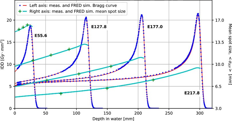
FIGURE 5. Comparison of simulated (solid lines) and measured BPs (dots) and spot sizes (crosses) in water for four main nominal energies (in MeV): E55.6, E127.8, E177.0, and E217.8. All the simulated Bragg curves account for the geometrical acceptance of the Bragg peak chamber detector.

The green data points and light blue curves (referring to the right ordinate) show the measured and simulated beam spot size at different depths in water. Agreement is better than 0.5 mm for all data points and thus well within clinical acceptance criteria.

3.2.2. Monoenergetic Layers in Water

We used monoenergetic layers in water to validate the dosimetric accuracy of Fred when multiple pencil beams are superimposed, as explained in Section 2.5.2. The left and center panels of Figure 6 show the relative difference of the measured and simulated dose, that is, in Fred and TPS. The average relative differences between measurement and Fred do not exceed ±2%, except for very small fields of 1 × 1 cm² and 2 × 2 cm². It should be noted that uncertainty in the detector position is particularly important in small fields and likely to be (partially) responsible for the these larger differences. In any case, Fred is at least as accurate as the clinical TPS. The right panel depicts the mean proton range difference between Fred and TPS determined from the distal falloff of the dose cube’s central axis profiles. The slight systematic discrepancy remains within −0.3 mm and 0.1 mm and is clinically acceptable.

FIGURE 6. Relative differences between measured doses calculated in Fred and the TPS as a function of nominal energy (left panel) and field size (center panel), as well as absolute range differences between Fred and the TPS as a function of nominal energy (right panel). Each data point represents the average over all field sizes in the left and right panels and over all energies in the center panel. The error bars indicate minimum and maximum values in a group.

3.2.3. Dose Cubes in Water

Dosimetric validation based on dose cubes in water was performed to quantify the accuracy of Fred dose simulations when multiple pencil beams of various energies are superimposed in the transverse and longitudinal direction. Simulations were run with 10⁶ protons per spot on a single GPU and took 2 min for the 125 cm³ cube and 7 min for the 1,000 cm³ cubes. Figure 7 shows example profiles across two dose cubes simulated with the TPS and Fred and measured, as explained in Section 2.5.3. Relative dose differences with Fred and the TPS are of similar magnitude. The relative dose difference between simulation and measurement averaged over the six data points per cube were

• $+{0.19}_{-0.17}^{+0.90}\left(0.37\right)\text{\%}$ for the 125 cm³ cube placed at 5 cm depth,

• $-{1.00}_{-1.55}^{-0.27}\left(0.51\right)\text{\%}$ for the 125 cm³ cube placed at 10 cm depth,

• $-{0.05}_{-0.93}^{-0.68}\left(0.56\right)\text{\%}$ for the 1,000 cm³ cube placed at 10 cm depth.

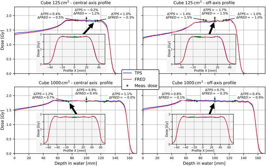
FIGURE 7. Longitudinal profiles across dose cubes along the central axis (left) and off-axis (right). The inlays show transverse profiles at the depth indicated by the arrow. Annotation boxes show relative difference between Fred/TPS and measurement at the indicated points.

They do not exceed 2%, and thus meet the clinical criteria.

3.2.4. Patient Quality Assurance

Figure 8 shows an example of a patient QA measurement and simulation (see Section 2.5.4). Simulations were performed with 10⁵ protons per spot on a single GPU card (Nvidia Titan Xp) and took a few minutes per QA plan. The resolution of the measured transverse dose map is limited by the 5 × 5 mm² pixel size of the detector. For TPS and Fred, a voxel size of 1 mm³ was used. The lower row shows the gamma index maps for the TPS and Fred vs. measurement, respectively. Accepted gamma index values are blue, while unacceptable ones are red. The gamma index (GI) passing rate (%GP), that is, the percent of pixels passing the GI test, is better comparing the Fred results to the measurements than the clinical TPS calculations. The lower right panel shows an example profile along the red line of the dose maps in the upper panel. The mean %GP out of the 10 measured transverse dose maps of this example treatment plan was 88.1 (4.1%) (Fred) and 80.6 (8.4%) (TPS). The results shown here are representative of all 300 simulated cases, and agreement of Fred with the TPS and data was always well within the clinically acceptable level.

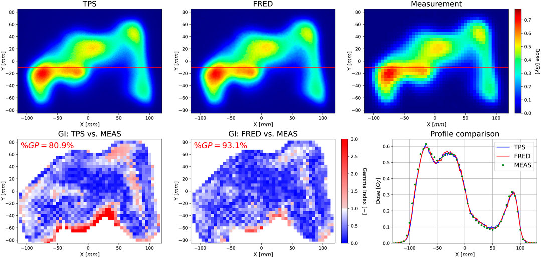
FIGURE 8. Transverse 2D dose distribution layer calculated by the TPS (upper left) obtained from Fred MC simulations (upper middle) and measured with an array of ionization chambers in the water phantom (upper right), as well as a GI map computed comparing the TPS (lower left) and Fred(lower middle) simulations to the measurement using the GI (2%/2 mm) method. The gamma passing rate (%GP) indicates the percent of pixels passing the GI test. The lower right panel shows dose profiles along the red line indicated on the upper panels.

3.3. Patient Simulations

Figure 9 shows a representative example of a full patient simulation performed with Fred and with the clinical TPS. The color wash figures present dose distributions recalculated in the patient geometry. Note that the clinical TPS (lower panels) masks the dose outside the patient contour. The treatment plan in this case includes three fields of pencil beams delivered under different angles. The upper right panel shows a profile across the patient volume (along the red line in the dose maps). The slight difference between the TPS and Fred at −190 mm to −170 mm is created by the lateral edge of the field coming from the upper left. We attribute this to differences in the CT calibration of lung tissue in Fred and the TPS which are currently under investigation. The lower right panel shows a dose volume histogram, that is, a cumulative distribution quantifying how many voxels within a certain geometrical region received at least a certain dose level. The match between the TPS and Fred is largely acceptable from a clinical point of view.

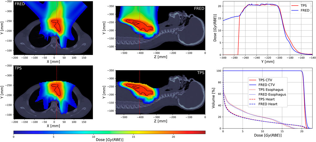
FIGURE 9. Dose distribution example (left and middle columns) of a patient treatment plan calculated with Fred MC (upper row) and the TPS (lower row) with a clinical target volume (CTV) structure marked with the black line, dose profiles (upper right) along the red dotted line indicated on the dose distribution panels, and comparison of dose volume histograms calculated for CTV and two selected organs at risk (lower right).

Simulations were performed with 10⁵ protons per spot on a single GPU card (Nvidia Titan Xp). Calculation times per treatment plan were about 25–30 min without and 10–15 min with the optimized geometry handling (cf. Section 2.3).

4. Discussion

We implemented the proton beam source of the therapeutic Mevion S250i proton accelerator in the Monte Carlo code Fred. This delivery system is more complex to implement than others because of the many degrees of freedom of the range modulation system and the adaptive aperture in the beam path which need to be considered. We chose to describe the pristine proton beam by a phase space model in a plane located at the scanning magnet position and to implement the geometry of the range modulation system and the adaptive aperture explicitly in Fred. Instead, we could have devised a phase space model at the exit of the beam nozzle without explicitly implementing the components. This would, however, have resulted in a very large phase space library because of the many degrees of freedom of the adaptive aperture and range modulator system. An interesting alternative to potentially investigate in the future would be the use of generative neural networks as recently proposed for phase space modeling of therapeutic linear accelerators [28]. We underline that Fred is not specific to the Mevion accelerator but can handle any other currently available proton therapy system if the beam line is properly implemented. For example, the therapeutic cyclotron of the proton therapy facility in Krakow has previously been implemented in Fred [29].

We modeled both the longitudinal and transverse components of the phase space model as Gaussian distributions characterized by their mean (which is zero for the transverse component) and variance. The motivation was mainly empirical, that is, it simply works in practice, and had been used in the past by other authors. A more refined model based on a detailed description and simulation of the full beam line would possibly deviate from a pure Gaussian distribution. On the other hand, the practical relevance of this is limited because scattering in the range shifter plates largely dominates the transverse beam shape. A pristine beam is rarely used in clinical treatment plans.

We chose to use an emittance model to describe the evolution of the beam size along the beam path from the virtual source plane to the beam nozzle. Another choice would have been a virtual point source model where the protons are all generated in a single point upstream of the exit window. Such a model generates a linearly divergent beam, and the opening angle is determined by the depth of the point source. From the theoretical point of view, the emittance model is more correct because it accounts for the correlation for the proton’s direction (momentum) and position in phase space. In fact, a proton beam can only have a waist (minimum of the emittance model), but not a point-like vertex, and a point source model thus gives an accurate representation of the beam only sufficiently far away from the waist. From the practical point of view, the transverse phase space model needs to be accurate only in the depth range where objects are present in the simulated geometry. According to Figure 3, the beam size evolves almost linearly in a range of about ±50 cm around the isocenter. In certain treatment configurations, however, the upstream surface of the nozzle region can be slightly more than 1 m away from the isocenter where the quadratic shape of the emittance model begins to be relevant. We therefore judge that the emittance model was a better choice in our case than a point source model.

Validation of the beam model was based on dose measurements and simulations because dose is the quantity of interest in a clinical application. Single pencil beams in water were used to assert the accuracy of the longitudinal phase space parameters and the parameterization of the range modulator plates. Validation based on dose layers and cubes showed that Fred correctly reproduced the superposition of pencil beams, both laterally and in depth as needed in patient treatments. Dose differences were on the level of 1–2% and met all the dosimetric criteria. In recalculated patient QA plans, Fred’s accuracy was at least as good as the clinical TPS when comparing simulation with measured data. Such a recalculation is an important use case for Fred, and we judge that our results justify its use as secondary dose engine for QA tasks. Full patient simulations, of which we showed a representative example here, also showed very good agreement between Fred and the clinical TPS.

Fred has initially been developed as a fast MC tool for dose calculation in particle therapy, and its functionality and physics models were implemented with this application in mind. Compared to general purpose MC codes, Fred has several limitations. First, only cuboid-shaped volumes can be defined. Other shapes, such as cylindrical detector devices, need to be approximated, for example, by a voxelized representation. Second, only voxel-based scorers are available, for example, to score dose, LET, or deposited energy on a grid. Scoring phase space properties (position and momentum) of individual particles, for example, is currently not available natively in Fred (but can be implemented by the user via plugins). Third, Fred tracks only those particles which are dosimetrically relevant on the scale of typical dose grids, that is, 1–2 mm. Specifically, Fred tracks secondary protons and deuterons, but lets heavier secondary particles deposit their energy locally because their range would anyhow be shorter than the voxel size. Neutrons and gamma rays are created, but not tracked, that is, they do not contribute to the deposited dose in the phantom. Some of this functionality is currently being developed and will probably be available in future versions of Fred.

A comparison of Fred with a general purpose of Monte Carlo software like Geant4 and FLUKA would have required a separate implementation of the Mevion system in these codes, which was clearly beyond the scope of this work. However, Fred’s proton tracking engine was validated against other codes and experimental data during the initial development of Fred [16]. From experiences with other proton therapy systems (unpublished), we know that Fred’s accuracy in clinical dose calculation is comparable to that of Geant4, while computation time is faster by orders of magnitude (minutes compared to tens of hours) at equal statistics.

A new functionality of Fred implemented as part of this work was the correct handling of situations where the beam nozzle overlaps with the volume containing the patient CT (cf. Section 2.3). It is worth noting that overlap of geometrical objects is a general difficulty encountered in most particle transport MC codes of our knowledge. In Geant4 (and derived applications) and FLUKA, for example, objects might be inserted into each other following a hierarchical child–parent structure, but partial overlap is not allowed, because the code would otherwise not be able to uniquely identify the object in which the particle needs to be traced. Geant4 provides a way to handle parallel geometries [30], which might be a starting point to handle overlapping volumes. Our implementation is not a general solution to the overlap problem. It works in this specific application because the beam nozzle is known to be the proton’s origin. Another solution would have been to use the outer patient surface as a boundary of the patient volume because overlap occurs only among those parts of the patient box containing air and not those containing tissue-filled voxels. Technically, however, this would have been much more difficult to handle because many parameters would be required to define such an irregular volume as opposed to a simple air-filled box enclosing the patient.

We conclude with a short discussion on the calculation times reported in the Results section for the different kinds of simulation. In particular, they were on the order of 10–15 min for full patient simulations which is largely sufficient for our main purpose of daily dose recalculation. Another measure of computational speed is the tracking time per proton, which was on the order of 3–5×10⁶ protons per second on the Nvidia Titan Xp card used in this work. This rate can only be reached if the card is optimally exploited, that is, if the number of primaries is large enough so that tracking is the dominant contribution compared to overhead due to data transfer to and from the GPU card. This was what prompted us to optimize the geometry handling in Fred in the first place (cf. Section 2.3), and indeed, calculation times improved by up to 70% for the full patient simulations. Furthermore, the number of protons per spot is currently set to a fixed number. A more elaborate scheme would set the number individually for each spot based on a requested noise level in the dose distributions, as it is implemented, for example, in the clinical TPS. Furthermore, no variance reduction techniques nor post-processing to de-noise the dose distributions are currently used in Fred (except for the fact that Fred is a condensed history code like all other general purpose Monte Carlo programs). All these methods are expected to improve calculation time even further.

5. Conclusion

We implemented a proton beam source for the Monte Carlo code Fred using a combination of the phase space model and explicit geometry of the beam nozzle components. The beam model was calibrated and validated by comparing measured and simulated data. The dosimetric accuracy was found to be sufficiently high to use Fred as the secondary dose calculator and at least as good as the clinical TPS.

Data Availability Statement

The raw data supporting the conclusions of this article will be made available by the authors, without undue reservation.

Ethics Statement

Ethical review and approval was not required for the study on human participants in accordance with the local legislation and institutional requirements. Written informed consent for participation was not required for this study in accordance with the national legislation and the institutional requirements.

Author Contributions

JG and IR developed and validated the beam model, and designed the project. JG, IR, and NK drafted the manuscript. IR and GV-F provided the experimental data and the technical information required to implement the beam model. AS and VP updated the FRED source code with the needed changes to perform this work. NK implemented the HU conversion in Fred. IR, AR, and VP provided their expertize in medical physics and in beam modeling. All the authors reviewed and approved the manuscript.

Funding

AR and JG acknowledged the Reintegration programme of the Foundation for Polish Science cofinanced by the EU under the European Regional Development Fund–grant no. POIR.04.04.00-00-2475/16-00.

Conflict of Interest

The authors declare that the research was conducted in the absence of any commercial or financial relationships that could be construed as a potential conflict of interest.

Acknowledgments

We would like to thank the commissioning team of the MAASTRO proton facility, that is, GV-F, Mirko Unipan, Jonathan Martens, Erik Roijen, and Geert Bosmans, for proving the measured data and for the fruitful discussions. We thank also Bas Nijsten for supporting this project. We gratefully acknowledge the support of NVIDIA Corporation with the donation of the GPU cards used for this research.

References

1. Beltran C, Tseung HWC, Augustine KE, Bues M, Mundy DW, Walsh TJ, et al. Clinical implementation of a proton dose verification system utilizing a GPU accelerated Monte Carlo engine. Int J Part Ther (2016) 3:312–9. doi:10.14338/IJPT-16-00011.1
2. Meijers A, Guterres Marmitt G, Ng Wei Siang K, van der Schaaf A, Knopf AC, Langendijk JA, et al. Feasibility of patient specific quality assurance for proton therapy based on independent dose calculation and predicted outcomes. Radiother Oncol (2020) 150:136–41. doi:10.1016/j.radonc.2020.06.027
3. Paganetti H, Jiang H, Parodi K, Slopsema R, Engelsman M. Clinical implementation of full Monte Carlo dose calculation in proton beam therapy. Phys Med Biol (2008) 53:4825–53. doi:10.1088/0031-9155/53/17/023
4. Paganetti H Range uncertainties in proton therapy and the role of Monte Carlo simulations. Phys Med Biol (2012) 57:R99–117. doi:10.1088/0031-9155/57/11/R99
5. Battistoni G, Boccone V, Boehlen T, Broggi F, Brugger M, Brunetti G, et al. FLUKA Monte Carlo calculations for hadrontherapy application. 13th international conference on nuclear reaction mechanisms, 2012 January 11–15; Varenna, Italy. Geneva: CERN (2013). p. 461.
6. Böhlen TT, Cerutti F, Dosanjh M, Ferrari A, Gudowska I, Mairani A, et al. Benchmarking nuclear models of FLUKA and GEANT4 for carbon ion therapy. Phys Med Biol (2010) 55:5833–47. doi:10.1088/0031-9155/55/19014
7. Parodi K, Mairani A, Brons S, Hasch BG, Sommerer F, Naumann J, et al. Monte Carlo simulations to support start-up and treatment planning of scanned proton and carbon ion therapy at a synchrotron-based facility. Phys Med Biol 57 (2012) 3759–84. doi:10.1088/0031-9155/57/12/3759
8. Henkner K, Sobolevsky N, Jäkel O, Paganetti H. Test of the nuclear interaction model in SHIELD-HIT and comparison to energy distributions from GEANT4. Phys Med Biol 54 (2009) N509–17. doi:10.1088/0031-9155/54/22/n01
9. Agostinelli S, Allison J, Amako K, Apostolakis J, Araujo H, Arce P, et al. GEANT4– a simulation toolkit. Nucl Instrum Methods Phys Res, Sect A (2003) 506:250–303. doi:10.1016/S0168-9002(03)01368-8
10. Santin G, Staelens S, Taschereau R, Descourt P, Schmidtlein CR, Simon L, et al. Evolution of the GATE project: new results and developments. Nucl Phys B Proc Suppl (2007) 172:101–3. doi:10.1016/j.nuclphysbps.2007.07.008
11. Sarrut D, Bardiès M, Boussion N, Freud N, Jan S, Létang JM, et al. A review of the use and potential of the GATE Monte Carlo simulation code for radiation therapy and dosimetry applications. Med Phys (2014) 41:1–14. doi:10.1118/1.4871617
12. Perl J, Shin J, Schümann J, Faddegon B, Paganetti H. TOPAS: an innovative proton Monte Carlo platform for research and clinical applications. Med Phys (2012) 39:6818–38. doi:10.1118/1.4758060
13. Testa M, Schümann J, Lu HM, Shin J, Faddegon B, Perl J, et al. Experimental validation of the TOPAS Monte Carlo system for passive scattering proton therapy. Med Phys (2013) 40:121719. doi:10.1118/1.4828781
14. Jia X, Schümann J, Paganetti H, Jiang SB. GPU-based fast Monte Carlo dose calculation for proton therapy. Phys Med Biol (2012) 57:7783–97. doi:10.1088/0031-9155/57/23/7783
15. Qin N, Botas P, Giantsoudi D, Schuemann J, Tian Z, Jiang SB., et al. Recent developments and comprehensive evaluations of a GPU-based Monte Carlo package for proton therapy. Phys Med Biol (2016) 61:7347–62. doi:10.1088/0031-9155/61/20/7347
16. Schiavi A, Senzacqua M, Pioli S, Mairani A, Magro G, Molinelli S, et al. Fred: a GPU-accelerated fast-Monte Carlo code for rapid treatment plan recalculation in ion beam therapy. Phys Med Biol (2017) 62:7482–504. doi:10.1088/1361-6560/aa8134
17. Wan Chan Tseung H, Ma J, Beltran C. A fast GPU-based Monte Carlo simulation of proton transport with detailed modeling of nonelastic interactions. Med Phys (2015) 42:2967–78. doi:10.1118/1.4921046
18. Mein S, Choi K, Kopp B, Tessonnier T, Bauer J, Ferrari A, et al. Fast robust dose calculation on GPU for high-precision 1H, 4He, 12C and 16O ion therapy: the FRoG platform. Sci Rep (2018) 8:14829. doi:10.1038/s41598-018-33194-4
19. Grevillot L, Bertrand D, Dessy F, Freud N, Sarrut D. A Monte Carlo pencil beam scanning model for proton treatment plan simulation using GATE/GEANT4. Phys Med Biol (2011) 56:5203–19. doi:10.1088/0031-9155/56/16/008
20. Grevillot L, Bertrand D, Dessy F, Freud N, Sarrut D. GATE as a GEANT4-based Monte Carlo platform for the evaluation of proton pencil beam scanning treatment plans. Phys Med Biol (2012) 57:4223–44. doi:10.1088/0031-9155/57/13/4223
21. Paganetti H, Jiang H, Lee SY, Kooy HM. Accurate Monte Carlo simulations for nozzle design, commissioning and quality assurance for a proton radiation therapy facility. Med Phys (2004) 31:2107–18. doi:10.1118/1.1762792
22. Cirrone G, Cuttone G, Guatelli S, Lo Nigro S, Mascialino B, Pia M, et al. Implementation of a new Monte Carlo-GEANT4 Simulation tool for the development of a proton therapy beam line and verification of the related dose distributions. IEEE Trans Nucl Sci (2005) 52:262–5. doi:10.1109/TNS.2004.843140
23. Prusator M, Ahmad S, Chen Y. TOPAS Simulation of the Mevion S250 compact proton therapy unit. J Appl Clin Med Phys (2017) 18:88–95. doi:10.1002/acm2.12077
24. Vilches-Freixas G, Unipan M, Rinaldi I, Martens J, Roijen E, Almeida IP, et al. Beam commissioning of the first compact proton therapy system with spot scanning and dynamic field collimation. Br J Radiol (2020) 93:20190598. doi:10.1259/bjr.20190598
25. Twiss RQ,, Frank NH. Orbital stability in a proton synchrotron. Rev Sci Instrum (1949) 20:1–17. doi:10.1063/1.1741343
26. Bortfeld T,, Schlegel W. An analytical approximation of depth - dose distributions for therapeutic proton beams. Phys Med Biol (1996) 41:1331–9. doi:10.1088/0031-9155/41/8/006
27. Kanematsu N, Inaniwa T, Nakao M. Modeling of body tissues for Monte Carlo simulation of radiotherapy treatments planned with conventional x-ray CT systems. Phys Med Biol (2016) 61:5037–50. doi:10.1088/0031-9155/61/13/5037
28. Sarrut D, Krah N, Létang JM. Generative adversarial networks (GAN) for compact beam source modelling in Monte Carlo simulations. Phys Med Biol (2019) 64:215004. doi:10.1088/1361-6560/ab3fc1
29. Garbacz M, Battistoni G, Durante M, Gajewski J, Krah N, Patera V, et al. Proton therapy treatment plan verification in CCB Krakow using fred Monte Carlo TPS tool. In: L Lhotska, L Sukupova, I Lacković, and GS Ibbott, editors World congress on medical physics and biomedical engineering 2018. Singapore: Springer Singapore (2019). p. 783–7.
Keywords: proton therapy, Monte Carlo dose calculation, GPU-accelerated dose calculation, phase space modelling, pencil beam scanning, quality assurance
Citation: Gajewski J, Schiavi A, Krah N, Vilches-Freixas G, Rucinski A, Patera V and Rinaldi I (2020) Implementation of a Compact Spot-Scanning Proton Therapy System in a GPU Monte Carlo Code to Support Clinical Routine. Front. Phys. 8:578605. doi: 10.3389/fphy.2020.578605
Received: 30 June 2020; Accepted: 04 November 2020;
Published: 23 December 2020.
Edited by:
Anna Vignati, University of Turin, ItalyReviewed by:
Jacobo Cal-Gonzalez, Ion Beam Applications (Spain), SpainLorenzo Manganaro, aizoOn Technology Consulting, Italy
Copyright © 2020 Gajewski, Schiavi, Krah, Vilches-Freixas, Rucinski, Patera and Rinaldi. This is an open-access article distributed under the terms of the Creative Commons Attribution License (CC BY). The use, distribution or reproduction in other forums is permitted, provided the original author(s) and the copyright owner(s) are credited and that the original publication in this journal is cited, in accordance with accepted academic practice. No use, distribution or reproduction is permitted which does not comply with these terms.
*Correspondence: Ilaria Rinaldi, ilaria.rinaldi@maastro.nl