Investigations on Average Fluorescence Lifetimes for Visualizing Multi-Exponential Decays

Li, Yahui; Natakorn, Sapermsap; Chen, Yu; Safar, Mohammed; Cunningham, Margaret; Tian, Jinshou; Li, David Day-Uei

doi:10.3389/fphy.2020.576862

ORIGINAL RESEARCH article

Front. Phys., 16 October 2020
Sec. Optics and Photonics
Volume 8 - 2020 | https://doi.org/10.3389/fphy.2020.576862

Investigations on Average Fluorescence Lifetimes for Visualizing Multi-Exponential Decays

Yahui Li^1,2,3

Sapermsap Natakorn⁴

Yu Chen⁴

Mohammed Safar¹

Margaret Cunningham¹

Jinshou Tian^2,3

David Day-Uei Li¹^*

¹Strathclyde Institute of Pharmacy and Biomedical Sciences, University of Strathclyde, Glasgow, United Kingdom
²Key Laboratory of Ultra-fast Photoelectric Diagnostics Technology, Xi'an Institute of Optics and Precision Mechanics, Xi'an, China
³University of Chinese Academy of Sciences, Beijing, China
⁴Department of Physics, Scottish Universities Physics Alliance, University of Strathclyde, Glasgow, United Kingdom

Intensity- and amplitude-weighted average lifetimes, denoted as τ_I and τ_A hereafter, are useful indicators for revealing Förster resonance energy transfer (FRET) or fluorescence quenching behaviors. In this work, we discussed the differences between τ_I and τ_A and presented several model-free lifetime determination algorithms (LDA), including the center-of-mass, phasor, and integral equation methods for fast τ_I and τ_A estimations. For model-based LDAs, we discussed the model-mismatch problems, and the results suggest that a bi-exponential model can well approximate a signal following a multi-exponential model. Depending on the application requirements, suggestions about the LDAs to be used are given. The instrument responses of the imaging systems were included in the analysis. We explained why only using the τ_I model for FRET analysis can be misleading; both τ_I and τ_A models should be considered. We also proposed using τ_A/τ_I as a new indicator on two-photon fluorescence lifetime images, and the results show that τ_A/τ_I is an intuitive tool for visualizing multi-exponential decays.

1. Introduction

Fluorescence lifetime imaging (FLIM) is a crucial technique for assessing microenvironments of fluorescent molecules [1, 2], such as pH [3], Ca²⁺ [4, 5], O₂ [6], viscosity [7], or temperature [8]. Combining with Förster Resonance Energy Transfer (FRET) techniques, FLIM can be a powerful “quantum ruler” to measure protein conformations and interactions [9–12]. Compared with fluorescence intensity imaging, FLIM is independent of the signal intensity and fluorophore concentrations, making FLIM a powerful quantitative imaging technique for applications in life sciences [13], medical diagnosis [14–16], drug developments [17–19], and flow diagnosis [20–22]. FLIM techniques can build on time-correlated single-photon counting (TCSPC) [23–25], time-gating [26–28], or streak cameras [29]; they record time-resolved fluorescence intensity profiles to extract lifetimes with a lifetime determination algorithm (LDA) [1]. There is a rapid growth of real-time applications that fast analysis is sought after [12, 30]. Traditional LDAs usually use the least square method (LSM) or maximum likelihood estimation (MLE) [31] to analyze decay models chosen by users, and model-fitting analysis follows a reduced chi-squared criterion [1]. In reality, however, it is difficult to know the exact decay model as fluorescent molecules in biological systems can demonstrate complex multi-exponential decay profiles. For instance, a mixture of fluorophores, a multi-tryptophan protein, single fluorophores in varied environments, and single-tryptophan proteins in multiple conformational states [1] can show multi-exponential decays as

\begin{array}{l} f (t) = A \sum_{i = 1}^{p} q_{i} exp (- t / τ_{i}), where \sum_{i = 1}^{p} q_{i} = 1, & (1) \end{array}

where A represents the amplitude, q_i and τ_i (i = 1, …, p) denote the amplitude fractions and lifetimes, respectively, and p is the number of lifetime components. There are time-domain or frequency-domain [32–35] FLIM systems to measure a fluorescence decay. In this work, we focus on time-domain approaches.

Suppose the instrument response function (IRF) of the measurement system is irf(t), the task performed by FLIM analysis tools is to extract f(t) from the measured decay h(t), as

\begin{array}{l} h (t) = i r f (t) * f (t) . & (2) \end{array}

The problems with traditional LSM or MLE are two-fold. (1) It is challenging to categorize a fluorescence emission into a specific exponential model described by Equation (1) in complex biological processes. An arbitrary choice of p in Equation (1) simply based on reduced chi-squared tests [36] would lead to totally different interpretations. As the fitting routine is not mathematically unique; a measured decay could be fitted equally well with a bi-exponential or a tri-exponential model. (2) To ensure the accuracy, it usually needs a high photon count (long acquisition time) when p ≥ 2 [37]. Instead of completely extracting q_i and τ_i (i = 1, …, p), which is doubtful as mentioned above and time-consuming, in many applications, it is often useful to determine only the average lifetime which can be expressed in two forms [1]: the intensity-weighted average lifetime

\begin{array}{l} τ_{I} = \sum_{i = 1}^{p} q_{i} τ_{i}^{2} / \sum_{i = 1}^{p} q_{i} τ_{i}, & (3) \end{array}

and the amplitude-weighted average lifetime

\begin{array}{l} τ_{A} = \sum_{i = 1}^{p} q_{i} τ_{i} / \sum_{i = 1}^{p} q_{i} = \sum_{i = 1}^{p} q_{i} τ_{i} . & (4) \end{array}

The question about which average lifetime we should use according to the applications has been investigated in [38]. For instance, they suggested:

(a) τ_A can estimate the energy transfer efficiency in FRET [39],

\begin{array}{l} E = 1 - \frac{I_{D A}}{I_{D}} = 1 - \frac{τ_{D A, A}}{τ_{D, A}}, & (5) \end{array}

where E is the energy transfer efficiency, I_DA and I_D are the fluorescence intensities of the donor in the presence and absence of energy transfer, respectively, and τ_{DA, A} and τ_{D, A} are τ_A of the donor in the presence and absence of energy transfer, respectively. E can further estimate the donor-acceptor distance.

(b) τ_A can also assess dynamic quenching behaviors, described by the Stern-Volmer equation [40],

\begin{array}{l} \frac{I_{0}}{I_{1}} = 1 + K_{D} [Q] = \frac{τ_{0, A}}{τ_{1, A}}, & (6) \end{array}

where I₀ and I₁ are fluorescence intensities, τ_{0, A} and τ_{1, A} are τ_A of the fluorophore in the absence and presence of the quencher, respectively, K_D is the Stern-Volmer quenching constant, and [Q] is the concentration of the quencher. Additionally, the average radiative rate constant can be expressed as, k_r = QE/τ_{1, A}, where QE is the quantum yield.

Average lifetimes can either be calculated by extracting the lifetime components using model-based LDAs and then using Equations (3) and (4). Or they can be directly obtained with model-free LDAs, such as hardware-friendly center-of-mass methods (CMM) [41–44], the phasor method (Phasor) [45–47], the rapid lifetime determination method (RLD) [30, 48–51], or the integral extraction method (IEM) [52, 53], without assuming any decay model.

In this work, we theoretically investigated two types of average lifetimes evaluated by model-free LDAs, examined the performances of τ_A and τ_I estimations using different LDAs, and suggested the choices of LDAs in terms of accuracy, precision, and estimation speeds according to the applications. We also described a multi-exponential decay visualization tool using the ratio τ_A/τ_I. Experimental results demonstrate the performance of τ_A/τ_I in comparison with Phasor.

2. Theory

In this section, we derived the average lifetimes determined by the model-free methods, CMM, Phasor, and IEM and described the general work flow of average lifetime estimations with the model-free and model-based LDAs.

As Equation (2), the measured signal h(t) is the convolution of f(t) with irf(t). Here we focus on the signal h_m and irf_m obtained from a TCSPC system, as shown in Figure 1,

\begin{array}{l} h_{m} = \sum_{k = 0}^{m} i r f_{k - m} \cdot f_{m}, m = 0, 1, 2, \dots, M - 1, \\ i r f_{m} = \int_{m Δ t}^{(m + 1) Δ t} i r f (t) d t, \\ f_{m} = \int_{m Δ t}^{(m + 1) Δ t} f (t) d t = A \sum_{i = 1}^{p} q_{i} τ_{i} e^{- \frac{m Δ t}{τ_{i}}} [1 - e^{- \frac{Δ t}{τ_{i}}}], & (7) \end{array}

where h_m is the photon count collected in Bin m at t_m = (m + 1/2)Δt, M is the number of bins, and Δt is the time resolution.

FIGURE 1

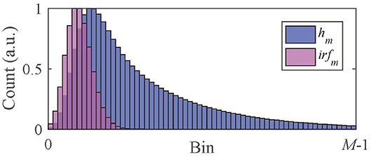
Figure 1. Illustration of h_m and irf_m obtained with a TCSPC system.

(a) CMM

The average lifetime evaluated with CMM is

\begin{array}{l} τ_{C M M} = \frac{\int_{0}^{\infty} t \cdot h (t) d t}{\int_{0}^{\infty} h (t) d t} - \frac{\int_{0}^{\infty} t \cdot i r f (t) d t}{\int_{0}^{\infty} i r f (t) d t} = \frac{\sum_{i = 1}^{p} q_{i} τ_{i}^{2}}{\sum_{i = 1}^{p} q_{i} τ_{i}} \\ ≃ \frac{\sum_{m = 0}^{M - 1} t_{m} \cdot h_{m}}{\sum_{m = 0}^{M - 1} h_{m}} - \frac{\sum_{m = 0}^{M - 1} t_{m} \cdot i r f_{m}}{\sum_{m = 0}^{M - 1} i r f_{m}}, & (8) \end{array}

which is equal to τ_I. The derivation of Equation (8) is shown in the Appendix.

(b) Phasor

The average lifetime evaluated with Phasor is

\begin{array}{l} τ_{P} = \frac{s}{g ω} = \frac{\sum_{i = 1}^{p} q_{i} τ_{i}^{2} / (1 + ω^{2} τ_{i}^{2})}{\sum_{i = 1}^{p} q_{i} τ_{i} / (1 + ω^{2} τ_{i}^{2})}, & (9) \end{array}

where ω = 2π/T, T = MΔt is the measurement window, and g and s are the phasor components expressed as

\begin{array}{l} g = \frac{\int_{0}^{\infty} f (t) \cdot cos (ω t) d t}{\int_{0}^{\infty} f (t) d t} = \frac{\sum_{i = 1}^{p} q_{i} τ_{i} / (1 + ω^{2} τ_{i}^{2})}{\sum_{i = 1}^{p} q_{i} τ_{i}} \\ = \frac{R_{h} + s \cdot I_{i r f}}{R_{i r f}}, \\ s = \frac{\int_{0}^{\infty} f (t) \cdot sin (ω t) d t}{\int_{0}^{\infty} f (t) d t} = \frac{\sum_{i = 1}^{p} ω q_{i} τ_{i}^{2} / (1 + ω^{2} τ_{i}^{2})}{\sum_{i = 1}^{p} q_{i} τ_{i}} \\ = \frac{I_{h} \cdot R_{i r f} - R_{h} \cdot I_{i r f}}{R_{i r f}^{2} + I_{i r f}^{2}}, \end{array}

where

\begin{array}{l} R_{h} = \frac{\int_{0}^{\infty} h (t) \cdot cos (ω t) d t}{\int_{0}^{\infty} h (t) d t} ≃ \frac{\sum_{m = 0}^{M - 1} h_{m} \cdot cos (ω t_{m})}{\sum_{m = 0}^{M - 1} h_{m}}, \\ I_{h} = \frac{\int_{0}^{\infty} h (t) \cdot sin (ω t) d t}{\int_{0}^{\infty} h (t) d t} ≃ \frac{\sum_{m = 0}^{M - 1} h_{m} \cdot sin (ω t_{m})}{\sum_{m = 0}^{M - 1} h_{m}}, \end{array}

\begin{array}{l} R_{i r f} = \frac{\int_{0}^{\infty} i r f (t) \cdot cos (ω t) d t}{\int_{0}^{\infty} i r f (t) d t} ≃ \frac{\sum_{m = 0}^{M - 1} i r f_{m} \cdot cos (ω t_{m})}{\sum_{m = 0}^{M - 1} i r f_{m}}, \\ I_{i r f} = \frac{\int_{0}^{\infty} i r f (t) \cdot sin (ω t) d t}{\int_{0}^{\infty} i r f (t) d t} ≃ \frac{\sum_{m = 0}^{M - 1} i r f_{m} \cdot sin (ω t_{m})}{\sum_{m = 0}^{M - 1} i r f_{m}} . \end{array}

τ_P is a weighted average lifetime whose weights are $q_{i} τ_{i} / (1 + ω^{2} τ_{i}^{2})$ . If τ_i ≪ T, then the weights are approximately equal to q_iτ_i, i.e., τ_P is close to τ_I.

For IEM, the underlying exponential decay should be extracted by a model-free deconvolution method. With the estimated exponential decay ${\hat{f}}_{m}$ , the average lifetime with IEM is

\begin{array}{l} τ_{I E M} = - \frac{\int_{0}^{\infty} g (t) d t}{\int_{0}^{\infty} g^{'} (t) d t} = \frac{\sum_{i = 1}^{p} q_{i} τ_{i}}{\sum_{i = 1}^{p} q_{i}} ≃ - \frac{Δ t \sum_{m = 0}^{M - 1} S_{m} \cdot {\hat{f}}_{m}}{{\hat{f}}_{M - 1} - {\hat{f}}_{0}}, \\ g (t) = A \sum_{i = 1}^{p} q_{i} τ_{i} e^{- t / τ_{i}} [1 - e^{- Δ t / τ_{i}}], & (10) \end{array}

where S_m = [1/3, 4/3, 2/3, 4/3, 1/3] are the coefficients for numerical integration based on Simpson's rule. τ_IEM is actually an estimator for τ_A.

Figure 2 summarizes the flow diagram for τ_I and τ_A estimations with different algorithms used in this study. The simulated signals h_m and irf_m are directly sent into CMM and Phasor blocks to estimate τ_I. The estimated f_m (from h_m and irf_m with the Laguerre expansion deconvolution method with L = 16 and α = 0.912 [54, 55]) is sent to IEM to estimate τ_A and sent to the bi-decay center-of-mass method (BCMM; j = 2) [56], the variable projection method (VPM; j = 2) [57], or LSM with a j-exponential model (denoted as LSM-j), to estimate τ_I and τ_A. CMM and Phasor are fast as no deconvolution routine is needed, whereas IEM, BCMM, VPM, and LSM are direct or iterative estimation approaches once f_m is extracted. Artificial neural network assisted analysis tools [58, 59] can be included in this diagram, but they are out of the scope of this work.

FIGURE 2

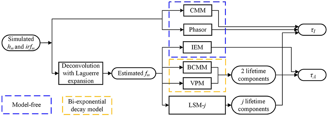
Figure 2. Flow diagram for τ_I and τ_A estimations.

3. Results

3.1. Simulations

In reality, it is difficult to characterize a real fluorescence profile with a suitable exponential model described in Equation (1). To demonstrate how model-free analysis can be beneficial, we examined two scenarios. Case A: we used exponential decay signals with p = 1 ~ 4 to assess the influence of the model mismatch between the signal and the algorithm on τ_I and τ_A estimations. This study is to investigate the scenario when users select a j-exponential model to analyze a p-exponential decay (p can be different from j). Case B: we generated synthetic bi-exponential (p = 2) decay signals to assess the performances of τ_I and τ_A estimations with the model-free and model-based LDAs.

The performances of lifetime estimations can be assessed in two aspects: (1) the accuracy $B_{n} = | {\hat{τ}}_{n} - τ_{n} | / τ_{n}$ and the precision $F_{n} = \sqrt{N_{t o t}} σ_{{\hat{τ}}_{n}} / {\hat{τ}}_{n}$ [60], where n = I or A for the intensity- or the amplitude-weighted lifetimes, τ_n and ${\hat{τ}}_{n}$ are actual and estimated values, $σ_{{\hat{τ}}_{n}}$ is the standard deviation of ${\hat{τ}}_{n}$ , and N_tot is the total photon count. The lower the F, the higher the precision (F = 1 for the ideal case).

3.1.1. Case A: Model Mismatch

Ideally, a bi-exponential signal should be analyzed by a bi-exponential model. For instance, BCMM, VPM, and LSM-2 are used for bi-exponential decay models, and LSM-j for j-exponential models, j > 2. However, in realistic biological processes, it is difficult to know precisely how many lifetime components a decay profile contains. In traditional FLIM analysis tools, users usually need to select an exponential model to fit measured decays and use the reduced chi-squared to evaluate the goodness-of-fit. If the reduced chi-squared is not satisfactory, then a different exponential model is chosen. This process continues until the reduced chi-squared is acceptable. Often different exponential models can produce similar reduced chi-squared values, and the question is which fitting we should use? It is quite common that a j-exponential model might analyze a signal containing p lifetime components and j ≠ p. We would like to know if p is unknown to the user, whether using a different analysis model (j ≠ p) would lead to a different biological story.

We generated exponential decay signals h_m (m = 0,…, M-1) to test the LDAs for τ_I and τ_A estimations. h_m can be artificially generated with $f (t) = A \sum_{i = 1}^{p} q_{i} exp (- t / τ_{i})$ , where p = [1, 2, 3, 4], q_i = 1/p, and the IRF is approximated with a Poisson distribution $i r f_{m} = exp (λ) λ^{m} / m!$ with λ = 500 ps, FWHM ≃ 300 ps, and M = 256. The measurement window T = 10 ns, and the total photon count N_tot = 10³. τ_i, τ_I, and τ_A for each p are summarized in Table 1.

TABLE 1

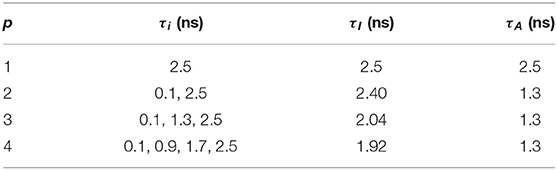
Table 1. τ_i, τ_I, and τ_A for p = 1 ~ 4 with q_i = 1/p.

The performances of τ_I and τ_A estimations with the simulated exponential decays are shown in Figures 3A–D for B_I, F_I, B_A, and F_A, respectively. For model-free LDAs, B_I and B_A are below 10% and are independent of p. For LSM-1, when p = 1, B_I, and B_A are zero, whereas when p > 1, B_I and B_A increase especially for p = 2. For model-based LDAs where j > 1, BCMM, VPM, and LSM-j have similar performances even for p ≠ j, seemingly suggesting that a bi-exponential model can well approximate a signal following an arbitrary p-exponential model. We generated 100 signals with τ_i and q_i chosen randomly in the ranges of 0.1 ~ 2.5 ns and 0.1 ~ 0.9, respectively, for each p. BCMM, VPM, and LSM-2 were used to fit the signals with bi-exponential decays. The goodness-of-fit is judged by the reduced chi-squared $χ^{2} = \frac{1}{M} \sum_{m = 0}^{M - 1} {(f_{m} - f_{c, m})}^{2} / f_{m}$ , where f_m and f_{c, m} are actual and fitted signals of Bin m. The box plots of χ² for BCMM, VPM, and LSM-2 are shown in Figures 3E–G, respectively. The χ² values are insensitive to p for the three LDAs so that we conclude that a bi-exponential decay is suitable to approximate an arbitrary p-exponential decay (p ≤ 4).

FIGURE 3

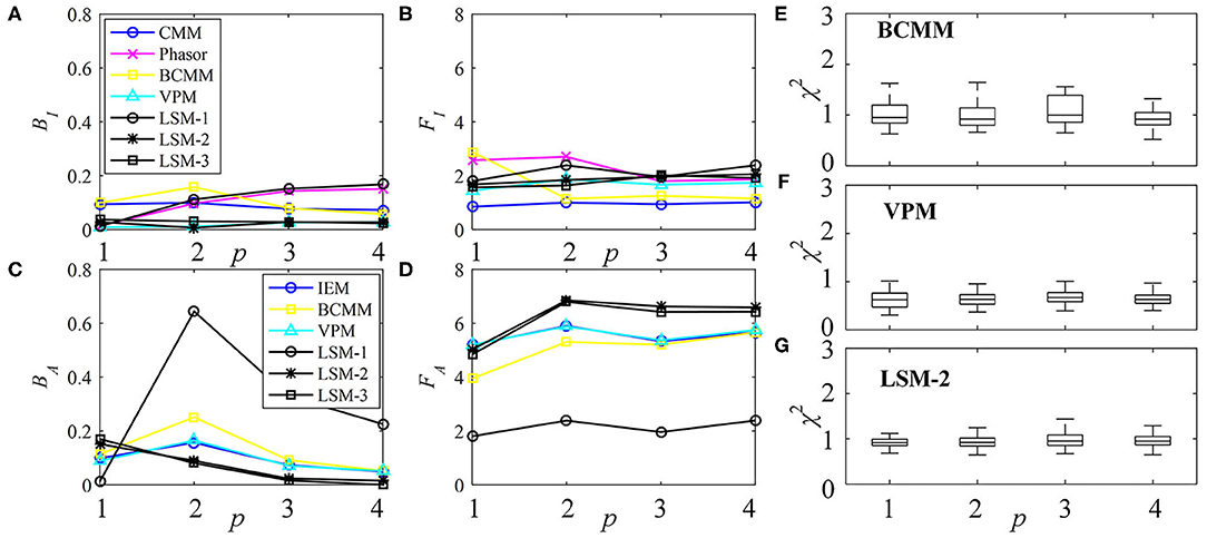
Figure 3. Performances of τ_I and τ_A estimations with exponential decay signals using different algorithms, (A) B_I, (B) F_I, (C) B_A, and (D) F_A. (E–G) Box plots of χ² for BCMM, VPM, and LSM-2.

Therefore, if the decay model of the signal is inaccessible, model-free and model-based LDAs, BCMM, VPM, and LSM-2 are enough for τ_I and τ_A estimations.

In practice, users can choose an optimization algorithm and set initial conditions to analyze FLIM images when LSM-2 is used. We would like to know how they can affect τ_I and τ_A estimations. Four bi-exponential decays, Decays 1 ~ 4, with different parameters (q₁, τ₁, τ₂) were analyzed using LSM-2 with different initial conditions (q₁₀, τ₁₀, τ₂₀), denoted as Init. 1 ~ 4 listed in Table 2 with N_tot = 10³. When either of the estimated τ₁ and τ₂ is larger than T (10 ns), we say that the estimation fails. The probabilities of producing a failed trial, P(τ₁ or τ₂ > 10) and producing biased τ_I and τ_A with B_I and B_A > 0.3, i.e., P(B_n > 0.3), n = I or A, are shown in Figure 4. Figures 4A–F are the LSM-2 results with the unconstrained and constrained trust-region-reflective (TRR) algorithms, respectively. The constraints are 0 < q₁ < 1 and 0 < τ₁, τ₂ < 10 ns. Figures 4G–I are the LSM-2 results using the Levenberg-Marquardt (LM) algorithm. For the unconstrained TRR, the performances are relatively sensitive to initial conditions. P(τ₁ or τ₂ > 10) for Init. 4 is quite significant which results in large P(B_n > 0.3), n = I or A, for all four decays. Although Init. 3 leads to a low P for Decays 2 ~ 3, P(B_A > 0.3) for Decay 1 rises to 0.7. Thus, if the initial conditions are not chosen properly, the quality of τ_I and τ_A images cannot be guaranteed. The constrained TRR and LM are insensitive to initial conditions. Although the LM has failed trials, they barely affect P(B_n > 0.3), n = I or A. Therefore, to ensure accurate τ_I and τ_A estimations, the constrained TRR and LM are recommended for LSM-2.

TABLE 2

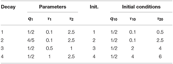
Table 2. Bi-exponential decays and initial conditions for τ_I and τ_A estimations with LSM-2.

FIGURE 4

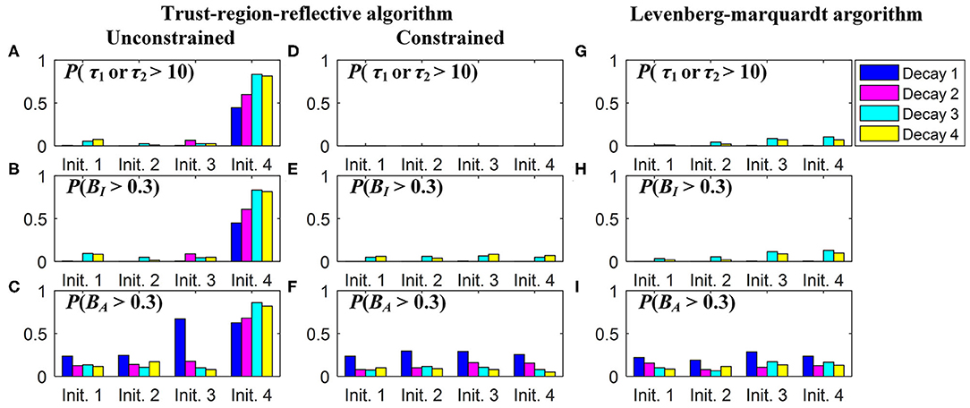
Figure 4. (A,D,G) P(τ₁ or τ₂ > 10), (B,E,H) P(B_I > 0.3), and (C,F,I) P(B_A > 0.3), for estimations of Decays 1 ~ 4 with Init. 1 ~ 4 using (A–C) the unconstrained TRR, (D–F) the constrained TRR, and (G–I) the LM algorithms.

3.1.2. Case B: Performances of Average Lifetime Estimations

As mentioned above, it might be challenging to use a proper exponential model to describe realistic biological processes; a bi-exponential model might well approximate them. Here we will use a bi-exponential model to explain why model-free LDAs have the benefits of higher photon efficiency and faster analysis than model-based LDAs for τ_I and τ_A estimations.

h_m can be artificially generated with the same IRF used in Case A and f(t) = A[q₁exp(−t/τ₁) + (1 − q₁)exp(−t/τ₂)], where τ₁ < τ₂ and q₁ is the amplitude fraction of τ₁. Figure 5A shows the signal and IRF. In FRET and dynamic quenching applications, the fluorescence lifetime of the donor fluorophore is in general decreasing, and we assume τ₂ = 2.5 ns and τ₁ varying from 0.1 to 2.5 ns to emulate FRET or quenching. The theoretical τ_I, τ_A, and τ_P with q₁ = 0.5 are shown in Figure 5B. τ_P has a negative bias from τ_I. With T/τ₂ increasing, τ_P approaches τ_I. Figure 5B that two different (τ₁, τ₂) sets can deliver the same τ_I, for instance, (0.32, 2.5) ns and (2.1, 2.5) ns have the same τ_I of 2.3 ns.

FIGURE 5

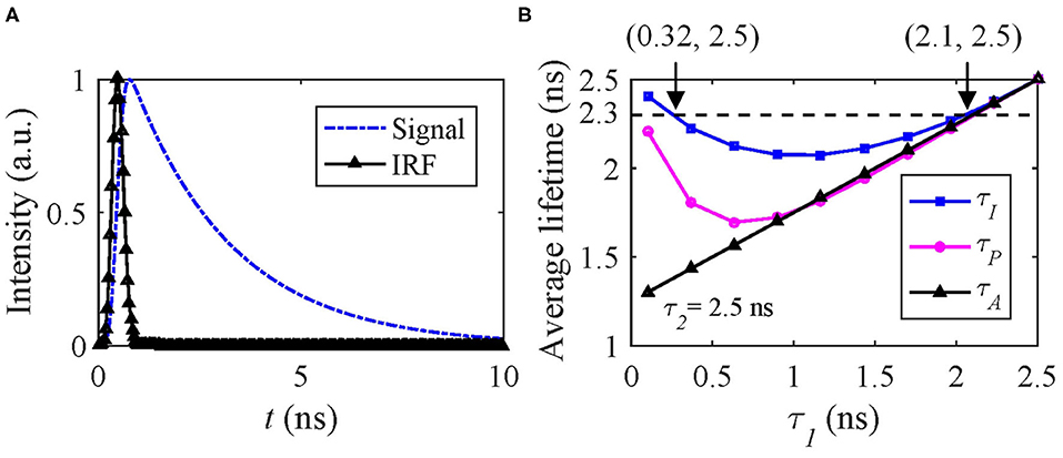
Figure 5. (A) Simulated signal (blue) and IRF (black), (B) theoretical τ_I (blue), τ_A (black), and τ_P (magenta) average lifetimes with q₁ = 0.5.

Therefore, only estimating τ_I can be misleading. Figure 5B also shows that the dynamic range of τ_I is only 2.5–2.23 = 0.27 ns and within which the above problem persists. Whereas τ_A does not have this problem for this case. We conducted Monte Carlo simulations to estimate τ_I and τ_A with the simulated signals, including Poisson noise under different conditions q₁ = 0.2, 0.5, and 0.8.

The performances of τ_I and τ_A estimations with bi-exponential decay signals are shown in Figures 6A–D for B_I, F_I, B_A, and F_A, respectively. For ${\hat{τ}}_{I}$ , B_{I, CMM}, and B_{I, BCMM} are roughly 10 and 8%, respectively determined by T/τ₂. The larger T/τ₂ is, the smaller B_I becomes (with F_{I, CMM} and F_{I, BCMM} being closer to 1). Phasor has a lower accuracy when q₁ becomes larger and τ₁ smaller, and it is less precise than CMM. VPM and LSM-2 both have a smaller B_I = 3% but higher F_I (1.5 ~ 5) than CMM and BCMM. For ${\hat{τ}}_{A}$ , B_A is 7% except for τ₁ = 0.1 ns, and F_A is around 5 for the four LDAs. Figures 6C,D show that if only τ_A is needed, there is no need to resort to slower model-based LDAs.

FIGURE 6

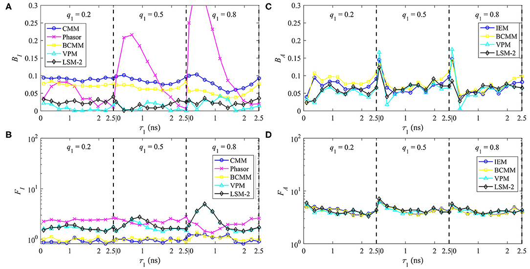
Figure 6. The performances of τ_I and τ_A estimations with bi-exponential decay signals with τ₁ = 0.1 ~ 2.5 ns, τ₂ = 2.5 ns, q₁ = 0.2, 0.5, 0.8, (A) B_I, (B) F_I and (C) B_A, (D) F_A.

For τ_I estimations, LSM-2 and VPM are preferred when high accuracy is required. Still, they are slower and have lower photon efficiency than CMM and BCMM which means the photon count should be higher to have similar precision, for instance, a relative standard deviation of 5% can be reached with N_tot = 3,600 for LSM-2 and N_tot = 500 for CMM and BCMM. When the accuracy of CMM or BCMM (10% @ T/τ₂ = 4) is acceptable, CMM or BCMM should be employed for their high photon efficiency and estimation speeds. CMM is faster than BCMM as it can work without deconvolution. For τ_A estimations, since the performances of IEM, BCMM, VPM, LSM-2 are similar, IEM can be the right candidate for fast analysis. Notice that the τ_A method is less photon efficient than the τ_I method as F_A is higher than F_I.

3.2. Experimental Results

tSA201 cells, which are a transformed human kidney cell line, were co-transfected with hP2Y₁₂-eCFP and hP2Y₁-eYFP receptors. After 48 h of transfection, the cells on the coverslips were washed once gently with PBS followed by fixation with ice-cold methanol for 10 min at room temperature. After being washed three times with PBS, they were mounted on to glass microscope slides with Mowiol. The microscope slides were then stored in the dark at room temperature overnight to allow the coverslips to dry, then stored at 4°C for later use.

Cells were imaged on LSM510 (Carl Zeiss) equipped with a TCSPC module (SPC-830, Becker & Hickl GmbH), to determine the fluorescence lifetime and consequently the amount of FRET. The donor is CFP with the excitation wavelength range of 350 ~ 500 nm and the emission wavelength range of 450 ~ 600 nm. The acceptor is YFP. The sample is scanned pixel by pixel by a femtosecond Ti:Sapphire laser (Chameleon, Coherent) with an average output laser power of 3.8 W at 800 nm, as a two-photon excitation source to reduce cellular damage. The laser power is controlled with two polarizers. The repetition rate is 80 MHz with illuminating duration <200 fs. The emitted fluorescence signal from the donor is collected through a 63 × water-immersion objective lens (N.A. = 1.0), a 480 ~ 520 nm bandpass filter, and transferred into a photomultiplier tube (PMT) detector. The FLIM scanning was performed in a dark room containing the microscope. A set of experimental data (256 × 256 pixels, M = 256, T = 10 ns) was collected over an exposure period of up to 15 min. The IRF is obtained from the measurement of dried urea [(NH₂)₂CO] [61].

3.2.1. Average Lifetime Images With LSM, CMM, and IEM

Figures 7A,C show the τ_I and τ_A images of the data evaluated by LSM-2 with an execution time of 410 s. The lifetime images were evaluated on Matlab R2016a, 64-bit with the Intel(R) Celeron(R) CPU (2950M @ 2 GHz) with 20923 pixels above an intensity threshold. Figures 7B,D show the τ_I and τ_A images evaluated by CMM and IEM with execution times of 0.25 and 92.3 s, respectively. IEM can be further accelerated to 0.6 s per image with histogram classification methods (we will report the details soon), as shown in Figure 7E. Although Fast-IEM causes a small bias in some pixels, the mean square error is acceptable with 0.005 ns². The color bar represents lifetimes and the pixel brightness represents photon counts. The Figures 7F,G are histograms of τ_I and τ_A, respectively. Although the histogram of τ_I with CMM deviates slightly from the one with LSM-2, CMM is 1,800-fold faster than LSM-2. If T/τ_i > 4, the bias of τ_I with CMM would become smaller. The τ_A images are almost the same with IEM and LSM-2, whereas IEM and Fast-IEM are much faster than LSM-2.

FIGURE 7

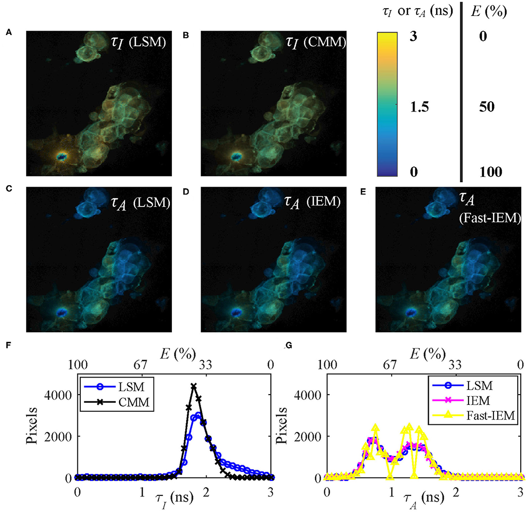
Figure 7. (A,C) τ_I and τ_A images evaluated with LSM-2, (B,D) τ_I and τ_A images evaluated with CMM and IEM, respectively. (E) τ_A image with Fast-IEM. (F) Histograms of τ_I with LSM-2 (blue) and CMM (black). (G) Histograms of τ_A with LSM-2 (blue), IEM (magenta), and Fast-IEM (yellow). The color bar represents lifetimes and the pixel brightness represents photon counts. (A–E) Can also represent FRET efficiency (E) images evaluated with the corresponding lifetime images with the color bar representing the range of E, 0 ~ 100%. (F,G) Can also be used to show the histograms of E with the upper x label.

Since the FRET efficiency E has a linear relationship with the average lifetimes as shown in Equation (5), Figures 7A–E can also be used to represent E images with the color bar in the range of 0 ~ 100%. As we mentioned in Introduction, it is straightforward to obtain E images from τ_A images, so that Figures 7C–E are proper E images. If τ_I images are misused for E, the results would be different, as shown in Figures 7A,B, leading to a different biological story.

3.2.2. Visualization of Multi-Exponential Decays With τ_A/τ_I

τ_I and τ_A can not only access the essential parameters in FRET and dynamic quenching processes but also indicate the positions where multi-exponential decays occur. As mentioned previously, a fluorescence signal can be approximated by a bi-exponential decay, so that the ratio of τ_I and τ_A can be expressed as

\begin{array}{l} \frac{τ_{A}}{τ_{I}} = \frac{{[1 + q_{1} (R - 1)]}^{2}}{1 + q_{1} (R^{2} - 1)}, & (11) \end{array}

where R = τ₁/τ₂. The distribution of τ_A/τ_I (Figure 8) shows that when R ≃ 1 or q₁ ≃ 0 or 1, τ_A/τ_I ≃ 1. With a decrease of R or an increase of q₁, τ_A/τ_I decreases. Therefore, the ranges of q₁ and R of a pixel can be determined by τ_A/τ_I.

FIGURE 8

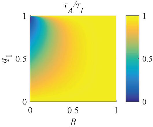
Figure 8. Distribution of τ_A/τ_I with q₁ = 0 ~ 1 and R = 0 ~ 1.

To present the multi-exponential decay visualization performance of τ_A/τ_I, the τ_I and τ_A images evaluated by LSM-2, Figures 9A,B, were used to generate the τ_A/τ_I image as shown in Figure 9C. The histograms of τ_I and τ_A and the phasor plot are shown in Figures 9D,E. Figure 9F shows the possible range of q₁ and R of the selected pixels in Figure 9C. Figures 9C,F share the same color bar. Figure 9D shows that τ_A has a broader lifetime dynamic range than τ_I, which is consistent with the theoretical lines shown in Figure 5B. The τ_A histogram shows two clusters with different peaks, whereas the τ_I histogram only indicates a single merged group, meaning that there is no way to differentiate these two clusters. It is why using τ_I to analyze samples with a strong FRET can be misleading.

FIGURE 9

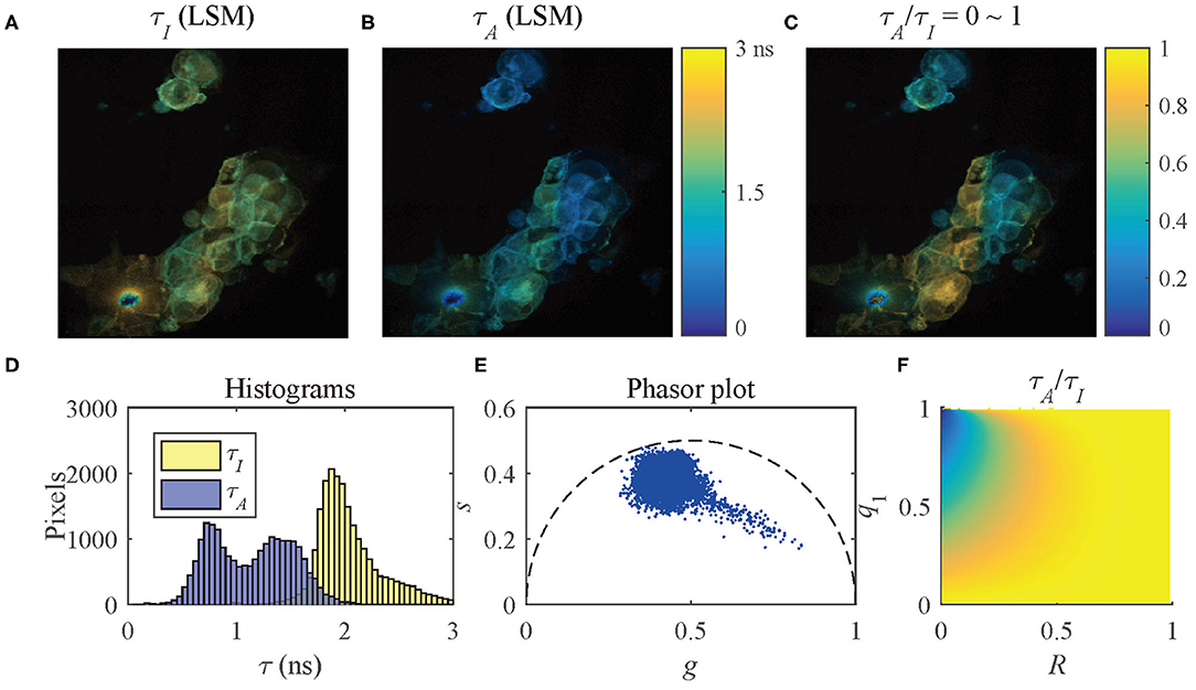
Figure 9. (A) τ_I-intensity image, (B) τ_A-intensity image evaluated by LSM-2, (C) τ_A/τ_I ratio image, (D) histograms of τ_I (yellow) and τ_A (blue), (E) phasor plot, and (F) distribution of τ_A/τ_I of the selected pixels in (C).

The results of the selected pixels within different τ_A/τ_I ranges are shown in Figure 10, τ_A/τ_I = 0.2 ~ 0.5, and Figure 11, τ_A/τ_I = 0.5 ~ 1. For the pixels with τ_A/τ_I = 0.2 ~ 0.5, the histograms clearly show that τ_A is much smaller than τ_I, which means the difference between τ₁ and τ₂ is significant. Figure 10F shows that the ranges of q₁ and R are approximately 0.5 ~ 1 and 0 ~ 0.2, respectively. For the pixels with τ_A/τ_I = 0.5 ~ 1, τ_A is closer to τ_I, meaning the pixels have decays close to mono-exponential. Separating the average lifetime images with τ_A/τ_I is easier than phasor plots because τ_A/τ_I is one dimensional and phasors are two dimensional. Furthermore, τ_A/τ_I can show the q₁ and R ranges more intuitively than phasor plots. τ_A/τ_I can be a useful tool to visualize the properties of the fluorescence decays within a lifetime image.

FIGURE 10

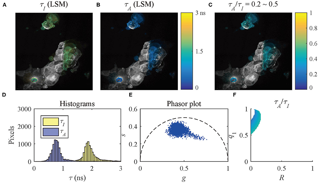
Figure 10. (A) τ_I-intensity image, (B) τ_A-intensity image evaluated by LSM-2, (C) τ_A/τ_I ratio image, (D) histograms of τ_I (yellow) and τ_A (blue), (E) phasor plot, and (F) distribution of τ_A/τ_I of the selected pixels in (C) with τ_A/τ_I = 0.2 ~ 0.5.

FIGURE 11

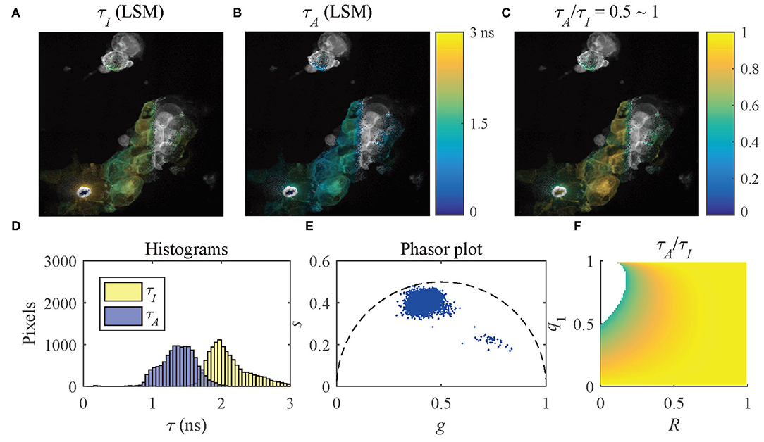
Figure 11. (A) τ_I-intensity image, (B) τ_A-intensity image evaluated by LSM-2, (C) τ_A/τ_I ratio image, (D) histograms of τ_I (yellow) and τ_A (blue), (E) phasor plot, and (F) distribution of τ_A/τ_I of the selected pixels in (C) with τ_A/τ_I = 0.5 ~ 1.

4. Discussion

In realistic samples, fluorescence signals always follow multi-exponential decay models. However, extracting lifetime components with a traditional fitting method is a time-consuming process. For some applications that require calculating FRET efficiency and accessing dynamic quenching behaviors, average lifetimes are satisfactory. Model-free lifetime determination algorithms can be used to evaluate average lifetimes directly, for instance, CMM and Phasor for intensity-weighted average lifetimes τ_I and IEM for amplitude-weighted average lifetimes τ_A. Discussions of the influence of the model mismatch between the real signal and the model-based LDAs on τ_I and τ_A estimations suggest that a bi-exponential model can well-approximate a signal following a multiple-exponential model. The results of the Monte-Carlo simulations suggest that VPM and LSM based on a bi-exponential model can be used for applications requiring high accuracy. The constrained TRR and LM algorithms with proper initial conditions are supported for LSM to guarantee accuracy. In contrast, CMM and IEM are recommended for applications requiring high estimation speeds. We also explained why τ_I models can be misleading, and τ_I and τ_A models should be considered. Experimental data were used to compare the performances of LSM-2, CMM, and IEM for evaluating τ_I and τ_A images. Similar τ_I and τ_A images were generated, whereas CMM and IEM are much faster than LSM-2. The data were further analyzed with τ_A/τ_I, which is capable of indicating the possible ranges of the amplitude proportion of the short lifetime and the ratio of the short and long lifetimes. We believe τ_A/τ_I is a useful and intuitive tool for visualizing multi-exponential decays in a lifetime image.

Data Availability Statement

FLIM image raw data and the instrument response are available at https://doi.org/10.15129/062e9e11-9d7f-49e5-a332-2b10d695bdcd.

Author Contributions

YL conducted theoretical and experimental analysis and developed analysis tools. MS and MC conceived FRET experiments and prepared samples. SN and YC contributed to FRET-FLIM experiments. JT contributed to tool developments. DL initiated the research concept and supervised the project. All authors wrote and revised the paper.

Funding

We would like to acknowledge support from Medical Research Scotland, China Scholarship Council, and Engineering and Physical Sciences Research Council (EP/M506643/1).

Conflict of Interest

The authors declare that the research was conducted in the absence of any commercial or financial relationships that could be construed as a potential conflict of interest.

References

1. Lakowicz JR. Principles of Fluorescence Spectroscopy. New York, NY: Springer (2006). doi: 10.1007/978-0-387-46312-4

ORIGINAL RESEARCH article

Investigations on Average Fluorescence Lifetimes for Visualizing Multi-Exponential Decays

1. Introduction

2. Theory

3. Results

3.1. Simulations

3.1.1. Case A: Model Mismatch

3.1.2. Case B: Performances of Average Lifetime Estimations

3.2. Experimental Results

3.2.1. Average Lifetime Images With LSM, CMM, and IEM

3.2.2. Visualization of Multi-Exponential Decays With τA/τI

4. Discussion

Data Availability Statement

Author Contributions

Funding

Conflict of Interest

References

Appendix

This article is part of the Research Topic

People also looked at

3.2.2. Visualization of Multi-Exponential Decays With τ_A/τ_I