Structured Light: Ideas and Concepts
 Oleg V. Angelsky1,2
  Aleksandr Y. Bekshaev3
  Steen G. Hanson4*
  Claudia Yu Zenkova1,2
  Igor I. Mokhun2
  Jun Zheng1
- 1Research Institute of Zhejiang University—Taizhou, Taizhou, China
- 2Chernivtsi National University, Chernivtsi, Ukraine
- 3Physics Research Institute, Odessa I.I. Mechnikov National University, Odessa, Ukraine
- 4DTU Fotonik, Department of Photonics Engineering, Roskilde, Denmark
The paper briefly presents some essential concepts and features of light fields with strong spatial inhomogeneity of amplitude, phase, polarization, and other parameters. It contains a characterization of optical vortices, speckle fields, polarization singularities. A special attention is paid to the field dynamical characteristics (energy, momentum, angular momentum, and their derivatives), which are considered not only as mechanical attributes of the field but also as its meaningful and application-oriented descriptive parameters. Peculiar features of the light dynamical characteristics in inhomogeneous and dispersive media are discussed. The dynamical properties of paraxial beams and evanescent waves (including surface plasmon–polaritons) are analyzed in more detail; in particular, a general treatment of the extraordinary spin and momentum, orthogonal to the main propagation direction, is outlined. Applications of structured light fields for optical manipulation, metrology, probing, and data processing are described.
Introduction
Despite the intensive development of the concepts and instruments, for a long time, the optical science operated with a rather limited set of the traditional optical field models. If one inspects the contents of most comprehensive manuals (e.g., the fundamental textbook by M. Born and E. Wolf [1]), he finds plane waves, divergent, and convergent spherical waves (most frequently, in conjunction with the geometric optics and the theory of optical image), some special examples of multipole radiation or scattering, and, as rare curiosities, several examples of complicated field patterns near the lens focus. However, the general impression holds that the optics deals—almost exclusively—with plane waves, rays, point sources, and smooth wavefronts. And this impression was not elusive because the traditional concepts and instruments were fairly adequate for the majority of light-related problems and optical devices.
The situation has changed during the last two or three decades when the ideas of “structured light, tailored light, shaped light, sculpted light” [2–6] have occupied prominent positions in optical research. With the rapid development of optical technologies, such as optical manipulation, data processing, optically driven micromachines, selective micro-influences, optical sorting, delivering, etc., the necessity in formation and study of the optical fields with expressive spatial inhomogeneities of the amplitude, phase, polarization, and other parameters, has become evident. A number of new seemingly abstract ideas and concepts (e.g., singularities of the phase, polarization and energy flow; notions of superoscillation and supermomentum; light topology, optical helicity and chirality, spin–orbit interaction, quantum weak measurements) have not only revolutionized the traditional optics but also become efficient instruments for technical applications. Moreover, the methods and concepts, born in connection with structured light, find further productive applications in other branches of physics, including acoustics, electron optics, etc. Now, it is clear that the idealized situations of classical optics with well-defined and smooth rays, wavefronts, etc., are rather exclusions, whereas the optical fields with strong inhomogeneities are ubiquitous and stimulate a deeper penetration into the nature of light and the optical-wave physics.
In this context, the term “structured light” is rather general and unites all optical fields where the spatial inhomogeneity of any parameter of the field is important and cannot be neglected. Of course, the variety of such situations is really boundless, and in this review, we forcedly restrict ourselves to some selected aspects and principles closely linked to our research interests. The paper starts with a short description of light as the vector electromagnetic wave and introduction of the field vectors and polarization parameters (Principles of the Structured Light Description: Paraxial Model section). Next, selected sorts of structured light fields are briefly characterized in the Sorts of Structured Light section. In particular, it follows from this overview that the traditional light-field characteristics (distributions of amplitude, phase, polarization) are not sufficient in case of fields with highly developed structures. The Dynamical Characteristics of Structured Optical Fields section is devoted to the presentation of the main dynamical characteristics of light fields (energy, momentum, angular momentum, and their derivatives), which, in addition to their value for understanding the field properties and their possible applications, may be suitable for adequate characterization of structured light. In many modern applications, the special features of the evanescent and surface light waves are intensively exploited; these are considered in the Evanescent Waves: Extraordinary Spin and Momentum section and the Surface Plasmon–Polaritons section in detail. The selected applications of the structured light, which are related with the optical manipulation, information, and telecommunication techniques and with the optical super-resolution problems, are briefly outlined in the Applications of Structured Light section. The review summary and possible lines for further development are presented in the Conclusion section.
Principles of the Structured Light Description: Paraxial Model
As was specified above, the term “structured light” embraces all light fields, which cannot be characterized by idealized models of ray optics or plane waves [2–6]. Any light structure is associated with inhomogeneities in the spatial distributions of main field parameters: amplitude, phase, polarization, etc. In general, this set of features must include the spectral characteristics, but in this review, we restrict ourselves to the case of monochromatic fields whose temporal dependence can be expressed by the complex exponential exp (−i ω t) where ω is the light frequency, and instantaneous electric and magnetic fields are determined as Re[E (R) exp (−i ω t)], Re[H (R) exp (−i ω t)]. Such fields are exhaustively characterized by the time-invariant complex electric E(R) and magnetic H(R) vectors, where R = (x, y, z)T is the vector of spatial coordinates, and the superscript “T” denotes matrix transposition. Considering only the light fields in regions free from charges and currents, the field vectors satisfy the Maxwell Equations [7]:
where k = ω/c, c is the speed of light in vacuum, ε and μ are the permittivity and permeability of the medium, respectively, and the Gaussian system of units is used.
In many cases, the physically selected longitudinal direction can be recognized, along which the field shows a certain standard behavior, while the structured-light features are associated with the orthogonal transverse direction. In such situations, the paraxial field (beam) model is appropriate where the longitudinal spatial coordinate z is qualitatively different from the transverse ones r = (x, y)T. Then, if the beam propagates in a homogeneous medium with the refractive index , its field can be expressed as a superposition of orthogonally polarized components characterized by the slowly varying (in the wavelength scale) complex amplitudes uσ(r, z) obeying the Equations [8, 9]:
Here, ∇⊥ = ex(∂/∂x) + ey(∂/∂y) is the transverse gradient, whereas σ = ±1 for the basis of circular polarizations or σ = x, y for the basis of linear polarizations, which are equally admissible in the paraxial approximation.
The total vector complex amplitude can be defined as:
where is the transverse unit vector (generally, r-dependent), ex, ey are the unit vectors of the transverse coordinates, and
form the paraxial helicity basis. In terms of the complex amplitude u, paraxial expressions for the electric and magnetic field strengths read [9, 10]:
The main (first) terms of Equations (5) and (6) describe the transverse field components, whereas the longitudinal components (second terms) are of the relative order γ = (kb)−1 in magnitude, with b being the characteristic transverse scale of the distribution u(r, z). The quantity γ is the small parameter of the paraxial approximation; Equation (2) follows from the Maxwell equations (1) after the substitution of relations (5) and (6). The longitudinal characteristic scale of a paraxial beam (usually called “Rayleigh length”) [8, 11] also exists and is equal to .
Sorts of Structured Light
Optical Vortices
An optical vortex (OV) is a typical singular structure that may occur in paraxial beams [8, 9, 12]. OV is the scalar singularity, which can exist independently of the beam polarization. In a circular OV, the scalar complex amplitude (2) is characterized by the “helical phase factor”
where ϕ = arctan(y/x), and r are the polar coordinates in the beam cross section. According to Equation (7), the field phase does not return to its initial value on a round-trip near the axis but experiences an increment of 2mπ, which corresponds to the helical wavefront shape (screw wavefront dislocation) (see Figure 1A); this means that the phase is indeterminate (singular) in the point (x = 0, y = 0). These properties are compatible with the field definiteness only if l is an integer number called “topological charge,” and the field amplitude possesses an isolated zero point (the OV core) at r = 0, so that the intensity distribution forms a bright ring (Figure 1B). Local directions of the energy flows are normal to the wavefront, and due to its helical shape, each wavefront normal possesses a certain azimuthal component; altogether, these azimuthal components form a closed loop in the transverse cross section (Figure 1A). This makes the energy propagate along complicated spiral lines (Figure 1B) rather than along the longitudinal rays as is typical for usual optical fields. The transverse components of the energy flow are responsible for the transverse energy circulation, which is a characteristic feature of the OV field and a source of the mechanical angular momentum (AM), namely, orbital AM (OAM) carried by the OV.
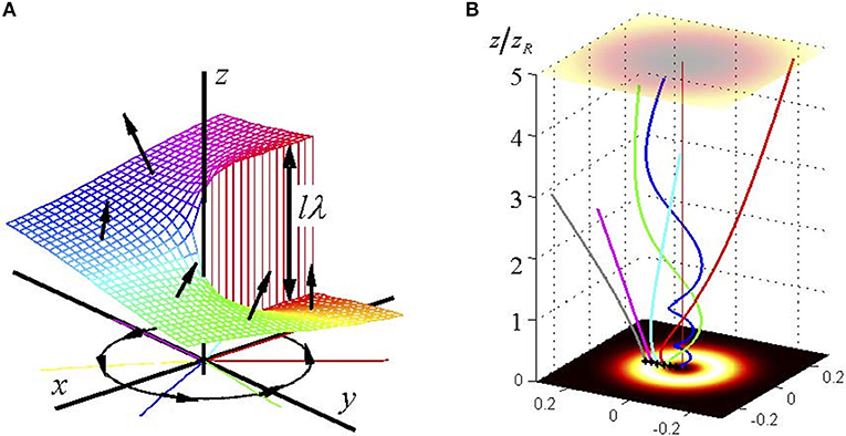
Figure 1. (A) Wavefront of an optical vortex (OV) beam near the OV core. Normals to the screw-like surface are inclined with respect to the longitudinal direction; their azimuthal components form a close-loop circulation in the beam cross section. (B) 3D lines of the energy propagation in a circular OV beam for different distances from the beam axis in the waist plane z = 0.
The circularly symmetric pattern depicted in Figure 1 shows an ideal configuration characteristic for circular OV beams (Laguerre–Gaussian, Bessel, Kummer beams, etc. [8, 11, 13–15]). In many real situations, this ideal pattern is distorted; moreover, a minor symmetry-breaking perturbation destroys a multicharged OV (with |l| > 1) into a set of |l| separate single-charged ones [8, 11]. In the nearest vicinity of the core of such a perturbed OV situated in the point x = xV, y = yV, the complex amplitude distribution can be represented as:
where βx and βy are complex parameters determining the OV morphology [8, 16, 17]. In contrast to the circular OV (7), this structure is asymmetric (“anisotropic OV”): the equal-amplitude lines are ellipses, the rate of the phase change upon the near-OV circulation is non-uniform. Under external influences (e.g., the beam propagation through inhomogeneous medium), parameters of Equation (8) βx, βy, xV, yV, may change, but the singularity “per se” with all its qualitative attributes (isolated amplitude zero, screw wavefront dislocation, transverse energy circulation) is of the topological nature and, therefore, stable against perturbations. For this reason, OV beams are promising for the information transfer in noise conditions, e.g., through the turbulent atmosphere [18] (see also the Structured Light in Telecommunication and High-Resolution Techniques section below). The intriguing dynamical properties of the OV fields [8, 9, 11, 19–21] are especially attractive for optical manipulation techniques, to be discussed in the Applications of Structured Light section.
Stochastic Structured Light: Speckle Fields
Maybe, the first bright example of spatially structured light is the spatially inhomogeneous intensity distribution formed due to scattering of coherent laser radiation by a transparent surface with stochastically inhomogeneous relief (frosted glass). This field, generated through interference of statistically independent coherent light beams has been termed “speckle field.” It represents a complicated pattern with bright and dark spots of different sizes, shapes, and localizations.
A speckle field is characterized by stochastic temporal and spatial distributions of the field parameters: amplitude, phase, and, generally, polarization. In such fields, interference of multiple differently directed waves leads to the formation of isolated points of zero amplitude with indeterminate phase (OV, see the Optical Vortices section), as well as other field singularities. However, the consistent average field characteristics can be introduced.
Here, we consider a paraxial speckle field characterized by the stochastic complex amplitude
[see Equations (2), (3)], where the function φ(x, y) describes the field phase distribution. As is well known [22], the average speckle size in the far-field zone is comparable to the correlation length. The same value determines the average distance between adjacent OVs [23]. In other words, each speckle has its own OV (essentially, only generic OVs with topological charges ±1 can exist in stochastic fields). At the same time, the concept of an individual speckle, its boundaries and size in terms of the field amplitude |u(x, y)|, is very ambiguous. Indeed, any numerical characteristic of the speckles' sizes and, after all, their number depends on the intensity level (generally, very conditional) [24], which defines the individual speckle's borders. Moreover, if zero is taken as such a level, then we will have some “table” of cores of the speckle-field OVs instead of a speckle picture.
That is why we introduce another definition of speckle, based on the following reasons:
1. The stochastic field structure manifests itself not only in intensity but also in the phase φ(x, y).
2. Nodal phase points (OV cores) are simultaneously absolute intensity minima and, therefore, are the nodal intensity points.
As is well known [25, 26], the condition for the field zeros can be written in the form:
Solutions of the first equation (lines Re = 0 in Figure 2) define equiphase lines along which the phase φ(x, y) equals ±π/2. The second equation defines a system of lines Im = 0 along which the phase is zero or π. Crossing points of such lines gives the positions of the field OVs xV, yV [see Equation (8)].
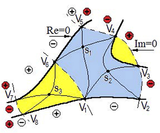
Figure 2. The field fragment with three phase speckles [27]. The areas of the adjacent phase speckles are depicted by yellow and blue. The pluses and minuses in the circles correspond to the signs of Re u (x, y) (white circles) and Im u (x, y) (red circles) in this field area.
Now consider the spatial structural element of the field bounded by the Re = 0, Im = 0 lines (from now on, we will call these lines “phase threshold lines,” or PT-lines), which, together, form a once-folded closed line. Let us call this field element “phase speckle”; in Figure 2, such areas are colored in yellow and blue, in order to distinguish the adjacent phase speckles. Naturally, locations of the PT-lines change if the field phase is changed by a constant phase factor Δ, φ(x, y) → φ(x, y) + Δ. However, the nodal points of the amplitude and stationary points of the phase are the fixed elements of the phase speckle. Fields with different Δ are physically equivalent, but depending on Δ, the PT-lines oscillate in space approaching the saddle points (points S in Figure 2) and diverging away from them. Nevertheless, for any Δ, the field phase within the phase speckle can be considered practically constant (within ±π/2, the Rayleigh criterion) [28]. It is this fact that served as basis for the phase-speckle concept. Taking into account the signs in the regions bounded by the PT-lines in Figure 2, it is easy to conclude that the neighboring OVs directly connected by the PT-lines have opposite topological charges. This fact underlies the “sign principle” [29], establishing a connection between all OVs of the stochastic field.
Note that in most cases, at least one saddle point S is located inside the phase-speckle (exceptions may occur for phase speckles enclosed by only two lines Re = 0 and Im = 0, which intersect twice, with two OVs at their crossing points; see in Figure 2 the yellow speckle between V3 and V4). In Figure 2, such saddle points belong to the thin solid equiphase lines connecting the neighboring OVs of the same sign. On these lines, the field phase φ is averaged over the phase speckle. It can be seen from Figure 2 that the position of such a line in the OV vicinity can be established with a high degree of probability, if the PT-lines and the OV topological charge are known. From this fact, the general statement follows: if we know the positions of the field OVs, their topological charges, and the PT-lines, then, we can determine the phase at any point in the field with a sufficient reliability. In this sense, a network consisting of the OVs and PT-lines (or any other four equiphase lines with a phase increment of π/2) can be considered a specific phase skeleton of a scalar optical field.
Common nodal points of the phase and intensity—the field OVs—suggest a closer relationship between the phase and intensity distributions. For the intensity field, a network of singular points, extrema, and gradient streamlines can be constructed. As can be seen from Figure 3, the intensity-gradient streamlines, starting at the saddle points, go toward the intensity maxima or the absolute minima (OV cores). Alternatively, the gradient streamlines may tend to go toward supplementary intensity minima. However, the number of such minima is 14–16 times less than the number of OVs [27], so this alternative can be neglected.
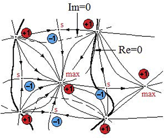
Figure 3. Nets of the special points of intensity and singular points of phase formed by the intensity-gradient streamlines and by the phase threshold lines (PT-lines). Poincaré indices are indicated for the intensity maxima (max), OVs (absolute minima, red circles), and for the saddle points of intensity (S) (blue circles) [27].
Such an interpretation of the stochastic field structure leads to new phase-reconstruction algorithms based on the analysis of the intensity distribution [30–32]. Moreover, it clarifies the speckle formation mechanism. For example, consider the situation where a scattering object (e.g., ground glass) is used to introduce a pure phase modulation. Immediately behind the scattering object, modulation of the field is phase-only; therefore, the OVs are absent in the object's boundary field. The OVs emerge due to multi-beam interference in the near field where the phase modulations produce amplitude inhomogeneities. For example, such near-field speckle patterns are formed in laser-illuminated biotissues, and the correspondence between the speckle sizes and the characteristic cell-structure sizes is considered as a reason for biological effect of low-intensity laser radiation [33, 34].
When vortices are generated, their numbers grow sharply so that at the beginning of the Fresnel zone, the number of amplitude zeros (within the angular divergence of the field) reaches its resulting value, which does not change while going to infinity. Figure 4 schematically shows the development of a 3D speckle pattern. The so-called shadow region, where the speckle pattern is formed, is the zone of OV generation. For this reason, the evolution of OVs within the Fresnel zone differs from their evolution during the far-field propagation. The “body” of a speckle within the Fresnel zone is of a more or less “true” ellipsoidal shape.
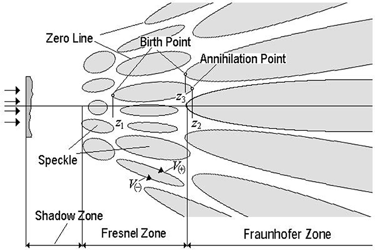
Figure 4. Schematic illustration of the speckle field evolution [27].
The speckle sizes (including the longitudinal sizes) are finite and increase as the observation plane moves toward the Fraunhofer zone. In this case, the boundary of a speckle (its cross section) can be described by single-fold curves. The lines, or trajectories, of amplitude zeros lie on the speckle boundary, containing closed single-fold curves. In Figure 4, such lines are shown as planar curves of the oval-like shapes, but actually, these can be complex three-dimensional lines with unpredictable trajectories [35]. Nevertheless, the simplified picture of Figure 4 conveys a useful illustration of the consistent analysis of OVs' generation and annihilation process.
Indeed, if the plane of analysis moves along the z-axis, one observes the birth, propagation, and annihilation of vortices. An OV is born at the point where the line of amplitude zero, winding around a speckle body, is tangent to this plane (point z1 in Figure 4). Further translation of the observation plane along the z-axis results in the appearance of two OVs, V(+) and V(–), up to the point where the zero line of amplitude is tangent to this plane again (z2). Here, the OVs annihilate. In other words, evolution of vortices within the Fresnel zone (with constant mean density of OVs) can be considered as alternating events of birth and annihilation of the OV pairs. In this view, the OV-network dynamics within the Fresnel zone radically differs from the evolution of OVs in the far field, where the lines of amplitude zeros tend to infinity. With growing propagation distance z, the number of the OV birth/annihilation events decreases, and ultimately, these events do not occur anymore. The OVs generated from multi-beam interference do not annihilate in the far field, that is, the stationary (within the angular-divergence factor) speckle pattern is observed at z → ∞.
Polarization Singularities: Singular Skeleton
The situation for a vector field differs considerably from the scalar case. In contrast to the scalar field, stationary amplitude zeros are absent in the vector field. In reality, the presence of a stationary amplitude zero in a vector field presumes simultaneous zeros for all three orthogonal components in a single point. The probability of such an event is negligible. Moreover, existence (if even supposed) of this zero is doubtful, while an infinitesimal disturbance results in a shift of the components' zeros from their initial position. Thus, a stationary singularity of this kind may only be regarded from the point of view of model conditions, where the distance between the component zeros is too small to be reliably detected in the experiment. In this case, the behavior of the field in the vicinity of such a “model” singularity will be the same as in the case of a true zero of the vector field.
For vector fields (in the paraxial approximation), one can specify the following main types of stationary polarization singularities [26, 27]:
1. The s-contours (sometimes called L-lines), in 3D space s-surfaces, where field is linearly polarized; the rotation direction of a field vector is indeterminate at these contours.
2. C-points (in 3D space, C-lines) are the points (lines) of circular polarization, where the polarization ellipse degenerates into a circle, and the ellipse orientation angle becomes indeterminate, as well as the magnitude of the so-called vibration phase that determines the electrical vector direction with respect to the large axis of the ellipse. Such points may be characterized by the Poincare index, which equals to ±1/2 and characterizes the rotation of the polarization ellipses on a round trip near the C-point [26]. In the circular-polarization basis [see Equations (3), (4)], a right-polarized C-point coincides with the isolated zero (OV) of the left-polarized component, and vice versa.
There are two different principles of the s-contour formation [27]:
• when a region with any specified handedness of polarization is surrounded by an area with the opposite handedness, this outer area is, again, surrounded by a larger area with altered handedness, and so on—a hierarchy of enclosed areas is formed with alternate polarization handednesses whose boundaries are the s-contours (Figure 5A);
• s-contour of another type simply separates topologically disconnected areas of right-hand or left-hand polarizations (Figure 5B).
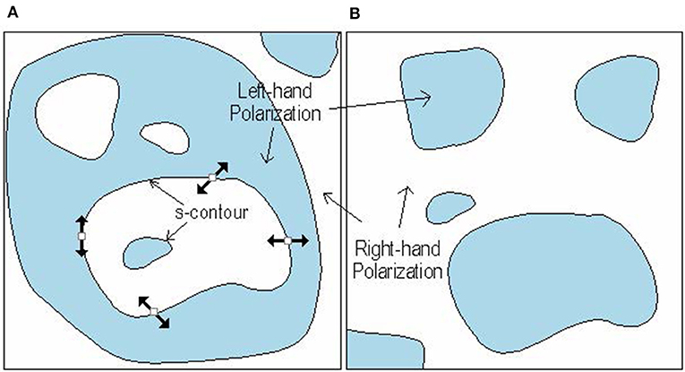
Figure 5. Different types of the s-contour structure [27]. (A) hierarchy of enclosed areas with alternating polarizations; (B) isolated areas (“islands”) of one polarization surrounded by the “sea” of the opposite polarization.
Similar to the case of scalar field, the sign principle for polarization singularities can be formulated: two adjacent C-points, which can be immediately connected by an equi-azimuth line (along which the polarization ellipses preserve their orientation), have Poincare indices of opposite signs [36, 37]. A fragment of the vector field cross-section with polarization singularities is schematically presented in Figure 6. It shows that if we know the orientation of the field vector at some point of the s-contour and the topological characteristics of the nearest C-point, then we can, with some probability, say that at a certain point between the s-contour and the C-point, the polarization ellipse possesses a certain ellipticity and orientation. In this sense, a set of polarization singularities, as in the case of a scalar field, can be considered as a skeleton that governs the field behavior at any point between the singularities.
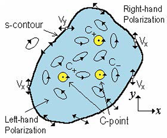
Figure 6. The field fragment with s-contour and a set of C-points. The OVs of the ux and uy components (see Equation 3) lie on the s-contour and are indicated by Vx and Vy, respectively [27].
Dynamical Characteristics of Structured Optical Fields
General Definitions
In view of the specific properties of structured light fields, the usual means for their characterization based on the intensity and phase distributions, in many cases, become insufficient. For a lot of applications, a system of the field parameters that addresses the field's physical actions more directly is desirable. To this end, the field dynamical characteristics (DCs), which include the energy and momentum of the field with some of their derivatives (AM, spin, helicity, etc.) may be more applicable [9, 10, 12, 20, 38–42].
The main DC of an optical field is its energy averaged over the period of oscillations that is distributed with the volume density [7]:
whereas the measure of the energy flow density is given by the time-averaged Poynting vector [7]:
Here, g is the constant factor, which equals g = (8π)−1 in the Gaussian system. Quantities (9) and (10) determine the local group velocity with which the energy propagates,
for guided spatially confined modes, the average group velocity can be defined as:
(from now on, 〈…〉 means integration over the spatial dimension(s) in which the field is limited so 〈w〉 denotes the integral energy of the field, and 〈S〉 is its integral energy flow).
Note that due to requirements of the special relativity, the Poynting vector also expresses the momentum density of the field. However, for the momentum in material media, two approaches have been competing for over a century [43–49]: the Abraham pA and Minkowski pM momenta are defined as:
Accordingly, the AM density of light is given by
This quantity depends on the reference point (coordinate origin). For some problems, it is more convenient to define the AM with respect to the (longitudinal) z-axis; in this case, the 3D radius-vector in Equation (14) is replaced by its transverse projection: R → r.
By using the Maxwell equations for monochromatic fields [7], the Minkowski momentum density (13) can be written as:
where
() represent the “spin” and “orbital” (canonical) [12, 50, 51] constituents of the total momentum. Note that electric we, , , and magnetic wm, , contributions are separated in Equations (9), (16), and (17) and enter these equations on an equal footing (“electric–magnetic democracy”) [20]. We emphasize that the compact form (15)–(17) of the momentum decomposition is correct even in the case of spatially inhomogeneous medium. This is a special property of the Minkowski momentum [52]. Corresponding decomposition for the Abraham momentum contains poorly interpretable “gradient terms” depending on ∇ε and ∇μ [52–55] (and this is an additional argument for the Minkowski vision, together with the recent relativistic reasoning based on the wave-packet propagation analysis) [46–49].
The immediate formal sense of the momentum decomposition (15)–(17) is that and are the sources of the spin (SAM) s and orbital (OAM) L AMs of light, j = s + L. Further, due to the relation ∫ R × (∇ × s)dV = 2 ∫ sdV, valid for any spatially confined field, the SAM density and the spin–momentum (SM) density pS can be presented in the forms:
The OAM expression follows immediately from the definition (14):
(again, expressions (18) and (19) are based on the Minkowski momentum definition, which is proven to be more appropriate for the AM of light in material media than the Abraham's one) [48, 56].
The general form of the spin density means that the SAM of the “whole” field 〈s〉 = = ∫ sdV does not depend on the reference point: the SAM is an intrinsic property of the field [9, 12]. In contrast, the OAM (19) reflects not only the details of the intrinsic spatial configuration of the field but also the position of the field “as a whole” with respect to an (arbitrary) coordinate frame. In many cases, one can introduce a “preferential” frame with the origin RC, associated with the field, in which the OAM characterizes the field “per se”; then, the intrinsic and extrinsic parts of the OAM density can be determined [9, 12, 57]:
Usually, RC characterizes the field “center of gravity” defined as [9, 12]:
The two parts of electromagnetic momentum show distinct mathematical and physical discrepancies. The orbital momentum (OM) (17) immediately enters the energy-momentum tensor [7] and appears in the general field-theory formalism from the field Lagrangian and the momentum conservation via the Noether theorem [12, 58] (that is why it is also called “canonical”). Its immediate physical meaning follows from the fact that it is proportional to the local energy flow in the field. In the same general formalism, the SM (16) appears rather formally due to the energy-momentum tensor symmetrization [59] and for a long time was considered as a “virtual” quantity [12, 50, 51] important for the theory but not meaningful practically. Owing to its solenoidal character (∇ · pS = 0), the SM does not participate in the “net” energy transport, and for spatially confined fields, the integral SM value vanishes [9, 20]:
Still, from the field-theory point of view, the spin–orbital (canonical) momentum decomposition (15)–(17) looks deficient because the separate OM and SM (as well as the SAM and OAM) are not gauge invariant [9, 20, 60]. However, in optics, at least in the considered situation of monochromatic fields, the gauge is always fixed, and the structured light theory provides bright and instructive examples where the gauge-dependent quantities are physically meaningful and useful for applications despite their theoretical “impurity.”
The very term “dynamical characteristics” means that the quantities considered in this section express such features of light that are naturally manifested in the dynamical interactions of light waves. Really, all DCs are associated with certain aspects of the mechanical action of light fields on material objects. This association can be expressed in a simple analytical form in the case of small particles whose electromagnetic properties are exhaustively characterized by the field-induced electric αeE and magnetic αmH dipole moments (“dipole particles”) [61, 62]. For example, the optical force F exerted on such a particle is determined by the sum F = Fe + Fm + Fem where:
First of all, these equations clearly demonstrate suitability of the gauge-dependent canonical decomposition (15)–(17). Equations (23) and (24) by no means testify that the mechanical forces [as well as the torques, see (Equation 26) below] are gauge dependent, despite the presence of gauge-dependent quantities pO and pS. Actually, the mechanical action originates from the immediate interaction between the external electric/magnetic fields and the field-induced charge redistributions (dipoles, quadrupoles, etc.) in the material objects. The whole pattern “per se”' is completely gauge-invariant but, under the fixed gauge conditions accepted in optics, can be usefully interpreted via the OM and SM components.
Equation (23) describes the “electric” and “magnetic” dipole forces due to the electric αe and magnetic αm polarizabilities. Their first terms are the components of the gradient force generated by the inhomogeneous energy distribution (9). The second terms express the dipole contributions of the usual light pressure and testify that the light pressure originates from the OM constituents. In contrast, the mechanical action of the SM appears only in higher dipole orders due to interference between electric and magnetic dipole scattering, when the particle possesses both electric and magnetic properties. The first summand of Equation (24) seemingly suggests that only the “combined” mechanical action supplied by the sum of SM and OM can be detected, but in many practical situations, the two constituents can be easily separated spatially or by their directions [50, 51, 61–63] (for example, see the Structured Light in Optical Tweezers and Micro-Manipulation Techniques subsection Figure 12 [64]). Equation (24) shows that the SM-induced force can expose rather paradoxical features like “pulling” small particles against the direction [41, 61], which is typical for dielectric particles with real positive αe and αm. The last term of Equation (24) contains the so-called “reactive momentum”:
which is, therefore, an additional DC able to produce a distinct mechanical action [40, 41, 50, 51, 63].
Equations (23) and (24) show that the optical absorption is not necessary for the optical dipole force: a non-zero mechanical action on a particle with real αe, αm is quite possible. This is in contrast with the spinning mechanical action exerted by fields with SAM: a dipole particle can feel the field-induced mechanical torque T = Te + Tm only if it absorbs a part of the incident radiation [50, 51],
This fact can be used, e.g., for measurement of weak light absorption [65].
In addition, to finalize the recital of DCs, we mention the electromagnetic helicity [60, 66], which is especially important for various aspects of the chiral interactions and electromagnetic duality manifestations in structured light fields:
The energy, momentum, spin, and helicity densities are independent quantities, and together with their derivatives and meaningful constituents (members of the spin–orbital decomposition, partial contributions of the separate polarization components, etc.), they form a complete set of fundamental dynamical properties of light [12].
Dynamical Characteristics of the Paraxial Fields
In the special case of paraxial beams [Equations (3)–(6)], the DCs find simple and physically transparent mathematical expressions that additionally elucidate their meanings and descriptive abilities.
In the first-order approximation in γ, the longitudinal field does not affect the energy density (9), which takes the form:
The SM (16) can be described as:
where we use the complex transverse coordinates
and a paraxial representation of the helicity (27),
with
being the coordinate-dependent Stokes parameter [1] responsible for the degree of circular polarization. Equation (29) shows the intimate relation of the SM with the structured nature of the field because it only appears in spatially inhomogeneous conditions. This intimate relation is explained by the physically transparent picture of the SM origin due to the combination of microscopic circulation cells [8, 9, 67–70]. According to Equation (29), the paraxial SM is purely transverse and of the first paraxial order in magnitude (~γ). Within the beam cross section, it is directed along the constant-helicity lines for which s3 = const; in homogeneously polarized beams, the SM has a circulatory character near each intensity extremum, and the corresponding energy flow c2pS performs no energy redistribution [9, 42].
For the OM (17), the paraxial approximation naturally gives the separate longitudinal and transverse contributions:
The first term,
describes the main (plane-wave-like) longitudinal part; its spatial distribution exactly reproduces the light energy distribution (28). In paraxial case, the beam intensity,
equally characterizes the energy or momentum distributions; moreover, different detectors measuring either w or the energy flow within a limited solid angle and sensitive either to an electric or magnetic field [9, 67, 71] are equivalent with respect to the spatial intensity distribution. Additional features of the beam's structured nature are revealed by the second (transverse) term of (33), which can be recast in the form:
where the real phases of functions uσ = |uσ|exp(iφσ) are introduced. Equations (33)–(35) show that, in contrast to the SM, the OM can be divided into partial constituents belonging to the orthogonal polarization components, and these constituents are directed along the wavefront normals of the corresponding polarization components [9, 10, 42].
Note that according to Equations (29)–(33), the “full” electromagnetic momentum (15) consists of three summands: the “orbital” terms pO∥ and pO⊥ (33) represent the longitudinal and transverse helicity-independent contributions, while the SM term pS (29) expresses the specific momentum contribution associated with the beam helicity. Likewise, the spin density (18) in paraxial beams acquires the form:
where
are the longitudinal and transverse components of the usual spin directly associated with the field helicity and vanishing in the linearly polarized or scalar fields. In contrast, the last term of Equation (36),
describes the helicity-independent spin, specific for structured light fields. It is not related to the polarization but originates from the spatial inhomogeneity of the momentum and/or energy. This spin appears due to the field vector rotation in the longitudinal plane, and its analogs were recently discovered even in acoustic fields [72]; it is usually referred to as the “transverse spin” [12, 50, 51, 73]. However, this nomenclature may be inconvenient beyond the paraxial approximation because the well-defined “longitudinal” and “transverse” directions may be absent in highly structured fields. It is tempting to call it “momentum spin,” as a reciprocal to the “spin momentum” of Equation (29), but this may be confusing, and therefore, the term “extraordinary spin” will be used. Existence of extraordinary spin and momentum with directions different from the wave propagation is a characteristic feature of structured light and is attracting much attention [74]; their specific examples and possible applications are discussed below in the Evanescent Waves: Extraordinary Spin and Momentum section, Surface Plasmon-Polaritons section and the Applications of Structured Light section.
The latter Equation (39) discloses an interesting relation between the sE and the vorticity [9, 20] (curl) of the OM. Remarkably, in the paraxial approximation, keeping only the first-order terms in γ, this relation can be treated wider as a link between the spin and the total momentum (15) [75]:
In this form, the reciprocity between the extraordinary spin (39) and the SM (29) becomes especially remarkable: sE is determined by the curl of momentum just like the SM (18), (29) is determined by the curl of the spin.
In view of Equations (29) and (33)–(39), one can derive another useful spin–momentum relation:
In particular, it means that in fields with pure right (u− ≡ 0) or left (u+ ≡ 0) circular polarization (eigenstates with well-defined helicity [12]), the spin and momentum are mutually colinear:
The OAM density with respect to the z-axis per unit z-length of the beam reads:
Calculations with Equation (35) result in:
[cf. Equation (7)]. For circular homogeneously polarized OV beams [u− (r) ∝u+ (r) depend only on r, φ = lϕ, see Equation (7), Optical Vortices section], Equations (28) and (44) entail that:
In conclusion of this section, we present the paraxial expression of the reactive momentum (25):
where s1 and s2 are the spatially variable Stokes parameters
and ξ, η are the complex coordinates (30). Equation (46) reveals the characteristic symmetry properties of the reactive-momentum force described by the last term of Equation (24). In particular, in case of linear polarization, this force resembles the gradient force [76], however, with opposite signs along the orthogonal directions. This force was studied numerically [40] and discussed based on intuitive arguments [42] as a “polarization-dependent dipole force.”
Finally, we underline that the paraxial expressions presented in the current section are valid if γ = (kb)−1 ≪ 1, i.e., the characteristic size of the field inhomogeneity b must be much larger than the wavelength λ = 2π/k. This condition expresses the approximate character of the paraxial beam model. However, it may be qualitatively valid when b equals several wavelengths, e.g., for strongly focused beams [73, 77, 78] and provide a reasonable numerical description of the spin-induced phenomena in the focused fields with moderate numerical aperture [1] (NA ~ 0.1) [10, 79].
Dynamical Characteristics of Optical Fields in Dispersive Media
In most cases, the structured light fields are closely coupled with the structured matter, and any electromagnetic medium shows the more or less strong dispersion (frequency dependence of the main electric and magnetic parameters) and absorption. Sometimes, while the light frequency is far from the absorption bands of the medium, this frequency dependence can be discarded with no or very small loss of accuracy, and the description of the DCs in such situations was outlined above. However, in most interesting cases, the dispersion-free approach is insufficient, e.g., in application to surface light waves where strong dispersion and spatial inhomogeneity are inevitable.
In order to develop a consistent means for the DC description in dispersive media, the mathematical and physical attributes of the DCs were carefully revisited [52, 56, 58, 80–82]. First, in the frame of phenomenological Lagrangian formalism, via formulation of the energy-momentum tensor in dispersive media and using the Noether theorem in pursuit of the conserved quantities, the dispersion corrections for the field momentum and AM were derived [56, 58]. Based on these results, it was shown that the influence of dispersion can be accounted for by means of introducing the dispersion-modified permittivity and permeability into the regular DC expressions (9), (16)–(18), and (27) [52, 81, 82].
Remarkably, the general model of the dispersion corrections continues along the way paved more than a century ago by the well-known Brillouin formula for the energy [83]:
where “~” denotes dispersion-modified quantities, and ε and μ are assumed to be real. This expression differs from the non-dispersive version (9) by the replacements , . Note that in dispersive media, ε and μ can be negative, and then Equation (9) may cause negative-energy inconsistencies, while and are always positive.
The energy flow density S is still described by the kinetic Abraham momentum [52, 81] (10), and the group velocity is determined by Equations (11) and (12) with dispersion-modified energy density, e.g., . However, expressions for the OM, SM, SAM, and OAM [Equations (16)–(19)] in dispersive media acquire the forms [52, 81, 82]:
Note that the dispersion corrections are applied not to the Poynting momentum [Equation (13) or (15)] but to the constituents (16) and (17) of its spin–orbital (canonical) decomposition. This means that, for the field in a dispersive medium, it is the SM and OM that are fundamental rather than the “full” momentum, no matter whether it is in its Abraham (13) or Minkowski (15) form. In this pattern, the full electromagnetic momentum appears as a derivative quantity formed as a sum of the dispersion-modified SM and OM.
The exclusive role played by the SM and OM for the DC description under dispersive conditions discloses additional important and unexpected features of the spin–orbital decomposition of the electromagnetic momentum (15)–(17). Noteworthy, in case of negligible dispersion, the results (49)–(51) reduce to the expressions following from the Minkowski paradigm, thus, supplying its additional support.
Also, the general approach [56, 58] leads to the dispersion-modified helicity expression [80] [cf. Equation (27)]
Note that the dispersion-modified expressions for the electromagnetic DC are not necessary for explanation of their mechanical action on suspended particles but are rather important for understanding the dynamical properties of the field as a whole. In view of the mechanical actions, any material probe immersed in the medium feels the “pure” electromagnetic field and feels the field-induced medium motions but with different sensitivities. This means, for example, that the “total” dispersion-modified momenta (49) and (51) and spin (50) (or their electric and magnetic parts separately) cannot be substituted into Equations (23), (24), and (26) for the field-induced force or torque. The mechanical action of the field “per se” is determined by the “pure” field parts of the spin or momentum discussed in the General Definitions subsection, whereas the mechanical action of the medium motions (if it exists) is determined by some completely different non-electromagnetic mechanisms.
In this context, the last element of the DC set discussed in this paper, the reactive momentum (25), shows no known physical manifestations related to the dispersion; that is why the search of its dispersion-modified expression currently looks meaningless [39, 84].
Evanescent Waves: Extraordinary Spin and Momentum
Another characteristic and very important example of structured light fields is supplied by evanescent waves (EW) [1, 85]. Such waves show oscillatory and propagating behavior along a certain surface but exponentially decay in the off-surface direction. They appear in the optically denser medium in case of total internal reflection [54, 63, 84–86], outside a dielectric waveguide [85, 86], near curved reflecting surfaces (whispering gallery modes), near a metal–dielectric interface [surface plasmon–polariton (SPP)] [39, 52, 81, 82, 85–87], etc.
Let us consider the EW propagating parallel to the (y, z)-plane (see Figures 7A,C). It can be regarded as a plane wave rotated through a complex angle. Let this “initial” plane wave propagated along axis z and the field vectors be presented as:
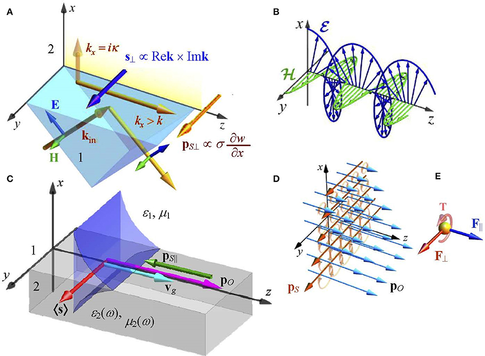
Figure 7. Evanescent waves and their characteristics (adapted from [12, 39], © 2019 with permission from Elsevier). (A) Evanescent waves (EW) (55), (56) generated by the total internal reflection of a plane wave with the wavevector kin; arrows show the wavevectors, transverse extraordinary SAM density (64) and the SM (65); (B) z-distribution of the instantaneous electric and magnetic fields and for the simplest linear x-polarization [TM mode with m = 0, τ = 1, Equations (55), (56)]. (C) Double-EW structure of the surface plasmon–polariton (SPP) propagating along the interface between media 1 (dielectric) and 2 (metal); the cyan, magenta, red, and green arrows show the group velocity, orbital momentum (OM), spin and the volume part of the SM, correspondingly. (D) Cross section of the EW with non-zero σ (54): blue arrows show the OM lines pO (with exponential decay in the vertical x-direction), closed loops, squeezing with growing x, symbolize the elliptic polarization whose inhomogeneity generates the transverse SM pS. (E) Main mechanical actions: longitudinal light-pressure force F|| caused by the OM (66), transverse force F⊥ due to the extraordinary SM (65) and the longitudinal torque due to the helicity-dependent spin sz (63) [possible vertical torque produced by electric or magnetic components of Equation (62) and the transverse torque due to the extraordinary spin (64) are not shown].
Here, A0 is a complex constant related with the wave amplitude, and the complex parameter m determines the state of polarization. It can also be described by the normalized Stokes parameters:
Note that τ2 + χ2 + σ2 = 1, and τ determines the degree of linear polarization in the (x, y)-directions, χ—in directions ±45°, and σ determines the light helicity (degree of circular polarization). Actually, τ, χ and σ correspond to normalized quantities s1, s2, and s3 introduced for paraxial beams in Equations (32) and (47); now σ is not obligatory equal to ±1 but can take any value within the interval (−1, 1), as well as can τ and χ. The EW propagating along axis z is obtained from the plane wave (53) via the rotation by a complex angle iα, which is described by the rotation matrix:
and leads to the results:
where kz = nk cosh α > nk and κ = nk sinh α, and A = A0/cosh α. Formally, Equations (55) and (56) describe a plane wave with the complex wavevector:
whose real and imaginary parts are orthogonal, Im k⊥ Re k (see Figure 7A).
For example, an EW of the forms (55) and (56) is formed in the half-space x > 0 if the plane x = 0 separates it from the homogeneous medium with parameters ε1 and μ1 (Figure 7A) so that , and the plane wave (53) approaches the interface from x < 0 at an angle θ1; then,
In the non-dispersive situation, immediate substitution of Equations (55) and (56) into Equations (9) and (13) yields expressions for the energy and momentum densities:
where the third relation (54) is used. The electric and magnetic parts of the energy density can be written as:
According to Equation (18), the spin density of the EW is:
Note that the electric and magnetic constituents of the z-component are equal, and the x-oriented components exactly compensate each other (however, their mechanical action can be revealed due to selective sensitivity (26) of material particles [50, 88–90]). The total spin se + sm completely belongs to the (yz)-plane:
Its z-component sz emerges due to elliptical polarization of the EW and is analogous to the helicity-dependent spin (36)–(38), while the y-components describe extraordinary polarization-independent spin [analog of sE (39), (40)]. At first glance, the existence of the transverse spin contradicts the system symmetry for which the plane (xz) is the mirror-symmetry plane, but the fact is that the spin is an axial vector, which does not change sign upon reflection. This extraordinary spin is a characteristic feature of EWs (see Figures 7A,C), and it is the EW where its existence was first discovered [50, 53]. It originates from the field vector rotation in the longitudinal plane clearly seen in Figure 7B. Remarkably, the handedness of this rotation [and, therefore, the transverse spin direction characterized by the 1st summand of Equation (63)] is coupled with the direction of the EW propagation, which can be expressed as [cf. Equation (57)]:
The first part of the above relation [12] immediately connects the spin with the directions of propagation Re k and of the EW attenuation Im k. The same property (however, in a less evident form) is formulated by the second part of Equation (64) [75], which represents the “evanescent” version of Equation (40) and follows from Equations (59), (60), and (63). The spin–momentum coupling described by the above equations is widely used in applications for unidirectional excitation and controllable switching of surface waves [77, 91–95]. In more detail, these applications are considered in the Optical Switching and Signal Processing: Applications of the EW and SPP Properties subsection.
The components of the SM are determined through Equations (62) and (63) and the last Equation (18), giving:
The main feature of Equation (65) is the transverse direction of the “extraordinary” momentum pS⊥ ∝ ey (see Figures 7A,D), which can produce the extraordinary y-directed force (Figure 7E) [50, 63, 96] (note that the mechanical action of an EW can be calculated using the classical Mie scattering theory adapted to plane-wave fields (53) rotated through a complex angle, see Equations (55), (56) [96]). This transverse force, again, seemingly contradicts the system symmetry with respect to the (xz)-plane. However, it emerges due to the non-zero helicity σ, which destroys the mentioned symmetry.
The OM constituents appear to be proportional to the corresponding energy-density constituents [cf. Equation (34)]:
Quite expectedly, the OM is completely longitudinal (along the direction of the wave propagation). Interestingly, the z-oriented SM and OM are directed oppositely (see Figure 7C) and satisfy the relations:
where pz is the longitudinal component of the Poynting–Minkowski momentum (15). Since , Equation (67) means that an EW is able (locally) to carry the “supermomentum” [12, 53] that exceeds the momentum of a plane wave with the same energy (higher than nk per photon) [97, 98]. Also, the force exerted on a particle by the EW can be higher than the force from the plane wave with the same local energy density [50].
The group velocity of the EW can be determined by either of Equations (11) or (12) because of the similarity in spatial distributions of the energy (59) and the Poynting momentum (60), which entails the same energy flow distribution S. Taking the Abraham counterpart of expression (60), one easily obtains:
This result shows that the energy propagates with subluminal velocity directed in agreement with the wave propagation (in more complex strongly dispersive and SPP-supporting systems, EWs with zero or negative group velocities may also exist) [39, 95, 99, 100].
Finally, the helicity (27) and the reactive momentum (25) of the EW described by Equations (55) and (56) can be determined as:
As is seen, the reactive momentum does not possess a longitudinal z-component. Like in Equation (46), the mechanical action of the x-component of the second Equation (69) is similar to the gradient force action (see Equation 24), and even more, this x-component is colinear with the gradient force. However, the reactive momentum resembles the SM by the existence of an “extraordinary” transverse y-component proportional to the parameter χ just like the y-component of the SM (65), which is proportional to the helicity σ. Together with Equation (24), this means that the transverse force may emerge in the EW not only due to ellipticity (polarization-dependent SM) but also due to the linear 45°-polarization. The corresponding transverse mechanical action of the extraordinary SM and reactive momentum was convincingly demonstrated in experiments with the EW formed above the total-reflection glass–air interface [63].
Surface Plasmon–Polaritons
An interesting and meaningful case of EW can be realized at interfaces between conductive and dielectric media (Figure 7C). In the optical-frequency range, many natural [86, 87, 101] (and artificial [102, 103]) conductive materials possess negative real part of the permittivity and a relatively small imaginary part responsible for the light dissipation. In such conditions, the double-evanescent field, attached to the interface and exponentially decaying on both sides, can propagate rather long distances without perceptible damping (up to the 0.1-mm scale [86], which is practical infinity in nano-optics). Such waves are formed by the coupled excitation of the electromagnetic field and plasmon oscillations in metal, and are called surface plasmon–polaritons (SPPs) [39, 52, 81, 82, 85–87].
Figure 7C represents a model structure supporting the SPP propagation: medium 1 (dielectric) with permittivity ε1 and permeability μ1 occupy the half-space x > 0, while at x < 0, the metallic medium 2 is situated. The characteristic distinction of SPPs from other EWs considered in the previous section is the strong dispersion of the medium 2 electromagnetic parameters ε2(ω), μ2(ω). In the lossless approximation Im(ε2(ω), μ2(ω)) = 0, the electric and magnetic fields of the TM surface mode read [39, 52, 81, 82]:
Here, As is the coordinate-independent normalization constant [the subscript distinguishes it from the constant A in Equations (53)–(59)]:
the propagation constant ks is the SPP counterpart of kz in Equations (55) and (56). For existence of the TM mode, ε1 and ε2 must have opposite signs. For certainty, we accept ε1 > 0, μ1 > 0, and then one of the two sets of conditions must hold that enable the SPP propagation: either ε2 < −ε1, μ2 > −ε1μ1/|ε2| or −ε1 < ε2 < 0, μ2 < −ε1μ1/|ε2|.
Owing to the spatial confinement, the SPP field can be characterized by the integral values of its DC [cf. Equation (12)], and as the considered SPP field (70), (71) is homogeneous in both z- and y-directions, only the integration over x is meaningful. So, in Equations (74)–(80) and Figure 8 below, < …> denotes surface densities per unit area of the (yz)-plane. All the DCs essentially depend on frequency in compliance with the functions ε2(ω), μ2(ω) and Equation (72); the dependence can be rather intricate for various natural media and metamaterials [101–103]. The illustrations are given in Figure 8 for the simplest case of the standard plasma (Drude) model [81, 86] with the plasma frequency ωp:
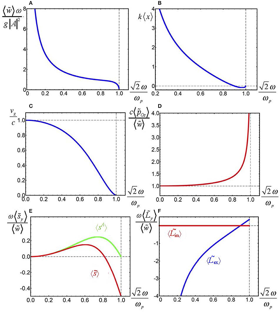
Figure 8. Frequency dependence of the main dynamical characteristic (DC) of the TM SPP wave (70), (71) for the electric and magnetic parameters of media 1 and 2 described by Equation (73) [52, 81]. (A) Integral energy (74); (B) center-of-gravity position (76); (C) group velocity (75); (D) orbital momentum (77); (E) SAM (79) (red line) and the “traditional” Abraham-type spin calculated without the dispersion corrections [53]; (F) intrinsic and extrinsic (with respect to the interface x = 0) OAM (80).
By using the dispersion-modified definitions (48)–(51), the SPP energy is expressed in the form:
where
is the SPP group velocity [cf. Equations (11) and (12) and Figures 8A,C]. Note that under certain conditions (not realized in Figure 8C), vg can be negative (the wave field (70), (71) propagates toward z → +∞, while the SPP energy flows oppositely [39, 100]).
The SPP confinement enables a meaningful definition of the center of gravity (21) (see Figure 8B):
The OM of the SPP is completely longitudinal and fairly agrees with Equation (66):
(Figure 8D), which, again, means that the SPP carries supermomentum [12, 21, 53] hks > hk per polariton, both locally and integrally [52, 81].
The SM density (51) consists of three parts (Figure 9). In the upper half-space, the usual SM (65) of the EW in a dielectric is directed oppositely to the wave propagation (green arrows in Figures 7C, 9). In the lower half-space, the EW is formed in the conductive medium, and the SAM is coupled to the circulatory motion of the charge carriers (electrons) schematically shown in Figure 9. Accordingly, the SM (yellow arrow in Figure 9) includes the mechanical momentum of electrons. As in other similar cases [67, 69, 70], a linear macroscopic current emerges in the system of inhomogeneously distributed microscopic vorticities due to the incomplete compensation of oppositely directed electron velocities in adjacent horizontal layers of medium 2. The compensation is completely destroyed at the interface where the sequence of electron loops “breaks,” and the near-surface motions of electrons “combine” into a strictly localized z-directed momentum (red arrow in Figure 9): this is the third part of the SM. In agreement with the general theory [see equation (22)], the three parts of the SM mutually cancel out, : that is why the integral SM is not illustrated in Figure 8.
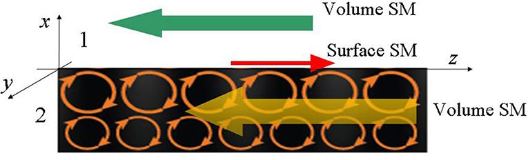
Figure 9. Illustration of the elliptic trajectories of electrons and the SM constituents [82]. The ellipses' sizes and the electron velocities decay with the off-surface distance in the half-space x < 0.
An important aspect of this behavior is that the material SAM and SM contributions in medium 2 are formed by the charged particles and are, therefore, associated with electric currents. As a result, the SPP-induced magnetization (a sort of inverse Faraday effect) [83] must appear in the conductive medium 2 [52, 81, 82]. Its quantitative measure (the magnetic moment of the conductive-medium layer per unit z-length and unit y-width) can be presented in the form [39]:
where e < 0 and me are the electron charge and mass. Noteworthy, the magnetization effect is of essentially dispersive nature and vanishes when .
In contrast to the EW formed upon total reflection [see Equation (63)], the SAM of the SPP is purely transverse:
Figure 8E shows that the SAM can have different directions at different frequencies and, in case of the Drude model (73), vanishes for . According to Equations (19) and (20) and the second Equation (50), the OAM density of the SPP field reduces to , that is, the intrinsic OAM [with respect to the center of gravity (76)] vanishes, and the extrinsic OAM (with respect to the coordinate origin) equals:
The vanishing intrinsic OAM part means that the OM of the SPP does not exhibit any vortex-like circulation, in contrast to the Poynting–Abraham energy flux [53, 104].
Applications of Structured Light
The unique properties of structured light are now extensively used in many scientific and technological fields, and still more new applications are developed every day in laboratories. Here, we consider some selected applied aspects of structured light that can illustrate their general fundamental properties and physical nature.
Structured Light in Optical Tweezers and Micro-Manipulation Techniques
After 1970 when Ashkin [105] (the Nobel Prize 2018) had revealed the focused laser beam's ability of exerting a mechanical action on small particles, the technique of optical manipulation demonstrated a huge progress, and all this development has been associated with the properties of structured light. The diversity of relevant methods and instruments is almost boundless, and in this paper, we can only mention the main principles and illustrate the peculiar mechanisms or the structured light properties employed for spatial localization and transportation of micro- and nanoobjects [8, 11, 38, 64, 68, 106–113].
The first idea realized in the early works by Ashkin is based on the inhomogeneous energy distribution and the gradient force [first summands of Equations (23)]. Owing to this, a dielectric particle, whose refractive index exceeds that of the environment, tends to be localized in the intensity maxima; correspondingly, the particles with small refractive index, as well as absorbing particles, move to the intensity minima, which form thus the “gradient optical traps.” This mechanism provides efficient means for the 3D particle localization and controllable displacement with the help of “bottle beams” that contain volumes of low (zero) intensity surrounded by the high-intensity regions [111–118] (Figure 10). The generic bottle beam configuration is illustrated in Figures 10a,b. Such beams can be generated, e.g., by superposition of oppositely propagating OV beams [115] or inside the focal volume of a lens with a controlled spherical aberration [117]. Further development of these principles has led to the creation of multiple optical traps (Figure 10c) able to manipulate ensembles of trapped particles in air [114, 116–120].
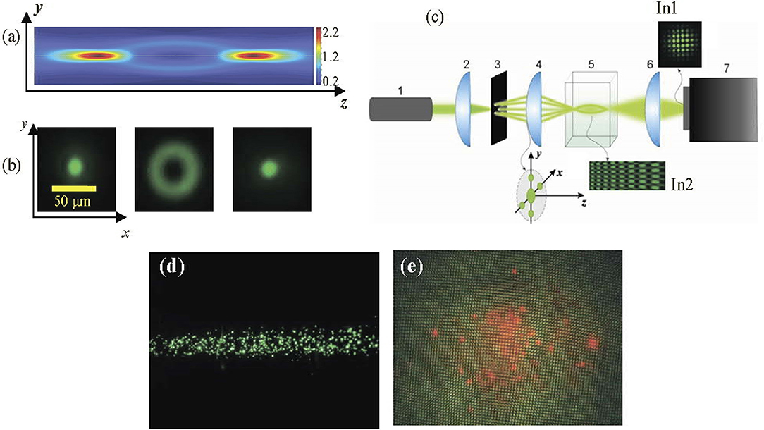
Figure 10. (a) Longitudinal and (b) transverse cross sections of a bottle beam. (c) Experimental setup for generation of the regular set of 3D optical traps [118]: laser 1 emits radiation with λ = 532 nm, which through the collimating lens 2, the amplitude transparency (2D diffraction grating) 3 and microscopic objective 4 enters cuvette 5 with carbon particles. The lens 6 projects the cuvette interior into the CCD camera 7. Insets In1 and In2 show the longitudinal and transverse intensity distribution in the multiple-trap beam. (d,e) Longitudinal and transverse views of the beam in the cuvette with trapped particles [in (e), the particles are additionally illuminated by the red laser].
Other popular types of optical traps additionally exploit the rotational properties of structured light beams enabling controlled transverse motion and orientation of particles [7, 57, 68, 106, 110, 121]. For example [121], a focused multi-ring OV beam with linear polarization traps particles suspended in water within a bright ring (the particle localization along the longitudinal direction is performed by non-optical means due to the cell construction) and causes their orbital motion along the ring by means of the transverse light-pressure component (23) (Figure 11B). This can be considered as a direct manifestation of the beam OAM (see the Optical Vortices section and the General Definitions subsection). When the incident beam is circularly polarized, a particle additionally experiences optical torque (26) resulting from the beam's SAM and inducing the spinning motion (Figure 11C).
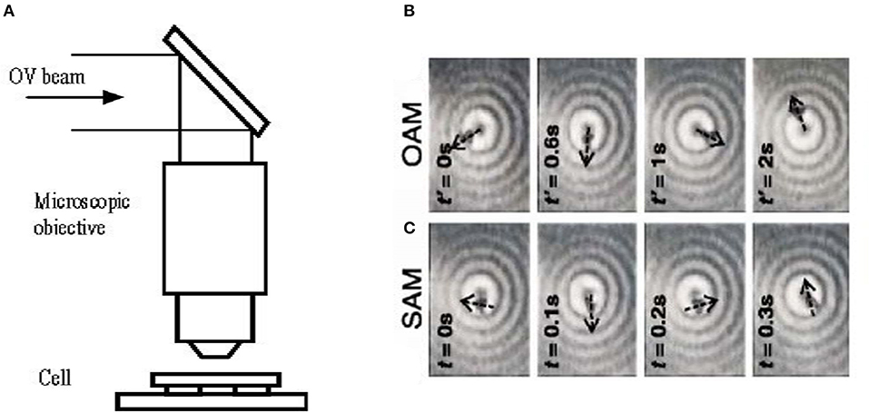
Figure 11. (A) Optical system focusing the beam with OAM into the cell with suspended particles; (B,C) consecutive time-dependent positions and orientations of the particles in the objective focal plane under the action of the beam with (B) OAM, and (C) SAM [121].
The principle of Figure 11A can be used in optically driven sensors and machines for micro-fluidic environments, for fine adjustment of selective chemical interactions, in studies of the fluid and particle's properties [110]. In other approaches [64, 106, 107], the structured fields with inhomogeneous polarization are suggested for creation of easily controllable and technically flexible optical traps (Figure 12).
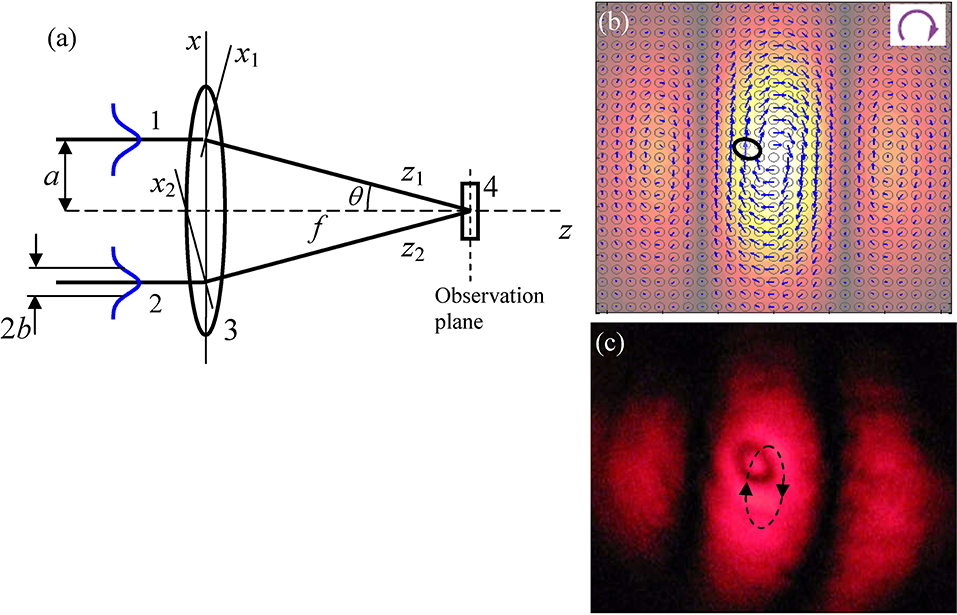
Figure 12. (a) Experimental scheme for realization of optical trap with inhomogeneous polarization [64, 106]: 1 and 2 are the input beams, 3 is the objective lens, the cuvette 4 with water-suspended particles is placed in the focal plane. (b) Simulated and (c) experimental pictures observed in the cuvette; (b) the particle trace is conventionally presented by the black oval; arrows show the transverse SM lines [cf. Equation (29)] in the case of right circular polarization of the input beams (indicated in the right upper corner); (c) the dashed oval with arrows schematically illustrates the particle trajectory.
In this scheme, the trap is formed due to the interference of beams 1 and 2 whose polarization (circular, elliptic, linear), phase, intensity, and degree of mutual coherence can be varied in a wide range by means of the polarization interferometry techniques [122–124]. In the simplest scheme [64], two identical Gaussian beams from a semiconductor laser (λ = 0.67 μm) with radii b = 0.7 mm (measured at the intensity level e−1 of maximum) approach a micro-objective with a focal distance of f = 10 mm (Figure 12a). The beams are parallel to the objective axis and are located at a distance a = 1.3 mm from it, which provides the effective focusing angle θ = arctan(a/f) ≈ 7.4° and NA ~ 0.16; after focusing, they interfere in the focal region of the objective where the cuvette with liquid-suspended particles is placed. At the lens 3 input (see Figure 12a), beams 1 and 2 possess the complex amplitude distributions:
Behind the objective, each beam propagates along its own axis zj with focusing angle ~ arctan(b/f) ≈ 0.07 rad, which practically corresponds to the paraxial regime with the paraxiality parameter γ = b/f (see the Principles of the Structured Light Description: Paraxial Model section). Therefore, in the proper coordinate frame (xj, yj, zj) (see Figure 1), which is connected to the laboratory frame (x, y, z) by the relations:
the beams' evolution is described by the equation readily derived from Equation (81) and the common theory of Gaussian beams (see, e.g., [8, 11]):
where the coefficient η accounts for the energy losses in the focusing optical system, and (see the Principles of the Structured Light Description: Paraxial Model). Then, neglecting the small longitudinal components, which appear due to the oblique incidence (this is possible because the longitudinal localization of a particle is regulated by the mechanical confinement, e.g., by the cuvette walls), the resulting amplitude distribution in the focal region can be found from the equation:
where δ specifies the exact location of the observation plane with respect to the focus (normally, δ can be adjusted to provide the best conditions for particle trapping and manipulation), zj and xj should be replaced by their expressions (82), with allowance for z = f + δ.
The dynamical properties of the interference pattern are determined by Equations (23), (24), (26), and (82)–(84) for conditions of Figure 12a and are illustrated in Figure 12b for the case of circularly polarized beams 1 and 2. According to the Dynamical Characteristics of the Paraxial Fields section, the SM is directed along the constant-intensity lines and forms circulatory flows within each lobe, while the transverse component of the orbital (canonical) momentum (35) is attributed to the beam (84) divergence and directed off-center. Adjusting the angle θ, focal length f , and the relative phase of the beams enables independent regulation of the intensity pattern and the spatially inhomogeneous polarization of the field in the observation plane. In experiments, a latex particle (n = 1.48) suspended in water was trapped within the central lobe at a certain distance from the axis due to equilibrium between the gradient force “pulling” it to the intensity maximum and the OM-induced light pressure “pushing” it out [64]. In the case of the circular polarization, an asymmetric particle spins due to the spin-induced torque (26). Simultaneously, it performs an orbital motion (dashed elliptic trajectory in Figure 12c) due to the transverse SM (29) and the corresponding force component [first summand of (24)]. The sense of orbiting reverses with the sign of circular polarization; in case of linear polarization, the particle's motion stops. Note that the OM in the first summand of Equation (24) cannot cause the particle orbiting in the scheme in Figure 12 because of its off-center direction, and thus, the “pure” mechanical action of the SM is observed [cf. the General Definitions subsection, paragraph above Equation (25)].
Additional fruitful possibilities in optical manipulation techniques are supplied by the evanescent fields. In an EW, a particle is efficiently trapped in one dimension by the very field configuration but can be shifted, translated, orbited, and spun by the ponderomotive factors described by Equations (62)–(67) and (69) [88–90, 125–127]. A great variety of elliptical trajectories of fluid-suspended microparticles driven by a single evanescent field has been observed [125–127]. This behavior is highly tunable and agrees with the theoretical model that accounts for Mie scattering and hydrodynamic drag. It shows that the structured-light approaches are useful for inducing orbital motion of microparticles, with readily tunable parameters of motion including orbital frequency, radius, and ellipticity [127]. Additionally, in many cases, the EW-generated optical forces, intrinsically related with the wave helicity, exert selective influences with respect to the particle chiral properties, thus, enabling the chirality-dependent manipulation and sorting [125, 126]. This promises especial facilities in biomedical applications [88–90]. Further deeper understanding of the detailed dynamics of microparticles in a fluidic environment near a surface will contribute to effective application of optically driven microparticles as functional elements in optofluidic devices.
Optical Switching and Signal Processing: Applications of the EW and SPP Properties
Evanescent optical waves and, especially, SPPs attract enormous interest during the recent decades for many reasons, but the most important—in our opinion—is the fact that these offer promising ways for creation and development of all-optical information-processing systems. Practical realization of very attractive optical methods for the information encoding, delivering, and processing with usual optical elements meets a natural limitation. Since an optical field cannot be localized in a volume less than the wavelength size, the optical gates, switches, triggers, etc., seemingly cannot compete with the solid-state counterparts in microminiaturization potential. And only the near-field optics, first of all plasmonics, enables manipulation of “bulky” optical fields with “tiny” subwavelength elements with the nanometer-size scales.
In this view, the possibilities for the controllable SPP excitation and propagation are in the focus of current research [12, 95]. Most of them are associated with the transverse spin–momentum locking, or coupling [Equations (63), (64)], and a number of prominent results has been reported [91–94, 128–132]. Despite the different setups and interfaces, all of the recent experiments explore the same physical principles discussed in the Evanescent Waves: Extraordinary Spin and Momentum section and the Surface Plasmon-Polaritons section (see Figure 13). In all these cases, external y-propagating light beam with usual longitudinal SAM from the circular polarization (σ= ± 1) is coupled to surface EWs propagating along the z-axis via the interaction with some scatterer (nanoparticle, atom, etc.). Since the SAM of the incident wave has to match the y-directed transverse SAM in EWs, opposite incident helicities (σ = 1 and σ = −1) generate unidirectional EWs propagating in opposite z-directions (kz > 0 and kz < 0), respectively. Thus, such a strong and robust spin-direction locking offers perfect “chiral unidirectional interfaces,” potentially important for many applications, such as quantum information [92, 93], topological photonics [95, 133], and chiral spin networks [134]. Note that the spin-direction coupling is reversible, i.e., the transverse emission of propagating light from oppositely propagating EWs has opposite circular polarizations (spins) [129].
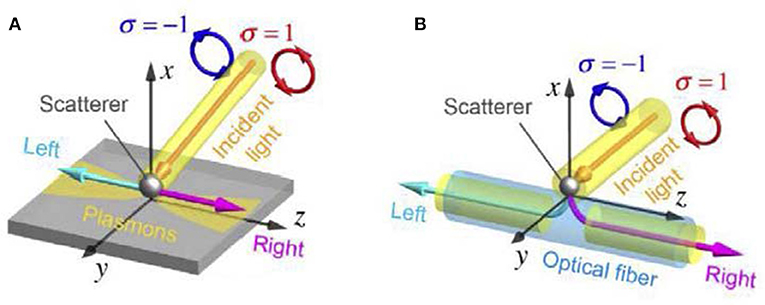
Figure 13. Spin-controlled unidirectional coupling of light to oppositely propagating modes: (A) in the planar geometry; (B) excitation of an optical-fiber-guided mode (the figure is adapted from the presentation by K. Bliokh, © 2017).
Specific magnetic properties of the SPPs open additional opportunities in optical commutation techniques. For example, combining transverse spin-direction locking with the spin-dependent magnetooptical scattering or absorption [128] results in an efficient “optical diode,” i.e., non-reciprocal transmission of light [130]. The presence of the SPP-induced magnetization (78) leads to the non-reciprocical magneto-plasmonic spectrum in an applied magnetic field [135, 136] (which is usually explained via the permittivity tensor anisotropy caused by the external magnetic field [137]). Really, the magnetization (78) means that each SPP quasiparticle carries the magnetic moment . Therefore, applying the transverse magnetic field H0 = H0ey leads to the Zeeman interaction shifting the SPP frequency:
where Ω = −eH0/mec is the cyclotron frequency of electrons, ω0(ks) is the “standard” dispersion law expressed by the first Equation (72), and the conditions of the simplified media's model (73) are employed. As a result, the SPP spectrum becomes non-reciprocal, i.e., depending on the propagation direction expressed by sgn (ks) (Figure 14A). In particular, the cutoff frequency is now shifted to sgn (ks)Ω/2, and for frequencies between and , SPPs become unidirectional, i.e., propagating only in the positive (negative) z-direction, depending on the H0 sign.
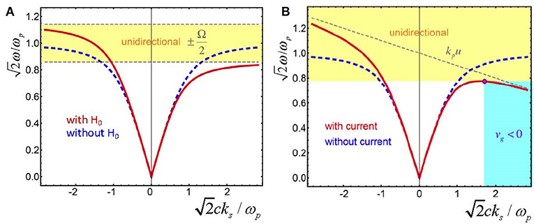
Figure 14. Non-reciprocal modifications of the SPP spectra caused by (A) a transverse magnetic field, Equation (85), and (B) a longitudinal direct electric current, Equation (86) (reprinted with permission from Bliokh et al. [99] ©2018 The Optical Society). The dashed curves show the unperturbed reciprocal SPP dispersion ω0(ks) for the Drude model (73). The frequency ranges with the one-way SPP propagation and the wavevector range with the negative group velocity of SPPs are marked by yellow and blue, respectively. The parameters are (A) Ω = 0.2ωp and (B) u = −0.1c.
A similar effect appears in the presence of electric current I in the conductive part of the SPP-supporting structure [99]. Indeed, the current means that free electrons move with the velocity u = I/(nee) (remember that e < 0), where is the density of the electrons. This motion of the electron plasma produces the Doppler frequency shift ω → ω – ksu in the metal permittivity (73) and the corresponding modification of the dispersion law:
(see Figure 14B). Except for the non-reciprocity, the electric current creates possibilities for the zero and negative group velocity of the SPP dω/dks. The described effect may occur not only in planar structures like in Figure 7C but also in the cylindrical geometry, which can be more practical. Numerical estimations [99] show that for a nanowire with ωp = 1016 s−1 and radius 20 nm, an electric current I = 0.5 mA provides quite realizable conditions for unidirectional propagation of SPPs with frequencies differing from the cutoff value approximately by δω = ±1010 s−1 (although the unidirectional-propagation range theoretically is not limited from above, see Figure 14B, high wave numbers ks are usually accompanied by strong SPP absorption [85, 86]).
The ability to achieve one-way optical propagation using direct electric currents is conceptually simple and inherently compatible with modern microelectronics industry, does not require bulky external magnets, and can be easily implemented in an on-chip integrated environment, potentially combining electrical and optical components.
Structured Light in Telecommunication and High-Resolution Techniques
Carrying information is one of the most evident structured-light functions. Actually, any optical image can be considered as structured light carrying information in an analog form, but more important is the possibility of light structures to encode digital data. Natural means for this are supplied by the discrete states of light, which can be realized in its spatial and/or polarization degrees of freedom. For example, the binary information can be easily encoded by two possible states of circular polarization [2] as well as by discrete set of OV-carrying modes differing by the topological charges; in the latter case, the multidimensional quantum space with the orthogonal functional basis becomes real [138, 139].
Structured light fields enable substantial increase in the communication bandwidth due to multiplexing of several independent information flows within a single channel. Traditional sorts of multiplexing [polarization-division multiplexing (PDM) and wavelength-division multiplexing (WDM)] can be supplemented by the spatial-division techniques (SDM) in which several independent beams are transmitted simultaneously. A sort of SDM is the mode division multiplexing (MDM), where each beam is transmitted in its unique spatial mode, and these modes are orthogonal to each other, providing efficient multiplexing and low cross-impact. The SDM regime is compatible with the PDM and WDM regimes and their simultaneous combinations may offer additional advantages. Particularly, the orthogonal sets of circular OV beams (see the Optical Vortices section) with different topological charges supply a characteristic example of the MDM channel where a number of independent beams propagate along the same path with no or negligible cross-talk [138, 139]. Owing to the circular symmetry, such beams are practically suitable and compatible with usual optical systems.
Explicit employment of the structured light properties enables essential progress in the quality and efficiency of “traditional” classical information channels. Specific features of singular light fields make possible a substantial compression of the transmitted information encoded in the light spatial structure. This can be implemented due to the sign principle of singular optics [11, 27, 29, 32]. The field behavior in the regions “filling” the singular skeleton (e.g., between the OV cores in scalar fields and between the C-points and s-contours in vectorial ones) can be restored with high accuracy, once the singular skeleton itself is known. This circumstance permits the information to be “economically” encoded in the singular-skeleton features of coherent fields; additional details of the field behavior can be recovered with high quality. It was shown that the full optical information can be reliably restored even if the real volume of transmitted data is decreased up to 15 orders of magnitude. Such a degree of information compressing is unique for complex 2D signals and provides high communication bandwidth with impressive transmission security.
Important questions appear relating the applicability of the developed approaches to the partially coherent and partially polarized structured fields. First results (e.g., [140, 141]) testify that reliable data encoding with partially coherent light is quite possible, and efficient algorithms for the compressed encoding and the full information retrieval are available and offer some practical benefits.
Another important (and, probably, unique) advantage of structured light relates to the quantum information processing. Any coherent light field can be prepared in a single-photon state, and all the specific quantum-information instruments (coherence, superposition, quantum measurements) can be realized in the most direct and simple way. In the simplest case (quantum communications [2]), the encoding–decoding actions are minimal. Another processing problem appears in the quantum calculations; however, at present, the techniques of quantum computation with structured light is only in its initial stage [142–144]. The basis for quantum computing is the quantum teleportation, which employs the entangled states, for example, those uniting the spin and spatial degrees of freedom (see, e.g., [145, 146]).
High-dimensional quantum encoding opens up attractive prospects for improving the quantum communication protocols, development of superdense encoding and schemes of the quantum key distribution [2]. Physical realization of such schemes is based on the utilization of light modes with a well-developed structure. Recent works demonstrate the efficiency of the structured-light modes for systems of ultra-fast switching and commutation of the information channels. Structured light fields are efficient in quantum high-dimensional cryptography [2]. Optical technologies for generation, manipulation, and detection of quantum states, whose superposition is encoded in the light structure, enable useful applications in quantum communication.
The problems of structured vector fields are closely related to other interesting questions associated with highly structured (tailored) vector beams [147–150], high-resolution Stokes polarimetry and 3D polarimetric analysis. In these areas, the impressive results were associated with the focusing properties of radially and azimuthally polarized beams (“cylindrical vector beams”). In the focal regions of such beams, the electromagnetic “needles” are formed along the propagation axis, whose width is lower than the usual diffraction limit available, e.g., for a standard Gaussian beam. This important result is attractive for applications in nanolithography, optical nano-probing, as well as ultra-high density optical data storage; also, such fields can be applied for detection and measurements of small mechanical rotations [2].
On the other hand, such “super-focused” beams put forward new problems for the standard Stokes-polarimetry techniques oriented at the paraxial fields. In case of super-focusing, the true 3D distribution of the electric and magnetic vectors should be taken into account. For measurements of the separate polarization components, including the longitudinal one, in tightly focused beams, the individual fluorescent molecules with fixed molecular axis are employed [2]. Further, it has been demonstrated that the near-field tips developed for the near-field scanning optical microscopy can be utilized to map confined fields and to distinguish between individual polarization components. With this technique, the phase distributions of the electric field components were measured using an interferometric detection approach.
The full vector pattern of the focused beam can be mapped by means of a nanoparticle used as an instrument for field scanning [2, 151]. The field scattered by the nanoparticle interferes with the incident (exciting) field, and the information on the electric field components is contained in the interference patterns. As a result, the phase and amplitude distributions of the focused field are derived from the measured angular far-field intensity distribution. Therefore, experimental study of highly structured fields with excellent resolution becomes possible. Nevertheless, the need for the development of efficient, fast, and miniature devices for generation, detection, and sorting of structured light beams is called for.
Another sort of fields with 3D polarization distribution is represented by Poincaré beams whose cross sections show all possible polarization states with a polarization singularity (C-point) on the axis. This singularity is coupled with the OV for one of the opposite circular polarization components; the field, itself, does not vanish in the polarization core but a certain circulatory component of the energy flow still exists [10]. With further propagation, the polarization pattern of the beam changes but in a predictable regular way. In the quantum regime, photons with space-varying polarization can be treated as non-separable (“entangled”) quantum states of the polarization and spatial degrees of freedom. Such a form of single-particle entanglement can be used for the quantum information protocols [2, 152]. Photons, for which the polarization ellipse can have arbitrary 3D position and orientation, can be efficiently utilized for long-distance quantum communication, especially when the influence of medium turbulence and of the beam divergence is substantial.
In general, current results, relating the generation, manipulation, and measurements of structured fields with complex polarization morphology, enable many applications such as recording and reading information with high-resolution, high-bandwidth secure communication, optical metrology, etc. Three-dimensional structured vector fields will enable an innovative platform for subwavelength lithography and selective excitation of structured matter with complex topology.
Conclusion
To conclude this brief review, we emphasize that the “structured light” is a very wide and rapidly expanding field. Nowadays, the structured-light studies form a separate chapter of modern optics whose formulation and detailed specification is still “in preparation.” Only a small part of the structured-light-related facts and concepts have been reflected in this paper.
However, in this review, we tried to give, if not exhaustive, but a rather representative characterization of the dynamical characteristics (energy, momentum, angular momentum, and related quantities) of structured light. This choice was dictated by our belief that it is the dynamical characteristics that form an adequate system of the structured-light parameters enabling its natural description, which is both physically consistent and suitable for applications. Some special kinds of structured light, namely, paraxial beams (including optical vortices) and evanescent waves are considered in more detail due to their practical importance and descriptive abilities demonstrating some general principles by means of the simple and physically intuitive examples. Also, we have outlined selected applications of structured light fields where their exclusive properties act in the more direct and immediate way: principles and techniques of optical micromanipulation, optical diagnostics and microprobing, optical switching and commutation, communication and data processing.
However, structured light is a much wider concept, and many interesting aspects remain beyond the scope of this review. Together with the “pure light” aspects, such as phase and polarization singularities, inhomogeneous amplitude, and extraordinary dynamical properties, the structured light offers a wide variety of new possibilities, associated with diverse light–matter interactions. Realization of these possibilities leads to noticeable advances, e.g., in the atomic and electron physics. Among the promising lines of further development, we can mention the wider employment of fields with complex polarization topology and 3D vector structure, more extensive utilization of artificial media and metamaterials. Essential advances are expected from consistent realization of a novel paradigm that can be characterized as “structured light in structured media.” In particular, this will bring new, more flexible, and universal methods for the purposeful generation of light fields with desirable structure for more precise micromanipulation, optical diagnostics, efficient data storage, and processing.
Nevertheless, despite the impressive results and applications, the structured light physics would have a limited scientific interest, if it had no influence on other areas of science and technology. The inter-disciplinary impact of structured-light optics is clearly manifested in metrology and communication techniques, nanophotonics, quantum physics, astronomy, microscopy, biology, and chemistry. Moreover, the concepts and paradigms of structured-light optics find new and sometimes unexpected applications to different kinds of electromagnetic fields, electron waves, acoustic waves, and to the most fundamental problems, including the nature of physical fields and the general wavefield concepts.
Author Contributions
OA, CZ, and SH contributed in the conception and design of the study. AB and JZ organized the database. CZ wrote the first draft of the manuscript. IM and AB wrote sections Principles of the Structured Light Description: Paraxial Model and Sorts of Structured Light. AB and SH wrote sections Dynamical Characteristics of Structured Optical Fields and Evanescent Waves: Extraordinary Spin and Momentum. JZ and AB contributed to section Surface Plasmon–Polaritons. OA, AB, and CZ wrote section Applications of Structured Light. All authors contributed to the manuscript revision, read, and approved the submitted version.
Funding
This work was supported, in part, by the Ministry of Education and Science of Ukraine (project 582/18, #0118U000198).
Conflict of Interest
The authors declare that the research was conducted in the absence of any commercial or financial relationships that could be construed as a potential conflict of interest.
The reviewer FN declared a past co-authorship with one of the authors AB to the handling editor.
References
2. Rubinsztein-Dunlop H, Forbes A, Berry MV, Dennis MR, Andrews DL, Mansuripur M, et al. Roadmap on structured light. J Opt. (2017) 19:013001. doi: 10.1088/2040-8978/19/1/013001
3. Andrews DL. Structured Light and Its Applications: An Introduction to Phase-Structured Beams and Nanoscale Optical Forces. Amsterdam: Academic Press. (2011).
4. Litchinitser NM. Structured light meets structured matter. Science. (2012) 337:1054–5. doi: 10.1126/science.1226204
5. Woerdemann M. Structured Light Fields: Applications in Optical Trapping, Manipulation, and Organisation. Heidelberg: Springer Science & Business Media (2012). doi: 10.1007/978-3-642-29323-8_2
6. Xu Y, Sun J, Walasik W, Litchinitser NM. Probing metamaterials with structured light. Opt Express. (2016) 24:26249–54. doi: 10.1364/OE.24.026249
8. Bekshaev A, Soskin M, Vasnetsov M. Paraxial Light Beams With Angular Momentum. New York, NY: Nova Science Publishers (2008).
9. Bekshaev A, Bliokh K, Soskin M. Internal flows and energy circulation in light beams. J Opt. (2011) 13:053001. doi: 10.1088/2040-8978/13/5/053001
10. Bekshaev AY, Soskin MS. Transverse energy flows in vectorial fields of paraxial beams with singularities. Opt Commun. (2007) 271:332–48. doi: 10.1016/j.optcom.2006.10.057
11. Soskin MS, Vasnetsov MV. Singular optics. Prog Opt. (2001) 42:219–76. doi: 10.1016/S0079-6638(01)80018-4
12. Bliokh KY, Nori F. Transverse and longitudinal angular momenta of light. Phys Rep. (2015) 592:1–38. doi: 10.1016/j.physrep.2015.06.003
13. Bekshaev AY, Karamoch AI. Spatial characteristics of vortex light beams produced by diffraction gratings with embedded phase singularity. Opt Commun. (2008) 281:1366–74. doi: 10.1016/j.optcom.2007.11.032
14. McGloin D, Dholakia K. Bessel beams: diffraction in a new light. Contemp Phys. (2005) 46:15–28. doi: 10.1080/0010751042000275259
15. Karimi E, Zito G, Piccirillo B, Marrucci L, Santamato E. Hypergeometric-Gaussian modes. Opt Lett. (2007) 32:3053–55. doi: 10.1364/OL.32.003053
16. Roux FS. Distribution of angular momentum and vortex morphology in optical beams Opt. Commun. (2004) 242:45–55. doi: 10.1016/j.optcom.2004.08.006
17. Bekshaev A, Orlinska O, Vasnetsov M. Optical vortex generation with a “fork” hologram under conditions of high-angle diffraction. Opt Commun. (2010) 283:2006–16. doi: 10.1016/j.optcom.2010.01.012
18. Gbur G, Tyson RK. Vortex beam propagation through atmospheric turbulence and topological charge conservation. JOSA A. (2008) 25:225–30. doi: 10.1364/JOSAA.25.000225
20. Berry MV. Optical currents. J Opt A Pure Appl Opt. (2009) 11:094001. doi: 10.1088/1464-4258/11/9/094001
21. Berry MV, Shukla P. Geometry of 3D monochromatic light: local wavevectors, phases, curl forces, and superoscillations. J Opt. (2019) 21:064002. doi: 10.1088/2040-8986/ab14c4
23. Baranova NB, Zel'dovich BY, Mamaev AV, Pilipetskii NF, Shkunov VV. Dislocation density on wavefront of a speckle-structure light field. Sov Phys JETP. (1982) 56:983–7.
24. Logan BF Jr. Information in zero crossing of bandpass signals. Bell Syst Tech J. (1977) 56:487–510. doi: 10.1002/j.1538-7305.1977.tb00522.x
25. Nye JF, Berry MV. Dislocations in wave trains. Proc R Soc A. (1974) 336:165–90. doi: 10.1098/rspa.1974.0012
26. Nye JF. Natural Focusing and Fine Structure of Light: Caustics and Wave dislocations. Bristol; Philadelphia, PA: Institute of Physics Publishing (1999).
27. Mokhun II. Introduction to linear singular optics. In: Angelsky OV, editor. Optical Correlation: Techniques and Applications. Bellingham: SPIE Press (2007). p. 1–131. doi: 10.1117/3.714999.ch1
28. Strutt JW. Baron Rayleigh. Scientific papers (Vol. 3:1887-1892). Cambridge: University Press (1899-1920), reissued by the publisher 2011, ISBN 978-0-511-70398-0.
29. Freund I, Shvartsman N. Wave-field singularities: the sign principle. Phys Rev. (1994) 50:5164–72. doi: 10.1103/PhysRevA.50.5164
30. Freund I, Shvartsman N, Freilikher V. Optical dislocation networks in highly random media. Opt Commun. (1993) 101:247–64. doi: 10.1016/0030-4018(93)90375-F
31. Galushko Yu, Mokhun I. Characteristics of scalar random field and its vortex networks. Recovery of the optical phase. J Opt A: Pure Appl Opt. (2009) 11:094017. doi: 10.1088/1464-4258/11/9/094017
32. Angelsky OV, Gorsky MP, Hanson SG, Lukin VP, Mokhun II, Polyanskii PV, et al. A Optical correlation algorithm for reconstructing phase skeleton of complex optical fields for solving the phase problem. Opt. Express. (2014) 22:6186–93. doi: 10.1364/OE.22.006186
33. Rubinov AN. Physical grounds for biological effect of laser radiation. J Phys D Appl Phys. (2003) 36:2317–30. doi: 10.1088/0022-3727/36/19/002
34. Popov AY, Popova NA, Tyurin AV. A physical model of the action of low-intensity laser radiation on biological objects. Opt Spectrosc. (2007) 103:671–77. doi: 10.1134/S0030400X07100232
35. Sugic D, Dennis M. Singular knot bundle in light. JOSA A. (2018) 35:1987–99. doi: 10.1364/JOSAA.35.001987
36. Angelsky OV, Besaga RN, Mokhun II, Sopin MO, Soskin MS. Singularities in vectoral fields. Physics. (1999) 57:88–99. doi: 10.1117/12.370443
37. Mokhun AI, Soskin MS, Freund I. Elliptic critical points: C-points, a-lines, and the sign rule. Opt Lett. (2002) 27:995–7. doi: 10.1364/OL.27.000995
38. Dienerowitz M, Mazilu M, Dholakia K. Optical manipulation of nanoparticles: a review. J Nanophoton. (2008) 2:021875. doi: 10.1117/1.2992045
39. Bekshaev AY, Mikhaylovskaya LV. Electromagnetic dynamical characteristics of a surface plasmon-polariton. Optik. (2019) 186:405–17. doi: 10.1016/j.ijleo.2019.04.098
40. Bekshaev AY, Angelsky OV, Sviridova SV, Zenkova CY. Mechanical action of inhomogeneously polarized optical fields and detection of the internal energy flows. Adv Opt Technol. (2011) 2011:723901. doi: 10.1155/2011/723901
41. Bekshaev AY, Angelsky OV, Hanson SG, Zenkova CY. Scattering of inhomogeneous circularly polarized optical field and mechanical manifestation of the internal energy flows. Phys Rev A. (2012) 86:023847. doi: 10.1103/PhysRevA.86.023847
42. Bekshaev A, Soskin M. Transverse energy flows in vectorial fields of paraxial light beams. Proc. SPIE. (2007) 6729:67290G. doi: 10.1117/12.751952
43. Barnett SM, Loudon R. The enigma of optical momentum in a medium. Phil Trans Roy Soc A. (2010) 368:927–39. doi: 10.1098/rsta.2009.0207
44. Milonni PW, Boyd RW. Momentum of light in a dielectric medium, Adv Opt Photon. (2010) 2:519–53. doi: 10.1364/AOP.2.000519
45. Kemp BA. Resolution of the Abraham-Minkowski debate: Implications for the electromagnetic wave theory of light in matter. J Appl Phys. (2011) 109:111101. doi: 10.1063/1.3582151
46. Partanen M, Häyrynen T, Oksanen J, Tulkki J. Photon mass drag and the momentum of light in a medium. Phys Rev A. (2017) 95:063850. doi: 10.1103/PhysRevA.95.063850
47. Partanen M, Tulkki J. Mass-polariton theory of light in dispersive media. Phys Rev A. (2017) 96:063834. doi: 10.1103/PhysRevA.96.063834
48. Partanen M, Tulkki J. Mass-polariton theory of sharing the total angular momentum of light between the field and matter. Phys Rev A. (2018) 98:033813. doi: 10.1103/PhysRevA.98.033813
49. Partanen M, Tulkki J. Light-driven mass density wave dynamics in optical fibers. Opt. Express. (2018) 26:22046–63. doi: 10.1364/OE.26.022046
50. Bliokh KY, Bekshaev AY, Nori F. Extraordinary momentum and spin in evanescent waves. Nat Commun. (2014) 5:3300. doi: 10.1038/ncomms4300
51. Bekshaev AY, Bliokh KY, Nori F. Transverse spin and momentum in two-wave interference. Phys Rev X. (2015) 5:011039. doi: 10.1103/PhysRevX.5.011039
52. Bliokh KY, Bekshaev AY, Nori F. Optical momentum, spin, and angular momentum in dispersive media. Phys Rev Lett. (2017) 119:073901. doi: 10.1103/PhysRevLett.119.073901
53. Bliokh KY, Nori F. Transverse spin of a surface polariton. Phys Rev A. (2012) 85:061801. doi: 10.1103/PhysRevA.85.061801
54. Bekshaev A. Abraham-based momentum and spin of optical fields under conditions of total reflection. (2017). arXiv [Preprint]. arXiv:1710.01561.
55. Lee H-I, Mok J. Orbital and spin parts of energy currents for electromagnetic waves through spatially inhomogeneous media. J Mod Opt. (2018) 65:1053–62. doi: 10.1080/09500340.2017.1423407
56. Philbin TG, Allanson O. Optical angular momentum in dispersive media. Phys Rev A. (2012) 86:055802. doi: 10.1103/PhysRevA.86.055802
57. O'Neil AT, MacVicar I, Allen L, Padgett MJ. Intrinsic and extrinsic nature of the orbital angular momentum of a light beam. Phys Rev Lett. (2002) 88:053601. doi: 10.1103/PhysRevLett.88.053601
58. Philbin TG. Electromagnetic energy-momentum in dispersive media. Phys Rev A. (2011) 83:013823. doi: 10.1103/PhysRevA.83.013823
59. Belinfante FJ. On the current and the density of the electric charge, the energy, the linear momentum and the angular momentum of arbitrary fields. Physica. (1940) 7:449–74. doi: 10.1016/S0031-8914(40)90091-X
60. Bliokh KY, Bekshaev AY, Nori F. Dual electromagnetism: helicity, spin, momentum, and angular momentum. New J Phys. (2013) 15:033026. doi: 10.1088/1367-2630/15/3/033026
61. Bekshaev AY. Subwavelength particles in an inhomogeneous light field: Optical forces associated with the spin and orbital energy flows. J Opt. (2013) 15:044004. doi: 10.1088/2040-8978/15/4/044004
62. Nieto-Vesperinas M, Saenz JJ, Gomez-Medina R, Chantada L. Optical forces on small magnetodielectric particles. Opt Express. (2010) 18:11428–43. doi: 10.1364/OE.18.011428
63. Antognozzi M, Bermingham CR, Harniman RL, Simpson S, Senior J, Hayward R, et al. Direct measurements of the extraordinary optical momentum and transverse spin-dependent force using a nano-cantilever. Nat Phys. (2016) 12:731–5. doi: 10.1038/nphys3732
64. Angelsky OV, Bekshaev AY, Maksimyak PP, Maksimyak AP, Hanson SG, Zenkova CY. Orbital rotation without orbital angular momentum: mechanical action of the spin part of the internal energy flow in light beams. Opt Express. (2012) 20:3563–71. doi: 10.1364/OE.20.003563
65. Angelsky O, Bekshaev A, Maksimyak P, Maksimyak A, Hanson S. Measurement of small light absorption in microparticles by means of optically induced rotation. Opt Express. (2015) 23:7152–63. doi: 10.1364/OE.23.007152
66. Bliokh KY, Dressel J, Nori F. Conservation of the spin and orbital angular momenta in electromagnetism. New J Phys. (2014) 16:093037. doi: 10.1088/1367-2630/16/9/093037
67. Bekshaev AY. Spin angular momentum of inhomogeneous and transversely limited light beams. Proc SPIE. (2006) 6254:56–63. doi: 10.1117/12.679902
68. Bekshaev A, Vasnetsov M. Vortex flow of light: spin and “orbital” flows in a circularly polarized paraxial beam. In: Torres JP, Torner L, editors. Twisted Photons. Applications of Light with Orbital Angular Momentum. Weinheim: Wiley-VCH (2011). p. 13–24. doi: 10.1002/9783527635368.ch2
69. Mita K. Virtual probability current associated with the spin. Am J Phys. (2000) 68:259–64. doi: 10.1119/1.19421
70. Witting C. Photon and electron spins. J Phys Chem A. (2009) 113:15320–27. doi: 10.1021/jp906255u
71. Bekshaev AY. Role of azimuthal energy flows in the geometric spin Hall effect of light. (2011). arXiv [Preprint]. arXiv:1106.0982v1.
72. Bliokh KY, Nori F. Spin and orbital angular momenta of acoustic beams. Phys Rev B. (2019) 99:174310. doi: 10.1103/PhysRevB.99.174310
73. Aiello A, Banzer P, Neugebauer M, Leuchs G. From transverse angular momentum to photonic wheels. Nat Photon. (2015) 9:789–95. doi: 10.1038/nphoton.2015.203
74. Saha S, Ghosh N, Dutta Gupta S. Transverse spin and transverse momentum in structured optical fields. In: KGaA, ed Digital Encyclopedia of Applied Physics. Weinheim: Wiley-VCH Verlag GmbH & Co (2019). p. 1–32. doi: 10.1002/3527600434.eap818
75. Shi P, Du L, Li C, Zayats AV, Yuan X. Spin-momentum law for structured guided modes: the generalized quantum spin-Hall effect for light. (2019). arXiv [Preprint]. arXiv:1910.03904.
76. Gómez-Medina R, Nieto-Vesperinas M, Sáenz JJ. Nonconservative electric and magnetic optical forces on submicron dielectric particles. Phys Rev A. (2011) 83:033825. doi: 10.1103/PhysRevA.83.033825
77. Cardano F, Marrucci L. Spin-orbit photonics. Nat Photon. (2015) 9:776–78. doi: 10.1038/nphoton.2015.232
78. Neugebauer M, Bauer T, Aiello A, Banzer P. Measuring the transverse spin density of light. Phys Rev Lett. (2015) 114:063901. doi: 10.1103/PhysRevLett.114.063901
79. Bekshaev A. Spin-orbit interaction of light and diffraction of polarized beams. J Opt. (2017) 19:085602. doi: 10.1088/2040-8986/aa746a
80. Philbin TG. Lipkin's conservation law, Noether's theorem, and the relation to optical helicity. Phys Rev A. (2013) 87:043843. doi: 10.1103/PhysRevA.87.043843
81. Bliokh KY, Bekshaev AY, Nori F. Optical momentum and angular momentum in complex media: From the Abraham-Minkowski debate to unusual properties of surface plasmon-polaritons. New J Phys. (2017) 19:123014. doi: 10.1088/1367-2630/aa8913
82. Bekshaev AY, Bliokh KY. Spin and momentum of the light fields in inhomogeneous dispersive media with application to surface plasmon-polariton waves. Ukr J Phys Opt. (2018) 19:33–48. doi: 10.3116/16091833/19/1/33/2018
83. Landau LD, Lifshitz EM, Pitaevskii LP. Electrodynamics of Continuous Media. Oxford: Pergamon (1984). doi: 10.1016/B978-0-08-030275-1.50007-2
84. Bekshaev AY. Dynamical characteristics of an electromagnetic field under conditions of total reflection. J Opt. (2018) 20:045604. doi: 10.1088/2040-8986/aab035
85. Bertolotti M, Sibilia C, Guzman AM. Evanescent Waves in Optics: An Introduction to Plasmonics. Cham: Springer (2017). doi: 10.1007/978-3-319-61261-4
87. Zayats AV, Smolyaninov II, Maradudin AA. Nano-optics of surface plasmon polaritons. Phys Rep. (2005) 408:131–314. doi: 10.1016/j.physrep.2004.11.001
88. Angelsky OV, Hanson SG, Maksimyak PP, Maksimyak AP, Zenkova CY, Polyanskii PV, et al. Influence of evanescent wave on birefringent microplates. Opt Express. (2017) 25:2299–311. doi: 10.1364/OE.25.002299
89. Angelsky OV, Maksymyak PP, Zenkova CY, Maksymyak AP, Hanson SG, Ivanskyi DD. Peculiarities of control of erythrocytes moving in an evanescent field. J Biomed Opt. (2019) 24:055002. doi: 10.1117/1.JBO.24.5.055002
90. Angelsky OV, Zenkova CY, Maksymyak PP, Maksymyak AP, Ivanskyi DI, Tkachuk VM. Peculiarities of energy circulation in evanescent field. Application for red blood cells. Opt Memory Neural Netw. (2019) 28:11–20. doi: 10.3103/S1060992X19010028
91. Rodríguez Fortuño FJ, Marino G, Ginzburg P, O'Connor D, Wurtz GA, Martínez Abietar AJ, et al. Near-field interference for the unidirectional excitation of electromagnetic guided modes. Science. (2013) 340:328–30. doi: 10.1126/science.1233739
92. Petersen J, Volz J, Rauschenbeutel A. Chiral nanophotonic waveguide interface based on spin-orbit interaction of light. Science. (2014) 346:67–71. doi: 10.1126/science.1257671
93. le Feber B, Rotenberg N, Kuipers L. Nanophotonic control of circular dipole emission. Nat Commun. (2015) 6:6695. doi: 10.1038/ncomms7695
94. Söllner I, Mahmoodian S, Lindskov Hansen S, Midolo L, Javadi A, Kiršanske G, et al. Deterministic photon-emitter coupling in chiral photonic circuits. Nat Nanotechnol. (2015) 10:775–8. doi: 10.1038/nnano.2015.159
95. Bliokh KY, Smirnova D, Nori F. Quantum spin Hall effect of light. Science. (2015) 348:1448–51. doi: 10.1126/science.aaa9519
96. Bekshaev AY, Bliokh KY, Nori F. Mie scattering and optical forces from evanescent fields: A complex-angle approach. Opt Express. (2013) 21:7082–95. doi: 10.1364/OE.21.007082
97. Huard S, Imbert C. Measurement of exchanged momentum during interaction between surface-wave and moving atom. Opt Commun. (1978) 24:185–9.
98. Matsudo T, Takahara Y, Hori H, Sakurai T. Pseudomomentum transfer from evanescent waves to atoms measured by saturated absorption spectroscopy. Opt Commun. (1998) 145:64–8. doi: 10.1016/S0030-4018(97)00420-3
99. Bliokh KY, Rodríguez-Fortuño FJ, Bekshaev AY, Kivshar YS, Nori F. Electric-current-induced unidirectional propagation of surface plasmon-polaritons. Opt Lett. (2018) 43:963–6. doi: 10.1364/OL.43.000963
100. Shadrivov IV, Sukhorukov AA, Kivshar YS, Zharov AA, Boardman AD, Egan P. Nonlinear surface waves in left-handed materials. Phys Rev E. (2004) 69:016617. doi: 10.1103/PhysRevE.69.016617
101. Rakic AD, Djurisic AB, Elazar JM, Majewski ML. Optical properties of metallic films for vertical-cavity optoelectronic devices. Appl Opt. (1998) 37:5271–83. doi: 10.1364/AO.37.005271
102. Smith DR, Padilla W, Vier DC, Nemat-Nasser SC, Schultz S. Composite medium with simultaneously negative permeability and permittivity. Phys Rev Lett. (2000) 84:4184–7. doi: 10.1103/PhysRevLett.84.4184
103. Padilla WJ, Basov DN, Smith DR. Negative refractive index metamaterials. Mater Today. (2006) 9:28–35. doi: 10.1016/S1369-7021(06)71573-5
104. Shadrivov IV, Sukhorukov AA, Kivshar YS. Guided modes in negative-refractive-index waveguides. Phys Rev E. (2003) 67:057602. doi: 10.1103/PhysRevE.67.057602
105. Ashkin A. Optical Trapping and Manipulation of Neutral Particles Using Lasers. Singapore: World Scientific Publishing Company (2006). doi: 10.1142/4208
106. Angelsky OV, Bekshaev AY, Maksimyak PP, Maksimyak AP, Mokhun II, Hanson SG, et al. Circular motion of particles suspended in a Gaussian beam with circular polarization validates the spin part of the internal energy flow. Opt Express. (2012) 20:11351–56. doi: 10.1364/OE.20.011351
107. Angelsky OV, Bekshaev AY, Maksimyak PP, Polyanskii PV. Internal energy flows and optical trapping. Opt Photon News. (2014) 25:20–1.
108. Nieminen TA, Higuet J, Knoner G, Loke VLY, Parkin S, Singer W, et al. Optically driven micromachines: progress and prospects. Proc SPIE. (2006) 6038:237–45. doi: 10.1117/12.651760
109. Dholakia K, Reece P, Gu M. Optical micromanipulation. Chem Soc Rev. (2008) 37:42–55. doi: 10.1039/B512471A
110. Padgett M, Bowman R. Tweezers with a twist. Nat Photon. (2011) 5:343–8. doi: 10.1038/nphoton.2011.81
111. Arlt J, Padgett M. Generation of a beam with a dark focus surrounded by regions of higher intensity: the optical bottle beam. Opt Lett. (2000) 25:191–3. doi: 10.1364/OL.25.000191
112. Liu F, Zhang Z, Wei Y, Zhang Q, Cheng T, Wu X. Photophoretic trapping of multiple particles in tapered-ring optical field. Opt Express. (2014) 22:23716–23. doi: 10.1364/OE.22.023716
113. Zhao J, Chremmos ID, Song D, Christodoulides DN, Efremidis NK, Chen Z. Curved singular beams for three dimensional particle manipulation. Sci Rep. (2015) 5:12086. doi: 10.1038/srep12086
114. Shvedov VG, Desyatnikov AS, Rode AV, Krolikowski W, Kivshar YS. Optical guiding of absorbing nanoclusters in air. Opt Express. (2009) 17:5743–57. doi: 10.1364/OE.17.005743
115. Shvedov VG, Rode AV, Izdebskaya YV, Desyatnikov AS, Krolikowski W, Kivshar YS. Giant optical manipulation. Phys Rev Lett. (2010) 105:118103. doi: 10.1103/PhysRevLett.105.118103
116. Shvedov VG, Rode AV, Izdebskaya YV, Leykam D, Desyatnikov AS, Krolikowski W, et al. Laser speckle field as a multiple particle trap. J Opt. (2010) 12:1–8. doi: 10.1063/1.3507112
117. Shvedov VG, Hnatovsky C, Rode AV, Krolikowski W. Robust trapping and manipulation of airborne particles with a bottle beam. Opt Express. (2011) 19:17350–6. doi: 10.1364/OE.19.017350
118. Shvedov VG, Hnatovsky C, Shostka N, Rode A, Krolikowsky W. Optical manipulation of particle ensembles in air. Opt Lett. (2012) 37:1934–6. doi: 10.1364/OL.37.001934
119. Khoroshun A, Ryazantsev A, Ryazantsev O, Sato S, Kozawa Y, Masajada J, et al. Formation of an optical field with regular singular-skeleton structure by the double-phase-ramp converter. J Opt. (2020) 22:025603. doi: 10.1088/2040-8986/ab61c9
120. Khoroshun GM, Chernykh O, Tatarchenko HO, Sato S, Kozawa Y, Popiolek-Masajada A, et al. Chain of optical vortices synthesized by a Gaussian beam and the double-phase-ramp converter. OSA Continuum. (2019) 2:320–31. doi: 10.1364/OSAC.2.000320
121. Garcés-Chávez V, McGloin D, Padgett MJ, Dultz W, Schmitzer H, Dholakia K. Observation of the transfer of the local angular momentum density of a multiringed light beam to an optically trapped particle. Phys Rev Lett. (2003) 91:093602. doi: 10.1103/PhysRevLett.91.093602
122. Angelsky OV, Maksimyak PP, Magun II, Perun TO. On spatial stochastization of optical fields and feasibilities of optical diagnostics of objects with large phase inhomogeneities. Opt Spectr. (1991) 71:123–8.
123. Angelsky OV, Hanson SG, Zenkova CY, Gorsky MP, Gorodyns'ka NV. On polarization metrology (estimation) of the degree of coherence of optical waves. Opt Express. (2009) 17:15623–34. doi: 10.1364/OE.17.015623
124. Angelsky OV, Polyanskii PV, Mokhun II, Zenkova CY, Bogatyryova HV, Felde CV, et al. Optical measurements: polarization and coherence of light fields. In: Cocco L, editor. Modern Metrology Concerns. Rijeka: InTech (2012). p. 458.
125. Hayat A, Mueller JB, Capasso F. Lateral chirality-sorting optical forces. Proc Natl Acad Sci USA. (2015) 112:13190–4. doi: 10.1073/pnas.1516704112
126. Rodríguez-Fortuño FJ, Engheta N, Martínez A, Zayats AV. Lateral forces on circularly polarizable particles near a surface. Nat Commun. (2015) 6:8799. doi: 10.1038/ncomms10263
127. Liu L, Kheifets S, Ginis V, Di Donato A, Capasso F. Elliptical orbits of microspheres in an evanescent field. Proc Natl Acad Sci USA. (2017) 114:11087–91. doi: 10.1073/pnas.1714953114
128. Mitsch R, Sayrin C, Albrecht B, Schneeweiss P, Rauschenbeutel A. Quantum statecontrolled directional spontaneous emission of photons into a nanophotonic waveguide. Nat Commun. (2014) 5:5713. doi: 10.1038/ncomms6713
129. O'Connor D, Ginzburg P, Rodríguez-Fortuño FJ, Wurtz GA, Zayats AV. Spin-orbit coupling in surface plasmon scattering by nanostructures. Nat Commun. (2014) 5:5327. doi: 10.1038/ncomms6327
130. Sayrin C, Junge C, Mitsch R, Albrecht B, O'Shea D, Schneeweiss P, et al. Optical diode based on the chirality of guided photons. Phys Rev X. (2015) 5:041036. doi: 10.1103/PhysRevX.5.041036
131. Lee SY, Lee I-M, Park J, Oh S, Lee W, Kim K-Y, et al. Role of magnetic induction currents in nanoslit excitation of surface plasmon polaritons. Phys Rev Lett. (2012) 108:213907. doi: 10.1103/PhysRevLett.108.213907
132. Miroshnichenko AE, Kivshar YS. Polarization traffic control for surface plasmons. Science. (2013) 340:283–4. doi: 10.1126/science.1236154
133. Lu L, Joannopoulos JD, Soljacic M. Topological photonics. Nat Photon. (2011) 8:821–9. doi: 10.1038/nphoton.2014.248
134. Pichler H, Ramos T, Daley AJ, Zoller P. Quantum optics of chiral spin networks. Phys Rev A. (2015) 91:042116. doi: 10.1103/PhysRevA.91.042116
135. Hu B, Wang QJ, Zhang Y. Broadly tunable one-way terahertz plasmonic waveguide based on nonreciprocal surface magneto plasmons. Opt Lett. (2012) 37:1895–7. doi: 10.1364/OL.37.001895
136. Davoyan AR, Engheta N. Electrically controlled one-way photon flow in plasmonics nanostructures. Nat Commun. (2014) 5:5250. doi: 10.1038/ncomms6250
137. Camley RE. Nonreciprocal surface waves. Surface Sci Rep. (1987) 7:103–87. doi: 10.1016/0167-5729(87)90006-9
138. Gibson G, Courtial J, Padgett M, Vasnetsov M, Pas'ko V, Barnett S, Franke-Arnold S. Free-space information transfer using light beams carrying orbital angular momentum. Opt Express. (2004) 12:5448–56. doi: 10.1364/OPEX.12.005448
139. Wang J, Yang J-Y, Fazal I M, Ahmed N, Yan Y, Huang H, et al. Terabit free-space data transmission employing orbital angular momentum multiplexing. Nat Photon. (2012) 6:488–96. doi: 10.1038/nphoton.2012.138
140. Polyanskii PV, Felde CV, Zelinskii YV, Konovhuk AV. On some prerequisites of correlation singular optics as a branch of information optics. Opt Memory Neural Networks. (2017) 26:207–15. doi: 10.3103/S1060992X17030067
141. Angelsky OV, Polyanskii PV, Maksimyak PP, Mokhun II. Metrology of coherence and polarization in sight of singular optics. In: Tuchin VV, editor. Handbook of Coherent-Domain Optical Methods: Biomedical Diagnostics, Environmental Monitoring, and Materials Science. New York, NY: Springer (2013). p. 67–106. doi: 10.1007/978-1-4614-5176-1_2
142. Wang X-L, Cai X-D, Su Z-E, Chen M-C, Wu D, Li L, et al. Quantum teleportation of multiple degrees of freedom of a single photon. Nature. (2015) 518:516–9. doi: 10.1038/nature14246
143. Nielsen MA, Chuang I. Quantum Computation and Quantum Information. New York, NY: Cambridge University Press (2000).
144. Knill E, Laflamme E, Milburn GJ. A scheme for efficient quantum computation with linear optics. Nature. (2001) 409:46–52. doi: 10.1038/35051009
145. Langford NK, Dalton RB, Harvey MD, O'Brien JL, Pryde GJ, Gilchrist A, et al. Measuring entangled qutrits and their use for quantum bit commitment. Phys Rev Lett. (2004) 93:053601. doi: 10.1103/PhysRevLett.93.053601
146. Krenn M, Huber M, Fickler R, Lapkiewicz R, Ramelow S, Zeilinger A. Generation and confirmation of a (100 ×100)-dimensional entangled quantum system. Proc Natl Acad Sci USA. (2014) 111:6243–7. doi: 10.1073/pnas.1402365111
147. Miyai E, Sakai K, Okano T, Kunishi W, Ohnishi D, Noda S. Photonics: lasers producing tailored beams. Nature. (2006) 441:946. doi: 10.1038/441946a
148. Otte E, Alpmann C, Denz C. Higher-order polarization singularitites in tailored vector beams. J Opt. (2016) 18:074012. doi: 10.1088/2040-8978/18/7/074012
149. Zhan Q, Leger JR. Focus shaping using cylindrical vector beams. Opt Express. (2002) 10:324–31. doi: 10.1364/OE.10.000324
150. Youngworth KS, Brown TG. Focusing of high numerical aperture cylindrical-vector beams. Opt Express. (2000) 7:77–87. doi: 10.1364/OE.7.000077
151. Bauer T, Orlov S, Peschel U, Banzer P, Leuchs G. Nanointerferometric amplitude and phase reconstruction of tightly focused vector beams. Nat Photon. (2014) 8:23–7. doi: 10.1038/nphoton.2013.289
Keywords: singular optics, optical vortex, polarization singularity, dynamical characteristics, paraxial beams, evanescent fields, optical manipulation, optical data processing
Citation: Angelsky OV, Bekshaev AY, Hanson SG, Zenkova CY, Mokhun II and Zheng J (2020) Structured Light: Ideas and Concepts. Front. Phys. 8:114. doi: 10.3389/fphy.2020.00114
Received: 20 January 2020; Accepted: 24 March 2020;
Published: 13 May 2020.
Edited by:
Shinichi Saito, University of Southampton, United KingdomReviewed by:
Konstantin Bliokh, RIKEN, JapanNobuhiko Yokoshi, Osaka Prefecture University, Japan
Franco Nori, RIKEN, Japan
Copyright © 2020 Angelsky, Bekshaev, Hanson, Zenkova, Mokhun and Zheng. This is an open-access article distributed under the terms of the Creative Commons Attribution License (CC BY). The use, distribution or reproduction in other forums is permitted, provided the original author(s) and the copyright owner(s) are credited and that the original publication in this journal is cited, in accordance with accepted academic practice. No use, distribution or reproduction is permitted which does not comply with these terms.
*Correspondence: Steen G. Hanson, vsgh@fotonik.dtu.dk