Dispersion in Fractures With Ramified Dissolution Patterns

1. Introduction

In both geological systems and industrial fields, fractures are known to be important pathways for fluid transport. Typically, the permeability of fractures is significantly higher than the porous matrix, so in many systems fractures play an important role in the fluid transport processes. The flow of tracer particles in a fracture is influenced by both convection and diffusion processes, and the combined effect of these two processes leads to Taylor dispersion. This effect was first studied by Taylor [1] for solvent flowing slowly through a tube. Afterwards it has been applied to various situations, for example, in single and parallel fractures [2, 3], in rough fractures [4], particle dispersion in narrow channels [5], and in a radial flow geometry [6, 7]. Some previous works consider geometric anisotropy, using self-organized percolation model to study flow through disordered porous media [8–10].

In most previous studies a flat open fracture with a constant aperture is considered, leading to a smooth and uniform front [11–15]. However in geological systems or industrial fields, such ideal initial states are rare. For example, when injecting a reactive fluid into an oil field, the injected fluid will react with the porous media which is stimulated by engineers trying to maximize the permeability around wells. A ramified dissolution pattern [16–18] will be formed around such an inlet. Those ramified features of the inlet will alter the fluid flow transport path in the rocks significantly. The flow transport problems in the fractures encountered in nature and in industry typically have irregular initial fronts, which is significantly different from the flat fronts obtained by injection into an open flat fracture. Considering a pollution leak problem for instance, if we suppose that the localized pollution source presents an initially uniform front in a homogeneous porous medium or aperture, we expect that the contamination spreads with radial symmetry, which deviates considerably from the actual situation because of the irregular initial front state. In this paper, we present experimental and numerical results demonstrating that with a ramified dissolution initial front state, in some directions the tracer will transport much faster than what we expect for an initially uniform front while in other directions there is no tracer transport at relatively long times.

In order to study these more realistic situations, a ramified dissolution pattern has been produced in a plaster sample, which is then used as the injection geometry. A fluid with a fluorescein tracer is injected into the cavity between this plaster sample and a flat plate, which together represent an open fracture. The injected fluid with tracer first fills the dissolved part and then starts flowing through the open fracture from the tips of dissolution fingers. The fluorescein tracer allows tracking of the flow radiating from this structure. We describe our experiments in section 2. In section 3, the simulation methods are illustrated. In section 4, the characteristics of the ramified dissolution patterns are studied. The experimental results are compared with results from numerical modeling in section 5. The conclusions follow in the last section.

2. Description of Experiments

The experimental setup is illustrated in Figure 1. The experiments were performed in a Hele Shaw cell which consists of two circular and parallel flat glass plates. The bottom glass plate (Diameter d₁ = 36.0 cm) is larger than the upper one (Diameter d₂ = 25.0 cm) and has an external rim. An inlet is located at the center of the lower glass plate, and the two glass plates are separated by aluminum spacers of thickness b = 1.00 mm and held together by clamps.

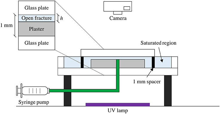
Figure 1. Schematic diagram of experimental setup. A circular Hele Shaw cell (spacing 1 mm) contains a saturated plaster plate with a small gap (h = 50.0 μm) above the plaster. A tracer fluid is injected by a syringe pump into the center of the Hele Shaw cell, where it flows radially outwards. The model is illuminated from below by an ultraviolet light source. The plaster plate has a fixed dissolution pattern around the injection point, formed by distilled water injection before the tracer injection experiment.

2.1. Sample Preparation

In the experiments we study the dispersion phenomena in an open fracture with an initial state representing a ramified dissolution pattern. We therefore first created a dissolution pattern in the sample, and later performed the tracer dispersion experiment. The plaster sample with a dissolution pattern on the top surface was prepared by the following steps:

A plaster saturated water solution was first injected into the Hele Shaw cell. Water and plaster powder (Alabaster plaster, Panduro) was then mixed with the ratio 2:3 by weight respectively to form the plaster paste. Next, this paste was injected from the center of the Hele Shaw cell displacing the plaster saturated water forming a circular plate of radius R ≈ 8.0 cm. The circular plaster paste was then kept in the cell surrounded by saturated water for hydration which was completed in approximately 1 h. During the plaster hydration process, a form of segregation called bleeding takes place, where some of the water in the plaster tends to rise to the top surface of the plaster plate [19]. This process gives an aperture of h ≈ 50 μm above the surface of the plaster. The next step was to inject pure water into the center of the Hele Shaw cell using a syringe pump. The plaster dissolved slightly into this pure water and a dissolution pattern on the surface of the plaster sample was formed after several days. This process is known as wormhole formation [16, 20–22]. After the plaster sample with dissolution pattern was prepared, we changed the injected fluid from pure water to the tracer fluid (water with fluorescein) ready to start the dispersion experiment.

2.2. Dispersion Experiment

The tracer fluid was prepared by mixing water and fluorescein sodium salt powder. The solubility of fluorescein powder is 1.0 mg/mL and the solution was diluted at a ratio of 1:10. The concentration of the injected tracer fluid was C₀ = 0.27 mmol/L. The viscosity of the tracer fluid μ = 0.965 ± 0.004 mPa·s, is slightly larger than the water viscosity at room temperature of 23.5°C. The molecular diffusion coefficient of fluorescein in water is $D_m=4.25·10^{-6}$ cm²/s [23].

The water with fluorescein was injected into the open fracture by a syringe pump from the central inlet with an injection rate of Q = 6.00 mL/h. Dissolution of the plaster can be neglected due to the short time scale of the dispersion experiment (50 min). The aperture (thickness h = 50.0 μm) is defined as the distance between the upper glass plate and the upper surface of the plaster sample. The permeability of this aperture is calculated as κ = h²/12 = 2.1 · 10⁻¹⁰ m² and the permeability of the plaster sample itself is 6.0 · 10⁻¹⁴ m². Because of the large permeability contrast between the aperture and the plaster, almost all injected fluid will flow through the aperture instead of the porous matrix. An ultraviolet light bulb was used to illuminate the system from underneath, and a digital camera was placed 1 m above the Hele Shaw cell to capture images of the dispersion experiment.

2.3. Image Processing

In our experiments, the plaster plate not only provides the complex injection boundary of a fractal-like dissolution pattern, but also plays a role as a light diffuser so that the UV light will stimulate the fluorescent fluid uniformly. We want to establish a relation between the image intensity I(r, t) and the tracer concentration C(r, t). The intensity of the light measured by the CCD camera is proportional to the intensity of the emitted light from the fluorescein molecules stimulated by the UV light. The brightness of image captured by CCD camera is directly linked to the light intensity. The image brightness field is linearly related to the fluid concentration field in the fracture if the fluorescein concentration is low enough [24]. The relation between the image intensity and the flow tracer concentration has been measured experimentally as shown in Figure S1 in the Supplemental Data. The calibration shows as expected a linear relation between the gray scale levels and the concentration C when C ≤ 100 mg/L. Applying this linear relationship, we obtain the normalized fluorescein concentration field from the experimental images by C_n(r) = I(r)/I_max where I(r) is the intensity of the gray-scale image at position r and I_max is the maximum intensity observed in the area with highest fluorescein tracer concentration, located at the injection inlet where the concentration was kept fixed at C₀ = 0.27 mmol/L. The concentration C is linked to the normalized concentration C_n as C(r, t) = C₀C_n(r, t).

3. Numerical Methods

3.1. Molecular Diffusion Model

In the Molecular Diffusion Model, we assume that the flow velocity and fluorescein concentration is uniform in the vertical direction, and the problem can be modeled in two spatial dimensions. For this 2D model we only consider convection and molecular diffusion, i.e., the dispersion effect combining the coupling of diffusion and convection is not included. Because of the contrast between the permeability of the dissolved part and the undissolved part, as an approximation, we assume that the pressure in the dissolution pattern is uniform, equal to a pressure P₀. The pressure outside the plaster sample, defined by the external boundary, is equal to the atmospheric pressure P_out = 1atm, and we choose P₀ > P_out. We assume that the flow in the open fracture between the plaster sample and the glass plate follows Darcy's law, as

where u is average flow velocity across the fracture, κ is the permeability for the flow in the fracture (estimated assuming Poiseuille flow as κ = h²/12) and μ is the viscosity of the fluid. We assume that the fluid is incompressible which implies that ∇ · u = 0. We thus obtain the Laplace equation for the pressure field in the fracture as

By numerically solving for the pressure field, assuming the boundary pressures as defined above, we can apply Darcy's law to obtain the velocity field in the fracture. Combining the flow field with the Convection-Diffusion Equation gives

where C is the concentration of fluorescein in water, and this concentration field can be solved for and compared with experimental results. We also consider the Taylor dispersion effect by simply replacing the diffusion coefficient D_m by the dispersion coefficient D_∥ [25, 26]

In this way, we assume that the transversal dispersion coefficient D_⊥ is the same as D_∥ which will give a larger dispersion in the transversal direction. In section 5, We compare the simulation results with experimental images, and don't find significant differences between the molecular diffusion model and the Taylor dispersion model. For this reason, we will first present our 2D model with molecular diffusion.

3.2. Simulation Implementation

The dissolution pattern is measured via thresholding of an experimentally obtained image, and the boundary of this pattern is used as an internal boundary for the simulation. The external boundary is defined to coincide with the outer edge of the plaster. At the external boundary, the pressure is set to atmospheric pressure. At the internal boundary, an inverse analysis is performed, where the internal pressure within the dissolved area is iteratively varied until the volumetric flow rate matches the experimentally observed value. For the internal boundary we set the concentration constant equal to C₀ corresponding to the injected tracer concentration everywhere inside the dissolved part. We set concentration outside of the plaster disk to 0. For the initial condition, we set the concentration to 0 everywhere except in the dissolved structure. Flow rates are calculated assuming incompressibility and Darcy flow, as explained above, and an explicit finite difference algorithm is implemented to solve the Laplace equation. Once the velocity field is known, the convection-diffusion equation is solved using a finite volume method that accurately preserves discontinuities [27]. This is implemented on a regular grid of 800 × 800 cells, which covers the experimental domain.

4. Characteristics of the Ramified Dissolution Pattern

At early stages, the fluid fills the ramified dissolution pattern and the pattern is “fractal-like.” We call it “fractal-like” because it looks similar to fractal structures and these dissolution patterns were considered as fractal in earlier studies [16]. We will show in this section that our dissolution pattern presents significant differences relative to typical fractal patterns such as viscous fingering [28] or DLA [29] structures. Fractal structures are commonly described by a fractal dimension. The fractal dimension can be estimated by many methods [30–32]. Here we will use the mass within radius method and the box-counting method to analyze the structures. In fact, we will see that our dissolution pattern is an example where the box counting method and mass within radius method yield quite different results. The total mass m(r) within a radius r is calculated by counting the number of points (pixels) within this circle as seen in Figure 2B. For a fractal structure the mass within the radius will follow a power law $m(r)\propto r^{D_m}$ where D_m is the mass fractal dimension. In the box-counting method, we draw a grid on the structure that consists of squares of size δ × δ each. If the structure is fractal, the number of squares N needed to cover the structure will follow the scaling relation $N\propto {\delta }^{-D_b}$ where D_b is the box-counting fractal dimension.

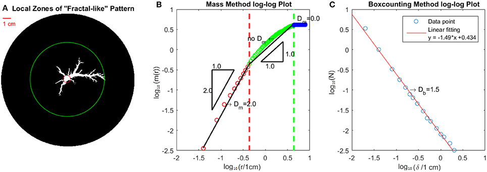
Figure 2. Measurement of fractal dimension from experimentally derived images. (A,B) Show the mass fractal dimension estimation method. In (A), we divide the pattern into 3 zones. The part within the red circle is completely dissolved. Between the red and green circles, “fractal-like” fingers expand in different directions. Outside of the green circle lies an entirely undissolved zone. (B) Shows a log-log plot of mass m(r) vs. radius r, with the colors corresponding to the relevant zones in (A). The black linear solid lines act as a guide for the eye. The slopes of the black lines are illustrated with the triangles. For the red and blue parts, the fractal dimension by mass method D_m is indicated. For the green part, there is no clear linear part, i.e., no well defined mass fractal dimension D_m. In (C) we use the Box-counting Method to obtain the box-counting fractal dimension D_b = 1.5.

From Figure 2, we observe that the Mass Method and the Box-counting Method give very different results. The r² scaling seen in the mass method close to the injection point (r = 0) is caused by the compact structure in this region which goes up to about 0.5 cm from the injection point. Above this length scale the curved green line is due to the decrease in thickness of the fingers but also to the crossover associated to the finite size of the system. The data in Figure 2C, was fitted to a straight line using linear regression with a slope of 1.5 which gives an estimate of a box counting dimension as D_b = 1.5. Notice that there is a small systematic deviation from a linear curve. For the mass within a radius method Figure 2B shows a linear behavior with slope of 2.0 for the region within the red circle in Figure 2A. However in the local zone between the red circle and the green circle in Figure 2A (the green region in Figure 2B), the slope gradually decreases from 2 to 0 and it is not possible to find a unique mass fractal dimension. The black solid line in this region with slope 1 is a reference to the eye. Notice that in the dissolution pattern, the fingers get thinner from the center to the tips. This specific feature of finger width variation found in the dissolution pattern is not found for instance for fractal viscous fingering [28] or DLA structures [29].

5. Experimental Results Compared With Simulations

5.1. Qualitative Comparison

Pictures of the dynamic process of dispersion were taken every 30 s from the beginning of injection until the tracer fluid reached the edge of the sample. The whole process takes 50 min in total, which corresponds to 100 digital images. The experiments are reproducible and the repeated experiments give similar results. Here we present one set of experimental results and data analysis. Results from another experiment is shown in the supplemental data. In Figure 3, four pairs of images corresponding to different time periods are compared between the simulations and the experiment.

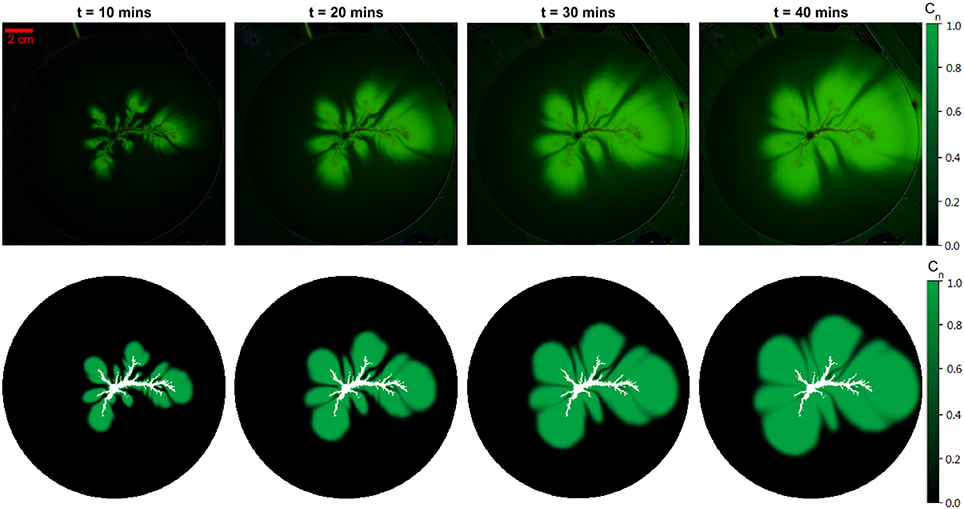
Figure 3. Experimental results compared with simulation images. (Top) Experimental images subtracted by the initial state image. (Bottom) Simulation output of the dissolution pattern. The boundary conditions are extracted from the experimental image before fluid flow begins. The green intensity represents the normalized tracer concentration C_n in the simulation. The vertical pairs of images show comparison after an injection lasting respectively 10/20/30/40 min, which gives a qualitative description of the similarity between the experiments and simulations.

A visual overview of the concentration pattern evolution over time is illustrated in Figure 4. It is constructed by firstly thresholding each grayscale image at I/I_max > 0.2, next computing the incremental difference by subtracting successive thresholded images, and subsequently compositing each of the incremental changes together, leading to Figure 4. This spatiotemporal diagram allows for a more detailed comparison of the dynamic process between simulation and experiment. In the Supplemental Data, Figure S2 shows a similar diagram for another experiment. The simulation and the experimental images look qualitatively very similar to each other.

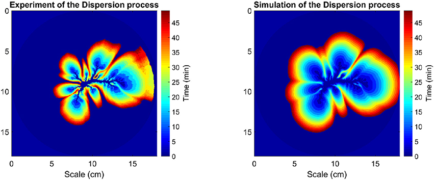
Figure 4. Dynamic process of dispersion with time evolution, time duration 50 min. (Left) Data derived from experimental images; (Right) Equivalent data obtained from numerical simulation.

5.2. Overlap Ratio

To compare quantitatively the experiments and the simulations we have calculated the overlap between two corresponding images with the same size and spatial resolution. We have only considered the overlap within the area of interest, which is the area ${{A}}_D$ defined as the union of area between the experimental and simulations images with a detectable fluorescein concentration. To calculate the overlap we will introduce the overlap ratio (γ_OL) defined as:

where E and S are respectively the experimental and the simulation image (i.e., grayscale fields) which have been normalized (i.e., from 0 to 1), and max(E(i, j), S(i, j)) gives the maximum value of E(i, j) and S(i, j). In the case where E and S are binarized (black and white images), this calculation of the overlap ratio leads to the measure of the ratio of the area of intersection between E and S divided by the area of union between E and S (i.e., A(E∩S)/A(E∪S)), which we call the structure overlap ratio γ_SOL. This computation can also be performed on the gray-scaled images of E and S to obtain the intensity overlap ratio γ_IOL.

In Figure 5, we show a pair of images, E and S, from one experiment and simulation, and the subtracted image ∥E(i, j)−S(i, j)∥. The overlap ratio, indicated in the figure, demonstrates a good similarity between experiment and simulation. From Figure 5, we further observe that the fan-shaped dispersion fingers in the simulation grow somewhat more uniformly than in the experiments. On the other hand the experiment presents longer fingers, but with a more gradual change in the concentration toward the tips. One reason for this difference is that in the simulations the dissolution patterns are taken to be completely dissolved while in the experiments the plaster sample is gradually dissolved. Therefore in the experiments there is a change in the thickness in the dissolved part which we don't consider in the simulations. For a similar reason the assumed undissolved part in the simulations might have some dissolved fingers that we are not able to see in the experiments due to limited resolution. These slightly dissolved fingers will give finer scale structures in the dissolution patterns. Another difference between the experiments and the simulations is that experimentally, a very small fraction of fluid infiltrates into the porous matrix instead of flowing in the open fracture. Flow in the porous medium is however not included in the simulations. Eventually, because the Hele Shaw cell is three dimensional, we expect a concentration distribution in the vertical direction and a gradient in the measured average concentration (averaged in vertical direction). However our simulation is 2D and a gradient in the average concentration due to the 3D velocity field is not considered.

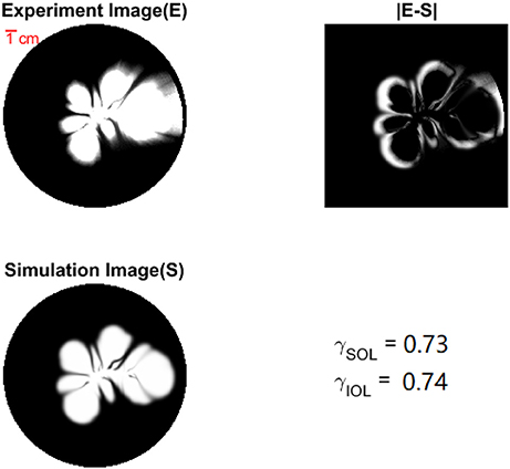
Figure 5. Experimental image (E) and simulation image (S) are resized gray-scaled images from original RGB images. |E − S| displays the intensity difference between experiment and simulation. γ_SOL is the structure overlap ratio which compares the black-white images of E and S. γ_IOL is the intensity overlap ratio comparing E and S which are gray-scaled images.

Figure 6 shows the time dependence of the overlap ratio both for the structure (black-white images) γ_SOL and for the intensity (gray-scaled images) γ_IOL. The overlap ratio increases with time and gets almost stable with an overlap of about 0.7 after injection of 20 min but decreases slightly toward the end, certainly because of the boundary effect in the experiments different from those in the simulations, the experimental plaster sample is not a perfectly circular disk. We implement 3 different simulations to compare with the experimental results, one simulation without diffusion, one with molecular diffusion and one with Taylor dispersion. The figures presented here demonstrate that the simulation with only a convection term is able to roughly simulate what we have observed in the experiments. However, the simulation with diffusion terms (molecular or Taylor dispersion) is more consistent with the experiments than without diffusion terms. The simulations with pure molecular diffusion and Taylor dispersion show almost no significant difference, then the simulation results in the remainder of this paper use 2D model with molecular diffusion.

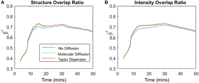
Figure 6. Dynamic process of dispersion: the value of the overlap ratio evolves with time. Total time duration is 50 mins. (A) Shows the structure overlap ratio (derived from black and white images) evolution with time and (B) shows the intensity overlap ratio (derived from grayscale images) evolution with time. Blue lines show the comparison between experimental results and simulation with no diffusion, green lines with molecular diffusion and red lines with Taylor dispersion.

5.3. Concentration Distribution

From the dispersion pictures of both the experiments and the simulations, we clearly observe that the tracer flow acts very differently from what we expect from a point injection or injection from a circular region. These differences are expected on small length scales but are less obvious on large length and time scales. Such differences might be important to bear in mind and evaluate when simple model geometries are used to model transport around wells in large-scale applications. In this section we will compare experimentally and by computer simulations the dispersion in an open fracture with an initial state of a ramified dissolution pattern with simulations with an initial stage of circular injection. We will choose a radius of the circular disk injection $R_d=\sqrt{A/\pi }$ where A is the area of the initial ramified dissolution pattern.

5.3.1. Concentration Distribution Width

A quantitative comparison between the dispersion with a ramified and a circular initial structure was performed by comparing the mean value and standard deviation of the tracer concentration on circles of different radii r. Figure 7 illustrates the difference in the tracer concentration distribution on a circle of a certain radius (here r = 3.4 cm) between the initial circular front and the ramified front. The mean value of the normalized tracer concentration on a circle is defined as

where N(r) is the number of pixels along the circle with radius r and C_n(r_i) is the normalized tracer concentration at position r_i. Let σ(r) be the standard deviation of C_n(r) on the circle for a fixed value of r. Figure 8 shows the mean value < C_n(r)> and the standard deviation σ(r) at different radii r among experimental images and simulations with circular and ramified initial fronts. The Figure 8 clearly demonstrates that the simulation with a ramified initial front fits the experiment much better than the simulation with a flat circular initial front. In the standard deviation Figure 8B, a small peak is observed in the circular front simulation (green line) which is not expected from the analytical results. This peak is caused by pixel-size deviations due to a finite pixel resolution describing the circle.

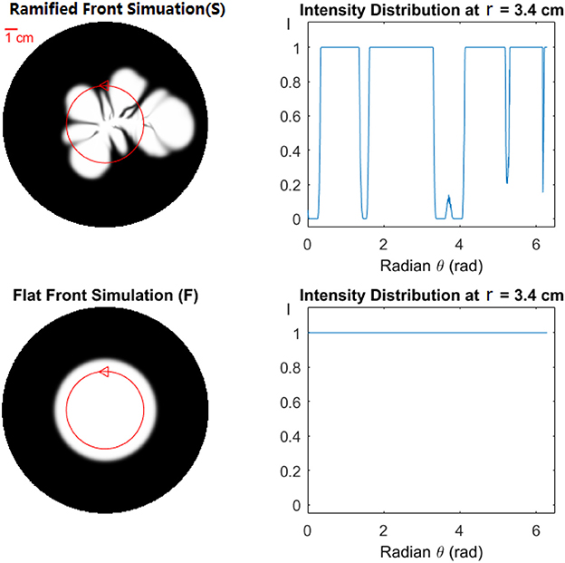
Figure 7. Effect of front geometry. (Top) Ramified Front Simulation (S) shows the result of simulation with the ramified front (dissolution pattern). (Bottom) Flat Front Simulation (F). The normalized intensity distribution at r = 3.4 cm, marked with a red circle on the left, is shown as a function of angle on the right. The distribution begins at the marked triangle, and continues counter-clockwise.

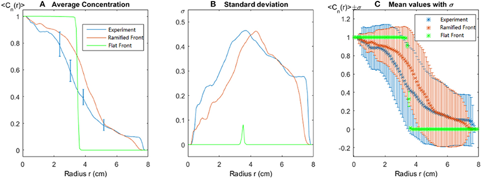
Figure 8. Spatial dependence of structure as function of the circle radius. (A) The normalized average concentration, the error bar comes from experimental measurement for fluid tracer concentration according to the calibration performed in Supplemental Data. (B) Its standard deviation and (C) mean values with error bars at one standard deviation. In all cases, the blue line is the experimental result, the red line corresponds to the simulation with an injection ramified front corresponding to the dissolution pattern present in this experiment, and the green line represents the simulation result with an internal flat (circular) front of similar area.

We will define the width Δr(t) of the normalized mean concentration distribution as the difference in radius between < C_n(r) >= 0.8 and < C_n(r) >= 0.2 as illustrated in Figure 9A. For the circular initial front simulation (yellow line in Figure 9C), Δr(t) stays stable at a low level, and the fluctuation in the curve is due to few data points. While the circular initial front simulation is completely different from the experimental curve, the simulation with the ramified initial front is much closer to the experimental results. The width of the mean concentration distribution Δr(t) in both the experiments and the simulation with ramified initial front increases to a peak and then decreases to a stable value.

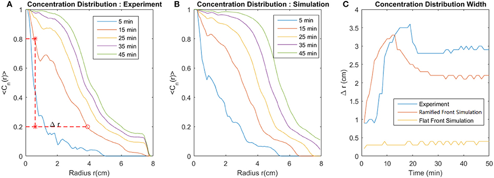
Figure 9. Evolution of the average concentration distribution at different times. (A) Experimental data. (B) Simulation data. The red dotted line in (A) shows how we get the width of concentration distribution at 15 min (Δr(t = 25min)) which is the distance between the red circle (20% of reference concentration) and red asterisk (80% of reference concentration). (C) Displays the width of concentration distribution evolution with time, the blue line is the experimental result, the red line is the simulation with an injection ramified front identical to the dissolution pattern present in this experiment, and the yellow one is the simulation result with a flat circular front of similar area.

From Figures 9A,B, we observe a noticeable change of the concentration distribution from a wider distribution at a time t = 10–15 min to a more localized front at later times t > 20 min. In the Supplemental Data Figure S3, another experiment reproduces a similar mean concentration distribution. At short times the angle average concentration curves < C_n(r)> are dominated by the ramified fractal-like initial structure, but they change to a very different behavior at large scales, to get dominated by the complex velocity field generated by the same ramified dissolution structure and diffusion. On average < C_n(r)> has a well defined width at large times, but it is much wider than what one would expect from a circular initial front, 5 times wider for simulation and 7 times wider for experiment. For a constant radius r there are large fluctuations in the local values of C_n(r) at different directions. These fluctuations in the concentration are due to velocity fluctuations in the initial ramified structure (see Figure 7). An interesting and open question is if these fluctuations will be reduced or disappear for a sufficient large systems and times. Will the model with a circular initial state describe the system at large length scales and times? In the next section, we will propose a theoretical calculation to address this question.

5.3.2. Concentration Distribution Shape

A key question is whether the anisotropy of the concentration profiles will survive over arbitrarily large distances from the dissolution structure. In order to address this question we first pose the same question for the flow field u: Will u remain anisotropic indefinitely? One way to answer this is to consider a group of two point sources of equal pressure and extent rather than the complex dissolution structure. In this way the distance over which an anisotropic flow field becomes isotropic or not may be explored. Taking the two sources to be located at ±r₁ where r₁ is the characteristic radius of the dissolution structure, we may work out the pressure field and by Darcy's law, the flow field.

We will take the pressure, or rather the overpressure relative to the atmospheric pressure, to satisfy the 2D Laplace equation, take on the value P₀ inside a radius a around ±r₁ and vanish at some large distance R. This pressure may to a good approximation be written as

The approximation consists in the fact that the point where the pressure vanishes is shifted a small distance of the order r₁. Darcy's law now gives the Darcy velocity

where the unit vector e_r = r/r and the higher order term depends on products like e_r · r₁. This result shows that the flow velocity field becomes isotropic over a distance of the order r₁. We define this distance of the order r₁ for our experimental geometry as r₀, which in our experiments, r₀ is the length of the longest dissolution finger. The argument is that the the two point sources must create a flow field that is at least as anisotropic as the real field, or worse. Since the model field decays to the isotropic field as ${(r_1/r)}^2$, we conclude that the real field decays as quickly, or quicker.

Now, the fact that the velocity becomes isotropic does not imply that the concentration field does, as this field is governed by an anisotropic source. We calculate the skin-depth to go as the diffusion length $l_D=\sqrt{2D_{\perp }t}$ where D_⊥ is a transverse dispersion constant. This constant characterizes the porous media. In this case, since this medium is just a gap of width h, we may take D_⊥ ≈ D_m. Close to the injection point anyhow, once it is at a point within a few skin-depths of the injection points, it should have reached a concentration which is equal to the imposed central concentration, at least due to diffusion if this did not happen in the first place by convection because the point considered was along a fast transporting finger. So we expect a zone growing like $\sqrt{D_{\perp }t}$ where the concentration is homogeneous and naturally isotropic but outside of this zone, possible anisotropy is discussed by calculating the convection length l_C. The convection length is defined as the concentration profile convection length outside the circle of r₀, l_C = ∫udt so that

or $d{l}_c^2=\frac{Q}{\pi h}dt$, which immediately gives

Here the time t starts from t_D where t_D is the time it takes for molecular diffusion alone to homogenize the immediate neighborhood of the dissolved cluster. Now we take the maximum convection length l_max and the minimum convection length l_min into account, the maximum convection length l_max starts growing outside of the circle of r₀ while the minimum convection length l_min starts growing after t_D. So the ratio of these two convection lengths is:

The length difference of l_max and l_min is:

From the calculations above, we conclude that the ratio between the maximum and the minimum convection length tends to 1 and the length difference between two decreases as t^−1/2 and tends to 0. It implies that the anisotropy of the concentration profiles will vanish after an enough long time. To see an isotropic behavior, a theoretical criterion for a length scale can be calculated from Equations (10, 11) requiring t_D/t less than a small number. For instance, t_D/t < 0.1 and $\sqrt{2D_m{t}_D}=d_D$ where d_D is a distance between dispersion fans that could be estimated from Figure 3 as d_D = 0.5 cm. Consequently, the length scale $l=\sqrt{10}\sqrt{\frac{Q{t}_D}{\pi h}}=\sqrt{\frac{5Q}{\pi D_{m}h}}·d_D$ to see an isotropic behavior will be of the order of 1m. These theoretical conclusions are also verified by the simulation results. The simulation is implemented with the same system of initial dissolution pattern but expanding by scale of 8 times so that we can observe the concentration profile after a long time, see Figure 10.

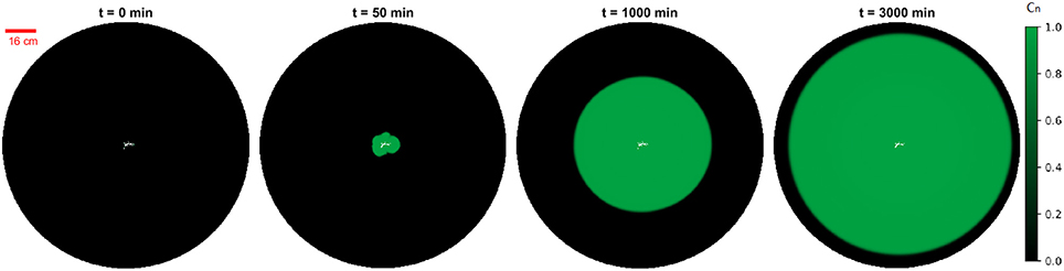
Figure 10. Example of persistence of anisotropy at larger length scales. The simulation images are obtained from the molecular diffusion model, with the same dissolution pattern as before but the whole system is expanded by scale of 8 times. The green intensity represents the normalized tracer concentration C_n in the simulation. The images show the concentration profile after an injection lasting respectively 0/50/1, 000/3, 000 min. We observe that the anisotropy of the concentration profile vanishes gradually with time.

The convection lengths are obtained by calculation of the distance between the points at the boundary of the dispersion pattern and the center of the circular system from the simulation data. We analyze the maximum and minimum convection length evolution with time, the ratio and the difference between the two lengths. The results are shown in Figure 11.

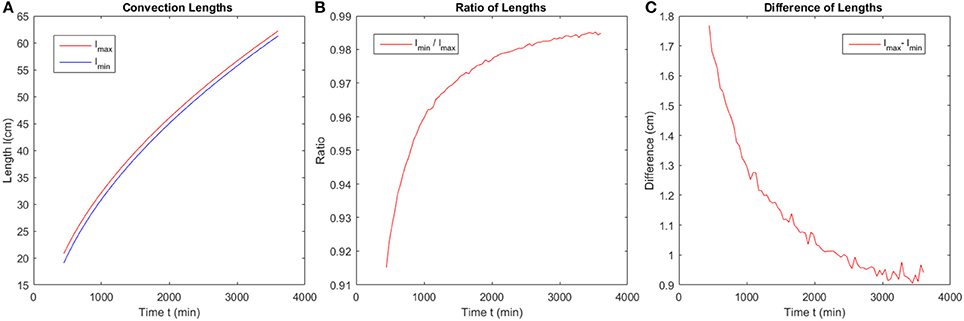
Figure 11. Evolution of characteristic length scales in the system with time. (A) The maximum and minimum convection length evolution with time. (B) The ratio of the two lengths shown in (A), which approaches unity at long times. (C) The difference of the two lengths shown in (A), which approaches zero at long times.

From the simulation results shown in Figure 12, we make a log-log plot of the data curve and compare it with theoretical calculations. The convection length follows the relation $l_c\propto t^{1/2}$. The ratio of lengths tends to 1 and the difference between lengths has a decreasing trend. The fluctuations of the simulation data is because the boundary line of concentration profile is not a prefect line numerically and also the center is not a prefect point. For the initial state which is close to the inlet with ramified dissolution pattern, the velocity field is not radial flow. For the late stage which is close to the finite edge of system, the boundary effect will influence the concentration profile close to the rim. The deviations between the simulation results and theoretical calculation under these two limiting conditions are expected as we observe in Figure 12.

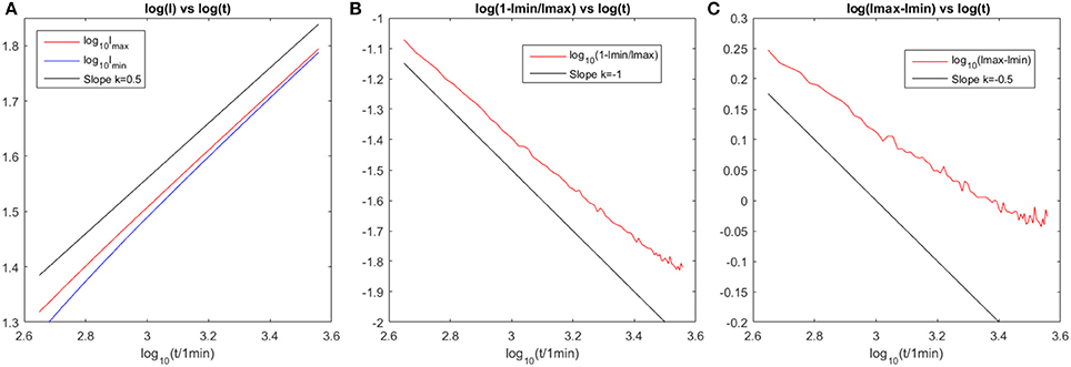
Figure 12. Evolution of characteristic length scales in the system with time. The corresponding log-log plot for Figure 11 is shown. (A) Logarithmic plot of the maximum and minimum convection length evolution with time, where the black line gives a reference slope of k = 0.5 which implies that the curves tend to follow the power law of $\sqrt{t}$. (B) One minus the ratio of the two lengths evolution with time follows the power law of 1/t with a reference slope k = −1. (C) The difference of the two lengths evolution with time follows the power law of $1/\sqrt{t}$ with a reference slope k = −0.5.

Using a similar development, in the case of injection in a three dimensional porous medium from a ramified structure, without large scale correlations in the permeability, one expects at large scale, the flow velocity in a radial field $u(l_c)=Q/(4\pi l_c^2)$ and the convection length $l_c={(3Qt/(4\pi ))}^{1/3}$. A concentration field converging at large times to the point source solution, with a ratio of minimum convection length over the maximum one,

and a difference

In this 3D case, we predict that the anisotropic concentration patterns would eventually always go away, the maximum and minimum convection length ratio and difference would follow the power law as a function of t as shown in the calculation above.

6. Conclusion

We have performed experiments and computer simulations of dispersion in an open fracture with an initial state emerging from a ramified dissolution pattern. A fluorescent technique was used to measure the tracer concentration in a transparent Hele Shaw cell. We implemented a 2D simulation which in addition to convective motion can include both molecular diffusion and Taylor diffusion. For the investigated patterns, simulations with molecular diffusion and Taylor diffusion have no significant difference. The ramified dissolution structures have a significant effect on the local concentration C_n(r) and the concentration averaged over angles <C_n(r)> both for small and large length and time scales. The shape of the concentration distributions far from the dissolution structure is discussed with some theoretical calculations. The convergence in open systems of structures injected from ramified patterns to the point-like (or circular) injection solution is not obvious: When molecular diffusion presents a skin depth $\sqrt{2Dt}$ exceeding largely the central zone size R_d, the concentration gradients in the central zone are expected to reduce, and the concentration field should be smoother there. Nonetheless, the strong anisotropy of the permeability in the central region leads to clear fingering outside this region. Whether the influence of these fingers is felt only up to a finite range is questionable, in particular in this radial geometry, since the center of the different emerging fingers diverges with time. We make some theoretical calculations and simulations to conclude that the anisotropy of the concentration distribution in the system will vanish at sufficiently large length and time scales. The experimental verification of isotropy of the tracer concentration at large scales is an interesting question for further experimental work. From the theoretical calculation and our simulation result we estimate that we need an experimental model of the order of 1m to reach this isotropy. At the expected 3D structure, we predict that the shape of concentration distribution far from the dissolution structure will eventually experience a slowly vanishing anisotropy, in future work it would certainly be nice to explore these 3D structures both experimentally and numerically to see how they correspond to these predictions.

Author Contributions

LX and KM designed the experiment. LX performed the experiments, analyzed the data and authored the paper. BM conducted the simulations. EF contributed to the idea for the simulations and performed some theoretical calculations together with RT and KM. RT, EF, and KM assisted with the interpretation and data analysis, and editing of the manuscript.

Conflict of Interest Statement

The authors declare that the research was conducted in the absence of any commercial or financial relationships that could be construed as a potential conflict of interest.

Acknowledgments

This project has received funding from the European Union's Seventh Framework Programme for research, technological development and demonstration under grant agreement no 316889. We acknowledge the support of the University of Oslo and the support by the Research Council of Norway through its Centres of Excellence funding scheme, project number 262644, and the INSU ALEAS program. We thank Mihailo Jankov for technical support and Marcel Moura, Fredrik K. Eriksen, Monem Ayaz, and Guillaume Dumazer for useful discussions.

Supplementary Material

The Supplementary Material for this article can be found online at: https://www.frontiersin.org/articles/10.3389/fphy.2018.00029/full#supplementary-material

References

1. Taylor G. Dispersion of soluble matter in solvent flowing slowly through a tube. Proc R Soc Lond A Math Phys Eng Sci. (1953) 219:186–203. doi: 10.1098/rspa.1953.0139
2. Tang D, Frind E, Sudicky EA. Contaminant transport in fractured porous media: analytical solution for a single fracture. Water Resour Res. (1981) 17:555–64. doi: 10.1029/WR017i003p00555
3. Sudicky E, Frind E. Contaminant transport in fractured porous media: analytical solutions for a system of parallel fractures. Water Resour Res. (1982) 18:1634–42. doi: 10.1029/WR018i006p01634
4. Boschan, A, Auradou, H, Ippolito, I, Chertcoff, R, and Hulin, JP Miscible displacement fronts of shear thinning fluids inside rough fractures. Water Resour Res. (2007) 43:W03438. doi: 10.1029/2006WR005324
5. Sané J, Padding JT, Louis AA. Taylor dispersion of colloidal particles in narrow channels. Mol Phys. (2015) 113:2538–45. doi: 10.1080/00268976.2015.1035768
6. Måloy KJ, Feder J, Boger F, Jossang T. Fractal structure of hydrodynamic dispersion in porous media. Phys Rev Lett. (1988) 61:2925. doi: 10.1103/PhysRevLett.61.2925
7. Ippolito I, Hinch E, Daccord G, Hulin J. Tracer dispersion in 2-d fractures with flat and rough walls in a radial flow geometry. Phys Fluids A Fluid Dyn. (1993) 5:1952–62. doi: 10.1063/1.858822
8. Alencar AM, Andrade JS, Lucena LS. Self-organized percolation. Phys Rev E (1997) 56:R2379. doi: 10.1103/PhysRevE.56.R2379
9. Andrade JS Jr, Costa UMS, Almeida MP, Makse HA, Stanley HE. Inertial effects on fluid flow through disordered porous media. Phys Rev Lett. (1999) 82:5249. doi: 10.1103/PhysRevLett.82.5249
10. Parteli EJR, da Silva LR, Andrade JS Jr. Self-organized percolation in multi-layered structures. J Stat Mech Theory Exp. (2010) 2010:P03026. doi: 10.1088/1742-5468/2010/03/p03026
11. Bodin J, Delay F, De Marsily G. Solute transport in a single fracture with negligible matrix permeability: 1. Fundamental mechanisms. Hydrogeol J. (2003) 11:418–33. doi: 10.1007/s10040-003-0268-2
12. Qian J, Zhan H, Zhao W, Sun F. Experimental study of turbulent unconfined groundwater flow in a single fracture. J Hydrol. (2005) 311:134–42. doi: 10.1016/j.jhydrol.2005.01.013
13. Koyama T, Neretnieks I, Jing L. A numerical study on differences in using navier–stokes and reynolds equations for modeling the fluid flow and particle transport in single rock fractures with shear. Int J Rock Mech Mining Sci. (2008) 45:1082–101. doi: 10.1016/j.ijrmms.2007.11.006
14. Bauget F, Fourar M. Non-fickian dispersion in a single fracture. J Cont Hydrol. (2008) 100:137–48. doi: 10.1016/j.jconhyd.2008.06.005
15. Rastiello G, Boulay C, Dal Pont S, Tailhan JL, Rossi P. Real-time water permeability evolution of a localized crack in concrete under loading. Cement Concrete Res. (2014) 56:20–8. doi: 10.1016/j.cemconres.2013.09.010
16. Daccord G, Lenormand R. Fractal patterns from chemical dissolution. Nature (1987) 325:41–3. doi: 10.1038/325041a0
17. Fredd CN, Fogler HS. Influence of transport and reaction on wormhole formation in porous media. AIChE J. (1998) 44:1933–49. doi: 10.1002/aic.690440902
18. Szymczak P, Ladd AJC. Instabilities in the dissolution of a porous matrix. Geophys Res Lett. (2011) 38:L07403. doi: 10.1029/2011GL046720
20. Szymczak P, Ladd AJC. Wormhole formation in dissolving fractures. J Geophys Res Solid Earth (2009) 114:B0620. doi: 10.1029/2008JB006122
21. Daccord G. Chemical dissolution of a porous medium by a reactive fluid. Phys Rev Lett. (1987) 58:479. doi: 10.1103/PhysRevLett.58.479
22. Wang H, Bernabé Y, Mok U, Evans B. Localized reactive flow in carbonate rocks: core-flood experiments and network simulations. J Geophys Res Solid Earth (2016) 121:7965–83. doi: 10.1002/2016JB013304
23. Culbertson CT, Jacobson SC, Ramsey JM. Diffusion coefficient measurements in microfluidic devices. Talanta (2002) 56:365–73. doi: 10.1016/S0039-9140(01)00602-6
24. Walker D. A fluorescence technique for measurement of concentration in mixing liquids. J Phys E Sci Instrum. (1987) 20:217. doi: 10.1088/0022-3735/20/2/019
25. Aris R. On the dispersion of a solute in a fluid flowing through a tube. Proc R Soc Lond A Math Phys Eng Sci. (1956) 235:67–77.
26. Boschan A, Charette V, Gabbanelli S, Ippolito I, Chertcoff R. Tracer dispersion of non-newtonian fluids in a hele–shaw cell. Phys A Stat Mech Appl. (2003) 327:49–53. doi: 10.1016/S0378-4371(03)00437-0
27. Kurganov A, Tadmor E. New high-resolution central schemes for nonlinear conservation laws and convection–diffusion equations. J Comput Phys. (2000) 160:241–82. doi: 10.1006/jcph.2000.6459
28. Måløy KJ, Feder J, Jøssang T. Viscous fingering fractals in porous media. Phys Rev Lett. (1985) 55:2688. doi: 10.1103/PhysRevLett.55.2688
29. Witten TA, Sander LM. Diffusion-limited aggregation. Phys Rev B (1983) 27:5686. doi: 10.1103/PhysRevB.27.5686
30. Barabási AL, Stanley HE. Fractal Concepts in Surface Growth. Cambridge: University Press (1995).
Keywords: dispersion, fracture, convection-diffusion, fractal-like, Hele-Shaw cell, fluorescein tracer
Citation: Xu L, Marks B, Toussaint R, Flekkøy EG and Måløy KJ (2018) Dispersion in Fractures With Ramified Dissolution Patterns. Front. Phys. 6:29. doi: 10.3389/fphy.2018.00029
Received: 29 January 2018; Accepted: 23 March 2018;
Published: 16 April 2018.
Edited by:
José S. Andrade Jr., Federal University of Ceará, BrazilReviewed by:
Eric Josef Ribeiro Parteli, Universität zu Köln, GermanyRamon Castañeda-Priego, Universidad de Guanajuato, Mexico
Copyright © 2018 Xu, Marks, Toussaint, Flekkøy and Måløy. This is an open-access article distributed under the terms of the Creative Commons Attribution License (CC BY). The use, distribution or reproduction in other forums is permitted, provided the original author(s) and the copyright owner are credited and that the original publication in this journal is cited, in accordance with accepted academic practice. No use, distribution or reproduction is permitted which does not comply with these terms.
*Correspondence: Le Xu, le.xu@fys.uio.no