Robust stability at the Swallowtail singularity

1. Introduction. Ziegler-Bottema Destabilization Phenomenon

In 1956, motivated by the paradoxical effect of dissipation on the threshold of oscillatory instability of mechanical structures under non-conservative loadings [1], Bottema [2] studied the domain of asymptotic stability¹ of a fourth-order real polynomial

He observed that the necessary and sufficient conditions

for the polynomial to be Hurwitz, i.e., to have all its roots in the left half of the complex plane, are not changed by the transformation μ = cλ, where $c=\sqrt[4]{b_4}>0$. Indeed, after denoting

the inequalities (2) are equivalent to the conditions

that are necessary and sufficient for the polynomial

to be Hurwitz. The domain (4) was plotted by Bottema in the (a₁, a₃, a₂)-space; see Figure 1.

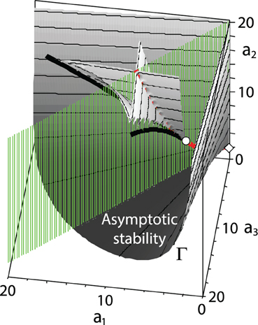
Figure 1. A singular boundary Γ of the domain of asymptotic stability (4) of the polynomial (5) with the Whitney umbrella singularity at the point (a₁, a₃, a₂) = (0, 0, 2), marked by the diamond symbol. Inside the domain of asymptotic stability a part of the discriminant surface of the polynomial is situated with the Swallowtail singularity at the point (4, 4, 6) marked as an open circle. Inside the spike bounded by the discriminant surface all the roots of the polynomial (5) are real and negative. The green planar sector is the tangent cone (10) to the domain of asymptotic stability at the Whitney umbrella singularity.

Bottema realized that the boundary Γ of the asymptotic stability domain (4) is a ruled surface² generated by straight lines a₃ = ra₁, a₂ = r + 1/r, where r ∈ (0, ∞). The boundary Γ has a self-intersection along the ray a₂ ≥ 0 of the a₂-axis. Two generators pass through each point of the ray; they coincide at a₂ = 2 (r = 1), and for a₂ → ∞ their directions tend to those of the a₁- and a₃-axis (r = 0, r = ∞). Remarkably [2, 3], the point (a₁, a₃, a₂) = (0, 0, 2) is on Γ, but if one tends to the a₂-axis along the line a₃ = ra₁ the coordinate a₂ has the limit r + 1/r > 2 except for r = 1, when a₂ = 2. The point (0, 0, 2) marked by the diamond symbol in Figure 1 is the Whitney umbrella singularity [4]. The surface defined by the equation

is just another representation of a standard crosscap surface f_std(u, v) = (u, uv, v²): ℝ² → ℝ³, which also bears the name of the Whitney umbrella [5].

For given a₁ = a_{1, 0} and a₂ = a_{2, 0} > 2, exactly two points correspond at the crosscap (6) with the third coordinate determined from the equation

where each sign is associated with one of the two sheets of the crosscap that intersect along the interval a₂ ≥ 2; see Figure 1. Writing the equations for the tangent planes at these points

we find that approaching the singular point (0, 0, 2) along the a₂-axis, i.e., assuming a_{1, 0} = 0 in (8) and then letting a_{2, 0} tend to 2, results in the collapse of the two planes into one defined by the equality

The limit (9) of the tangent planes is the tangent cone to the crosscap at the Whitney umbrella singularity [5]. A part of the plane (9) that lies inside the domain of asymptotic stability (4) constitutes a set of all directions leading from the point (0, 0, 2) to the stability region

The tangent cone (10) to the domain of asymptotic stability at the Whitney umbrella singularity, which is shown in green in Figure 1, is degenerate in the (a₁, a₃, a₂)-space because it selects a set of measure zero on a unit sphere with the center at the singular point [6–8].

In 1971, Arnold [4] considered parametric families of real matrices and studied which singularities on the boundary of the asymptotic stability domain in the space of parameters are not destroyed by small perturbation of the family, i.e., are structurally stable or generic singularities. He composed a list of generic singularities in parameter spaces of low dimension which revealed, in particular, that the Whitney umbrella persists on the stability boundary of a real matrix of arbitrary dimension if the number of parameters is not less than three, i.e., the singularity is of codimension 3.

The singular point (a₁, a₃, a₂) = (0, 0, 2) corresponds to a double complex conjugate pair of roots λ = ±i of the polynomial (5).

At the line of self-intersection of the Whitney umbrella formed by the ray a₂ > 2 of the a₂-axis there are two distinct complex conjugate pairs of imaginary roots [2] indicating Lyapunov (marginal) stability. However, the threshold of stability a₂ = 2 is extremely sensitive to the coefficients a₁ and a₃ as is seen from (6).

Indeed, fix â₁ ≠ â₂ and let a₁ = εâ₁ and a₃ = εâ₃ (where 0 < ε« 1). Then, using (6), we find that the increment to the critical value of the coefficient a₂ is

In other words, the stability threshold acquires a finite increment Δa₂ > 0 even if the perturbation of the coefficients a₁ and a₃ is infinitesimally small for almost all combinations of a₁ and a₃, except in the case a₁ = a₃. The minimal threshold of marginal stability a₂ = 2 at a₁ = 0 and a₃ = 0 corresponding to the double imaginary root is thus structurally unstable: generic combinations of the parameters a₁ and a₃ at a₂ = 2 lie in the domain of instability [1–3, 9]. Therefore, looking for extremal values of a parameter (a₂ in our case) at the boundary of asymptotic stability may lead to structurally unstable stability thresholds at the singular points of the stability boundary corresponding to multiple roots.

The more basic fact that multiple roots of a polynomial are sensitive to perturbation of the coefficients is a phenomenon that was studied already by Isaac Newton, who introduced the so-called Newton polygon to determine the leading terms of the perturbed roots as fractional powers of a perturbation parameter. It follows that, in matrix analysis, eigenvalues are in general not locally Lipschitz at points in matrix space with non-semi-simple eigenvalues³ [10–13], and, in the context of dissipatively perturbed Hamiltonian systems, [9, 14, 15]. Thus, it has been well-understood for a long time that perturbation of multiple roots or multiple eigenvalues on or near the stability boundary is likely to lead to instability⁴.

Because of the sensitivity of multiple roots and eigenvalues to perturbation, in engineering and control-theoretical applications a natural desire is to “cut the singularities off” by constructing convex inner approximations to the domain of asymptotic stability [17, 18]. Nevertheless, multiple roots per se are not undesirable. Indeed, multiple roots also occur deep inside the domain of asymptotic stability. Although it might seem paradoxical at first sight, such configurations are actually obtained by minimizing the so-called polynomial abscissa in an effort to make the asymptotic stability of a linear system more robust, as we now explain.

2. Abscissa Minimization and Multiple Roots

The abscissa⁵ of a polynomial p is the maximal real part of its roots:

We restrict our attention to monic polynomials with real coefficients and fixed degree n: since these have n free coefficients, this space is isomorphic to ℝⁿ. On this space, the abscissa is a continuous but non-smooth, in fact non-Lipschitz, as well as non-convex, function whose variational properties have been extensively studied using non-smooth variational analysis [21–24].

Now set n = 4, consider the set of polynomials p(λ) defined in (5), and consider the restricted set of coefficients

For these coefficients, the abscissa a(p) is shown as a function of a₁ by the bold red curve in Figure 2. The roots are

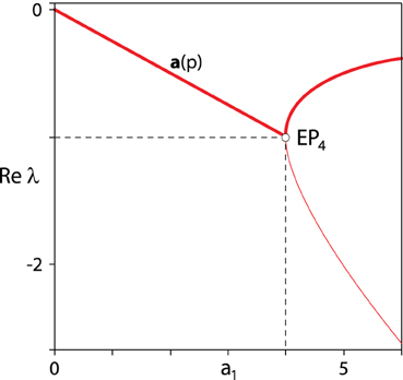
Figure 2. The real parts of the roots of the polynomial (5) with the coefficients in the set (13) and (shown by the bold red curve) the abscissa (12).

When 0 ≤ a₁ < 4 (a₁ > 4), the roots λ_{1, 2} and λ_{3, 4} are complex (real) with each pair being double, that is with multiplicity two. At a₁ = 4 there is a quadruple real eigenvalue −1. So, we refer to the set (13) as a set of exceptional points⁶ (abbreviated as the EP-set).

When a₁ > 0, the EP-set (13) (shown by the red curve in Figure 3) lies within the tangent cone (10) to the domain of asymptotic stability at the Whitney umbrella singularity (0, 0, 2). The points in the EP-set all define polynomials with two double roots (denoted EP₂) except (a₁, a₃, a₂) = (4, 4, 6), at which p has a quadruple root and is denoted EP₄; see Figure 3.

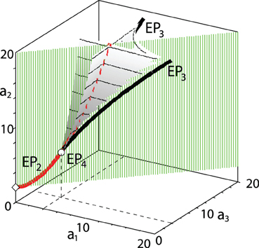
Figure 3. The discriminant surface (gray) and the tangent cone (green) to the domain of asymptotic stability. Inside the tangent cone (10) the red curve marks the EP-set (13). The part of the EP-set above the Swallowtail singularity at the point (4, 4, 6) forms a line of self-intersection of the discriminant surface. The bold black curves are cuspidal edges of the discriminant surface corresponding to triple negative real roots.

Let us consider how the roots move in the complex plane when a₁ and a₃ coincide and are set to specific values and a₂ increases from zero, as shown by black curves in Figure 4. When a₁ = a₃ < 4, the roots that initially have positive real parts and thus correspond to unstable solutions move along the unit circle to the left, cross the imaginary axis at a₂ = 2 and merge with another complex conjugate pair of roots at a₂ = 2 + a²₁/4, i.e., at the EP-set. Further increase in a₂ leads to the splitting of the double eigenvalues, with one conjugate pair of roots moving back toward the imaginary axis. By also considering the case a₁ = a₃ > 4, it is clear that when a₁ and a₃ coincide, the choice a₂ = 2 + a²₁/4 minimizes the abscissa, with the polynomial p on the EP-set, see Figure 5. Furthermore, when a₁ = a₃ is increased toward 4 from below, the coalescence points (EP₂) move around the unit circle to the left. This conjugate pair of coalescence points merges into the quadruple real root λ = −1 (EP₄) when a₁ = a₃ = 4 and hence a₂ = 6, as is visible in Figure 6. If a₁ = a₃ is increased above 4 the quadruple point EP₄ splits again into two exceptional points EP₂, one of them inside the unit circle, Figure 5.

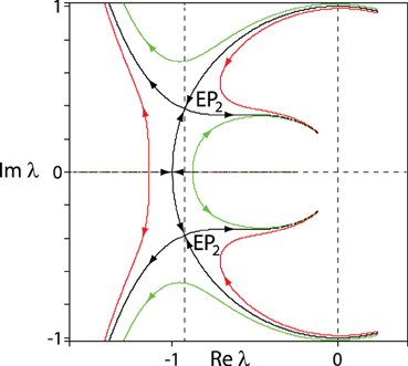
Figure 4. Trajectories of roots of the polynomial (5) when a₂ increases from 0 to 15 and: a₁ = a₃ = 3.7 (black); a₁ = 3.7, a₃ = 3.6 (red); a₁ = 3.6, a₃ = 3.7 (green).

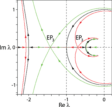
Figure 5. Trajectories of roots of the polynomial (5) when a₂ increases from 0 to 15 and: a₁ = a₃ = 5 (black); a₁ = 5, a₃ ≈ 4.621 (red); a₁ ≈ 4.621, a₃ = 5 (green), indicating that although three roots coalesce into a triple negative real root (EP₃) with Reλ < −1, there is another simple negative real root with Reλ > −1.

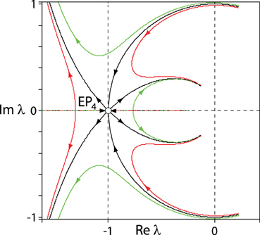
Figure 6. Trajectories of roots of the polynomial (5) when a₂ increases from 0 to 15 and: a₁ = a₃ = 4 (black); a₁ = 4, a₃ = 3.9 (red); a₁ = 3.9, a₃ = 4 (green). The global minimum of the abscissa is attained when all the roots coalesce into the quadruple root λ = −1 (EP₄).

Thus, all indications are that the abscissa is minimized by the parameters corresponding to EP₄, with a quadruple root at −1. In fact, application of the following theorem shows that the abscissa of (5) is globally minimized by the EP₄ parameters.

Theorem [27, Theorems 7 and 14]⁷. Let 𝔽 denote either the real field ℝ or the complex field ℂ. Let b₀, b₁, …, b_n ∈ 𝔽 be given (with b₁, …, b_n not all zero) and consider the following family of monic polynomials of degree n subject to a single affine constraint on the coefficients:

Define the optimization problem

Let

First, suppose 𝔽 = ℝ. Then, the optimization problem (15) has the infimal value

where h⁽ⁱ⁾ is the i-th derivative of h and k = max{j: b_j ≠ 0}. Furthermore, the optimal value a* is attained by a minimizing polynomial p* if and only if −a* is a root of h (as opposed to one of its derivatives), and in this case we can take

Second, suppose 𝔽 = ℂ. Then, the optimization problem (15) always has an optimal solution of the form

with −γ given by a root of h (not its derivatives) with largest real part.

In our case, 𝔽 = ℝ, n = 4 and the affine constraint on the coefficients of p is simply a₄ = 1. So, the polynomial h is given by

Its real root with largest real part is 1, and its derivatives have only the zero root. So, the infimum of the abscissa a over the polynomials (5) is −1, and this is attained by

that is, with the coefficients at the exceptional point EP₄. There is nothing special about n = 4 here; if we replace 4 by n we find that the infimum is still −1 and is attained by p*(λ) = (λ + 1)ⁿ.

3. Swallowtail Singularity as a Global Minimizer of the Abscissa

Let us look at the dynamics of the roots of the polynomial (5) in the complex plane, when a₁ ≠ a₃, i.e., when the variation of a₂ happens at a distance from the tangent cone (10). If a₁ ≤ 4 and a₃ ≤ 4 (as in Figures 4, 6) the complex roots do not coalesce at EP₂ or EP₄ but instead some of them turn back toward the imaginary axis before reaching the unit circle. Such parameter configurations are therefore not optimal. However, when a₁ > 4 or a₃ > 4 other scenarios of the root movement are possible: for example, formation of triple negative real roots as in Figure 5. Note, however, that even when the triple negative real root occurs at Re λ < −1, there is another negative real root inside the unit circle. Therefore, in accordance with the above Theorem, configurations with triple roots are not global minimizers of the abscissa of the polynomial (5). Nevertheless, it is instructive to understand the set in the (a₁, a₃, a₂)-space where the roots of the polynomial are real and negative, but not necessarily simple.

Consider the discriminant⁸ Δ of the polynomial (5) and equate it to zero:

In the (a₁, a₃, a₂)-space, the polynomial (5) has at least one multiple root at the points of the set given by (17). For example, in the plane a₁ = a₃

and the equation Δ = 0 yields the straight line a₂ = 2(a₃ − 1) and parabola a₂ = 2 + a²₃/4 that touch each other at a₃ = 4 and a₂ = 6, which corresponds to the EP₄ point in Figure 3. This corresponds to the quadruple negative real root −1 of the polynomial (5), which is a global minimum of its abscissa.

Plotting the discriminant surface (17), we see in Figure 3 that it has a self-intersection along the part of the EP-set (13) selected by the inequality a₂ ≥ 6 and two cuspidal edges defined in the parametric form as

At the cuspidal edges the polynomial (5) has a triple negative real root and a simple negative real root. For example, at the points $\left(\frac{28}{9}\sqrt{3},4\sqrt{3},10\right)$ and $\left(4\sqrt{3},\frac{28}{9}\sqrt{3},10\right)$ we have, respectively,

At the point EP₄ with the coordinates (4, 4, 6) in the (a₁, a₃, a₂)-space the discriminant surface has the Swallowtail singularity, which is a generic singularity of bifurcation diagrams in three-parameter families of real matrices [19, 28]; see Figure 3.

Therefore, the coefficients of the globally minimizing polynomial (16) are exactly at the Swallowtail singularity of the discriminant surface of the polynomial (5).

We notice, however, that the bifurcation diagram shown in Figure 3 allows us to predict the root configurations that generically exist at the global optimum of the polynomial abscissa when more than one affine constraint restricts the coefficients of the polynomial. Indeed, let the number of affine constraints be κ. Then, according to [28] and [19], the highest possible codimension of a generic singularity in the restricted space of parameters is n − κ. Therefore, introduction of an additional constraint (κ = 2) generically removes the quadruple real root λ = −1 of codimension 3 from the candidates to be global minimizers: n − κ = 2. Assuming for example a₂ = const., we find only double real or complex conjugate roots when 0 < a₂ < 6 whereas when a₂ > 6 we find only triple real roots. As Figure 7 shows, when a₂ is restricted to 10, the global minimum is at the algebraically smallest of the triple negative roots (18).

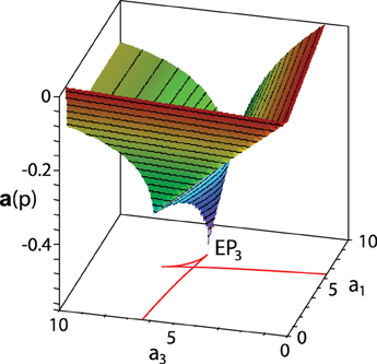
Figure 7. When a₂ is restricted to 10, the abscissa of (5) reaches its minimum at the triple negative real root $-\frac{\sqrt{3}}{3}$ when $a_1=4\sqrt{3}$ and $a_3=\frac{28}{9}\sqrt{3}$. The red curve is a cross-section of the discriminant surface (17) by the plane a₂ = 10.

In the region inside the “spike” formed by the discriminant surface all the roots are simple real and negative. Owing to this property, this region, belonging to the domain of asymptotic stability (see Figure 1), plays an important role in linear stability theory [29], as the next section demonstrates.

4. Heavily Damped Systems in Mechanics and Physics

Consider a linear mechanical system described by the equation [29]

where x(t) ∈ ℝ^m, t ≥ 0, and with the m × m matrices of viscous damping D and stiffness K both real, symmetric and positive definite. If the magnitude of the damping forces is big enough, one can expect that all the eigenvalues λ of the corresponding matrix polynomial L(λ) = λ² I + λ D + K will not only have negative real parts but be real and negative. The system (19) with semi-simple real and negative eigenvalues is called heavily damped [30]. The solutions of the heavily damped systems do not oscillate and monotonically decrease, which is favorable for applications in robotics and automatic control [31].

Note that in magnetohydrodynamics (MHD) there exists an inverse problem of excitation of instabilities by changing parameters of a heavily damped system. This is the famous MHD dynamo problem where by controlling the flow of an electrically conducting non-ideal fluid one has to excite and maintain magnetic field. At relatively slow and simple fluid motions the corresponding linearized equations define a heavily damped system with all its solutions decaying and non-oscillating, see [32–35]. Transition from non-oscillating to oscillating solutions in the dynamo problem is crucial for explanation of the geomagnetic field polarity reversals [36].

Assume that K is given and that we wish to choose the damping matrix D so as to ensure that all solutions to (19) decay to zero as rapidly as possible. This problem has been largely solved by Freitas and Lancaster [37]; see also [29].

Let α(D, K) denote the spectral abscissa of the matrix polynomial L(λ), that is the abscissa of its characteristic polynomial:⁹

The roots of the characteristic polynomial det(L(λ)) are the eigenvalues of the matrix polynomial L(λ) and also the eigenvalues of the 2m × 2m companion matrix

The optimal damping rate is determined by the solution of the optimization problem

Remarkably, Freitas and Lancaster [37] established that, for any K > 0,

with equality holding if and only if L(λ) has just one eigenvalue with algebraic multiplicity 2m.

In the case m = 2, this problem reduces to the one studied in the section 2. Since the constant term of the characteristic polynomial is det K, we introduce the quantities [15]

and following [37 Section 4], we reduce the characteristic polynomial of L(λ) to the form (5), except that the roots have been scaled by $\sqrt[4]{\det \text{K}}$. Conditions for asymptotic stability of the polynomial (5) are therefore given by (4).

Solving the system of equations a₁ = 4, a₂ = 6, a₃ = 4, where the coefficients a₁, a₂, and a₃ are defined by (20), yields an explicit expression for the damping matrix D that minimizes the spectral abscissa α(D, K) when m = 2 in terms of the coefficients k₁₁, k₂₂, k₁₂ and the eigenvalues ω²₁ and ω²₂ (ω_{1, 2} > 0) of the given matrix K. As shown by Freitas and Lancaster [37], but expressed here in different notation, given K > 0, we find that α(D, K) attains its global minimum with L(λ) having just one eigenvalue $\lambda =-\sqrt[4]{\det \text{K}}=-\sqrt{{\omega }_1{\omega }_2}$ with algebraic multiplicity 4 and geometric multiplicity 1, if D = D₊ or D = D₋, where [15]

Notice that D_± may be either positive definite or indefinite and that D₊ = D₋ if and only if K = κ I, where κ is a scalar [37].

Now we can give the following interpretation of the stability diagram of Figure 1. The dissipative system (19) is asymptotically stable inside the domain (4) with the coefficients a₁, a₂, and a₃ defined by (20). The boundary of the domain (4) has the Whitney umbrella singular point at a₁ = 0, a₃ = 0, and a₂ = 2. The domain corresponding to heavily damped systems of the form (19) is confined between three hypersurfaces of the discriminant surface (17) and has a form of a trihedral spike with the Swallowtail singularity at its cusp at a₁ = 4, a₂ = 6, and a₃ = 4; see Figure 3. The Whitney umbrella and the Swallowtail singular points are connected by the EP-set given by (13). At the Swallowtail singularity of the boundary of the domain of heavily damped systems, the abscissa of the characteristic polynomial of the damped potential system (19) attains its global minimum.

Therefore, by minimizing the spectral abscissa one finds points at the boundary of the domain of heavily damped systems. Furthermore, the sharpest singularity at this boundary corresponding to a quadruple real eigenvalue $\lambda =-\sqrt[4]{\det \text{K}}<0$ with the Jordan block of order four is the very point where all the modes of the system (19) with m = 2 are decaying to zero as rapidly as possible when t → + ∞.

5. Discussion

Typical singularities of the contour plots of the abscissa (or decrement diagrams) in the plane of two parameters were listed already by Arnold [19]. Let us have a closer look at the decrement diagram of the polynomial (5) shown in Figure 8. The additional constraint (a₂ = 10) removes the quadruple real root from the generic singularities; hence, the minimizer of the abscissa is the EP₃ point corresponding to the triple root $\lambda =-\frac{\sqrt{3}}{3}$ (see Figure 7, which shows the graph of the abscissa in three dimensions). The lower (curved) contours in Figure 8 correspond to the real parts of a complex-conjugate pair. The upper contours are straight lines and correspond to a simple negative real root. The contours cross either at the points of the discriminant set (17) corresponding to the double negative real roots (the lower part of the red cuspidal curve in Figure 8) or at the points where both complex conjugate roots and the real root have the same real part; see [19].

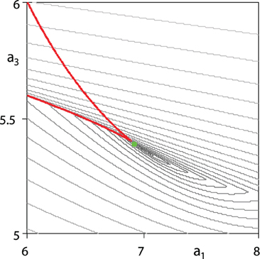
Figure 8. The gray curves show the contour plot (decrement diagram) of the abscissa a of the polynomial (5) when a₂ is restricted to 10. The green circle at the cusp of the red discriminant curve (17) marks the location of the EP₃ singularity, where the abscissa reaches its minimum in this case.

What are the relationships among the decrement diagram, stability boundary, discriminant set, and abscissa minimization? For a detailed answer it is simpler to consider a two-parameter cubic analog of the polynomial family (5)

and to look closely not only at the active roots, that is those whose real parts coincide with the abscissa a(p), but also at the remaining inactive roots, whose real part is algebraically smaller than a(p).

The polynomial (22) is Hurwitz if and only if

The discriminant curve of the polynomial (22)

bounds the domain of real roots in the (a₁, a₂) plane. It has a cusp singularity at a₁ = a₂ = 3; see Figure 9. In accordance with the Theorem of section 2 the polynomial abscissa a(p) has its global minimum at the singular EP₃ point of the discriminant curve corresponding to a triple root λ = −1.

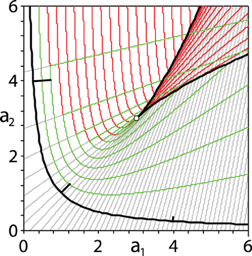
Figure 9. The green curves show the contour plot (decrement diagram) of the abscissa a of the cubic polynomial (22) with contour plots of the real parts of the inactive roots superimposed (red and gray curves). The open circle marks the location of the EP₃ singularity of the bifurcation diagram, where the abscissa reaches its minimum. The contours corresponding to simple real roots are straight lines that sweep out the cuspidal area confined between the boundaries of the bifurcation diagram. In the limit, these contours are tangent to the black cuspidal curve and may be viewed as rays forming a caustic [19, 42, 44]. The curved green contours correspond to real parts of a complex conjugate pair of eigenvalues. The black hyperbola marks the stability boundary with the stable region above it and to the right. Along the stability boundary, a few (negative) gradient vectors of the real part of the complex conjugate pair of active eigenvalues are marked at a₁ = 0.25, a₁ = 1, and a₁ = 4.

Denote

where the gradient of a root is given by the expression

For example, taking into account that at the points of the stability boundary (a₁a₂ = 1) the roots are

we find that the gradient of the real part of the complex-conjugate pair is

Figure 9 is plotted in the (a₁, a₂) parameter space. The black hyperbola shows the stability boundary, with the stable region (23) above and to the right. The small black strokes drawn at right angles to the hyperbola indicate some of the (negative) gradients (27).

The green curves and line segments in Figure 9 show the contours of the maximum of the real parts of the three roots of (22), i.e., they comprise a contour plot of the polynomial abscissa (the decrement diagram). More specifically, the green curves in the stable region correspond to a complex conjugate pair of active roots; in this region, as well as in the unstable region, the contours of the remaining inactive simple real root are shown by gray line segments. The green line segments appearing in the top part of the figure correspond to a simple real active root; in this region the contours of the real part of the complex conjugate pair of inactive roots are marked by the red curves.

Inside the cuspidal area whose boundary is exactly the discriminant curve given by (24), all three roots are real: the contours of the active root are marked by green segments, while the contours of the two inactive real roots are shown by red and gray line segments. In fact, the rays defined by the green, gray, and red line segments shown in the figure sweep out the cuspidal area. The boundary of the region of real roots can thus be viewed as a caustic or an evolute of the rays defining the contours of the negative real roots [19]. The open circle at the cusp is the EP₃ singularity, where the abscissa reaches its global minimum with all three roots equal to −1.

Despite the lack of smoothness and convexity of the abscissa and spectral abscissa functionals, numerical methods have been developed that are quite practical for finding local minimizers for arbitrary polynomial and matrix parameterizations—even when these minima correspond to multiple roots or multiple eigenvalues—provided the number of variables and the optimal multiplicities are not too large [38–41]. It may be interesting to interpret these or related methods in terms of rays and wave fronts propagating in the parameter space. Then, the powerful formalism of the theory of caustics and wave front singularities [42–44] could give a geometrical and even physical¹⁰ insight to the remarkable fact that globally minimizing the abscissa or spectral abscissa typically leads to multiple roots or multiple eigenvalues. Such an interpretation of polynomial root and matrix eigenvalue optimization algorithms as dynamical systems could be a line of research that is mutually fruitful for numerical analysis, stability theory, and mathematical physics.

Conflict of Interest Statement

The authors declare that the research was conducted in the absence of any commercial or financial relationships that could be construed as a potential conflict of interest.

Acknowledgments

Funding

The second author was supported in part by the U.S. National Science Foundation under grant DMS-1317205.

Footnotes

References

1. Ziegler H. Die Stabilitätskriterien der elastomechanik. Arch Appl Mech. (1952) 20:49–56. doi: 10.1007/BF00536796
2. Bottema O. The Routh-Hurwitz condition for the biquadratic equation. Indagationes Mathematicae (1956) 18:403–6.
3. Kirillov ON, Verhulst F. Paradoxes of dissipation-induced destabilization or who opened Whitney's umbrella? Z Angew Math Mech. (2010) 90:462–88. doi: 10.1002/zamm.200900315
4. Arnold VI. On matrices depending on parameters. Russ Math Surv. (1971) 26:29–43. doi: 10.1070/RM1971v026n02ABEH003827
6. Levantovskii LV. The boundary of a set of stable matrices. Russ Math Surv. (1980) 35:249–50. doi: 10.1070/RM1980v035n02ABEH001651
7. Levantovskii LV. On singularities of the boundary of a stability region. Mosc Univ Math Bull. (1980) 35:19–22.
8. Burke JV, Lewis AS, Overton ML. Variational analysis of the abscissa mapping for polynomials via the Gauss-Lucas theorem. J Global Optim. (2004) 28:259–68. doi: 10.1023/B:JOGO.0000026448.63457.51
9. Krechetnikov R, Marsden JE. Dissipation-induced instabilities in finite dimensions. Rev Mod Phys. (2007) 79:519–53. doi: 10.1103/RevModPhys.79.519
10. Vishik M, Lyusternik L. The solution of some perturbation problems for matrices and selfadjoint or non-selfadjoint differential equations I. Russ Math Surv. (1960) 15:1–74. (Uspekhi Math. Nauk. 15 (1960). 3–80).
11. Lidskiĭ, VB. On the theory of perturbations of nonselfadjoint operators. USSR Comput Math Math Phys. (1966) 6:73–85. (. Vyčisl. Mat. i Mat. Fiz. 6:52–60 (1966)).
12. Baumgärtel H. Analytic Perturbation Theory for Matrices and Operators (Operator Theory: Advances and Applications), Vol. 15. Basel: Birkhäuser Verlag (1985).
13. Moro J, Burke JV, Overton ML. On the Lidskii-Vishik-Lyusternik perturbation theory for eigenvalues of matrices with arbitrary Jordan structure. SIAM J Matrix Anal Appl. (1997) 18:793–817. doi: 10.1137/S0895479895294666
14. Maddocks JH, Overton ML. Stability theory for dissipatively perturbed Hamiltonian-systems. Commun Pure Appl Math. (1995) 48:583–610. doi: 10.1002/cpa.3160480602
15. Kirillov ON. Nonconservative Stability Problems of Modern Physics (De Gruyter Studies in Mathematical Physics), volume 14. Berlin, Boston: De Gruyter (2013). Available online at: http://www.degruyter.com/viewbooktoc/product/179816. doi: 10.1515/9783110270433
16. Trefethen LN, Embree M. Spectra and Pseudospectra: The Behavior of Nonnormal Matrices and Operators. Princeton, NJ: Princeton University Press (2005).
17. Henrion D, Peaucelle D, Arzelier D, Sebek M. Ellipsoidal approximation of the stability domain of a polynomial. IEEE Trans Autom Contr. (2003) 48:2255–9. doi: 10.1109/TAC.2003.820161
18. Henrion D, Lasserre J-B. Inner approximations for polynomial matrix inequalities and robust stability regions. IEEE Trans Autom Contr. (2012) 57:1456–67. doi: 10.1109/TAC.2011.2178717
19. Arnold VI. Lectures on bifurcations in versal families. Russ Math Surv. (1972) 27:54–123. doi: 10.1070/RM1972v027n05ABEH001385
20. Troger H, Zeman K. Zur korrekten modellbildung in der dynamik diskreter systeme. Ingenieur-Archiv (1981) 51:31–43. doi: 10.1007/BF00535953
21. Burke JV, Overton ML. Variational analysis of the abscissa mapping for polynomials. SIAM J Contr Optim. (2001) 39:1651–76. doi: 10.1137/S0363012900367655
22. Burke JV, Lewis AS, Overton ML. Optimizing matrix stability. Proc Am Math Soc. (2001) 129:1635–42.
23. Lewis AS. The mathematics of eigenvalue optimization. Math Program B (2003) 97:155–76. doi: 10.1007/s10107-003-0441-3
24. Burke JV, Lewis AS, Overton ML. Variational analysis of functions of the roots of polynomials. Math Program. (2005) 104:263–92. doi: 10.1007/s10107-005-0616-1
25. Berry MV. Physics of nonhermitian degeneracies. Czechoslovak J Phys. (2004) 54:1039–47. doi: 10.1023/B:CJOP.0000044002.05657.04
26. Heiss WD. The physics of exceptional points. J Phys A Math Theor. (2012) 45:444016. doi: 10.1088/1751-8113/45/44/444016
27. Blondel VD, Gürbüzbalaban M, Megretski A, Overton ML. Explicit solutions for root optimization of a polynomial family with one affine constraint. IEEE Trans. Autom. Control (2012) 57:3078–89. doi: 10.1109/TAC.2012.2202069
29. Veselic K. Damped Oscillations of Linear Systems (Lecture Notes in Mathematics), Vol. 2023, Heidelberg: Springer (2011). Available online at: http://www.springer.com/mathematics/applications/book/978-3-642-21334-2
30. Bulatovic RM. On the heavily damped response in viscously damped dynamic systems. J Appl Mech. (2004) 71:131–4. doi: 10.1115/1.1629108
31. Barkwell L, Lancaster P. Overdamped and gyroscopic vibrating systems. J Appl Mech. (1992) 59:176–81. doi: 10.1115/1.2899425
32. Arnold VI, Korkina EI. The growth of a magnetic field in a three-dimensional steady incompressible flow. Mosc Univ Math Bull. (1983) 38:50–4.
33. Kirillov ON, Günther U, Stefani F. Determining role of Krein signature for three-dimensional Arnold tongues of oscillatory dynamos. Phys Rev E (2009) 79:016205. doi: 10.1103/PhysRevE.79.016205
34. Giesecke A, Stefani F, Gerbeth G. Spectral properties of oscillatory and non-oscillatory α2-dynamo. Geophys Astrophys Fluid Dyn. (2012) 107:45–57. doi: 10.1080/03091929.2012.668543
35. Bouya I, Dormy E. Revisiting the ABC flow dynamo. Phys Fluids (2013) 25:037103. doi: 10.1063/1.4795546
36. Stefani F, Gerbeth G. Asymmetric polarity reversals, bimodal field distribution, and coherence resonance in a spherically symmetric mean-field dynamo model. Phys Rev Lett. (2005) 94:184506. doi: 10.1103/PhysRevLett.94.184506
37. Freitas P, Lancaster P. On the optimal value of the spectral abscissa for a system of linear oscillators. SIAM J Matrix Anal Appl. (1999) 21:195–208. doi: 10.1137/S0895479897331850
38. Burke JV, Henrion D, Lewis AS, Overton ML. Stabilization via nonsmooth, nonconvex optimization. IEEE Trans Automat Control (2006) 51:1760–9. doi: 10.1109/TAC.2006.884944
39. Burke JV, Lewis AS, Overton ML. A robust gradient sampling algorithm for nonsmooth, nonconvex optimization. SIAM J Optim. (2005) 15:751–79. doi: 10.1137/030601296
40. Lewis AS, Overton ML. Nonsmooth optimization via quasi-Newton methods. Math Progr. (2013) 141:135–63. doi: 10.1007/s10107-012-0514-2.
41. Overton ML. “Stability optimization for polynomials and matrices,” in Nonlinear Physical Systems: Spectral Analysis, Stability and Bifurcations, Chap. 16, eds ON Kirillov, and DE Pelinovsky. London: Wiley-ISTE, (2014). p. 351–75.
42. Arnold VI. Singularities of Caustics and Wave Fronts (Mathematics and Its Applications), Vol. 62. Dordrecht: Kluwer (1990).
43. Nye JF. Natural Focusing and Fine Structure of Light: Caustics and Wave Dislocations. Bristol: Institute of Physics Publishing (1999).
44. Ehlers J, Newman ET. The theory of caustics and wave front singularities with physical applications. J Math Phys. (2000) 41:3344–78. doi: 10.1063/1.533316
45. Yukawa T. Lax form of the quantum mechanical eigenvalue problem. Phys Lett A (1986) 116:227–30. doi: 10.1016/0375-9601(86)90138-6
46. Bloch A. Steepest descent, linear programming, and Hamiltonian flows. Contemp Math. (1990) 114:77–88. doi: 10.1090/conm/114
47. Brockett R. Dynamical systems that sort lists, diagonalize matrices, and solve linear programming problems. Lin Alg Appl. (1991) 146:79–91. doi: 10.1016/0024-3795(91)90021-N
48. Iserles A, Munthe-Kaas HZ, Nørsett SP, Zanna A. Lie-group methods. Acta Numerica (2000) 9:215–365.
49. Chu MT. Linear algebra algorithms as dynamical systems. Acta Numerica (2008) 17:1–86. doi: 10.1017/S0962492904
50. Moiseyev N. Non-Hermitian Quantum Mechanics. Cambridge, UK: Cambridge University Press (2011). Available online at: http://www.cambridge.org/us/academic/subjects/physics/quantum-physics-quantum-information-and-quantum-computation/non-hermitian-quantum-mechanics
51. Dietz B, Harney HL, Kirillov ON, Miski-Oglu M, Richter A, Schaefer F. Exceptional points in a microwave billiard with time-reversal invariance violation. Phys Rev Lett. (2011) 106:150403. doi: 10.1103/PhysRevLett.106.150403
Keywords: abscissa, optimization, overdamping, asymptotic stability, Whitney umbrella, Swallowtail, caustic, eigenvalue dynamics
Citation: Kirillov ON and Overton ML (2013) Robust stability at the Swallowtail singularity. Front. Physics 1:24. doi: 10.3389/fphy.2013.00024
Received: 08 October 2013; Paper pending published: 29 October 2013;
Accepted: 13 November 2013; Published online: 03 December 2013.
Edited by:
Pantelis Damianou, University of Cyprus, CyprusReviewed by:
Pantelis Damianou, University of Cyprus, CyprusPetre Birtea, West University of Timisoara, Romania
Copyright © 2013 Kirillov and Overton. This is an open-access article distributed under the terms of the Creative Commons Attribution License (CC BY). The use, distribution or reproduction in other forums is permitted, provided the original author(s) or licensor are credited and that the original publication in this journal is cited, in accordance with accepted academic practice. No use, distribution or reproduction is permitted which does not comply with these terms.
*Correspondence: Oleg N. Kirillov, Magneto-Hydrodynamics Division, Institute of Fluid Dynamics, Helmholtz-Zentrum Dresden-Rossendorf, PO Box 510119, D-01314 Dresden, Germany e-mail: o.kirillov@hzdr.de