Cognitive control in majority search: a computational modeling approach

Introduction

Our ability to rapidly process a vast amount of information and choose one out of several potential responses depends greatly on cognitive control – a mental function for prioritizing information processing (Posner and Snyder, 1975; Norman and Shallice, 1986; Posner and Rothbart, 1998). The role of cognitive control is most clearly manifested in performing various cognitive tasks such as the Stroop task and high-level planning. Although recent functional neuroimaging studies have revealed a set of brain regions that might be involved in cognitive control, the computational mechanisms underlying cognitive control remains debated (Posner and Dehaene, 1994; Desimone and Duncan, 1995; Botvinick et al., 2001; Wang et al., 2010).

The majority function task (MFT) is related to a common cognitive function in which one identifies the category to which the majority of items in a given group belong. For example, to answer simple questions like “Are there more boys than girls in the playground?” requires the computation of the majority function. While it would seem natural to assume that the computation depends greatly on cognitive control, the involvement of cognitive control in the MFT can be intriguing. On the one hand, algorithms for computing the majority function in computer science often imply little relevance of “control” in the process. In Boolean logic, for example, a majority function can be computed mechanically by a combinational circuit that output 1 if and only if more than half the inputs are 1’s (Cormen et al., 1994). For example, given three input bits x, y, and z, the majority can be computed based on the formula,

In artificial intelligence, one can implement the majority function using a perceptron with each input weight equal to 1 and the perceptron threshold equal to n/2, where n is the number of inputs (Russell and Norvig, 2003), again implying little involvement of cognitive control.

On the other hand, evidence has shown that cognitive control may play a much bigger role in human majority function computation than what these algorithms would suggest. In a recent study we evaluated possible algorithms underlying human performance using a computerized MFT (Fan et al., 2008). The participant was presented a set of horizontal arrows and had to decide the direction, left or right, in which the majority of the arrows pointed. Three algorithms were considered: exhaustive sequential search (sequentially scanning each and every one of the arrows and then making a final decision), self-terminating search (examining the arrows one-by-one and stopping as soon as a majority decision could be made), and grouping search (sampling and re-sampling the arrows with a sample size equal to the majority threshold until a congruent sample was found). The results showed that the grouping search algorithm fit the data best. Since the grouping search algorithm required that one determine the congruence for each sampled group (i.e., all arrows in the group point in the same direction), and in the case of incongruence, choose a different sample, the results indicated the systematic involvement of cognitive control.

The current study is to investigate the dynamics of cognitive control in the MFT from a computational modeling perspective. Using Leabra (O’Reilly and Munakata, 2000), a biologically realistic connectionist modeling framework, we have developed two neural network models. The two models are similar in that both involve the same set of neural modules representing task-relevant brain functions, share the same network connections, and are able to perform the task. However, by varying a single parameter, we show that they implement different algorithms that hold distinct implications for cognitive control. The modeling results show that they fit the human data differently, highlighting the critical role of cognitive control in the MFT.

Materials and Methods

The Majority Function Task

The MFT described in Fan et al. (2008) was a computerized task in which participants were presented with a set of horizontal arrows and had to decide the direction (left or right) that the majority of arrows pointed. In each trial, the arrow set was presented simultaneously, at locations randomly selected from eight possible ones arranged as an octagon centered on a fixation cross (see Figure 1). The set was shown for 2500 ms and participants were required to make a response by pressing one of the two keys as quickly and accurately as possible. Responses made within the 2500 ms window terminated the display of the arrow set, which was then followed by a variable fixation period of 2000–3000 ms, prompting participants to prepare for the next trial.

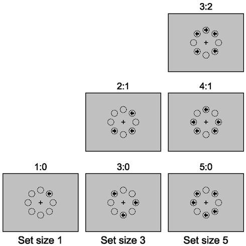
Figure 1. The majority function task (MFT). In this task, arrows with set size 1, 3, and 5 are randomly presented at eight possible locations arranged as an octagon centered on a fixation cross. The arrows point either left or right and are presented simultaneously. The participants’ task is to indicate the direction in which the majority of arrows point. For example, if three arrows are presented, and two point to the left and one to the right (see the “2:1” panel in the “set size 3” column), the correct response should be “left”. The eight circles are for illustration of the locations and are not displayed during the experiment. Different arrow composition conditions are shown for each set size.

The possible set sizes were 1, 3, and 5, so that the majority judgment was always unambiguous (the majority thresholds are 1, 2, and 3, respectively). Trials were blocked by set size. Different arrow composition conditions could be distinguished for blocks with set sizes of 1, 3, and 5. For set size 1, the majority was the same as the sole arrow itself (1:0). For set size 3, it was possible that two arrows pointed to the same direction (2:1) or all three arrows pointed to the same direction (3:0). Similarly, for set size 5, one could distinguish three composition conditions, 3:2, 4:1, and 5:0.

This experiment design allowed us to evaluate possible algorithms underlying human performance in the MFT (Fan et al., 2008). We started by analyzing the amount of information that the participant had to process in each condition before a decision could be made. We noticed that for any given stimulus display, different algorithms resulted in different amounts of information to be processed. Take the case of set size 3 as an example. A straightforward exhaustive search algorithm would require the participant to scan all three arrows before making the judgment. Assuming that each arrow scan processed 1 bit of information, this implied that the exhaustive search algorithm had to process 3 bits of information for set size 3, regardless of the arrow composition (2:1 or 3:0). This is different from the self-terminating search algorithm, according to which search stopped as soon as the majority could be decided upon (i.e., the number of same-direction arrows examined was equal to the respective majority threshold). Therefore, in the case of 3:0, only two arrow scans were necessary. In the cases of 2:1, the best scenario was two scans and the worst scenario was three scans. Because the probability of the best scenario was 1/3 in the experiment and the probability of the worst scenario was 2/3, the weighted average number of arrow scans in the case of 2:1 was 2 2/3. Finally, a grouping search algorithm was also possible. Based on this algorithm, a person could randomly select a sample of arrows (whose size was equal to the necessary majority size, two for set size 3 and three for set size 5) and check if they were congruent (i.e., pointing in the same direction) – a response could be made if the sample was congruent and a re-sampling was needed if it was not. Statistically the number of samples needed for a response (i.e., the first congruent sample, a success) follows a geometric distribution and the average is 1/p, where p is the probability of success. In the case of 2:1, for example, p is 1/3 and the average number of samples needed is 3. The average number of samples needed multiplied by the number of arrow in each sample leads to the average number of arrow scans in each condition. We then transformed these arrow scans to information measures in bits by taking the base 2 logarithm of the number of scans.

Assuming that the amount of information to be processed directly correlates with human performance (Hick, 1952; Hyman, 1953), we examined the mean human RT data as a function of the amount of information to be processed in different conditions (Fan et al., 2008). The exhaustive search algorithm was immediately ruled out because it did not fit the human data at all. For self-terminating search and grouping search, we noticed that while both algorithms could fit the human data, there was one major discrepancy with the self-terminating search – while the algorithm predicted that the 2:1 condition involved less information to-be-processed than the 5:0 condition (2 2/3 vs 3 bits, respectively), the human data revealed significantly longer RT in the 2:1 condition than in the 5:0 condition. Overall, the behavioral results supported the notion that humans tended to use the grouping search algorithm in the MFT.

Computational Models of the Majority Function Task

One possible explanation for the Fan et al. (2008) results is that the task requirements of the MFT encourage a grouping search algorithm. When a majority judgment is needed as soon as possible, one may take a betting strategy and choose to look at several items at the same time (e.g., subitizing), especially if the necessary sample size is not too large (as in the current MFT setup) and a successful sample can quickly lead to a response. Sequential-scanning based algorithms (either exhaustive or self-terminating), despite their simplicity, involve extra operations such as counting and remembering (e.g., “how many right arrows have been counted?”).

To further evaluate the plausibility of a grouping search algorithm in the MFT, it is important to examine how the mental operations subserving the grouping search might be instantiated in the brain. For example, one requirement for the grouping search strategy is a mechanism of grouping. A large body of literature in visual search has supported the notion of perceptual grouping (Treisman, 1982) and multi-object tracking (Pylyshyn, 2000, 2001). For example, it has been shown that human vision is capable of tracking multiple (usually less than 4) objects simultaneously (Pylyshyn, 2000, 2001). It is likely that similar mechanisms are used in the MFT to support grouping.

An even more important requirement for the grouping strategy is cognitive control, a mental function that is especially critical when the amount of information to be processed is overwhelming, or in the presence of salient distracters as in classical tasks such as the flanker task (Eriksen and Eriksen, 1974) and the Stroop color–word interference task (Stroop, 1935). Recent advances in human attention research have shown that cognitive control is an essential aspect of attention and is subserved by distinct networks in the brain, including areas in the prefrontal cortex and anterior cingulate cortex (ACC; Posner and Raichle, 1994; Miller, 2000; Fan et al., 2002; Posner, 2004; Roelofs et al., 2006). Since the grouping search strategy requires a judgment of group congruence, the involvement of cognitive control would be warranted. This is different from the sequential-scanning based algorithms, where the requirement for cognitive control is minimal. Therefore, analyses of the MFT performance directly lead to testable hypotheses of specific mental operations and neural correlates underlying the task performance.

Both issues can be addressed to a certain extent by developing and comparing computational models of human behavior in the MFT that implement different algorithms. Two such models were developed in this study, one for grouping search and the other for self-terminating search. By comparing the two models we show that the two models required different involvement of cognitive control and fitted human data differently. We argue that the models reveal a plausible way of cognitive control instantiation in the brain that underlies human performance in the MFT.

Results

General Model Description

The models were developed in the connectionist modeling framework of Leabra (for local, error-driven and associative, biologically realistic algorithm; O’Reilly, 1998; O’Reilly and Munakata, 2000). In contrast to other connectionist modeling frameworks, Leabra is a biologically realistic modeling framework with several unique features. For example, Leabra neurons use an activation function that models the known electrophysiology of real neurons closely while keeping the computation tractable. The connections among neurons in Leabra cannot freely change signs (i.e., changing from an excitatory link to an inhibitory link, and vice versa), which is allowed in earlier artificial neural network systems and has been shown to be biologically unrealistic. In addition, as a coherently integrated framework, Leabra allows different information transformation mechanisms and different learning algorithms (Hebbian learning, competitive learning, and error-driven learning) to simultaneously occur and interact. As a result, it is now possible to build deeper hierarchies of neural networks to simulate complex cognitive systems.

Brain networks

The networks in our models include not only the common regions for visual information processing such as V1 and V4 but also regions specifically selected based on recent cognitive neuroscience studies with similar information processing components as in the MFT. For example, an fMRI study on perceiving patterns in random sequences, similar to the serial-choice RT tasks used in early information theory studies, showed that violations of repeating patterns evoked activation in the prefrontal cortex, posterior rostral ACC, fronto-insular cortex, and basal ganglia (Huettel et al., 2002). RT and the amplitude of the hemodynamic response in these regions are associated with the length of the sequence before the violation. In another fMRI study, participants were presented with cue cards and asked to make a two-choice response to predict whether the next card would be higher or lower. Greater activation in the ACC and fronto-insular cortex was associated with higher uncertainty (Critchley et al., 2001). These regions have also been shown to be involved in conflict processing between possible responses (Nee et al., 2007; Wang et al., 2010). In addition, the lateral prefrontal cortex (LPFC) and posterior parietal cortex near/along the intraparietal sulcus (IPS) have been shown to be related to information processing evoked by the occurrence of a high information event (Strange et al., 2005; Yoshida and Ishii, 2006) and modulate the activity of early visual areas (Rossi et al., 2009). Finally, partially due to the functional similarity between IPS and frontal eye fields (FEF), we did not include the FEF in our models.

Model structure

These task-relevant brain regions were simulated in our models by layers (see Figure 2). In particular, each model contains seven layers with five having names roughly corresponding to those to-be-simulated brain regions. Each layer contains a certain number of neuron units, each of which does not literally correspond to a biological neuron per se but should be treated as a summary of a population of neurons for a specific function. The layers, described below, are connected in a biologically plausible way to form a network, similar to a previous model we built for simulation of attentional networks (Wang and Fan, 2007).

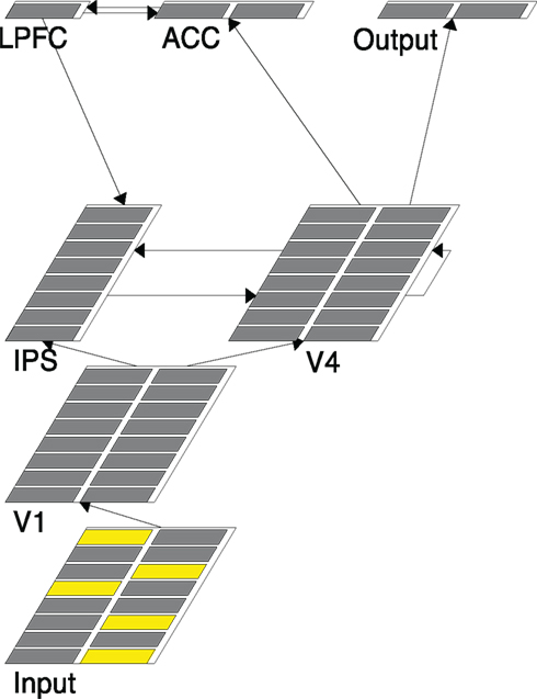
Figure 2. A snapshot of the model structure. Each layer simulates a brain region designated by the layer name. The five active units (yellow) in Input represent the five arrow stimuli presented in a trial.

(1) The Input layer has 16 units with an 8 × 2 configuration. Each row of units represents one location (so there are eight possible locations). The two units in the same row represent left pointing and right-pointing arrows, respectively. Figure 2, for example, shows that there are two left-pointing arrows and three right-pointing arrows that are presented.

(2) The V1 layer has the same configuration as that of the Input layer. It copies activations from the Input layer through a one-to-one projection (i.e., only corresponding units in the two layers are connected). Therefore it serves mainly as a placeholder for the information from the Input and does not literally correspond to the primary visual cortex.

(3) The V4 layer performs basic visual information processing and simulates the object selection and recognition networks in the brain. It has the same configuration as that of the V1 layer and connects from the V1 layer in a similar one-to-one projection. One critical difference is that the V4 layer performs a sampling/selective function on its V1 inputs. That is, it is possible that not all the units with active inputs from V1 actually fire in V4. In the five-arrow condition, for example, while there will be five units activated in V1 only a subset (1, 2, or 3) of those corresponding units in V4 may fire. This is implemented through a built-in mechanism in Leabra called k-winners-take-all (kWTA), which allows only a selected few, determined by the k setting, highest activated units in a layer to actually fire. Due to the noise in connection weights, the selecting processing can be stochastic. As will be shown later, this is a key mechanism used in our models to implement grouping (setting k of V4 to be 1, 2, or 3, depending on the condition) or a singleton selection (setting k of V4 to be 1).

(4) The V4 layer sends its output to the Output layer, which contains two units, representing the “left” and “right” response, respectively. Specifically, the “left” unit only connects to the eight units in the left columns of V4, and the “right” unit only connects to the eight units in the right columns of V4. The Output layer’s k is set to 1 to indicate that only one response is desired at a time. The firing threshold of the Output unit is set in such a way that normally it fires only when the number of active units with the same sidedness in V4 reaches the majority threshold. For example, in the five-arrow condition, at least three units in the left column of V4 have to fire in order for the left Output unit to fire. As soon as an Output unit fires the network halts, indicating that a majority decision has been made. The number of running cycles it takes for the network to get to this point is a measure of the model response time (O’Reilly and Munakata, 2000). We do not commit the Output layer to any specific region in the brain other than saying that it summarizes the information in the V4 layer and makes responses.

(5) The V4 layer also sends its output to the ACC layer, which then has a bidirectional connection with the LPFC layer. The purpose of these two layers is to monitor the activated units in V4 and detect incongruence (arrows pointing in different directions), if any, and therefore, simulate the function of cognitive control in the MFT. The ACC contains two units. The way it connects to the V4 layer is the same as the Output layer. However its k is set to 2 and no special firing threshold is set. The consequence of these settings is that an ACC unit fires whenever there is an activated unit in the corresponding column of V4. The ACC layer sends its output to the LPFC layer, which contains only one unit. The LPFC unit’s firing threshold is set in such a way that it typically fires only when both ACC units fire – suggesting that there are both left-pointed and right-pointed arrows in V4. Therefore, the LPFC layer detects incongruence by summarizing the information computed in the ACC layer.

(6) The IPS layer is specialized for spatial information processing and simulates the “where” pathway and the orienting attentional networks in the brain. It contains eight units organized in a column, representing the eight possible spatial locations where arrows can appear. The IPS layer sends its output to the V4 layer to enhance the processing of the corresponding V4 units. There are three sources from which the IPS layer receives input. First, it receives bottom-up input from the V1 layer. The connection from V1 to IPS is location-based, with two V1 units in each row connecting to the IPS unit in the corresponding row. Second, the IPS layer receives lateral input from (and sends output to) the V4 layer. The connection is again location-based, in a row-by-row fashion. Finally, the IPS layer receives top-down input from the LPFC layer, critical for the re-sampling function required in the grouping search model described later.

Model settings

The model uses most of Leabra’s default variable settings with a few task-specific changes summarized in Table 1. The settings can be classified into two categories. First, most of these settings (shown in regular font in Table 1) are tuned based on task-specific requirements – they are set that way so that the network is capable of performing the task in the first place. Consequentially they are set prior to the actual simulation and remain fixed in all experimental conditions. They are, therefore, not responsible for the main effects we intend to study (see Figure 4). Examples in this category include: (1) the accommodation time constant for integration in layers IPS and Output – a 0.02 setting makes accommodation in these layers a little faster so that a re-sampling can occur in a timely manner if necessary; (2) the activation threshold for units in the LPFC layer. This setting was to make sure that LPFC is fired when both ACC neurons are active; (3) all connection weights in the network were drawn from a uniform distribution with mean at 0.7 and variance at 0.1. The relative projection weight-scale between layers IPS and V4 was set to 0.5 to allow stronger bottom-up influence to avoid phantom activation in these layers (e.g., a right V4 neuron fires at a location where no arrow is presented in the input).

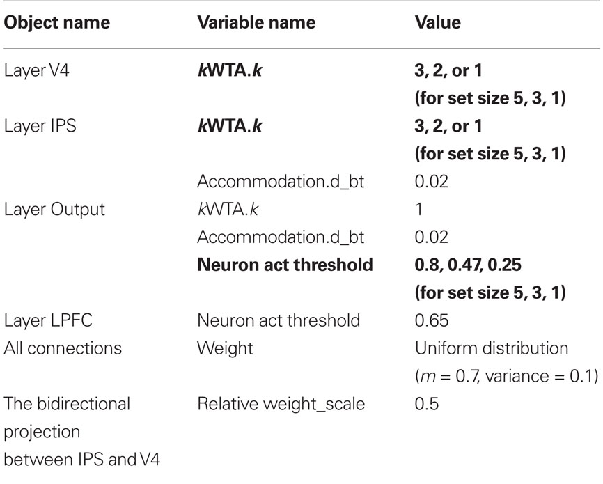
Table 1. Model settings (all variable settings remain fixed in all experimental conditions except those shown in bold).

Second, there are a few settings (shown in bold in Table 1) that are set based on each experimental condition and therefore are directly related to the main effects in Figure 4. They include the k setting in the V4 and IPS layers (3, 2, and 1 for conditions of set size 5, 3, and 1, respectively) and the activation threshold in the Output layer (0.8, 0.47, and 0.25 for conditions of set size 5, 3, and 1, respectively). Since each condition is presented in separate blocks (both in the behavioral study (Fan et al., 2008) and in our simulation), the k settings are set at the beginning of each block to designate subjects’ simple and necessary adjustment prior to that block (e.g., “Now each trial will contain five arrows, so I need to find three same-direction arrows as the majority”). To a certain extent the only “parameter” we tune to fit the data patterns in Figure 4 is the activation threshold in the Output layer, as it is systematically changed depending on the set size.

The Grouping Search Model

The essence of the grouping search model has to do with its ability to sample and re-sample the presented arrows with a given sample size. This is mainly realized via setting k in the V4 and IPS layers to be equal to the respective majority threshold in each condition. Therefore the model would select a group of k arrows (in V4) initially. If these k arrows happen to all point in the same direction (congruent), a response is made and the trial is over. Otherwise a new group of k arrows is selected and the searching continues.

We use Figure 3, showing the snapshots of the working model at two specific running cycles (left and right, respectively) in a given 3:2 trial, to describe how the grouping search model works. It is clear from the Input layer in Figure 3 that three left-pointing arrows and two right-pointing arrows are presented. Since this is in a five-arrow condition, the k of the V4 layer is set to be 3, the majority threshold. Figure 3A shows that at that particular moment (cycle 72) three arrows, one left-pointing and two right-pointing ones, are selected in V4. Of course this sample is not adequate to lead to a response – the right Output unit is preferred but not strong enough to reach the decision threshold. Therefore a re-sampling is necessary, which is implemented through the ACC–LPFC–IPS–V4 loop.

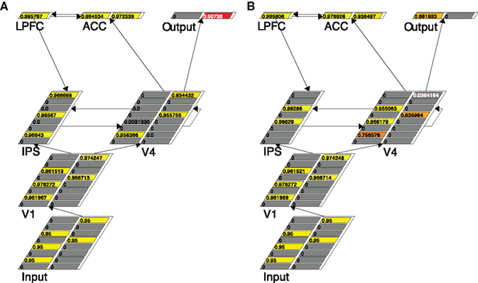
Figure 3. Traces of the grouping search model running in a trial with three left-pointing and two right-pointing arrows, at two different time points: cycle 72 (A) and cycle 106 (B). The number in each unit is its activation, also represented by color.

Specifically, in Figure 3A both units in ACC are activated, suggesting, correctly, that the selected sample contains both left-pointing and right-pointing arrows. This information is summarized by the firing of the LPFC unit, indicating incongruence has been detected. The IPS layer is notified of this incongruence through the LPFC–IPS connection, which leads to the higher activation in the IPS layer. As a result, the IPS units’ accommodation channels are turned on (by setting the units’ accommodation specification to true, a standard feature in Leabra). The effect of accommodation is that those units that have been active for a certain time are depressed so that units who lost the initial kWTA competition may have a chance to win and fire – a natural re-sampling. Note that since accommodation always punishes active units and rewards inactive units the re-sampling is not a random sampling in a strict sense. The re-sampling result in IPS is conveyed to the V4 layer through the bidirectional link between IPS and V4 so that re-sampling can also occur in V4 following the lead from the IPS layer. As shown in Figure 3B, at cycle 106 the two original quiet IPS units are activated (and the three originally activated IPS units accommodate), indicating two new arrow locations are selected. This location information is passed to the V4 layer, making the arrows in those locations relatively more active. The net result in this case is that more left-column units are activated, leading to the switch of preference in the Output layer. At cycle 114 the left Output unit finally reaches the response threshold and the model halts with a response.

Modeling results

For each trial, the model RT is measured by the number of cycles that the model takes to reach the majority decision. In the grouping search theoretically the number of cycles is determined by the number of samples (size k) scanned, which is determined by the configuration of stimulus set (e.g., 3:2 vs 5:0).

We ran the grouping search model 24 times to simulate 24 subjects, with each subject performing 12 trials of each task condition. The model was initialized (including both unit activations and connection weights) for each trial to induce necessary randomness and noise. Table 2 shows the modeling results. For ease of comparison we also list the empirical results reported in Fan et al. (2008). A visual inspection reveals that the modeling results, in both RTs (in cycles) and accuracies, show similar patterns as the empirical results. A mixed-effect linear model analysis shows that the mean RTs for the three set sizes (23.2 cycles, 53.8 cycles, and 88.6 cycles) were significantly different, F(1,140) = 46.24, p < 0.01. In set size 3, the RTs under the two conditions (2:1 and 3:0) were significantly different, F(1,44) = 313.87, p < 0.01. In set size 5, the RTs under the three conditions (3:2, 4:1, and 5:0) were significantly different, F(2,66) = 63.27, p < 0.01. More importantly, the RT in the 2:1 condition was significantly longer than the RT in the 5:0 condition, t(23) = 15.16, p < 0.01, consistent with the behavioral results in Fan et al. (2008).

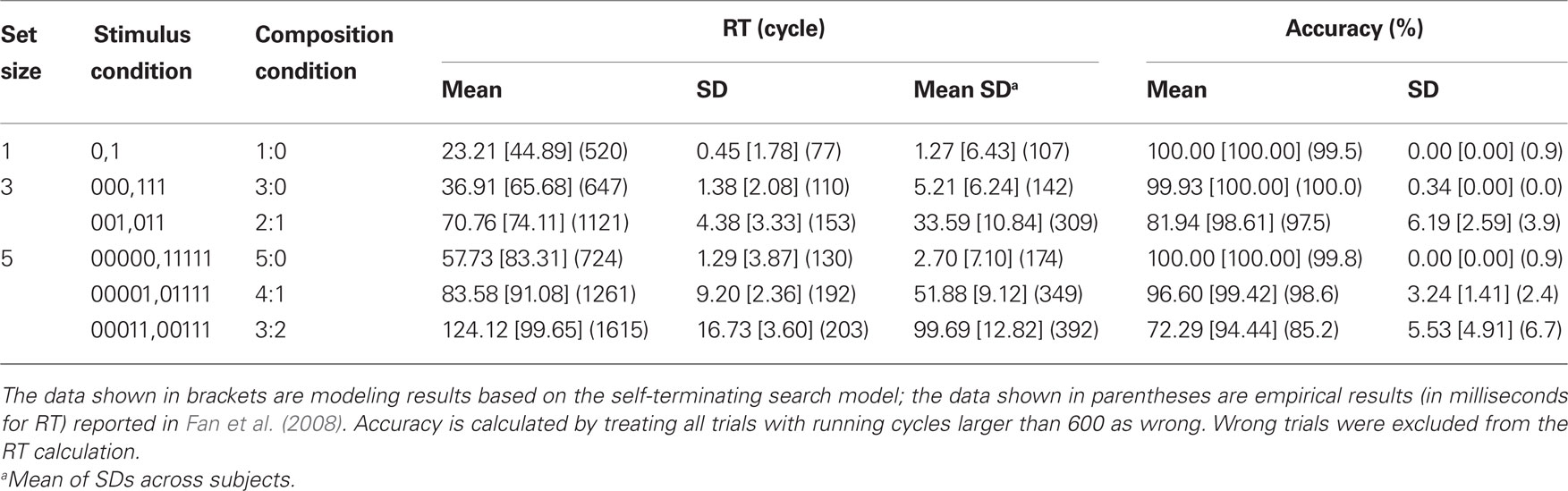
Table 2. The modeling results.

To further examine the model fit, we plot the mean modeling RTs (in cycles) as a function of task conditions, together with the empirical data from Fan et al. (2008), shown in Figure 4. It is clear that the model captures the main variance among task conditions. A linear regression of empirical RTs on modeling RTs reveals a R² of 0.95 [F(1,4) = 81.40, p < 0.01].

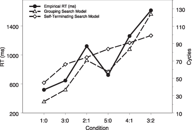
Figure 4. Computational modeling results (in cycles) as a function of task conditions, together with the empirical data (in milliseconds) reported in Fan et al. (2008).

The Self-Terminating Search Model

Structurally, the self-terminating search model is exactly same as the grouping search model. The main difference between the two models has to do with the k setting of layers V4 and IPS. Instead of fixing it to be the respective majority threshold in each condition (e.g., three in the five-arrow condition) as in the grouping search model, in the self-terminating model we set it to be 1 initially and gradually increase it (by 1 at a time) until a response can be made (i.e., when the number of active units with the same sidedness in V4 reaches the majority, three in the five-arrow condition, which then causes the corresponding Output unit to fire). This change leads to a self-terminating serial search in that the model essentially scans the presented arrows one-by-one and responds as soon as one Output unit reaches the firing threshold. In addition, by gradually increasing k rather than fixing it to be 1, the model basically selects a new arrow to scan at a time and keeps all those already scanned arrows actively represented in V4, thus emulating the counting component in a sequential-scanning based algorithm.

The mechanism for dynamically increasing the parameter k is implemented via a Leabra script, which in every running cycle monitors the number of currently active units in V4. If this number is less than the total number of arrows presented (i.e., not all arrows have been scanned) and the model has not yet responded, k is increased by 1. Note that the model responds as soon as one Output unit reaches the firing threshold – there is no requirement that a crucial number of arrows have to be scanned. In addition, the model leaves the ACC–LPFC–IPS habituation loop intact so conflict detection and re-sampling can still occur as in the grouping model. However, given the dominant effect of k increment these networks do not play a significant role in determining the model performance.

To demonstrate how the self-terminating model works, we again show the running trace of the model in a given 3:2 trial (see Figure 5). It shows that at cycle 40 only one right-pointing arrow (in V4) was detected (Figure 5A), at cycle 61 another left-pointing arrow were detected (Figure 5B), at cycle 76 an additional left-pointing arrow was detected (Figure 5C), and finally at cycle 90, another left arrow had been detected (Figure 5D). Given that at this moment three left-pointing arrows had been detected, the model then terminated with a left response, and the k setting of the V4 and IPS layers had now been increased to 4. The final RT measure was the number of cycles that it took for an Output node to fire.

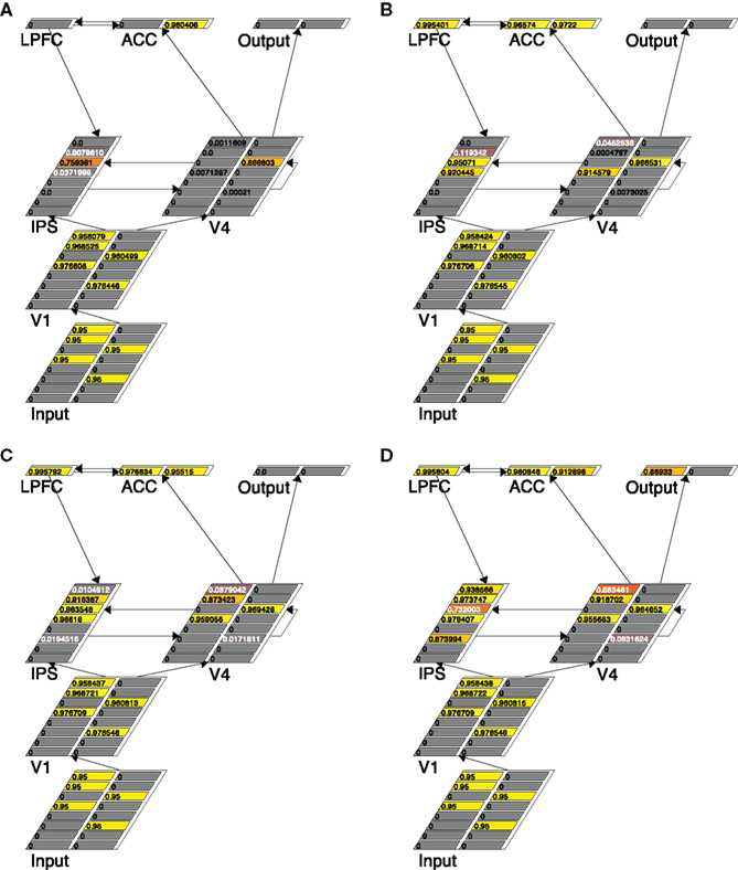
Figure 5. Traces of the self-terminating search model running in a trial with three left-pointing and two right-pointing arrows, at four different time points: cycle 40 (A), cycle 61 (B), cycle 76 (C), and cycle 90 (D). Note that the persistent activity in the IPS layer in the face of incongruity in the sample is mainly due to the dynamics generated by increasing k during the trial.

Modeling results

We again ran 24 simulated subjects with the model and the modeling results are shown in Table 2 and Figure 4, together with the grouping search model results and the data from human subjects. A visual inspection shows that a mismatch between the self-terminating search model results and the human data is evident. A mixed-effect linear model analysis shows that the mean RTs for the three set sizes (44.9 cycles, 69.9 cycles, and 91.4 cycles) were significantly different, F(1,140) = 276.53, p < 0.01. In set size 3, the RTs under the two conditions (2:1 and 3:0) were significantly different, F(1,44) = 36.28, p < 0.01. In set size 5, the RTs under the three conditions (3:2, 4:1, and 5:0) were significantly different, F(2,66) = 31.45, p < 0.01. Most importantly, the modeling RT in the 2:1 condition was significantly shorter than the modeling RT in the 5:0 condition, t(23) = −12.69, p < 0.01. This is inconsistent with the human behavioral results but consistent with what the self-terminating search algorithm predicts (Fan et al., 2008). A linear regression of empirical RTs on model RTs reveals a R² of 0.70 [F(1,4) = 9.30, p > 0.03], worse than the fit of the grouping search model.

Discussion

Cognitive control refers to processes that flexibly and adaptively allocate mental resources to permit selection of thoughts and actions directed by our intentions and goals under a certain context (Posner and Snyder, 1975; Miller, 2000; Badre, 2008; Kouneiher et al., 2009; Solomon et al., 2009), and has been implicated in a range of cognitive tasks involving attention, learning, and decision-making. Although the relationship between the activity of the frontoparietocingulate system and cognitive control has been consistently demonstrated in functional neuroimaging studies, the underlying computational mechanisms and dynamics of how these brain regions work together to implement the function of cognitive control remains unclear. The present study investigates the instantiation of cognition control by developing biologically realistic neural network models to perform a simple MFT, with the intention that the results can be extended to explain the computational underpinnings of cognitive control in other more complex tasks.

Search for the majority of a given item set is a common task and it is surprising that few studies have been conducted to understand how people perform the task. One reason may have to do with the fact that it can be easily done algorithmically, often via designed circuits or built-in functions. In statistics, the majority function is associated with mode, a statistic representing the value that occurs the most frequently in a data set, which is often readily shown by histograms. Fan et al. (2008) have developed a task to study how humans perform the majority function in a well-controlled environment. A careful analysis of the computational load required by different algorithms suggests that instead of using intuitive search strategies such as exhaustive search or self-terminating search, humans may adopt a grouping search algorithm, which involves sampling and re-sampling the item set with a majority-determining size.

It is important to note that the majority search, even in the context of MFT, is clearly relevant to ordinary visual search, on which a large body of research has been conducted (Treisman, 1982; Wolfe et al., 1989; Grossberg et al., 1994; Pylyshyn, 1994; Najemnik and Geisler, 2005). One might speculate that a possible pop-out mechanism exists for same-directional arrows in a stimulus set. However, given the close spatial proximity and perceptual similarity of the arrows, the perceptual basis of this pop-out is weak. In addition, the memory requirement (i.e., how many items in a given category have already been found) is greatly magnified in the MFT. As a result, in order to perform the task in a more efficient way, decisions of where to search next (which may not involve over eye movements) and when to make the response are critical, making a guided search a possibility (Niwa and Ditterich, 2008). However, to what degree such decisions depend on cognitive control has been unclear (Gray et al., 2006).

The grouping search algorithm makes distinctive claims regarding the involvement of cognitive control in the task than other more straightforward algorithms such as the self-terminating search. Based on the grouping search algorithm, for every selected group a judgment of group congruence has to be made, and in the case of incongruence a different group has to be selected and examined. Therefore, the algorithm implies the heavy and continuous involvement of cognitive control for conflict detection and re-sampling. This is different from those sequential-scanning based algorithms, where one can identify and count arrows one-by-one until a final decision can be made – no congruence judgment is explicitly necessary in these algorithms (Schall, 2001). On the other hand, the grouping search algorithm also implies that the task performance will be sensitive to the configuration of stimulus set. For those highly incongruent stimulus sets (e.g., three left arrows and two right arrows, compared to five left arrows), since the probability of selecting an incongruent sample is high, the likelihood of re-sampling is high, leading to longer reaction times.

A straightforward parallel search model, where all arrows in a presented stimulus set are simultaneously selected and processed (e.g., via setting k for the V4 and IPS layers to 5 in the five-arrow conditions), would presumably predict that all conditions of equal stimulus set size (e.g., 3:2, 4:1, and 5:0) have roughly same response time (i.e., the Output unit representing the majority will win out easily in all conditions). However, it is possible to augment this simple parallel search model with a mechanism to quantify the incongruence in a parallel fashion. For example, a mutual competition between two units in the Output layer (via setting its k to 1 in the current model) allows increased RTs in response to incongruent stimuli without engaging the whole V4–ACC–LPFC–IPS–V4 loop (see Gilbert and Shallice, 2002, for an example of incongruent competition in the context of Stroop effect). Neurally, such a mutual competition leads to activity normalization between two decision units, and neither unit would quickly reach a high decision threshold for a response (i.e., slow RT in this case) when they are comparably activated (e.g., driven by equally salient incongruent stimuli), leading to a pattern of RTs as a function of signal-to-noise ratio in evidence-based decision-making (e.g., Wong et al., 2007; Grossberg and Pilly, 2008). Note that in such a model the ACC–LPFC networks can still detect incongruence if any, but the effect of such detection could be too late to delay the response (i.e., an Output unit may have already fired). To a certain extent the grouping model can be regarded as an enhanced version of this augmented parallel search model in the sense that in the grouping model (1) a subset of stimuli can be simultaneously processed; and (2) the sensitivity to signal-to-noise ratio in different conditions is magnified by conflict detection through the V4–ACC–LPFC–IPS–V4 loop.

With advances in functional brain imaging, these claims lead to further hypotheses regarding possible brain activity and connectivity to support task performance. While it would be necessary to carry out functional brain imaging studies to examine the involvement of these brain areas, it is hard to reveal the dynamics of the brain in instantiating the computation. In the current study we show that we can study the dynamics of majority function computation in the brain by developing biologically realistic computational models of the task. In general a biologically plausible computational model that can perform the task in similar conditions as humans do and produce results that fit the human data provides not only an existence proof of the underlying algorithm but also a detailed process-based explanation for how the algorithm might be implemented in the brain (Marr, 1982; Anderson and Lebiere, 1998; O’Reilly and Munakata, 2000; O’Reilly, 2006; McClelland, 2009; Sun, 2009). Specifically, we developed two models of MFT performance, one simulating a grouping search algorithm and the other one simulating a self-terminating search algorithm. The two models share the same network structure and both are able to perform the task. Nevertheless, they involve the function of cognitive control differently.

The grouping search model demonstrates how modules simulating different brain functions work together to instantiate cognitive control for the majority function computation. Two critical components of the algorithm, sampling and re-sampling, are implemented through Leabra’s built-in kWTA mechanism and the joint work of the V4–ACC–LPFC–IPS loop. With k in V4 and IPS set to be the respective threshold in each condition, sampling is naturally implemented in V4. Because the network weights are randomly set, the initial sampling can be random as well. When a congruent sample is selected, a response can be quickly generated. When an incongruent sample is selected, the incongruence is detected and re-sampling occurs. More importantly, the model shows that cognitive control, important for the detection of incongruence in the selected sample and subserved by a set of neural modules, is recruited to modulate re-sampling. The longer RT in the 2:1 condition than that in the 5:0 condition, for example, is vividly explained by the frequent activations of the ACC and LPFC layers and the subsequent extra re-sampling processes in the 2:1 condition but the lack of those in the 5:0 condition. These results highlight the particular involvement of ACC and LPFC in implementing the function of cognitive control in the MFT and similar tasks.

It is interesting to note that the grouping search model can be revised to implement the self-terminating search, but the resulting model fails to fit the human data. The essential change concerns the k setting in V4 and IPS layers, which is gradually increased to simulate the sequential scanning and counting, a necessary component of the self-terminating search. The result that the self-terminating model fails to fit the human data to a certain extent provides further support for the claim that the grouping search model captures some essential constraints of cognitive control in the task. However, it is important to note that other models are certainly possible and many claims of the grouping search model are open to further experimental investigation. For example, it is possible to implement the self-terminating search more literally by fixing the k setting in V4 and IPS layers to be 1 (rather than gradually increasing it) and adding recurrent connections for both units in the model Output layer to achieve evidence accumulation over time as a way of counting. By doing so, although the model V4 explicitly samples one item at a time, a correct decision can still be made based on the sampling history maintained in the model Output layer.

Conclusion

We conclude by arguing that the different involvement of cognitive control differentiates the two models. In the grouping search model, the involvement of ACC and LPFC is essential since it is the function of these layers that detects conflict and eventually triggers and implements the re-sampling. On the contrary, in the self-terminating search model, the involvement of the ACC and LPFC functions is not required. Taken together, the models demonstrate how cognitive control might be instantiated in the brain to support the MFT.

Conflict of Interest Statement

The authors declare that the research was conducted in the absence of any commercial or financial relationships that could be construed as a potential conflict of interest.

Acknowledgments

This work was supported by an ONR cognitive science program grant (N00014-08-1-0042) and a Vivian Smith Foundation grant to Hongbin Wang, and a Young Investigator Award from the NARSAD and a NIH grant 1R21MH083164-01 to Jin Fan. We thank Kevin G. Guise and Frank Tamborello for assistance in various stages of the study.

References

Anderson, J. R., and Lebiere, C. (1998). The Atomic Components of Thought. Hillsdale, NJ: Lawrence Erlbaum Press.
Badre, D. (2008). Cognitive control, hierarchy, and the rostro-caudal organization of the frontal lobes. Trends Cogn. Sci. 12, 193–200.
Botvinick, M. M., Braver, T. S., Barch, D. M., Carter, C. S., and Cohen, J. D. (2001). Conflict monitoring and cognitive control. Psychol. Rev. 108, 624–652.
Cormen, T. H., Leiserson, C. E., and Rivest, R. L. (1994). Introduction to Algorithms. Cambridge, MA: MIT Press.
Critchley, H. D., Mathias, C. J., and Dolan, R. J. (2001). Neural activity in the human brain relating to uncertainty and arousal during anticipation. Neuron 29, 537–545.
Desimone, R., and Duncan, J. (1995). Neural mechanisms of selective visual attention. Annu. Rev. Neurosci. 18, 193–222.
Eriksen, B. A., and Eriksen, C. W. (1974). Effects of noise letters upon the identification of a target letter in a nonsearch task. Percept. Psychophys. 16, 143–149.
Fan, J., Guise, K. G., Liu, X., and Wang, H. (2008). Searching for the majority: algorithms of voluntary control. PLoS ONE 3, e3522. doi: 10.1371/journal.pone.0003522
Fan, J., McCandliss, B. D., Sommer, T., Raz, A., and Posner, M. I. (2002). Testing the efficiency and independence of attentional networks. J. Cogn. Neurosci. 14, 340–347.
Gray, W. D., Sims, C. R., Fu, W.-T., and Schoelles, M. J. (2006). The soft constraints hypothesis: a rational analysis approach to resource allocation for interactive behavior. Psychol. Rev. 113, 461–482.
Grossberg, S., Mingolla, E., and Ross, W. D. (1994). A neural theory of attentive visual search: interactions of boundary, surface, spatial, and object representations. Psychol. Rev. 101, 470–489.
Grossberg, S., and Pilly, P. K. (2008). Temporal dynamics of decision-making during motion perception in the visual cortex. Vision Res. 48, 1345–1373.
Huettel, S. A., Mack, P. B., and McCarthy, G. (2002). Perceiving patterns in random series: dynamic processing of sequence in prefrontal cortex. Nat. Neurosci. 5, 485–490.
Hyman, R. (1953). Stimulus information as a determinant of reaction time. J. Exp. Psychol. 45, 188–196.
Kouneiher, F., Charron, S., and Koechlin, E. (2009). Motivation and cognitive control in the human prefrontal cortex. Nat. Neurosci. 12, 939–945.
Najemnik, J., and Geisler, W. S. (2005). Optimal eye movement strategies in visual search. Nature 434, 387–391.
Nee, D. E., Wager, T. D., and Jonides, J. (2007). Interference resolution: insights from a meta-analysis of neuroimaging tasks. Cogn. Affect. Behav. Neurosci. 7, 1–17.
Niwa, M., and Ditterich, J. (2008). Perceptual decisions between multiple directions of visual motion. J. Neurosci. 28, 4435–4445.
Norman, D. A., and Shallice, T. (1986). “Attention to action: willed and automatic control of behavior,” in Consciousness and Self-Regulation, Vol. 4, Advances in Research and Theory, eds R. J. Davidson, G. E. Schwartz, and D. Shapiro (New York: Plenum Press), 1–8.
O’Reilly, R. C. (1998). Six principles for biologically based computational models of cortical cognition. Trends Cogn. Sci. 2, 455–462.
O’Reilly, R. C. (2006). Biologically based computational models of high-level cognition. Science 314, 91–94.
O’Reilly, R. C., and Munakata, Y. (2000). Computational Explorations in Cognitive Neuroscience. Cambridge, MA: MIT Press.
Posner, M. I., and Rothbart, M. K. (1998). Attention, self-regulation and consciousness. Philos. Trans. R. Soc. Lond., B, Biol. Sci. 353, 1915–1927.
Posner, M. I., and Snyder, C. R. R. (1975). “Attention and cognitive control,” in Information Processing and Cognition: The Loyola Symposium, ed. R. L. Solso (Hillsdale, NJ: Lawrence Erlbaum Associates), 55–85.
Pylyshyn, Z. W. (2001). Visual indexes, preconceptual objects, and situated vision. Cognition 80, 127–158.
Roelofs, A., van Turennout, M., and Coles, M. G. (2006). Anterior cingulate cortex activity can be independent of response conflict in Stroop-like tasks. Proc. Natl. Acad. Sci. U.S.A. 103, 13884–13889.
Rossi, A. F., Pessoa, L., Desimone, R., and Ungerleider, L. G. (2009). The prefrontal cortex and the executive control of attention. Exp. Brain Res. 192, 489–497.
Russell, S., and Norvig, P. (2003). Artificial Intelligence: A Modern Approach. Upper Saddle River, NJ: Prentice Hall.
Solomon, M., Ozonoff, S. J., Ursu, S., Ravizza, S., Cummings, N., Ly, S., and Carter, C. S. (2009). The neural substrates of cognitive control deficits in autism spectrum disorders. Neuropsychologia 47, 2515–2526.
Strange, B. A., Duggins, A., Penny, W., Dolan, R. J., and Friston, K. J. (2005). Information theory, novelty and hippocampal responses: unpredicted or unpredictable? Neural Netw. 18, 225–230.
Stroop, J. R. (1935). Studies of interference in serial verbal reactions. J. Exp. Psychol. 18, 643–662.
Sun, R. (2009). Theoretical status of computational cognitive modeling. Cogn. Syst. Res. 10, 124–140.
Treisman, A. (1982). Perceptual grouping and attention in visual search for features and for objects. J. Exp. Psychol. Hum. Percept. Perform. 8, 194–214.
Wang, H., and Fan, J. (2007). Human attentional networks: a connectionist model. J. Cogn. Neurosci. 19, 1678–1689.
Wang, L., Liu, X., Guise, K. G., Knight, R. T., Ghajar, J., and Fan, J. (2010). Effective connectivity of the fronto-parietal network during attentional control. J. Cogn. Neurosci. 22, 543–553.
Wolfe, J. M., Cave, K. R., and Franzel, S. L. (1989). Guided search: an alternative to the feature integration model for visual search. J. Exp. Psychol. Hum. Percept. Perform. 15, 419–433.
Wong, K. F., Huk, A. C., Shadlen, M. N., and Wang, X. J. (2007). Neural circuit dynamics underlying accumulation of time-varying evidence during perceptual decision making. Front. Comput. Neurosci. 1:6. doi: 10. 3389/neuro.10/006.2007
Keywords: cognitive control, uncertainty, majority function, algorithms, computational modeling, neural networks
Citation: Wang H, Liu X and Fan J (2011) Cognitive control in majority search: a computational modeling approach. Front. Hum. Neurosci. 5:16. doi: 10.3389/fnhum.2011.00016
Received: 02 September 2010;
Accepted: 25 January 2011;
Published online: 09 February 2011.
Edited by:
Francisco Barcelo, University of Illes Balears, SpainReviewed by:
Sara L. Gonzalez Andino, Hôpitaux Universitaires de Genèva, SwitzerlandTsung-Ren Huang, Boston University, USA
Copyright: © 2011 Wang, Liu and Fan. This is an open-access article subject to an exclusive license agreement between the authors and Frontiers Media SA, which permits unrestricted use, distribution, and reproduction in any medium, provided the original authors and source are credited.
*Correspondence: Hongbin Wang, School of Biomedical Informatics, University of Texas Health Science Center at Houston, 7000 Fannin Suite 600, Houston, TX 77030, USA. e-mail: hongbin.wang@uth.tmc.edu