Application of Airborne Infrared Remote Sensing to the Study of Ocean Submesoscale Eddies

Introduction

The recently discovered ocean realm of the submesoscale consists of density fronts and filaments, topographic wakes, and coherent vortices that have horizontal length scales of the order of 1 km, lifetimes of the order of 1 day, and values of Rossby number, Ro = ζ /f, of about one and larger, where ζ is the relative vertical vorticity and f is the local planetary vorticity (e.g., McWilliams, 2016). Submesoscale dynamics provides a transition between quasi two-dimensional flow and fully three-dimensional turbulence, and the resulting forward energy cascade provides a means to dissipate larger-scale energy. Submesoscale motions are further characterized by having relatively large vertical velocities that can alter ocean biogeochemistry by bringing nutrients into the sunlit zone and removing carbon from the upper ocean (e.g., Lévy et al., 2012).

Traditional oceanographic methods alone are inadequate for observing the submesoscale; novel methods, including remote sensing, must be employed to sample a large enough area with sufficiently high resolution. Thus, ocean submesoscale features have been investigated using synthetic aperture radar (SAR), deployed either on a satellite (e.g., DiGiacomo and Holt, 2001; Karimova and Gade, 2016) or aboard an aircraft (e.g., Marmorino et al., 2010). Visible-band satellite imagery has also been used, including the recent use of time-lagged (“stereo”) imagery (Delandmeter et al., 2017; Marmorino et al., 2017). While not yet widely used for studying the ocean submesoscale, infrared (IR) remote sensing can reveal dynamical processes that are largely invisible to other remote sensing techniques. Examples include the detection of near-surface turbulence associated with internal waves (Marmorino et al., 2008; Chickadel et al., 2018) and a “staircase” pattern indicative of frontal symmetric instability (Savelyev et al., 2018).

The Submesoscale Experiment (“SubEx”) was designed to collect high-resolution IR imagery, along with other remotely sensed and in-water data, in an investigation of fronts, filaments, and eddies in the Southern California Bight (Baschek et al., 2016; North et al., 2016). An objective was to capture the evolution of these features, including the circumstances of their creation and the mechanisms of their disintegration, as this would help fill a gap in the observational database of such dynamics. Here, we analyze airborne IR imagery of a submesoscale eddy collected during SubEx downstream of one of the several deep-water islands in the Bight. Our objectives are (1) to explore the use of thermal imagery to trace the surface flow, using a cross-correlation (“feature tracking”) technique; (2) to gain new insights into eddy kinematics and dynamics; and (3) to compare the results with in-water measurements.

Materials and Methods

Study Area

The measurements were made off the west end of Santa Catalina Island (33°30′N 118°31′W), a deep-water island located about 35 km south-southwest of the city of Los Angeles, CA. The northward-flowing Southern California Counter-Current as indicated in Figure 1 dominates mean flow. Numerical simulations reported by Dong and McWilliams (2007) show that positive vorticity can be shed from the western tip of the island, creating single coherent cyclonic eddies that subsequently advect downstream (Cyclonic in the northern hemisphere means counter-clockwise rotation). Such eddies are plausible candidates for the submesoscale “spiral eddies” seen in SAR imagery of the area, most of which suggest local cyclonic vorticity (DiGiacomo and Holt, 2001; Marmorino et al., 2010). Dong and McWilliams also found that the cyclonic eddies carry with them cold water upwelled during the eddy generation phase, with the result that the center of the eddy can be as much as 0.5°C cooler than the ambient surface water.

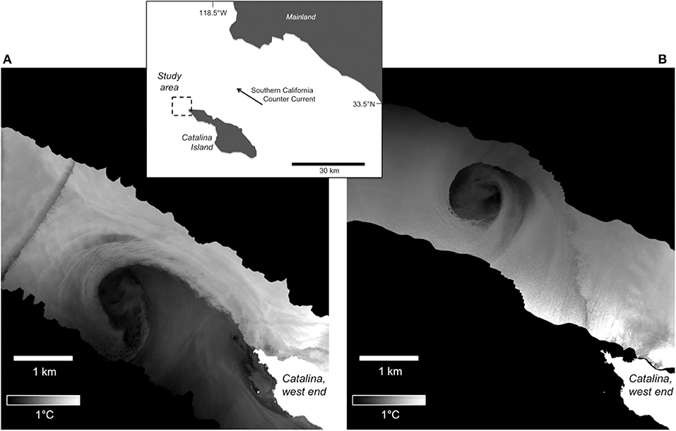
Figure 1. Infrared imagery showing two possible stages in the evolution of a cyclonic eddy downstream of Catalina Island (inset). (A) Early stage, eddy spinning-up directly downstream from the west end of the island. Isolated signature in the west is a boat wake. Data from 2 February 2013, 1824 UTC. (B) Later stage, showing cold eddy fully encapsulated by warmer water. Brighter areas along the southern edge of the image strip are sun-glint contamination. Data from 1 February 2013, 2026 UTC.

In airborne surveys collected on 30 January and 1–2 February, 2013, we observed three different cyclonic eddies initially located within 3.4 km of the west end of the island. Figure 1A shows one of these eddies (from 2 February) in the earliest stage of formation that we observed, spinning-up directly downstream from the island. Figure 1B shows a different eddy (1 February) in what we assume is a later stage of evolution. Somewhat contrary to the Dong and McWilliams study, the eddy in Figure 1B lies off the long axis of the island; but this may be related to effects not included in the simulations, such as tidal currents. Consistent with their prediction, the observed eddies do indeed have centers colder than the surrounding surface water.

Airborne Infrared Measurements

Infrared Camera and Deployment

Thermal imagery was collected using a mid-wave IR camera (model SC6000, Indigo Systems/FLIR, USA), having a frame size of 640 × 512 pixels, and an NETD (noise equivalent temperature difference) of < 0.02°C. Data were collected using a 25-mm lens and a framing rate of 30 Hz. The camera was deployed aboard a de Havilland DHC-6 Twin Otter aircraft, and oriented with the larger frame dimension perpendicular to the flight direction. Aircraft altitude and speed were typically ~3.7 km and ~50 m s⁻¹. Aircraft position and attitude were measured using a commercial GPS/INS (Global Positioning System/Inertial Navigation System; C-MIGITS III supplied by Systron Donner); these data are used to account for all aircraft motions, allowing geographical (“geo-”) referencing of the imagery to a relative accuracy of approximately 3 m.

The sampling strategy was that once an eddy was detected by scientists aboard the aircraft, the flight lines were re-oriented and shortened as needed to allow frequent repeat overpasses; these numbered from 10 to as many as 28 over two separate flights done on 2 February (North et al., 2016). Simultaneously, two research boats (see below) were vectored by the aircraft to the eddy's position. The subsequent, intensive crisscrossing of the eddy by the fast-moving boats tended to contaminate the IR imagery with long, persistent cold signatures induced by wake turbulence. Imagery from 1 February, however, is free of such effects (because the boats were delayed) and is therefore the focus of the present study. In addition to the data shown in Figure 1B (2026 UTC), 10 north-south overpasses of the eddy were made from 2034 to 2113 UTC (1234 to 1313 local time). These 10 overpasses are shown as an animation in the Supplementary Material.

Example of Consecutive Overpasses

It is helpful at this point to compare imagery from two consecutive overpasses of the eddy (Figure 2). The following key features will be examined in later sections:

(1) An abrupt boundary between the generally cooler interior of the eddy and the warmer ambient surface water. This will be referred to as the thermal perimeter of the eddy.

(2) An inflow in the southeast quadrant of the eddy of warm ambient surface water that moves cyclonically within the eddy, but which also has a component of motion toward the northern edge of the eddy (This can also be seen in the animation).

(3) Areas of small-scale cold patches, varying in size from 10 to 50 m, and ~0.2°C below ambient.

(4) A series of thermal bands spaced 30–70 m apart and lying just outside but nearly parallel to the eddy perimeter, most conspicuously in the southwest quadrant.

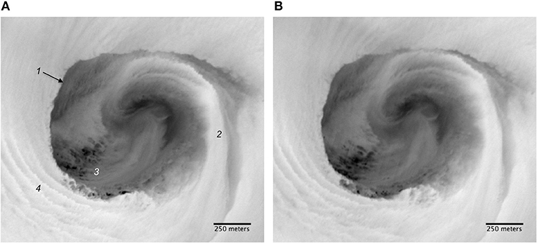
Figure 2. Infrared imagery from two consecutive overpasses on 1 February: (A) 2057 UTC; (B) 2101 UTC. Each panel shows a 1.75- by 1.5-km area of the ocean surface. Annotation in (A) indicates: (1) eddy perimeter; (2) warm inflow; (3) area of small-scale cold patches; (4) persistent azimuthal banding.

Each overpass thus shows thermal structure over a range of length scales. This structure, or image texture, is what allows the flow field to be deduced. A close examination of Figure 2, however, shows that much of the quickly evolving smaller-scale texture is incoherent between the two images, and this will result in spurious velocity retrievals in a feature-tracking calculation. But to obtain as complete, accurate, and detailed a portrayal of the flow field as possible, we want to exploit even the smallest-scale thermal structure. A procedure that allows this is discussed below (section Image Processing).

In-situ Measurements

Thermal structure within the water column was measured using a 100-m-long towed instrument array (TIA), which had nine temperature sensors spaced at depth increments of 0.4 to 10 m, sampled at intervals of 1 s, and having an accuracy of ±0.002°C. The TIA was towed at a speed of 4.3 ± 0.5 m s⁻¹, using a small maneuverable boat (a Zodiac), and provided data to a maximum depth of about 35 m. Profiles of water velocity from 2 to 12-m depth were measured using a 1,200-kHz acoustic Doppler current profiler (ADCP) mounted on a second research vessel, the R/V YellowFin. TIA transects began at 2157 UTC, about 44 min after the final IR overpass; ADCP transects began at 2249 UTC. Boat operations ended by 2400 UTC. An example of simultaneously acquired TIA and ADCP data are examined and compared with the IR data in section Comparison With in-situ Data.

Environmental Conditions

At the time of the measurements, meteorological conditions at Avalon, CA (33.34°N, 118.33°W), were as follows: wind speed, ~2 m s⁻¹; wind direction, north; air temperature, 20.0°C; dew point, 7.8°C; humidity, 45%; and a generally clear sky. Wave conditions measured at buoy 46222, located between Catalina and the mainland were: wave height, 0.71 m; period, 14.3 s; wave direction, 272°. Historical data from near the study location show that salinity stratification is usually negligible in the upper 80 m of the water column (Schneider et al., 2005); and conductivity-temperature profiles made just before and after towing the TIA showed salinity contributing to <10% of the density stratification.

Data Analysis

Image Processing

The IR images shown in this paper were created in a novel way, by processing a row of pixels from each data frame as would be done for a push-broom camera. In a push-broom camera, a single row of detectors arranged perpendicular to the flight direction and usually nadir-viewing (i.e., looking vertically downward) is used, along with appropriate data on platform elevation, attitude, etc., to synthesize a continuous view of the ocean surface as the aircraft flies forward. In the present study, the center row, or scanline, of each data frame was used to make an equivalently continuous geo-referenced image strip of the sea surface. To reduce the effect of sensor noise, 10 additional independently geo-referenced image strips were made using five rows to each side of the center row; then all 11 strips were then spatially averaged over 3-m square ground pixels to produce a single final image strip. The images shown in Figures 1, 2 were made in this way. The choice of 11 rows is somewhat arbitrary, but represents a balance between using enough rows to reduce noise, while not so many as would de-focus the image because of advection of features. Averaging over 11 rows corresponds to a temporal averaging over 0.8 s for each 3-m square pixel; so, for a surface current of 0.5 m s⁻¹, features are advected only 0.4 m.

Additional image strips were also made by separately using scanlines from the forward and rear edges of each frame. As such forward- and rear-constructed image strips are obtained from two different oblique viewing angles of a single camera's field of view, they form a stereo-like image pair; see Zhu et al. (2007) for a rigorous analysis. The significance for the present study is that, while these image strips cover a nearly identical area of sea surface, they are offset in time. The time difference Δt between forward and rear scans in this study lies mostly in the range of 32–34 s. This time difference is sufficient to detect horizontal motion on the sea surface (see below). To reduce noise, image strips based on 11 separate scanlines are again averaged over 3-m-square pixels to create the final forward and the rear image strips.

A comparison of forward and rear image strips (Figure 3) illustrates how small-scale thermal structure can be recognized in both views, thus providing a good tracer of any horizontal motion. As an example, a line drawn in the figure measures the distance between a randomly chosen cold patch and the eddy perimeter. The line is about 9 m shorter in the (later) rear image strip, suggesting the cold patch has moved radially outwards toward the perimeter by 9 m. As Δt = 32.4 s, that movement yields a relative surface velocity of 0.28 m s⁻¹. This value is greater than the nominal velocity detection threshold, which assumes translation of a feature across one pixel in time interval Δt; in the present case, 3 m /32.4 s = 0.09 m s⁻¹.

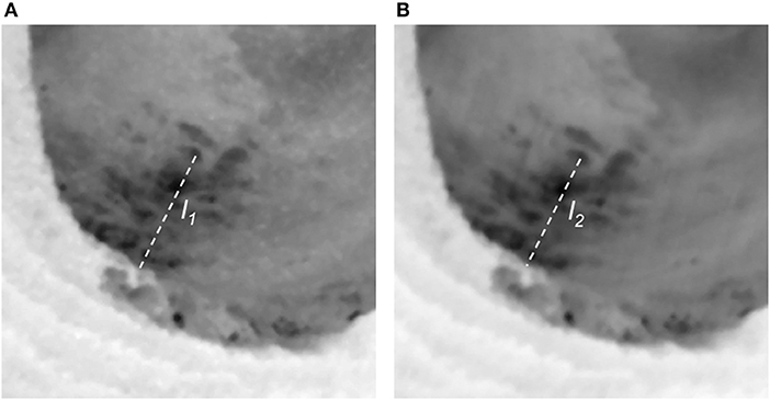
Figure 3. Enlarged view (600 m by 600 m) of the southwest part of the eddy, from the 2101 UTC overpass. (A) Image made using forward scanlines; (B) Image made using rear scanlines. The time difference between views is 32.4 s. Small-scale thermal structure can be seen to persist between views, and thus provides a good tracer of motion. Line (l₁) in (A), drawn between a randomly chosen cold patch and the eddy perimeter, is 201 m in length; a similarly drawn line (l₂) in (B) is shorter by about 9 m, thus indicating outward radial motion.

Estimation of the Velocity Field and Kinematic Quantities

Estimates of the surface velocity are derived from forward and rear image pairs using a normalized cross-correlation algorithm (Tseng et al., 2012) that is implemented as a “plugin” to the ImageJ processing and analysis package (Schneider et al., 2012). In this algorithm, an n × n pixel-sized interrogation window in the forward image is compared against a larger search area in the rear image. The difference in center positions of the interrogation window and its best match (highest correlation) within the search area is then selected as the displacement vector; the displacement vector divided by δt yields the velocity vector. A threshold of 0.6 is used in this study to identify vectors derived with low image correlations, resulting from an interrogation window presenting insufficient features (see below); such vectors are replaced by an interpolated value. Each successive interrogation window is displaced in the x and y directions by n/2 pixels (i.e., a 50% spatial overlap); the resulting velocity vectors thus have a physical spacing l equal to n/2 times the pixel width of 3 m. An “optimal” value of n is typically chosen as a compromise between spatial resolution and noise. For the example shown in the next section, n = 32; hence l = 48 m.

The resulting velocity field is used to compute the vertical component of vorticity ζ = ∂v/∂x – ∂u/∂y; the horizontal divergence δ = ∂u/∂x + ∂v/∂y; and the horizontal strain rate α = (N² + S²)^1/2, where N = ∂u/∂x - ∂v/∂y and S = ∂v/∂x + ∂u/∂y are the stretching and shearing components of the strain rate (e.g., Shcherbina et al., 2013). To help delineate vortex-like flow patterns from spurious signals, as well as from areas of linear shear, we make use of the swirling strength (Zhou et al., 1999). The swirling strength (units of s⁻¹) uses the imaginary part of the complex eigenvalue of the velocity-gradient tensor, and is calculated as λ_ci = ½ Im [(∂u/∂x – ∂v/∂y)² + 4 ∂u/∂y ∂v/∂x]^1/2. The differential kinematic properties of divergence, vorticity, and strain rate are important elements in describing the structure of relative motion, such as the deformation of a surface patch of tracer, and for relating the velocity field to dynamical processes (Molinari and Kirwan, 1975).

Results

IR-Derived Flow Field

Figure 4 shows results derived using the forward-rear image pair from the 2057 UTC overpass. These capture the key features of the flow field, and can be considered as representing a best case. The horizontal vector field (Figure 4A) shows a general cyclonic circulation over the entire scene. Areas having an outward radial component of flow occur along the southwest and northern parts of the eddy perimeter, consistent with the description in section Data Analysis. The cross-correlation coefficient (Figure 4B) is generally high (above our threshold value of 0.6) over most of the image scene, but areas having poor image texture have lower values (e.g., upper left and upper right) and indicate where interpolation was needed within the algorithm. The vorticity field (Figure 4C) indicates a central area, or core, of strong positive vorticity (> 1 × 10⁻³ s⁻¹). Areas of weaker vorticity occur nearer the perimeter of the eddy and in the warmer ambient water; weak negative values occur only in the corners of the scene. The vortex core is delineated even more cleanly in the swirling strength (Figure 4D). The core has an approximate diameter of about 570 m, while the thermal expression of the eddy has a diameter of about 1 km. Both the core and eddy extend slightly more in the east-west than north-south direction. Note that the warm inflow curves around the outer part of the vortex core. The divergence field (Figure 4E) shows near-zero values near the center of the eddy; areas of positive divergence near the outer edge of the vortex core; and areas of negative divergence (i.e., surface convergence) along much of the perimeter. The areas of convergence have signal levels as high as 1 × 10⁻³ s⁻¹. Estimates of strain rate (Figure 4F) are highest (>1.5 × 10⁻³ s⁻¹) between the vortex core and the eddy perimeter; averaged over the entire scene, the rms strain rate is 5.4 × 10⁻⁴ s⁻¹.

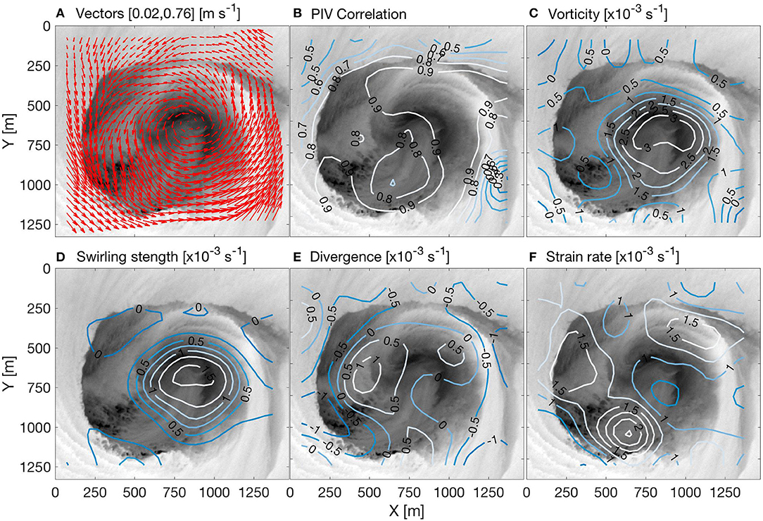
Figure 4. Velocity and kinematic properties derived from infrared data from 2057 UTC. (A) Vector field; (B) Cross-correlation peak; (C) Vorticity; (D) Swirling strength; (E) Divergence; (F) Strain rate.

Data from the other overpasses were analyzed similarly. All captured a core area of vorticity, though with some variability in shape and magnitude. Such variability we believe arises from various deficiencies and sources of noise in the data (section Challenges). To obtain overall mean values, we used the swirling strength to define the extent of the vortex in each overpass. Thus, averaging over all overpasses, the mean diameter is about 520 m (standard deviation of 40 m) and the mean vorticity is 2.2 × 10⁻³ s⁻¹ (standard deviation of 3 × 10⁻⁴ s⁻¹). This value of vorticity is equivalent to 27.4 times the local Coriolis parameter f = 0.803 × 10⁻⁴ s⁻¹. The corresponding solid-body rotational period is 1.6 h. The 39-min period shown in the animation thus corresponds to about 0.4 of a full rotation. Similarly, the more prominent areas of surface convergence were found to have overall mean of 7.2 × 10⁻⁴ s⁻¹ (standard deviation of 2.4 × 10⁻⁴ s⁻¹).

Comparison With in-situ Data

Figure 5A shows the nearly simultaneous sampling tracks of the Zodiac (TIA) and R/V YellowFin (ADCP) made from ~ 2300 to 2315 UTC. The final IR image (from 2 h earlier) is shown to provide perspective, but it is the large white circle (1-km in diameter) that indicates the eddy's likely location at the time of the boat measurements. The TIA-measured temperature section (Figure 5B) shows the hydrography of the upper 30 m. The key feature is an uplift of deeper layers of cold water. In particular, the peak of the 12.5°C isotherm was used to estimate a center position for the eddy (the red dot in Figure 5A), and this is used as the origin of the radial axis in Figure 5B. Near-surface water within the eddy is (as expected) cooler than the ambient water, and it is stratified. The dashed curve in Figure 5B will be explained in section Dynamical Link to the Thermocline.

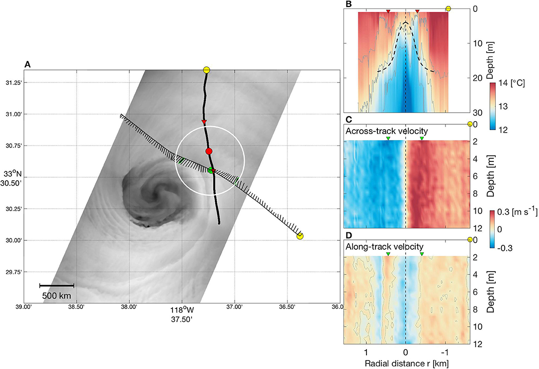
Figure 5. Representative in-situ data. (A) Nearly simultaneous sampling tracks of the R/V YellowFin (curve with 2-m depth velocity vectors; 2259–2315 UTC) and the Zodiac (bold curve; 2302–2309 UTC). The image shows the final IR overpass, which was made about 2 h earlier (2113 UTC). A 1-km-diameter circle indicates the eddy's approximate location at the time of the boat measurements. Yellow dots show the beginning location of the boat transects; the red dot is the eddy center estimated from the temperature data, and the green dot from the across-track velocity. (B) Vertical temperature section plotted against distance from the eddy center. Red triangles indicate maxima in surface temperature gradient. Superimposed dashed curve shows modeled depth of 13°C isotherm, using Equation (5) in the text. (C,D) Vertical sections of across-track and along-track velocity components, plotted against distance from the eddy center. For reference, green triangles indicate maxima in across-track speed.

Vertical sections of the across- and along-track velocity components measured by the ADCP are plotted in Figures 5C,D. In this case the eddy center (r = 0) is estimated from the across-track velocity. Note that the ADCP-based eddy center (the green dot in Figure 5A) lies about 250 m south of the TIA-based center. Neither the across- nor along-track component shows significant vertical shear. Velocity magnitude vs. radial distance is plotted in Figure 6A, where results from the southeastern and northwestern halves of the boat track are shown separately as the red and blue curves. The magnitude increases rapidly with distance from the center position, the bulk of the increase occurring within the first 250 m. This is similar to an IR-derived radial profile of velocity magnitude (the dashed curve in Figure 6A), which was computed by azimuthally averaging the vector field in Figure 4A.

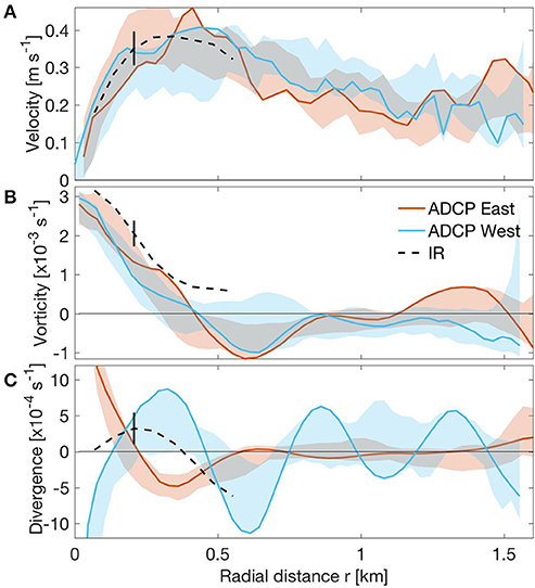
Figure 6. ADCP vs. IR estimates of velocity magnitude (A), vorticity (B) and divergence (C) plotted against radial distance. ADCP-derived values of vorticity and divergence are computed using Equations (1, 2) in the text. Red curves use data from the half of the boat track lying south-east of the vortex center; blue, the half north-west of center (c.f., Figure 5A); corresponding shading shows variability with depth. Dashed curves show IR-derived radial profiles after azimuthally averaging the results in Figure 4; vertical error bars at r = 200 m indicate a range of two standard deviations.

Vorticity and divergence are estimated from the ADCP data using cylindrical coordinates (r, θ). The radial velocity component V_r is thus derived from the along-track velocity component, and the azimuthal component V_θ from the across-track component. If it is assumed there is no azimuthal variation in the flow, then the expression for vorticity can be written as

Figure 6B shows a plot of ζ as a function of r, again shown separately for the two halves of the boat track. The ADCP-derived signal decreases approximately linearly from a maximum of about 3 × 10⁻³ s⁻¹ at the origin to zero at r = 0.43 km, beyond which it is negative out to about 0.8 km. The IR-derived vorticity (dashed curve) shows somewhat larger values but parallels the ADCP result until leveling off at about 0.5 × 10⁻³ s⁻¹, which can probably be taken as noise level (c.f., Figure 4C).

The corresponding expression for divergence is

It is plotted as a function of r in Figure 6C. It is a difficult result to interpret. The problem arises from the radial (or along-track) velocity component not being zero at the “center” of eddy; it is in fact negative (Figure 5D), as would the case if the true center lay somewhat north of the ADCP estimate. This results in the two halves of the boat track curves having opposing signs in the region r < 0.5 km; these signals are not relevant to the present discussion. What is relevant, we believe, is the large negative signal in the blue curve of about −1.1 × 10⁻³ s⁻¹ at r = 0.6 km, as this would correspond to convergence along the edge of the eddy; this result is consistent with the areas of large convergence in Figure 4E.

Dynamical Link to the Thermocline

A general question is whether remotely sensed data can be used to deduce the sub-surface structure of the water column. In particular can the IR-derived properties of the vortex be used to estimate an expected uplift of the lower water layer? To attempt this, we use a Rankine vortex as a highly idealized representation of our eddy. The Rankine vortex has an azimuthal rigid-body flow in a core of radius R, and irrotational azimuthal flow (i.e., zero vorticity) outside that region. The velocity profile can be expressed as

where V = V_θ (R) is the maximum velocity. V is related to the vorticity inside the core, ζ_core, by

An expression for thermocline displacement can then be derived under the following additional assumptions:

(1) The ocean consists of a homogeneous upper layer of thickness h(r), and a lower layer that is denser and dynamically passive (i.e., motionless).

(2) The upper-layer velocity is specified by Equations (3a,b).

(3) The dynamical balance is cyclostrophic, with a balance of radial pressure gradient and centrifugal force), so we can write

where g′ = g Δρ/ρ is the reduced gravity and Δρ/ρ is the relative density difference between layers.

Integration of Equation (4) then yields

where continuity of h has been imposed at r = R, and h(∞) is the upper-layer thickness at some appropriately large value of r outside the eddy.

To evaluate Equations (5a,b), model parameters are chosen from the IR results as R = 260 m and ζ_core = 0.0022 s⁻¹. For consistency within the model, we use Equation (3c) to derive V = 0.30 m s⁻¹. We use the 13°C isotherm in Figure 5B as the interface between upper and lower layers. The upper-layer temperature is captured best at large values of r, and is estimated by the transect's maximum temperature (14.2°C); the lower-layer temperature by the lowest values near r = 0, and is estimated by the transect's minimum temperature (11.79°C). Assuming salinity is constant (section Environmental Conditions), the corresponding density difference is Δρ = 0.616 kg m⁻³; thus g′ = 0.0059 m s⁻². The depth of the 13°C isotherm at a radius of r = 750 m is used as h(∞). The resulting h(r) curve is shown superimposed on the temperature section (Figure 5B; dashed curve). While we cannot expect a faithful reproduction of the overall thermal structure, the model does seem able to capture approximately the steep rise of the 13°C isotherm, as well as an uplift of about 14 m. Thus the essential doming of the isotherms is in reasonable correspondence with the data over the inner part of the eddy, and this helps confirm that the vortex and uplifted thermocline are dynamically linked.

Discussion

Kinematic Properties

A key result is the high value of vorticity, ζ = 27f, found within the core of the eddy. While comparable values have been measured in association with strong flow through an inlet or past small shallow-water islands (Delandmeter et al., 2017; Marmorino et al., 2017), this is a very large value for the open sea. Ohlmann et al. (2017) made surface Lagrangian measurements in several fronts and eddies during SubEx. Their analysis of the evolution of four-drifter clusters deployed in eddies (including the eddy shown in Figure 1A) yielded an overall mean vorticity value of 5.4f. This is also a large value, though possibly an underestimate as, given that the drifter sampling distances ranged from 0.3 to 4 km, it is unlikely an entire drifter cluster ever fully lay within an eddy's core. Curiously, Ohlmann et al. also found that drifters deployed in eddies showed a mean divergence value of +2.3f, which as they point out is a puzzling result. Possibly here, too, the drifter sampling distance plays a role: e.g., if some drifters (even one) were to become trapped in a core while others were free to move away, that could result in an apparent, but artificial, flow divergence. As for strain rate, its measurement for submesoscale flow fields is rare. Berta et al. (2016) report values of about 2f in the northern Gulf of Mexico, using surface drifters with a sampling distance of 100 m; our estimate of about 7f is larger, but of the same order of magnitude.

Eddy-Scale Circulation Pattern

The large value of vorticity indicates the importance of the centrifugal force in the dynamical balance of the eddy. This was explored with a simple model. It showed an upward doming of the thermocline of the order of 14 m at the center of the eddy. In the ocean, this effect could be expected to enhance the local growth of phytoplankton. Also, the large vorticity and small radius suggest the core should be highly (inertially) stable, which means the water in the core should not readily interact with water outside it. One can speculate, therefore, that material can remain trapped within the central part of the eddy and be transported along with it.

In addition to cyclonic rotational motion, the image analysis shows outward radial flow. As a consequence of the radial flow, there is convergence along the eddy perimeter. This is supported by the in-situ measurements. The convergence leads to downward motion and enhanced vertical exchange, similar to what occurs along a surface front. We suspect that without such radial flow, the thermal perimeter of the eddy could not be maintained in a steady state. Other aspects of eddy morphology, such as the comma or spiral shape visible in Figure 5, are beyond the scope of the present study to investigate.

Smaller-Scale Dynamics

Because the near surface is stably stratified by temperature, vertical stirring and turbulent mixing will produce a relatively cold surface imprint. It is probable that the cold patches in our imagery are such imprints. These features persist on the surface for at least 30 s (Figure 3), but not for as long as 4–5 min, which is the time interval between successive overpasses (Figure 2). It is interesting that distinct cold patches recur in some areas of the eddy but are not apparent in others areas, at least over the duration of the IR measurements. The imagery thus provides some information about where in the eddy turbulence is most intense or at least shallow enough to alter the sea surface temperature. The occurrence of similar cold features within eddies from other days, such as 2 February (Figure 7; highlighted area), suggests near-surface turbulence is an integral part of the eddy dynamics. We can also note that such turbulence can have an underlying, spatially periodic structure in some of the imagery. This is clear in the 2-February eddy (Figure 7), which shows a banded structure with spacing in the range of 30 to 50 m; but less clear in the 1-February eddy, though Figure 2A shows some evidence for it.

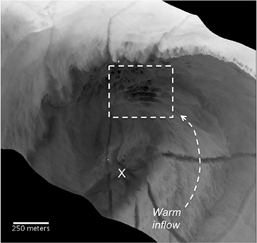
Figure 7. Infrared imagery of an eddy sampled on 2 February, and which exhibits features similar to those in Figures 2, 3. An “X” indicates the approximate rotational center of the eddy; arrow indicates ingestion of warm water from the south; box highlights an area of regularly spaced bands of cold patches. Multiple, long dark signatures are cold wakes from two research boats, which themselves appear as bright objects in the image. Data were acquired 1.8 h after that shown in Figure 1A.

It is interesting that the azimuthally oriented banding associated with the 1-February eddy (feature 4 in Figure 4) has a not dissimilar spacing of 50–70 m. That banding persists over the entire period of aircraft sampling (47 min) with relatively little change (Figures 1, 2, 7; see also animation). This suggests the banding was either created before our observations began and did not evolve subsequently, or was created continuously during the observation period. Our view tends toward the latter; but how the banding arises, and why it has the spacing and spatial extent that it does, are questions for future work. At this point, a reasonable conjecture is that such features arise from vertical shear instability (e.g., Zhou et al., 2017).

Note that the evidence for vertical mixing and flow instability, as well as aspects of the flow pattern discussed earlier (e.g., the outward radial flow), would be difficult if not impossible to obtain using a passive technique other than infrared remote sensing.

Challenges

A number of challenges present themselves during the collection, processing, and analysis of the imagery. First, unlike laboratory experiments in which the flow can be seeded uniformly with discrete particles, we rely on naturally occurring thermal features to produce image texture. It is usually the case, however, that this texture is not uniformly good throughout an entire image scene. In our case, there are areas both within the eddy and in the ambient water where image texture is poor or completely lacking; furthermore, because the morphology of the eddy changes over time, the areas having good and poor texture vary. The result is that not every pair of image scenes yields a satisfactory velocity field. Additionally, noise arises in the imagery from environment factors and effects related to the sensor and data processing. These include: contamination from sun glint in one or another of the pair of images, depending on which had the more southward look; incomplete correction for variable-length atmospheric-path radiance; atmospheric thermal inhomogeneity (Clark, 1967); and an along-track “striping” texture that is induced by calibration offsets across the detector elements. Use of a long-wave IR camera in future work would reduce sun glint, and remedies for other issues are under investigation; but that the other issues can be ameliorated to a significant extent is speculation at this point. Also important is that aerial surveys be conducted with many repeat lines in a reproducible way, covering the same area of ocean feature on each overpass, while maintaining the same aircraft altitude and sensor orientation. Coordination with research boats is another issue that requires care, e.g., wakes can quickly contaminate the thermal signals of interest.

Conclusions

The results show that high-resolution infrared remote sensing can provide useful and unique information about the ocean submesoscale. The essence of a submesoscale eddy is revealed through analysis of airborne infrared imagery, despite some flaws in the specific dataset examined here. After processing the imagery in a way that preserves the smallest-scale features, the structure within the thermal fields is generally adequate as a tracer of surface fluid motions. A key result is the very large vorticity in the core of the eddy, corresponding to a Rossby number of about 27. This indicates the importance of the centrifugal force in the dynamical balance of the eddy, and the correspondingly large central uplift of the thermocline as measured by the in-water transect. The analysis is able to indicate where sinking motion is likely strongest and to provide a glimpse of where kinetic energy cascades to turbulence. Our study has also raised a number of questions and speculations, such as whether material is trapped within the core, and what the origin is of various banded patterns. These can be addressed in a program of future research.

Author Contributions

BB, GS, and GM contributed to experiment planning and data collection. GS had primary responsibility for deployment of the airborne infrared instrumentation and post-processing of the imagery, including the geo-referencing. BB designed the towed instrumentation and data collection system, and was chief scientist for the submesoscale experiment. All authors contributed to analysis of the data, interpretation of results, and the writing of the manuscript.

Conflict of Interest Statement

The authors declare that the research was conducted in the absence of any commercial or financial relationships that could be construed as a potential conflict of interest.

The handling Editor declared a shared affiliation, though no other collaboration, with two of the authors, GM and GS.

Acknowledgments

GM and GS were supported by the Office of Naval Research through Naval Research Laboratory project 72-1C02-07; the present work is contribution number NRL/JA/7230–17-0327. RN and BB were supported by the Helmholtz Program Polar Regions and Coasts in a Changing Earth System (PACES II) and NASA-Grant NNX10AE94G.

Supplementary Material

The Supplementary Material for this article can be found online at: https://www.frontiersin.org/articles/10.3389/fmech.2018.00010/full#supplementary-material

Supplementary Video 1. This shows an animation of 10 overpasses made on 1 February 2013, from 2034 to 2113 UTC. The average time between images is 4.3 min, and the area shown is 1,800 m by 1,350 m. The images have been aligned to have an approximately common dynamical center, i.e., center of rotation of the eddy.

References

Baschek, B., Smith, G. B., Miller, D., Angel Benavides, I. M., North, R. P., and Marmorino, G. O. (2016). “High-resolution observations of submesoscale eddies in the coastal ocean,” in Abstract (OS16-EC14A-0964) Presented at 2016 Ocean Sciences Meeting (New Orleans, LA).
Berta, M., Griffa, A., Özgökmen, T. M., and Poje, A. C. (2016). Submesoscale evolution of surface drifter triads in the Gulf of Mexico. Geophys. Res. Letts. 43, 11751–11759. doi: 10.1002/2016GL070357
Chickadel, C., Moulton, M., and Farquharson, G. (2018). “Spatial and temporal scales of internal waves, fronts, and eddies on the inner shelf,” in Abstract (CD11A-04) Presented at 2018 Ocean Sciences Meeting (Portland, OR).
Clark, H. L. (1967). Some problems associated with airborne radiometry of the sea. Appl. Opt. 6, 2151–2157. doi: 10.1364/AO.6.002151
Delandmeter, P., Lambrechts, J., Marmorino, G. O., Legat, V., Wolanski, E., Remacle, J. F., et al. (2017). Submesoscale tidal eddies in the wake of coral islands and reefs: satellite data and numerical modelling. Ocean Dyn. 67, 897–913. doi: 10.1007/s10236-017-1066-z
DiGiacomo, P., and Holt, B. (2001). Satellite observations of small coastal ocean eddies in the Southern California Bight. J. Geophys. Res. 106, 22521–22543. doi: 10.1029/2000JC000728
Dong, C., and McWilliams, J. (2007). A numerical study of island wakes in Southern California Bight, Cont. Shelf Res. 27, 1233–1248. doi: 10.1016/j.csr.2007.01.016
Karimova, S., and Gade, M. (2016). Improved statistics of sub-mesoscale eddies in the Baltic Sea retrieved from SAR imagery. Int. J. Rem. Sens. 37, 2394–2414. doi: 10.1080/01431161.2016.1145367
Lévy, M., Ferrari, R., Franks, P. J. P., Martin, A. P., and Riviere, P. (2012). Bringing physics to life at the submesoscale. Geophys. Res. Lett. 39:L14602. doi: 10.1029/2012GL052756
Marmorino, G., Chen, W., and Mied, R. P. (2017). Submesoscale Tidal-inlet dipoles resolved using stereo worldview imagery. IEEE Geosci. Rem. Sens. Letts. 14, 1705–1709. doi: 10.1109/LGRS.2017.2729886
Marmorino, G. O., Holt, B., Molemaker, M. J., DiGiacomo, P. M., and Sletten, M. A. (2010). Airborne synthetic aperture radar observations of “spiral eddy” slick patterns in the Southern California Bight. J. Geophys. Res. 115, 1–14. doi: 10.1029/2009JC005863
Marmorino, G. O., Smith, G. B., Bowles, J. H., and Rhea, W. J. (2008). Infrared imagery of ‘breaking' internal waves. Cont. Shelf Res. 28, 485–490. doi: 10.1016/j.csr.2007.10.007
McWilliams, J. C. (2016). Submesoscale currents in the ocean. Proc. R. Soc. A 472:20160117. doi: 10.1098/rspa.2016.0117
Molinari, R., and Kirwan, A. D. Jr. (1975). Calculations of differential kinematic properties from Lagrangian observations in the western Caribbean Sea. J. Phys. Oceanogr. 5, 483–491. doi: 10.1175/1520-0485(1975)005<0483:CODKPF>2.0.CO;2
North, R. P., Baschek, B., Angel Benavides, I. M., Smith, G. B., Miller, D., Riethmueller, R., et al. (2016). “The evolution of a submesoscale eddy from in situ and aerial observations,” in Abstract (PO14D-2837) Presented at 2016 Ocean Sciences Meeting (New Orleans, La).
Ohlmann, J. C., Molemaker, M. J., Baschek, B., Holt, B., Marmorino, G., and Smith, G. (2017). Drifter observations of submesoscale flow kinematics in the coastal ocean. Geophys. Res. Lett. 44, 330–337. doi: 10.1002/2016GL071537
Savelyev, I., Thomas, L. N., Smith, G. B., Wang, Q., Shearman, R. K., Haack, T., et al. (2018). Aerial observations of symmetric instability at the north wall of the Gulf Stream. Geophy. Res. Lett. 45, 236–244. doi: 10.1002/2017GL075735
Schneider, C. A., Rasband, W. S., and Eliceiri, K. W. (2012). NIH Image to ImageJ: 25 years of image analysis. Nat. Methods 9, 671–675. doi: 10.1038/nmeth.2089
Schneider, N., Di Lorenzo, E., and Niiler, P. P. (2005). Salinity variations in the southern California Current. J. Phys. Oceanogr. 35, 1421–1436. doi: 10.1175/JPO2759.1
Shcherbina, A. Y., D'Asaro, E. A., Lee, C. M., Klymak, J. M., Molemaker, M. J., and McWilliams, J. C. (2013). Statistics of vertical vorticity, divergence, and strain in a developed submesoscale turbulence field. Geophys. Res. Lett. 40, 4706–4711. doi: 10.1002/grl.50919
Tseng, Q., Duchemin-Pelletier, E., Deshiere, A., Balland, M., Guillou, H., Filhol, O., et al. (2012). Spatial organization of the extracellular matrix regulates cell–cell junction positioning. Proc. Nat. Acad. Sci. U.S.A. 109, 1506–1511.
Zhou, J., Adrian, R. J., Balachandar, S., and Kendall, T. (1999). Mechanics for generating coherent packets of hairpin vortices. J. Fluid Mech. 387, 353–396. doi: 10.1017/S002211209900467X
Zhou, Z., Yu, X., Hsu, T. J., Shi, F., Rockwell Geyer, W., and Kirby, J. T. (2017). On nonhydrostatic coastal model simulations of shear instabilities in a stratified shear flow at high reynolds number. J. Geophys. Res. Oceans 122, 3081–3105. doi: 10.1002/2016JC012334
Keywords: remote sensing of environment, infrared imagery, submesoscale eddies, surface current, kinematics and dynamics
Citation: Marmorino GO, Smith GB, North RP and Baschek B (2018) Application of Airborne Infrared Remote Sensing to the Study of Ocean Submesoscale Eddies. Front. Mech. Eng. 4:10. doi: 10.3389/fmech.2018.00010
Received: 26 December 2017; Accepted: 23 August 2018;
Published: 18 September 2018.
Edited by:
Kyle Peter Judd, United States Naval Research Laboratory, United StatesReviewed by:
Anurag Kumar, Purdue University, United StatesSupathorn Phongikaroon, Virginia Commonwealth University, United States
Copyright © 2018 Marmorino, Smith, North and Baschek. This is an open-access article distributed under the terms of the Creative Commons Attribution License (CC BY). The use, distribution or reproduction in other forums is permitted, provided the original author(s) and the copyright owner(s) are credited and that the original publication in this journal is cited, in accordance with accepted academic practice. No use, distribution or reproduction is permitted which does not comply with these terms.
*Correspondence: George O. Marmorino, marmorino@nrl.navy.mil