Global Distribution of Zooplankton Biomass Estimated by In Situ Imaging and Machine Learning

1 Introduction

1.1 Zooplankton

Present in all the oceans of the globe, zooplankton corresponds to organisms adrift in the water. They represent a great taxonomic diversity and sizes, ranging from a few micrometers to several meters (de Vargas et al., 2015; Karsenti et al., 2011; Stemmann and Boss, 2012). Zooplankton play a central role in the carbon cycle as they contribute to the biological pump that drives the export of photosynthetically fixed organic carbon from the surface to the intermediate and deep oceans (Longhurst and Glen Harrison, 1989; Turner, 2002; Turner, 2015; Steinberg and Landry, 2017). As a major link between primary producers and higher trophic levels (Ikeda, 1985), zooplankton have central ecological and biogeochemical roles, with associated socio-economic interests. This socio-economic impact of plankton can be positive, such as their role as food source for fish (Lehodey et al., 2006; van der Lingen et al., 2006) or as an indicator of water quality (Suthers et al., 2019). It can also be negative, as e.g. jellyfish blooms that can impact various human activities such as aquaculture and fishing (Richardson et al., 2009).

1.2 Spatial Distribution of Zooplankton and Its Biomass

Zooplankton organisms are sensitive to environmental conditions and are thus considered sentinels of ocean changes. Their distribution is finely governed by the interactions between physical [i.e., temperature (Steinberg and Landry, 2017), currents, light (Hays et al., 2005), pressure] and chemical constraints [nutrients, oxygen (Steinberg and Landry, 2017)], but also by biological interactions (e.g. predator-prey, symbiosis, parasitism and commensalism). The dependence of zooplankton on environmental variables leads to very clear global scale patterns even at coarse taxonomic levels (Lucas et al., 2014; Biard et al., 2016). On a global scale, zooplankton diversity is higher at the equator and decreases towards the poles (Rombouts et al., 2009; Ibarbalz et al., 2019). Conversely, zooplankton biomass tends to be low in the tropics and increase with latitude with large seasonal fluctuations in temperate and polar regions (Ikeda, 1985; Moriarty et al., 2012; Soviadan et al., 2022). Although a global quantitative assessment of zooplankton biomass and functional groups is needed (e.g. to be incorporated in biogeochemical and ecological models), it is often hampered by the heterogeneity of sampling methods and the uneven distribution of observations, causing high uncertainty in biomass estimates (Moriarty et al., 2012; Moriarty and O’Brien, 2013; Le Quéré et al., 2016).

1.3 The Study of Zooplankton and Its Difficulties

Assessments of the global distribution of zooplankton organisms are often based on regional datasets, obtained with heterogeneous sampling tools traditionally biased towards non-gelatinous taxa (Lucas et al., 2014), and combined using different standardization procedures (Moriarty et al., 2012; Moriarty and O’Brien, 2013; Buitenhuis et al., 2013). Consequently, the global distribution of only a few zooplankton groups that generally can be well sampled using plankton nets, e.g. crustaceans, have been well studied (Rombouts et al., 2009; Buitenhuis et al., 2013). Indeed, some zooplankton taxa are known to be fragile (cnidarians, ctenophores, rhizarians, etc.) and their destruction by plankton nets as well as their poor preservation in fixatives (Beers and Stewart, 1970) resulted in an underestimation of their biomass and their ecological role in marine ecosystems (Lucas et al., 2014; Biard et al., 2016). In this context, non-intrusive in situ methods using imaging (Remsen et al., 2004; Cowen and Guigand, 2008; Sun et al., 2008; Stemmann et al., 2008; Schulz et al., 2010; Picheral et al., 2010; Grossmann et al., 2015) and video (Davis et al., 1992; Davis et al., 2005; Hoving et al., 2019) instruments have been developed (Lombard et al., 2019). Among the different systems, only the Underwater Vision Profiler (UVP) version 4 and 5 have been widely used for plankton on a global scale which allowed comparisons of abundance patterns with the Longhurst (1995) provinces of the ocean (Stemmann et al., 2008; Biard et al., 2016). Since 2008, the creation and expansion of such a global dataset could be executed with the UVP5 thanks to numerous participating teams around the world and the wide commercialization of this in situ imaging tool. In this study, we used data from the UVP5, an in situ imaging system designed to detect, measure and quantify the distribution of zooplankton organisms and marine particles (Picheral et al., 2010). This instrument, designed for the study of particle size spectra in the ocean (Stemmann et al., 2002; Guidi et al., 2009) was also previously used to obtain plankton data at a high spatial resolution (Forest et al., 2012) and to study fragile organisms (Biard et al., 2016; Stukel et al., 2018; Christiansen et al., 2018; Biard and Ohman, 2020). However, even with the progressive increase in the spatio-temporal density of observations allowed by the use of imaging instruments, the unevenness in the distribution of observations remains, preventing large scale biomass estimations. Such global observations could nevertheless serve as the basis for large scale estimations through the use of interpolation or extrapolation methods, including statistical habitat models.

1.4 Statistical Habitat Models

Habitat modeling is a machine learning tool to estimate the abundance of a taxon at a location where an observation is missing: instead of interpolating between nearby observation points based on geographical distance, the environmental conditions (i.e. the habitat) are used to inform the estimation. Statistically, a regression analysis can be used to define the relationship between the abundance (or presence) of a taxon at observation sites and the environmental variables at those sites (Guisan and Zimmermann, 2000; Elith and Leathwick, 2009). Then, continuous maps of those environmental variables can be used to predict continuous maps of the taxon’s abundance (or presence), by applying the regression.

The objective of this work was the development of a method to estimate zooplankton biomass on a global scale and to study the spatial distribution of zooplankton in relation to its habitat. To obtain such a global view we used global data from the UVP5 in situ imaging system. In most cases, it is difficult to identify the imaged organisms to species level. We therefore applied the habitat modeling approach to broader taxonomic groups. We first estimated the individual biovolume and biomass of organisms classified in 25 broad taxonomic groups, within a global in situ imaging dataset. We then applied the habitat model methodology to each taxonomic group and built models using different regional and vertical partitions of the data. We separated data of the epipelagic (0-200 m depth layer) from the upper mesopelagic (200 to 500 m depth layer). We also used a global partitioning to separate data from low latitudes (40°S to 40°N) from the remaining high latitude data. We hypothesize that these partitions should allow us to separate subgroups within those broad taxa, which occupy different horizontal and/or vertical habitats. Finally, we used the models’ output to estimate the global marine zooplankton biomass distribution in the top 500 m of the water column.

In situ imaging observations with UVP5 have been widely used during the past decade to study zooplankton in the global ocean. Biard et al. (2016) used 694 stations from the UVP5 dataset to reveal that Rhizaria were strongly underestimated in previous studies. Here, we use an updated version of this dataset, now including 3,549 stations to study the biomass distribution of Copepoda, Rhizaria and several other groups of planktonic organisms in the 1.02-50 mm size range. We hypothesize that the total biomass of zooplankton is distributed according to regional production characteristics, associated with climatic and hydrological patterns, showing overall a high biomass in high latitudes and lower values in the subtropical gyres (Ikeda, 1985; Moriarty et al., 2012).

2 Materials and Methods

2.1 Plankton Data Collection and Processing

2.1.1 Global Plankton Imaging With the UVP5

UVP5 data (Figure 1) were compiled from all oceans, covering a 10 year period (2008-2018). A detailed description of the operation of the UVP5 is given in Picheral et al. (2010). All particles large than ≈ 100 μm in Equivalent Spherical Diameter (ESD) were measured and counted, but only images of particles (zooplankton and aggregates) larger than ≈ 600 μm ESD were kept by the UVP5 for further processing because smaller objects contained too few pixels to be identifiable. Acquisition of metadata (geographic location, date, etc.) and processing of all 8.46 million images (95% being detritus) were carried out by the ZooProcess software which provided information on 42 morphological features associated with each object (area, major and minor axis, etc.). The results were imported into EcoTaxa (Picheral et al., 2017), an application which allows a taxonomic classification of images via supervised learning algorithms, followed by manual validation (Irisson et al., 2022). As 61% of the profiles have a maximum depth ≤500 m, only images of organisms between 0-500 m were kept and the overall estimates of biomass were restricted to this depth range. To ensure that profiles were representative, a filter was also applied to only keep profiles that covered at least 80% of the layer of interest.

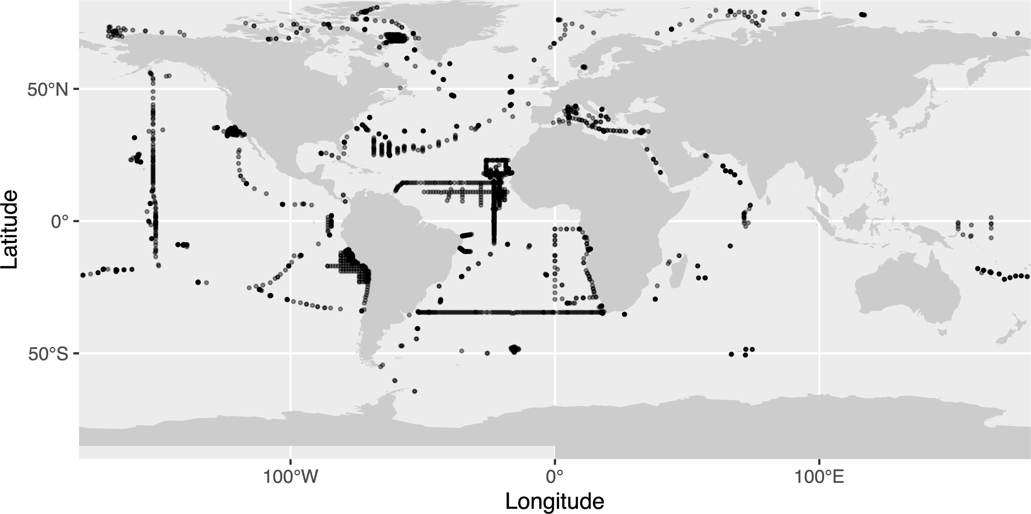
Figure 1 Map of the UVP5 dataset used in this study. Transparency was used to illustrate the density of points on the map.

2.1.2 Image Classification and Size Range Covered

Living organisms were separated from detritus (aggregates, fibers, fecal pellets) as well as artifacts (e.g. bubbles) and classified according to their taxonomic identity. Recognition and sorting of organisms can be a source of bias depending on the levels of perception and experience of the people who perform them. Several cognitive factors biases such as boredom, fatigue or a classification biased towards the most used groups have been presented by Culverhouse (2007) and Culverhouse et al. (2014). To reduce the risk of poor identification, a shared UVP5 taxonomic guide was used to homogenize image sorting into 119 taxonomic groups. The image data were thereafter grouped into 25 broader taxonomic groups (Table S1), and a subset of the resulting dataset was checked for homogeneity of sorting within these groups. A minimum of 51 images and a maximum of 10% of all images were extracted from each group and were independently checked after the assembly of the final data set. The maximum error or uncertainty rate per taxon was 9.8% and a vast majority of taxa were under 2.5%. We checked the classification and if accuracy was <95%, we rechecked the categories to assure proper sorting. In addition, only fully validated profiles were used for this analysis. The resulting global data set consisted of 466,872 images from 3,549 stations. Under-sampled groups with less than 500 images in the dataset which could not be used for a global study were not included in the analysis.

We computed the organisms’ size spectrum to detect the size range within which the UVP5 can be used to properly quantify their distribution. The concentration of objects in the ocean is expected to decrease with size; when this is computed as a normalized size spectrum, the relationship is expected to be linear (Forest et al., 2012). A peak in the size spectrum at the lower size range generally reflects the minimum size of efficient detection by in situ imaging while high variability in the large size range reflects the poor ability to detect rare large objects (Stemmann and Boss, 2012). With that in mind, the spectrum was linear for the size range 1.02-50 mm and organisms outside this range were not included in the analysis since large mobile fauna (including large crustaceans) are likely to be undersampled and small zooplankton organisms close to the UVP5’s threshold of detection are difficult to identify. This size range selection ensures that the data used in this study was properly quantified by the UVP5.

2.1.3 Individual Biomass Estimation

To avoid errors due to incorrect ellipse fits (around appendages of organisms rather than their body, ellipse fitted to non-ellipsoidal organisms, etc.), we chose the spheroid method: it is based on the area (Table 1), which is more consistently measured by the image analysis performed in ZooProcess.

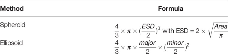
Table 1 Methods of calculating individual biovolume with area (mm2); ESD, the equivalent spherical diameter equivalent (mm); major, the major axis (mm) of the best fit ellipse; minor, the minor axis (mm) of the most suitable ellipse.

For Rhizaria, biovolume (mm³) to carbon (mgC) conversions were done using factors from the literature (Figure S1 and Table S2). For other groups, the conversion from individual volume to individual wet weight assumed a density of 1 g cm^-3 (Kiørboe, 2013). Then the conversion from individual wet weight to individual biomass in carbon units (mgC) was calculated using taxon-specific linear conversion factors from McConville et al. (2016); when several conversion factors were available for a taxon, their median was used for each group. To take into account differences in density of some parts of the organisms, the Appendicularia group was actually split into Appendicularia_body and Appendicularia_house, whereby the “body” group contains images with only the animal and the “house” group contains the house and the animal. For the images labeled Appendicularia_house, we used the relationship of house diameter (major axis) to Appendicularia trunk length from Lombard and Kiørboe (2010). We then converted this body size equivalent into carbon weight using the corresponding relationship from Lombard et al. (2009). For the images labeled Appendicularia_body, we converted the biovolume of the organism into carbon weight using the corresponding relationship from Lombard et al. (2009). Two groups also have been created to separate the Collodaria into solitary Collodaria and colonial Collodaria. This choice was done based on the fact that solitary Collodaria are smaller than colonial ones and have a different vertical distribution (Faillettaz et al., 2016). For solitary collodarians with a dark central capsule (subgroup of solitary Collodaria) described in Biard et al. (2016), the estimation of carbon (0.189 mgC mm^-3) by Mansour et al. (2021) was done on the capsule of the organisms. As Zooprocess measures the area of the whole organism, we determined the ratio $\frac{area whole organism}{area central capsule}=0.713$ and applied this factor to avoid overestimation of carbon biomass for this group. For the rest of the collodarians, the estimation of Mansour et al. (2021) was directly applied.

2.2 Environmental Data Collection and Processing

In order to develop relationships between regional characteristics of the environment (Figures S2–4) and observed biomass, climatologies from the World Ocean Atlas (WOA) (Garcia et al., 2019) were used for temperature (in °C), salinity, oxygen (converted from μmol kg^-1 to kPa for better physiological interpretation), and macronutrients (nitrate, phosphate and silicate in μmol kg^-1). We selected the data sets defined on a 1° horizontal grid, over the 0-500 m depth range, and with a monthly temporal resolution. Temporal coverage was from 2005 to 2017 for salinity and temperature and 1955 to 2017 for the other variables. We also used monthly averaged surface chlorophyll-a data (Chl a in mg m^-3) resolved to 1/24° from 2005 to 2017 from the Copernicus database (OCEANCOLOUR_GLO_CHL_L4_REP_OBSERVATIONS_009_082) as well as bathymetry data from NOAA (Amante and Eakins, 2009) with a spatial resolution of 10 minutes; both were re-gridded to a 1° grid. Finally, distance to coast was computed by calculating the distance of all 1°×1° cells to the closest cell associated to land using the raster package (Hijmans, 2021). To obtain annual climatologies, when relevant, each monthly variable was averaged over its time period of coverage.

This environmental data was then matched to the UVP5 data on the 1°×1° grid. Since the 1°x1° grid used by WOA does not necessarily follow the contour line of the coast perfectly, some UVP5 profiles could not be directly matched to the environmental grids. This is mostly the case where e.g. the coast is situated in a 45 degree angle to latitude or longitude, thereby creating triangle shaped areas that are not covered by the rectangular grid. For profiles that lie in such corners of the grid, we used the environmental values of the closest neighboring 1°×1° WOA cell. In the epipelagic world model, 3,002 points did have a direct match while 156 points did not have a direct match. Out of these 156 points, 14 were not in a neighboring 1°×1° WOA cell and were removed from the model input. For the mesopelagic, 2,172 did have a direct match, while 104 points had a match in a neighboring grid cell and 2 points did not and were removed from the model input. Maps that show the close vicinity of non-matching points to adjacent WOA cells are shown in Supplementary Figure 5.

To assess whether we are able to describe various environmental conditions with the UVP5 samples, we compared the distributions of each variable in the worldwide WOA dataset and in the subset matched to UVP5 profiles (Figures S6, S7). Although the geographical coverage is not homogeneous (Figure 1), the coverage of environmental conditions is good and warrants the use of habitat models.

2.3 Habitat Modeling

The steps of this process are summarized in Figure 2.

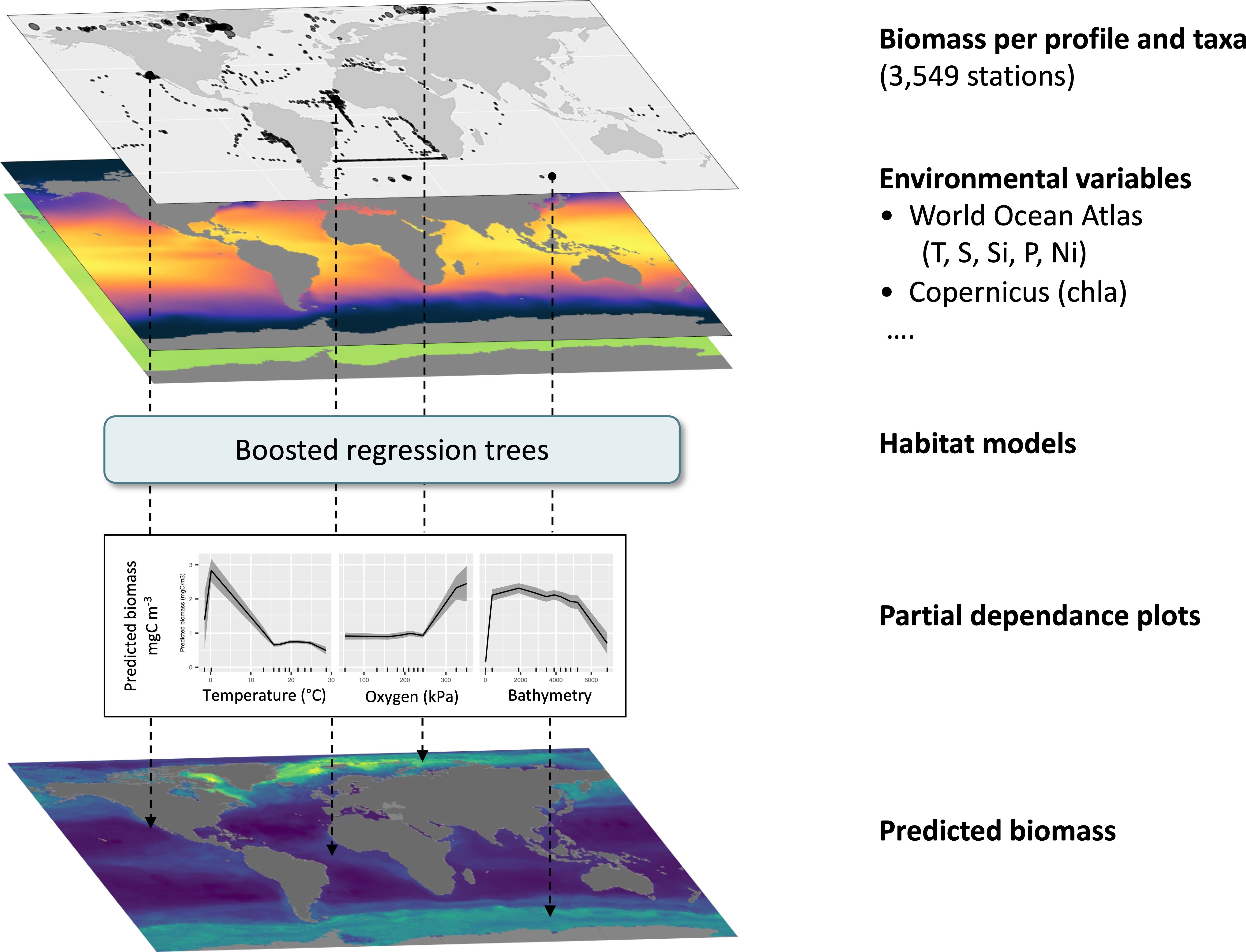
Figure 2 Methodology followed from data selection to prediction of global biomass.

2.3.1 Modeling Tools

In this work we used boosted regression trees (BRTs) to predict the biomass of different zooplankton groups as they show different advantages over other commonly used machine learning approaches for the nature of our dataset and intended application (Elith and Graham, 2009). This ensemble method uses regression trees, models that link a response (here biomass) to predictors (environmental variables) by successive dichotomous separations (Breiman et al., 1984; Hastie et al., 2001). Regression trees automatically select the relevant explanatory variables, can deal with categorical or continuous inputs, are not sensitive to the distribution of the continuous ones, can represent relations of arbitrary form and naturally include interactions among explanatory variables (Elith et al., 2006). With so-called surrogate splits, they can also deal with missing values in the explanatory variables. They are therefore very convenient to use, but their predictive power is often limited and they have difficulties to capture smooth relationships. Boosting is a way to overcome these drawbacks (Schapire, 2003). It is based on the fact that it is easier to find many rough rules of thumb than to find a single, highly accurate prediction rule (Schapire, 2003). BRTs combine many short regression trees in succession, each new tree being adjusted to consider the observations poorly predicted by the previous ones (Elith et al., 2006; Leathwick et al., 2006; Elith et al., 2008). This improves predictive performance and the smoothness of the prediction (Leathwick et al., 2006). In addition, only a random subset of the input data is used to fit each tree and this stochastic component reduces the variance of the final model ensemble (Friedman, 2002).

Boosted regression trees (BRTs) have an ability to handle a large number of variables and - other than Generalised Linear Models (GLMs, Nelder and Wedderburn (1972)) or Generalised Additive Models (GAMs, Hastie and Tibshirani (1986); De’ath (2007); Elith et al. (2008)) - do not seek to fit one single model portraying the relationship of the response variable (here biomass) and its predictors (environmental variables). Various recent studies (González Carman et al., 2019; Chen et al., 2020; Hu et al., 2021) have compared BRTs results to other modeling tools such as GAMs, GLMs, Random Forests (RFs), Maximum Entropy modeling (Phillips et al., 2006; Elith and Graham, 2009) or neural networks and have obtained better predictive performance with BRTs. Other studies (Zhang et al., 2018; Son et al., 2018) used complementary GAMs and BRTs to study the effects of explanatory variables. However, BRTs could be slower than RFs (Chen et al., 2020) and training parameters need to be chosen carefully to avoid overfitting (Leathwick et al., 2006; Elith and Graham, 2009). BRTs were chosen over RFs because of their capacity to reduce both the bias and the variance of model results (Hastie et al., 2001). BRTs are also less sensitive to the effect of extreme outliers and the inclusion of irrelevant predictors (Leathwick et al., 2006). This makes them suitable for plankton datasets, as sometimes very high plankton biomass values do occur during blooms (Brodeur et al., 2018; Pettitt-Wade et al., 2020). BRTs also have the ability to handle sharp discontinuities which is not the case of the GAMs (Elith et al., 2008). This is important when modeling taxa which can have a narrow habitat.

In addition, in regression trees, the loss function, used to determine which dichotomous split to perform, can be changed to be adapted to the distribution of residuals. Here we explored the classic mean squared error, which assumed a somewhat normal distribution of the residuals, as well as a Tweedie loss adapted to zero-inflated data (Zhou et al., 2019), and a Poissonian loss, which considered data as discrete counts, also including many zeros. To use the Poisson loss, the biomass was scaled so that the value of the 1% quantile was ≥ 1 and then rounded to the nearest integer; the inverse scaling was performed after prediction. This later approach proved to produce the best fits and more robust models in a few test taxa and all models were therefore fitted with Poisson loss. The models and statistics were computed using the xgboost package (Chen et al., 2021) in R version 4.1.2 (R Core Team, 2021).

2.3.2 Spatial Partitioning of the Data

Individual biomass values derived from UVP5 images and environmental data measured at various layers were both averaged over a depth range of interest and matched geographically, on the 1°×1° grid. Biomass values matched to the same 1° pixel, and therefore associated to exactly the same environmental data, were averaged.

We hypothesized that an association between biomass and environment investigated at a fine scale could be more efficiently learned by the model because is contains less noise, so we divided the data vertically between the epipelagic (0-200 m) and mesopelagic (200-500 m) zones and also tried a finer partition, into 100 m depth bins between 0 and 500 m. Evaluating separate models for each layer could allow to focus on finer subgroups within our quite coarse taxonomic units (some species being mostly present in one of the layers) and therefore define biomass-habitat relationships at a finer, more relevant biological level.

For the same reason, we also built models on subsets of data partitioned geographically. Indeed, polar copepods have a different thermal niche compared to tropical ones (Rombouts et al., 2009; McGinty et al., 2021). So, in addition to a model fitted on the global dataset (world), we trained models on data from the region between 40°S and 40°N (low latitude) and from the data collected outside of this latitudinal band (high latitude). Out of the 3,549 profiles composing the UVP5 dataset, 2,837 are located between 40°S and 40°N and 712 were done outside of this latitudinal band.

2.3.3 Data Splits for Model Training, Assessment and Evaluation

For each taxon in each spatial partition, the data was split to distribute 80% of it in a training and validation sets, on which the model was fitted and assessed, and 20% to a test set, on which predictive performance was evaluated. This split was stratified according to the deciles of biomass in the data, to ensure that both the learning and test sets contained low and high biomass points.

To choose model hyperparameters (i.e. parameters of the model adjustment algorithm) and to evaluate the variability in the prediction due to the constitution of the training set, each 80% portion set was resampled through five-fold cross validation repeated 20 times [i.e. 100 resamples; (Hastie et al., 2001)]. For each cross-validation fold, the model was actually trained on four folds and validated on the last one. The splits into the five folds were also stratified according to the deciles of biomass, for the same reason invoked above.

2.3.4 Selection of Hyperparameters and Model Evaluation

To extract as much information from the data, while avoiding overfitting, various combinations of hyperparameters were tested for each model (Elith et al., 2006). They included: 1) the learning rate per tree determining the contribution of each tree to the ensemble model (0.05, 0.08 and 0.1 were tested); 2) the maximum depth of a tree (2, 4 and 8 were tested); 3) the minimum number of elements per leaf (which also limits the depth of the trees; 1, 3 and 5 were used); 4) the number of trees used for the prediction (values up to 600 were tested). For each combination, the model was fitted to the training set and evaluated on the validation set of each of the 100 resamples; the loss was then averaged over the 100 resamples. The best set of hyperparameters is usually the one for which this average loss is minimal. The differences around that minimum are often small and not always meaningful; to be sure to avoid overfitting, we applied an early stopping criterion whereby the increase in the number of trees was stopped when the error did not decrease by more than 1% after adding 10 trees.

Once the best set of hyperparameters had been chosen, the relevance of the corresponding model was quantified by the Pearson correlation between the observed biomass data in the test set and the predicted biomass, where prediction is the average of the predictions of the 100 models fitted to the resamples. This metric captures the model’s ability to correctly represent general trends and patterns in the data set and is one way to compute the R². The significance of this correlation can also be tested and quantified with a p-value. These metrics can be readily compared across the various spatial partitions of the data because they represent the skill of the models on an independent data set, not the quality of the fit to the training data (like the way the R² is usually computed). To compare the worldwide and regional approaches fairly, it is important to focus on the same regional subset. To this effect, two additional R² were computed for the global model: on the test data located inside the 40°S-40°N latitudinal band and on those outside of it (world low latitude and world high latitude).

2.3.5 Effect of Environmental Variables

To identify which environmental variables drive the change of biomass in each specific model, the percentage of variance explained by each variable was calculated as the sum of the effects of the variable at each node of each tree where it was used. To describe the shape of the effect of each variable, univariate partial dependence plots were computed as the average ± standard deviation marginal effect of the variable in the 100 resamples. Practically, the variable of interest was set at a given value at all training points, the other variables were left at their original values, the average biomass predicted over all points was computed, for each resample; then the mean and standard deviation of those averages were computed across resamples. Finally, the variable was set to another value and so on. To describe the full range of each variable, the partial dependence was estimated at 10% quantile.

2.3.6 Extrapolation to the Globe

To obtain global maps of predicted biomass, the regression between UVP5 biomass data and environmental variables was applied to all points in the corresponding partition of the world, in depth and space. Because 100 models were fitted to the resamples of the training data, the standard deviation of biomass among the 100 predictions (σ_b) can be computed in addition to the mean (m_b), and the coefficient of variation (CV), defined as $CV=\frac{{\sigma }_b}{m_b}$, then gives an indication of the uncertainty of the model predictions.

To get a robust estimate of global zooplankton biomass in the 1.02 mm to 50 mm size range, we chose to be conservative (i.e. ad minima): only the taxonomic groups in the global partition for which the correlation between predicted and observed biomass was significant were used. The surface area of each 1°×1° cell was computed using the following formula:

with the area A in m², the south and north latitudinal limits of the cell in radians and ℛ, the earth radius (6,378.137 km). For each group used, the biomass was integrated over the relevant layer in each 1°×1° cell by the following calculation

where $\widehat{b}$ is the estimated biomass in mgC.m^-3, A in m² is defined above, l is the layer thickness in m and therefore ${\widehat{b}}_t$ is the total biomass in mgC. Finally, the global ad minima zooplankton biomass estimate was computed by adding up the biomass for all selected groups and the 0-200 and 200-500 m depth layer.

3 Results

3.1 Model Comparison

We estimated model performance on the worldwide UVP5 dataset and on a spatial partition of the dataset in low (inside 40°N and 40°S) and high latitudes (outside of the 40°N-40°S latitudinal band) as well as on different depth layers. We hypothesized that a finer data selection might enable the respective model to learn the regional or depth specific habitat more appropriately. Yet, this also meant fitting models to fewer data points. In the end, we find that no clear trend emerges from the relevant comparisons (Figure 3): global models are better in 13 comparisons and partitioned models are better in 14 comparisons, whereas for 11 comparisons no clear decision can be made. Comparisons can only be made within a given depth layer between the same regional partitions (e.g. world low latitude only containing the data predicted by the global model between 40°N-40°S vs low latitude; world high latitude only containing data north of 40°N and south of 40°S from the global model vs high latitude).

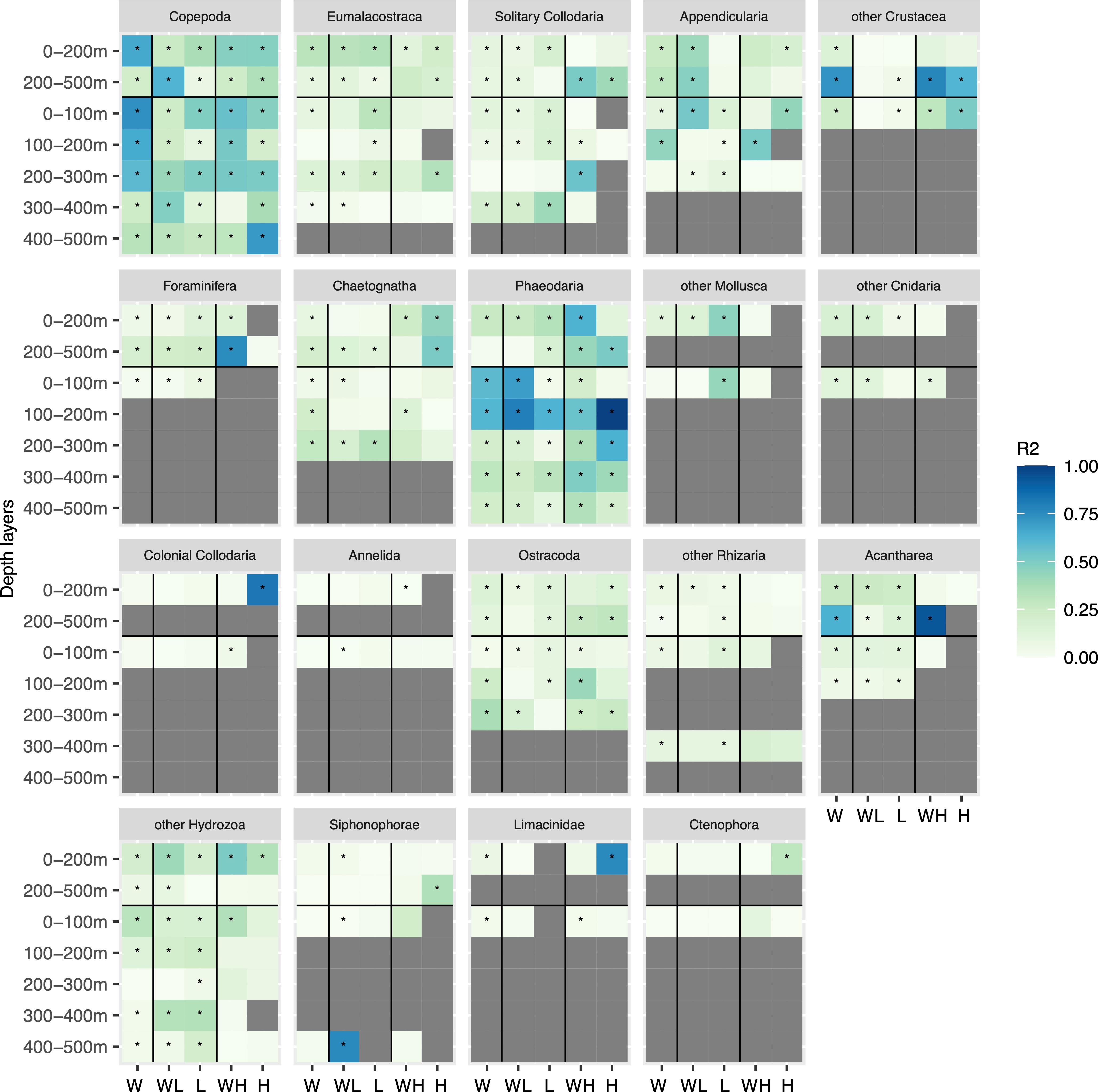
Figure 3 Heatmap of the models’ R² between observed and predicted biomass for all zooplankton groups arranged from the most important in terms of biomass (Copepoda) to the least important (Limacinidae) in the different depth layers. The regions correspond to: W for world (model run on all data); WL for world low (data between 40°N and 40°S from the world model); L for low latitude (model run between 40°N and 40°S); WH for world high (data outside of 40N and 40S from the world model); H for high latitude (model run outside of 40°N and 40°S). The stars indicate significant results (p-value < 0.05) obtained with the Pearson correlation test.

For some groups such as Annelida and some Mollusca, the high latitude model could not be computed (symbolized by a grey cell) either because they were considered as rare (< 500 images in the layer modeled) or because the model could not learn the link between biomass and environment for this group. However, for other taxa such as Copepoda, solitary Collodaria or Phaeodaria, high and low latitude models are generally better than the world model, as indicated by a higher R² value (Figure 3). In the epipelagic layer, for Copepoda, the R² of world low latitude is 0.26 vs 0.37 in the low latitude model. For the mesopelagic, low latitude has an R² of 0.07, lower than the one for world low latitude (0.62). For Appendicularia in the epipelagic layer, the best R² values are obtained in the world low latitude (0.41) and world high latitude (0.24) models respectively compared to low latitude (0.01) and high latitude (0.19).

As for the vertical 100 m-bin layers partition, we obtained the best results overall with the global model. The finer vertical definition also gives better results for multiple other groups such as Appendicularia, Phaeodaria and Ostracoda between 0 and 300 m. In most cases, only the top 100 m layer model worked for this 100 m vertical partition. Overall, the most consistently good choice, when considering all taxa, is a worldwide model fitted separately to the epipelagic (0-200 m) and mesopelagic (200-500 m) layers. This is therefore the configuration retained for the total, global biomass estimate. In Figure 3, taxa are arranged in decreasing order of global biomass in the epipelagic layer. For the top five taxa [Copepoda (R² = 0.66), Eumalacostraca (R² = 0.31), solitary Collodaria (R² = 0.10), Appendicularia (R² = 0.26) and other Crustacea (R² = 0.15)], the correlation between true and predicted biomass is significant (p-value < 0.05) in the epipelagic worldwide model. In the mesopelagic layer, the correlations for all five groups are also significant (p-value < 0.05 with respective R² of 0.22, 0.10, 0.09, 0.30 and 0.72).

3.2 Group-Wise Contribution to Global Zooplankton Biomass

Figure 4 shows the biomass per group predicted for the three spatial partitions and divided into the epi- (0-200 m) and mesopelagic (200-500 m) layers. For the worldwide model, the dominant groups in terms of biomass in the epipelagic were Copepoda (0.083 ± 0.020 PgC), Eumalacostraca (0.058 ± 0.017 PgC) and solitary Collodaria (0.038 ± 0.008 PgC) (Figure 4). Among the groups displaying a significant correlation (p-value < 0.05) between true and predicted biomass (and therefore retained for the global estimate), crustaceans (Copepoda, Eumalacostraca, other Crustacea and Ostracoda) represented 68.4% (0.157 PgC) of the biomass in this layer; Rhizaria (solitary Collodaria, Foraminifera, Phaeodaria, other Rhizaria and Acantharea) made up 20.6% (0.047 PgC); but the Cnidaria (other Cnidaria and other Hydrozoa) represented only 0.56% of the global zooplankton biomass (0.0013 PgC). In other words, Crustacea and Rhizaria together made up ~89.1% of the biomass predicted in the epipelagic layer. In the deeper mesopelagic layer, Copepoda (0.061 ± 0.016 PgC) were still the dominant group in terms of biomass, followed by Eumalacostraca (0.049 ± 0.014 PgC) and other Crustaceans (0.017 ± 0.001 PgC) combined. Crustacea (Copepoda, Eumalacostaca, other Crustacea and Ostracoda) represented 0.129 PgC, equivalent to 74.4% of this layer’s biomass, while Rhizaria (Foraminifera, solitary Collodaria, other Rhizaria and Acantharea) totaled 0.014 PgC, representing 10.1%, equivalent to most of the remaining biomass in the layer. When combining the results from these two layers, Copepoda represented 44.4% of the global integrated biomass, followed by Eumalacostraca (15.6%), solitary Collodaria (13.1%) and other Crustacea (11.2%). More broadly, Crustacea (Copepoda, Eumalacostraca, other Crustacea and Ostracoda) represented 0.222 PgC or 71.3% of the biomass predicted over 0-500 m, while Rhizaria (Foraminifera, solitary Collodaria, other Rhizaria and Acantharea) made up 0.019 PgC or 10.8% of biomass.

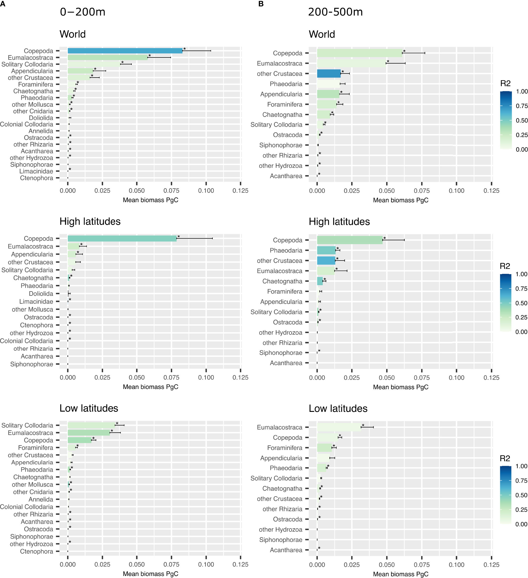
Figure 4 Barplots showing the mean biomass predicted in PgC at 0-200 m (A) and 200-500 m (B) depth for each group ranked from highest to lowest biomass in 3 types of models: world, outside 40°N-40°S and inside 40°N-40°S. Error bars correspond to upper interval of the biomass estimation’s standard deviation. The stars indicate a significant result (p-value < 0.05) obtained with the Pearson correlation test.

Copepoda were particularly dominant in high latitudes, especially in the epipelagic layer. In the low latitude model, solitary Collodaria contributed most in the epipelagic, followed by Eumalacostraca, Copepoda and Foraminifera. Eumalacostraca dominated biomass in the mesopelagic layer in low latitudes followed by Copepoda and Foraminifera.

3.3 Spatial Distribution Patterns and Occupied Habitat

Presenting the global distribution patterns of all zooplankton groups is beyond the scope of this paper. Instead, we focus on the results for the three groups contributing most to the total global biomass (Copepoda, Eumalacostraca and Solitary Collodaria) as well as on Phaeodaria and Acantharea, Rhizarians that were shown to be important contributors to zooplankton biomass that are underestimated by net-based sampling (Biard et al., 2016). The predicted fields for all modeled groups will be made available in the GitHub repository linked in the data availability statement upon publication of the article.

3.3.1 Copepoda

Copepoda is one of the best predicted groups in the epipelagic (R² = 0.66), likely because it is the most abundant. The structuring environmental variables were different for the epi- (Figures S8A, B) and mesopelagic layers (Figures S8C, D): temperature (33%) and oxygen (19%) for the former and temperature (29%), bathymetry (19%) and chlorophyll a (15%) for the latter. The highest copepod biomass in the top 200m was found in high latitudes (Figure 5A), where water temperature is low and oxygen concentrations are relatively high. In the mesopelagic layer (Figure 5B), high copepod biomass was associated with shallow coastal and cold water masses. The patterns of distribution predicted by the global models were similar in both layers (Figures 5A, B), with the highest predicted biomass values in the Baffin Bay, Labrador Sea and Greenland Sea as well as at the Southern Ocean polar front region. The lowest predicted biomass was predicted at oceanic gyres and in the Arctic, north of 80°N. For both layers, the highest values of the coefficient of variation (Figure 5C) were found north of Canada and Greenland, as well as south of 60°S, especially for the epipelagic layer. These high values depict disagreement among the 100 models fitted to the data resamples and therefore inform on the uncertainty of the model in these zones. Caution is therefore advised regarding the interpretation of the very low values of biomass predicted in those regions. In the northern hemisphere, except for the Arctic ocean, the values of the coefficient of variation were rather low at locations where either low or high biomass values were predicted. In the southern hemisphere, model predictions varied relatively strongly at the level of the Antarctic polar front (Figures 5C, D).

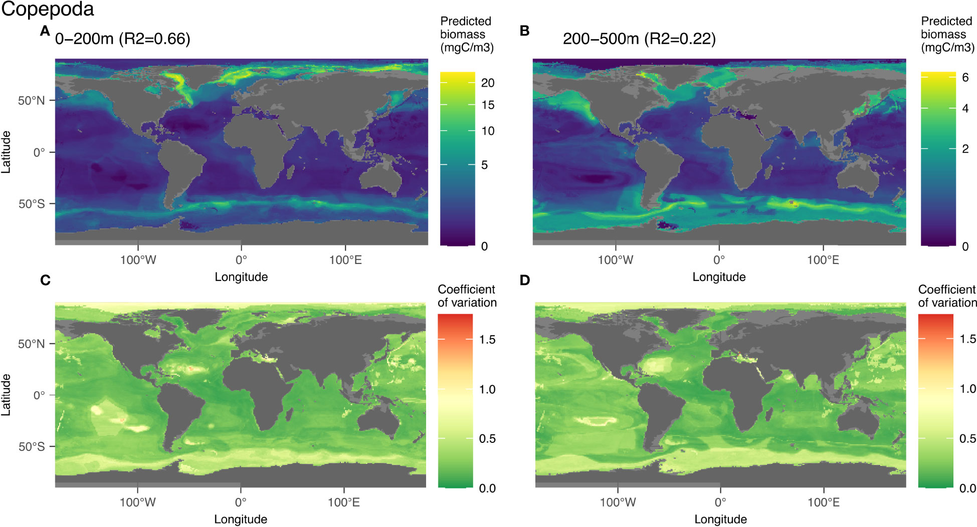
Figure 5 Map of the mean biomass (color scale is log-transformed) of Copepoda as predicted by the model on 0-200 m (A) 200-500 m data (B) as well as the coefficient of variation for the 0-200 m model (C) and 200-500 m one (D). The color scale for the coefficient of variation has the same range for Figures 5–9.

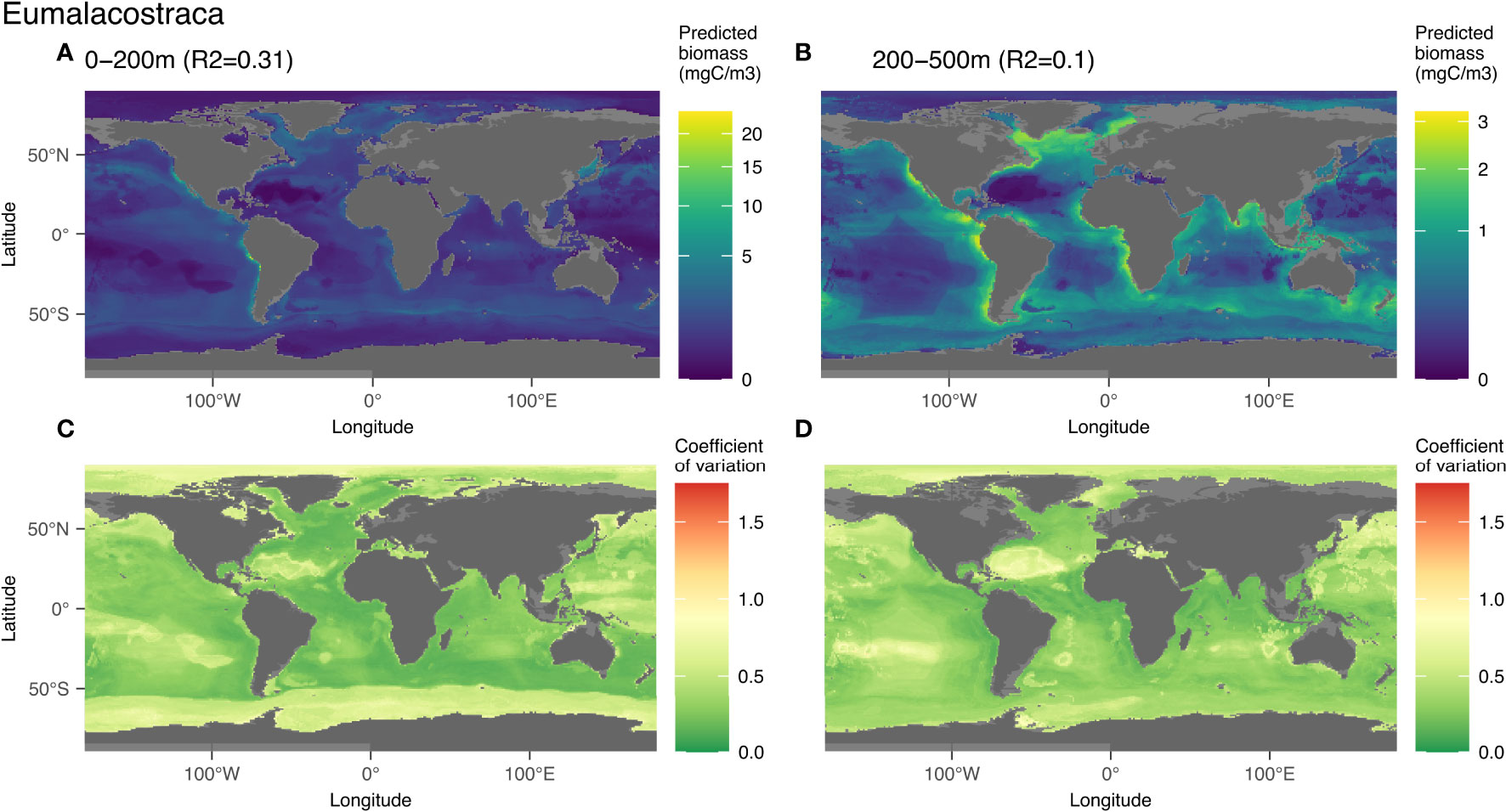
Figure 6 Map of the mean biomass (color scale is log-transformed) of Copepoda as predicted by the model on 0-200 m (A) 200-500 m data (B) as well as the coefficient of variation for the 0-200 m model (C) and 200-500 m one (D). The color scale for the coefficient of variation has the same range for Figures 5–9.

3.3.2 Eumalacostraca

Eumalacostraca contains mostly vignettes of euphausiids, amphipods and decapods. They were predicted globally with an R² of 0.31 for the epi- and 0.1 for the mesopelagic layer, both with significant p-values (p-value < 0.05; Figure 3). In the epipelagic, high biomass of these organisms was associated with high concentrations of phosphate (22%) and low concentrations of silicate (17%) (Figures S9A, B). In the mesopelagic layer, the distribution of this group was associated with low concentrations of silicate (16%), bathymetry (15%) and high chlorophyll α (15%) (Figures S9C, D). In terms of spatial distribution, high biomass is predicted in eastern boundary currents, especially in the Peruvian and Californian upwelling systems. Low biomass is predicted in high latitudes and in the oceanic gyres, especially in the North Atlantic. Similar patterns were predicted in the mesopelagic layer, but with lower biomass values. The model uncertainties are highest in the zones of low biomass (high latitudes and oceanic gyres).

3.3.3 Solitary Collodaria

Solitary Collodaria were predicted globally with an R² of 0.1 for the epi- and 0.09 for the mesopelagic layer, both with significant p-values (p-value < 0.05; Figure 3). In the epipelagic, the distribution of solitary Collodaria were mainly associated with low salinity (21%, between 35 and 37) and bathymetry (14%) (Figures S10A, B). In the mesopelagic, high abundances of this group were associated with distance to shore (18%) and high chlorophyll a (17%)(Figures S10C, D). In this layer, 65% of the biomass was predicted at less than 1,000 km from the coast. Solitary collodaria were mainly located between 50°N and 50°S, in a rather diffuse manner (Figure 7) with maximum biomass predicted at the equator. In the intertropical region, the highest biomass was found in the epipelagic zones of productive areas such as the upwelling regions off the western coast of Africa (Cape Verde and Angola) and of the eastern boundary of the Pacific Ocean (Peru and California). The model also predicted high biomass in the Mediterranean Sea. The importance of the environmental variable “distance to coast” in the learning process created unusual patterns in the prediction map such as a hexagonal shape in the Pacific Ocean. North of 50°N and south of 50°S, environments that are typically characterized by water masses with low salinity (1^st most structuring variable in the epipelagic) and high nitrate (4^th variable), the predicted biomass was rather low especially in the epipelagic layer.

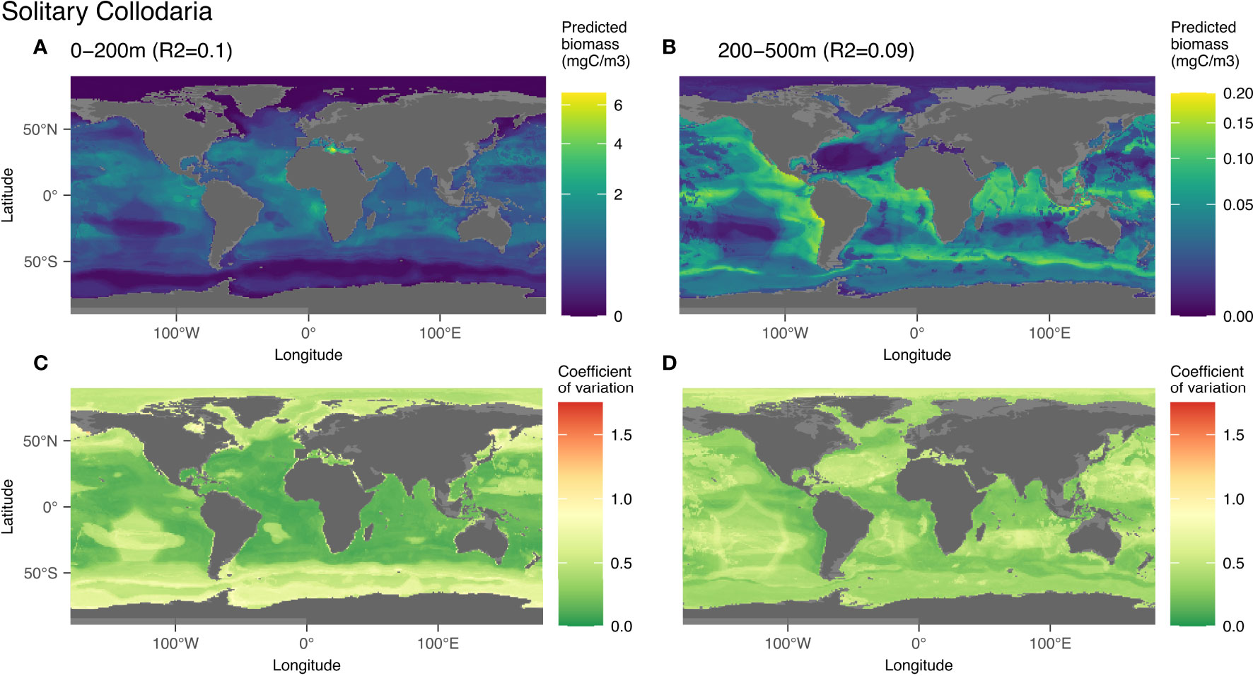
Figure 7 Map of the mean biomass (color scale is log-transformed) of solitary Collodaria as predicted by themodel on 0-200 m (A) 200-500 m data (B) as well as the coefficient of variation for the 0-200 m model (C) and 200-500 m one (D). The color scale for the coefficient of variation has the same range for Figures 5–9.

3.3.4 Phaeodaria

For this group, the worldwide epipelagic model was statistically significant (p-value < 0.05; Figure 8) with an R² of 0.27, but the mesopelagic model was not (p-value > 0.05; Figure 3). Therefore, only the 0-200 m layer is displayed (Figure 8). In this layer, Phaeodaria was one of the best predicted groups (Figure 3) especially in the upper 200m. The predicted epipelagic distribution of Phaeodaria is associated with low values of salinity (38%) followed by bathymetry (11%), surface chlorophyll a (10%), oxygen and temperature (8% each) (Figures S11A, B). This is visualised on the map of global prediction (Figure 8A) on which high biomass was mainly predicted in the Californian upwelling (characterized by low salinity, cold and coastal waters), with lower biomass north of the upwelling up to the Gulf of Alaska. High biomass values were also predicted in the Bay of Bengal and Adaman Sea. The coefficient of variation in zones of high biomass is very low, providing strong confidence in this pattern. The lowest predicted biomass for this group are found in oceanic gyres and high latitudes of the northern hemisphere.

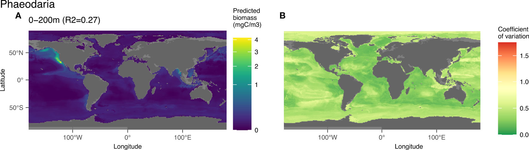
Figure 8 Map of the mean biomass (color scale is log-transformed) of Phaeodaria as predicted by the model on 0-200 m (A), as well as the coefficient of variation for the 0-200 m model (B). In the map of predicted biomass, 12 cells in the California upwelling presented a value between 3 and 6 mgC m^-3 and were represented here in yellow to observe the distribution of this group on a global scale. The color scale for the coefficient of variation has the same range for Figures 5–9.

3.3.5 Acantharea

The group Acantharea was predicted with low total biomass (Figure 4). This group was well predicted in the world model fitted with the epi- (R² = 0.26) and mesopelagic (R² = 0.63) layers (Figure 9). In the epipelagic layer, nitrate (18%), salinity (15%) and phosphate (12%) were the main driving variables (Figures S12A, B). In the mesopelagic layer, the link between biomass and environment (Figure 9B) was defined by the influence of several variables: silicate (19%), phosphate (12%) followed by chlorophyll a (12%) (Figures S12C, D). The highest epipelagic biomass (Figure 9A) was predicted in the intertropical range, in productive areas such as the upwellings off the West coast of Africa (Cape Verde, Angola) and America (Peru and California). These high biomass patches are associated with a salinity around 35 as the 2^nd most structuring variable, as well as with high nitrate and phosphate concentrations (respectively 1^st and 3^rd). Intermediate biomass values were predicted mostly between 50°N and 50°S in a diffuse way, except in the oceanic gyres where the predicted biomass was lowest. The largest uncertainty was present in the Southern and Artic Oceans, Bering Sea and Gulf of Alaska where low biomass values were predicted (Figure 9C). In the mesopelagic layer, biomass was predicted to be 16.7-times lower overall (Figure 9B), with highest values found in the Gulf of Alaska and the Bering Sea. Intermediate biomass values were predicted for the upwelling regions and the Southern Ocean. In this layer, the high biomass estimates correspond with low coefficient of variation values (Figure 9D).

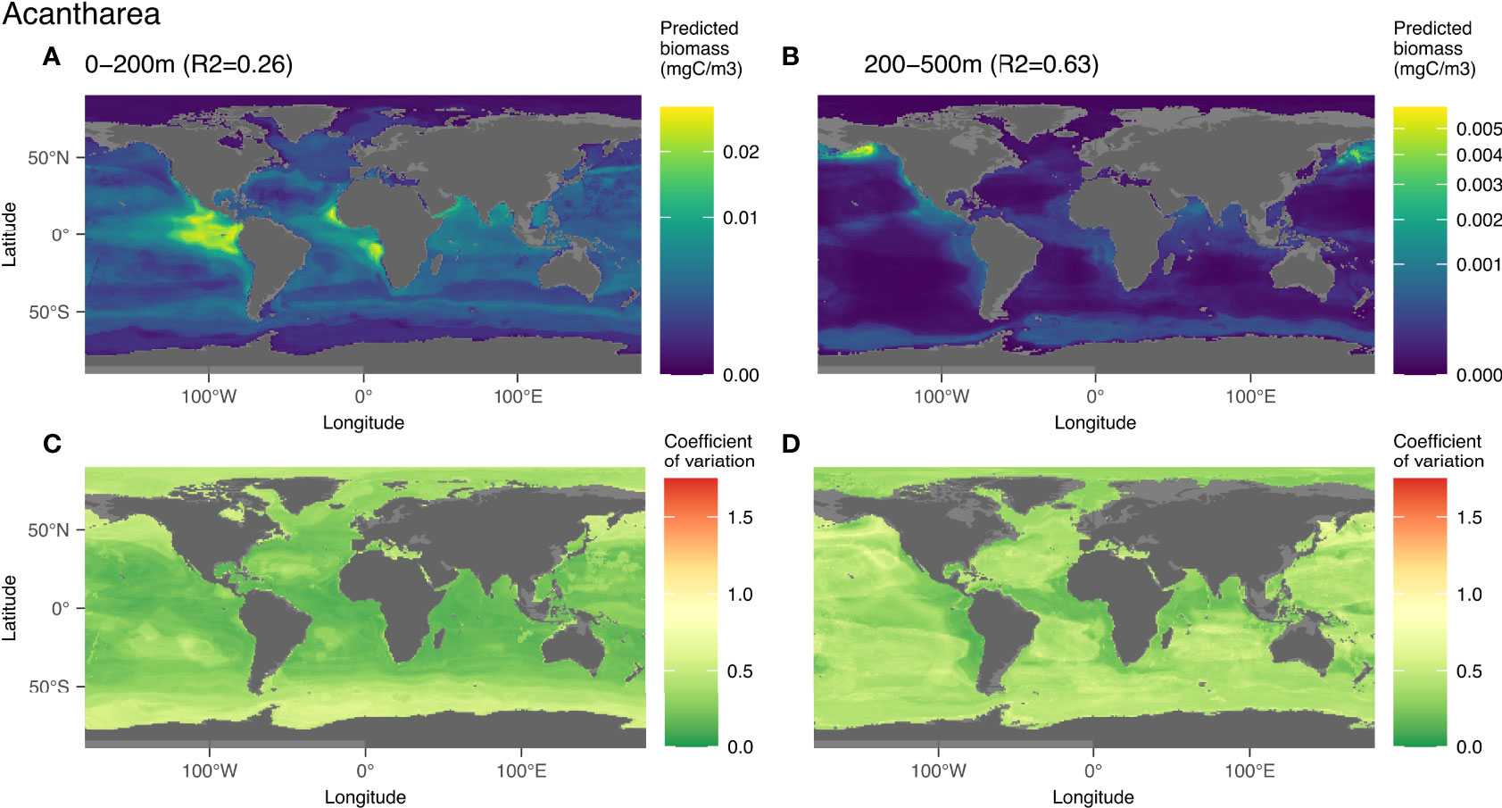
Figure 9 Map of the mean biomass (color scale is log-transformed) of Acantharea as predicted by the model on 0-200 m (A), 200-500 m data (B), as well as the coefficient of variation for the 0-200 m model (C) and 200-500 m one (D). The color scale for the coefficient of variation has the same range for Figures 5–9.

3.4 In Situ Imaging Compared to Net Based Sampling

The latitudinal biomass distribution of Copepoda and Rhizaria obtained by combining the predictions of global models for the epi- and mesopelagic is shown in Figure 10. It is compared against data (interpolated on 0-500 m) from the Tara Oceans mission (Pesant et al., 2015; Soviadan et al., 2022) acquired using 300 μm multinet samples and ZooScan (Gorsky et al., 2010). To make the comparison meaningful, we only selected organisms in the ZooScan samples with an ESD >1 mm. For Copepoda, the values observed by the UVP5 and the nets reveal a similar latitudinal pattern between 70°N and 60°S. The trend computed on the output of the models shows lower biomass between 40°N and 40°S compared to Tara observations. For Rhizaria, the highest biomass was found in the UVP5 observations and models around the equator. Generally, almost no Rhizaria were observed in nets whereas they were consistently observed with the UVP5.

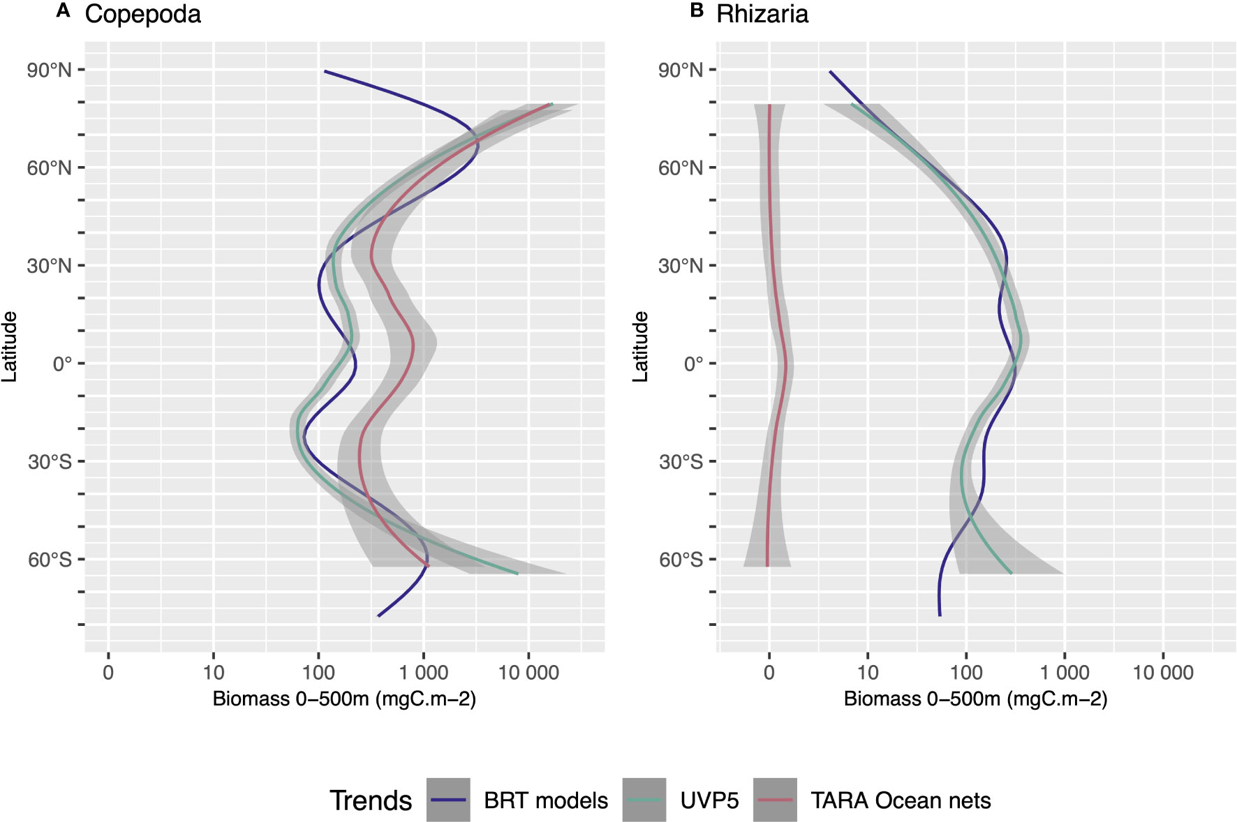
Figure 10 Comparison of the latitudinal distribution of biomass mgC m^-2) integrated over 0-500m depth between our models’ estimation and the results from the Tara Ocean multinet (300 mm mesh size), for Copepoda (A) and Rhizaria (B). Trends were obtained by using Loess regression on: BRT models (blue line) using the global model outputs for Copepoda or Rhizaria (summed across 0-200 m and 200-500 m depth); UVP5 data (green line) using the biomass as seen by the UVP5 between 0-500m; TARA Ocean net data (red line) using the sampling points between 0-500m. The Shaded areas represent the 95% confidence interval of the Loess fit.

3.5 Global Zooplankton Biomass Distribution

The biomass integrated over 0-500 m was predicted to be maximal at around 60°N and 55°S, with values decreasing both north and south of these two latitudes (Figure 11). The lowest values of biomass were predicted north of 80°N and in the Weddell Sea as well as in the oceanic gyres (especially in the southern hemisphere). We also observed an increase of the predicted biomass around the equator. The highest biomass values were predicted between 50 and 80°N, in coastal waters of the Labrador Sea and Baffin Bay, as well as in the Greenland Sea. Relatively high biomass was predicted around these locations as well as in the Gulf of Alaska, Bering Sea and Sea of Okhotsk. A band of high biomass was predicted between 40 and 50°S, a region associated with the Arctic polar front.

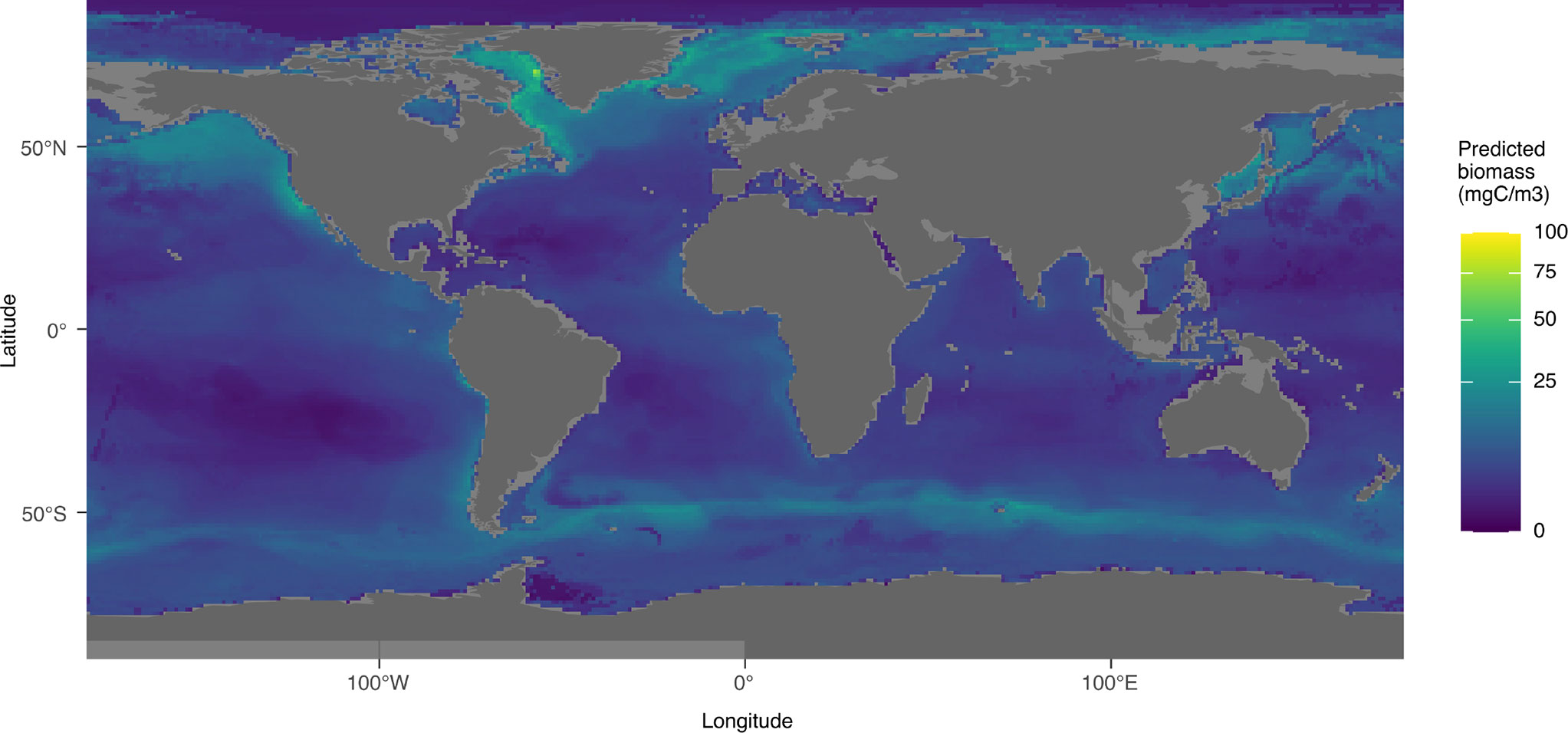
Figure 11 Distribution map of the predicted minimum global biomass between 0 and 500m using taxa which obtained a significant result (p-value < 0.05) in Pearson test between the predicted biomass and the biomass calculated from UVP5 data.

Finally, by summing only the predictions that significantly correlated with observations, we can get to a first robust, conservative, global biomass estimate of zooplankton biomass based on UVP5 in situ imaging. As not all groups could be included in this computation, we refer to the following numbers as biomass ad minima. With that in mind, the zooplankton biomass estimated by the models was 0.229 PgC for the epipelagic, and 0.173 PgC for the mesopelagic. Thus, the estimated biomass for the upper 500m of the ocean is to 0.403 PgC.

4 Discussion

4.1 Sensitivity of Model Prediction to Partitioning

In this study, we explored whether a partitioning approach would improve model performance through the use of different horizontal and vertical divisions of our dataset. The aim of using partitioned models was to test if we could model local taxa that otherwise would be mixed within the coarse taxonomic definition imposed by the dataset. The R² computed on the models’ output show a high variability across groups, layers and regional combinations. Overall, when comparing each partitioned model to the same zone in the global model, the global and the partitioned models had similar performance. The reduction in dataset size might be the explanation why in many cases global models perform better than the smaller partitioned models. The high latitude dataset contains 712 UVP5 profiles, the low latitude 2,837 and the world 3,549 data points. Another drawback of the partitioned models could be that some groups might have an environmental habitat associated with regions on both sides of the limits of the two models (here 40°N or 40°S). A vertical resolution that consists of two layers (0-200 and 200-500m) provided the best results (Figure 3) compared to a finer depth separation. The reduction of data per model with a finer depth layer resolution probably made it impossible for some models to learn the association between a group’s biomass distribution and the associated habitat properties, either because the model could not learn this association or because the group was considered rare (< 500 images). If enough data are available, however, a finer vertical model might perform better, because it better delimits the vertical habitat structure. This seems to be the case for the Phaeodaria for which models with 100 m resolution obtained higher R² results, especially for those between 0 and 300 m depth.

4.2 Group-Wise Contribution to Global Zooplankton Biomass

Globally, in the 1.02 - 50 mm size range, we observed up to four zooplankton groups dominating each region and layer (Figure 4), mainly Crustacea (Copepoda, Eumalacostraca, other Crustacea) and Rhizaria (solitary Collodaria, Phaeodaria, Foraminifera). The dominance by copepods was expected: they are known to be a central trophic link in marine ecosystems (Steinberg and Landry, 2017) and their dominance was already shown in several studies (Turner, 2004; Forest et al., 2012; Dai et al., 2016). Rhizaria were also presented as substantial participants in the global zooplankton biomass by Biard et al. (2016) with Phaeodaria and Collodaria being the most important contributors to rhizarian biomass. In addition, Rhizaria were previously shown to play an important role in the biological carbon pump by intercepting (Stukel et al., 2018; Stukel et al., 2019) but also generating particle flux (Lampitt et al., 2009). In contrast, gelatinous predators such as Chaetognatha and other Cnidaria (other Cnidaria, other Hydrozoa, Siphonophorae) can be well predicted but their predicted biomass is low. This might be due to different reasons, ranging from their low carbon content (McConville et al., 2016), their size range which can exceed the specific range of the UVP5 (1.02 - 50 mm), their lower abundance reducing the probability of observation in the rather small volume of the UVP5 and the reduced capacity of the UVP5 to image them due to their transparency. Other instruments, such as the pelagic in situ observation system (PELAGIOS, Hoving et al. (2019)), the Zooglider (Ohman, 2019) or the In Situ Ichthyoplankton Imaging System (ISIIS, Cowen and Guigand (2008)) might be more adapted to study these organisms, thanks to their larger sampling volumes or different image approach.

4.3 Distribution Patterns and Occupied Habitats

4.3.1 Copepoda

Copepoda biomass was predicted to be highest in high latitudes in both epi- and mesopelagic layers of the global models. The lowest values were predicted at the gyres and an increase of biomass was observed centered at the equator. In the global models, temperature always appeared within the top three environmental factors explaining the distribution of copepods (except for 0-100 m model where it appeared 4^th), which is in agreement with previous work suggesting that surface temperature and thermal tolerance of marine ectotherms, including copepods, are important constraints for their distribution and abundance (Beaugrand et al., 2009; Sunday et al., 2012). We also predict significant Copepoda biomass centered at 50°S in the Southern Ocean, at the location of the strongest horizontal gradient of temperature within the epipelagic layer. This geographic pattern is in agreement with earlier observations of high Copepoda occurrence along the Polar front (Pinkerton et al., 2020). Hence, despite a low number of UVP5 profiles in this latitudinal band, the model is able to retrieve this fundamental pattern. Higher values of the coefficient of variation (Figure 5C) are found in the Arctic Ocean, as well as south of 60°S. More data from these regions could help to further reduce the uncertainty of our models.

4.3.2 Eumalacostraca

The distribution of the predicted Eumalacostraca biomass showed high values in coastal areas mainly on the eastern boundary currents of the Atlantic and Pacific Oceans and low values at high latitudes and at the locations of the oceanic gyres. Due to the low image resolution, a finer taxonomic resolution than Eumalacostraca (mostly euphausiids, decapods and amphipods) is not possible for UVP5 vignettes. Euphausiids are well known for their ability to escape standard oceanographic plankton nets (Brinton, 1967; Wiebe et al., 1982; Sameoto et al., 1993) and even low noise gliders (Guihen et al. 2022). This behavior might also be dependent on the species and stage development while the UVP5 mostly detects small Eumalacostraca (≤ 50 mm) for which taxonomic identification is not possible. Nevertheless, as Euphausiids are the second most abundant crustacean taxon after copepods (Castellanos et al., 2009), they may compose a large fraction of the biomass in this group. They are described as widely distributed in high numbers in the world ocean between 0-300 m with the exception of the eastern Canadian Arctic and the Arctic Ocean (Castellanos et al., 2009). This is consistent with our predictions of higher biomass in the epipelagic zone (0.058 PgC) compared to the mesopelagic (0.049 PgC), and low values predicted for the Arctic Ocean. The high Eumalacostraca biomass predicted in the North Atlantic also consistent with other observations that reported high abundances of krill in this region (Edwards et al., 2021). Euphausia superba and Euphausia mucronata have been respectively described as keystone species of the Antarctic and the Humboldt Current System (Antezana, 2010). The comparatively low values of biomass predicted in the Antarctic in the epipelagic layer (Figure 6A) might be too low, as Euphausia superba is known to show a patchy distribution (Siegel, 2005; Siegel, 2016). Since we only have very few samples from the Antarctic Ocean, we probably under-sampled this region and specifically krill. The high coefficient of variation in this region seems to reflect this problem. Overall, our observations and models likely underestimate the abundances of Euphausiids and of Eumalacostraca, due to their escape behaviors, the comparatively small sampling volume of the system and the low sample size in the Southern Ocean.

4.3.3 Solitary Collodaria

Global models in epi- and mesopelagic layers predicted a widespread distribution of solitary Collodarians between 50°N and 50°S, from oligotrophic to eutrophic zones. Their distribution can be explained by the selective advantage of their mixotrophy, since all collodarian species live in symbiosis with photosynthetic microalgae (Suzuki and Not, 2015; Biard et al., 2016). Consistently with the models’ prediction of solitary Collodaria as the third most important group in terms of global biomass in 0-200 m, it has been shown by Biard et al. (2016) that Collodaria contribute most to the biomass of the Rhizaria between 0-100 m.

4.3.4 Phaeodaria

The distribution of Phaeodaria shows a latitudinal pattern with three peaks in biomass, at 50°N (with high biomass values at the level of the subarctic gyres), at 5°N and at 60°S. These three peaks were not observed by Biard et al. (2016). The highest values being predicted in the subarctic gyre are consistent with Steinberg et al. (2008) who estimated their mean biomass there as 5.5% (range 2.7–13%) of the metazoan biomass sampled using a MOCNESS (Wiebe et al., 1985). The distribution of this group in the epipelagic (high biomass in coastal regions especially around the Californian upwelling and low biomass in the gyres conditions) could be related to food availability which might not be abundant enough in the open ocean. In the models’ output, this group only accounted for to ~ 1.2% of the global biomass in the epipelagic. This is consistent with previous work describing these organisms as being distributed in water below 150-200 m (Stemmann et al., 2008; Nakamura and Suzuki, 2015; Boltovskoy et al., 2017; Biard and Ohman, 2020). The high (R² = 0.50) and low latitude (R² = 0.39) models for the mesopelagic layer reveal similar patterns as the ones shown for the epipelagic layer in Figure 8. This pattern of high biomass predicted in the North Pacific can be put in perspective with a previous study (Ikenoue et al., 2019) which highlighted Phaeodaria in the Western North Pacific as one of the major carriers of carbon in the twilight zone (200-1000 m (Buesseler and Boyd, 2009)), with an organic carbon standing stock reaching its highest value at depths between 200-500 m. A maximum in abundance of Phaeodaria was observed in the lower epipelagic or mesopelagic zone in the Sea of Japan by Nakamura et al. (2013) as well as in the Antarctic beneath the sea ice with similar abundances as the North Atlantic and Pacific (Morley and Stepien, 1984). In the regional mesopelagic predictions, the mean biomass in the Sea of Japan is not particularly high, but it reached higher values in the Southern Ocean.

4.3.5 Acantharea

Here, we present results on large Acantharea only, but it should be kept in mind that most species are smaller than 600 μm (Biard et al., 2016). Most Acantharea species are associated with symbiotic algae (Michaels, 1991) which could explain the rapid observed biomass decline with depth. Indeed, the biomass predicted is 16.7-times lower in the mesopelagic (1.36 10^-5 PgC) compared to the epipelagic layer (2.27 10^-4 PgC). These mixotrophs are present throughout the world oceans (Suzuki and Not, 2015) and commonly distributed in intertropical latitudes (Bottazzi and Andreoli, 1982) mostly in the surface with an abundance rapidly declining below 20-50 m depth (Michaels, 1988). The model confirmed this biomass diminution in the epi- and mesopelagic layers (Figure 9). We also observed latitudinal patterns with the highest biomass in intertropical areas consistent with these previous studies. The highest biomass of Acantharea predicted by the mesopelagic global model in the Gulf of Alaska coincides with a large number of organisms imaged by the UVP5. This is surprising knowing the above described distribution patterns. More observations from this region are required to clarify whether this was a temporally limited occurrence or whether it represents a region of permanent abundance maxima. The predicted biomass in Antarctic waters in this depth layer is also surprising. Acantharea are marine planktonic unicellular eukaryotes in the Rhizaria group and produce a mineral skeleton made of strontium sulfate (Michaels, 1991; Decelle and Not, 2015). The surprisingly high abundance at high latitudes might be important for studies done on the strontium biogeochemical cycle (Bernstein et al., 1987; Decelle et al., 2013).

4.4 Comparison Between Net Sampling and In Situ Imaging

The integrated global predicted biomass is dominated by Copepoda (35.7%), Eumalacostraca (26.6%) and Rhizaria (16.4%). Because of their important contribution to the predicted global biomass, the distribution map of total biomass ad minima (Figure 11) reflects in part the major distribution patterns of these three groups: polar waters are dominated by Copepoda and intertropical waters are dominated by mixotrophic Rhizaria. Eumalacostraca follows the predicted distribution of zooplankton with 3 peaks of biomass at 60°N (55°N for zooplankton), at the equator and at 45°S (55°S for zooplankton). The comparison of the models’ output with data from the Tara Ocean expedition, obtained with a 300 μm mesh size multinet (Pesant et al., 2015; Soviadan et al., 2022) shows a good agreement for the latitudinal patterns of Copepod biomass. Net data is estimated to be higher than biomass estimated from UVP5 data in the intertropical latitude range for this group. Results in the high latitudes regions with strong seasonality and sea ice cover should be taken with caution as no data was available in the UVP5 dataset in winter for these latitudes. For Rhizaria, we observe that at most locations the biomass estimated by the nets is zero, while the UVP5 images suggest a considerable biomass in this group (Figure 10). In the TARA Ocean multinet samples, only Acantharea, Foraminifera and Phaeodaria are sometimes detected, while Collodaria are consistently absent from these samples. Indeed, Collodaria and Acantharea are poorly sampled by nets and are not well preserved in plankton samples fixed with regular fixatives such as formaldehyde (Suzuki and Not, 2015). Yet, solitary Collodaria are predicted as the 3^rd most important group in terms of biomass in the upper 200 m of the global model. Our results show that in situ imaging is far more suitable for the study of this group and all other fragile plankton groups. As described above, several important zooplankton groups are generally well modeled, allowing us to combine the taxon-specific models to yield a global estimate of zooplankton biomass in the 1.02 to 50 mm size range. Previous studies (Table 2) have computed such global zooplankton biomass obtained largely (Hatton et al., 2021) or completely (Moriarty et al., 2012; Moriarty and O’Brien, 2013; Buitenhuis et al., 2013) from net collected organisms. These studies also used a proportionality method for estimating the global biomass presented in Table 2 by multiplying the median value of biomass with the surface of the ocean and the studied depth. Our predictions are within the same order of magnitude — but at the lower limit — of these compilations if one combines their meso- and macrozooplankton biomass estimates. We refrain from a more detailed comparison due to the difference in size studied (here 1.02 - 50 mm ESD — equivalent to 765 μm to 37.5 mm meshsize according to Nichols and Thompson (1991)’s 3/4 law of mesh selection — compared to ≥ 200 μm for the cited meso- and macrozooplankton studies), sampling methods and depth covered (Buitenhuis et al., 2013). Contrary to the complementary use of nets and Zooscan, such as with the TARA dataset, these previous studies are based on data obtained through methods which do not allow to split the organisms based on fixed criteria (size, area of the organism or taxonomy). One would expect a large contribution to biomass in the 200 to 765 μm mesh size range (Gallienne, 2001; Hwang et al., 2007).

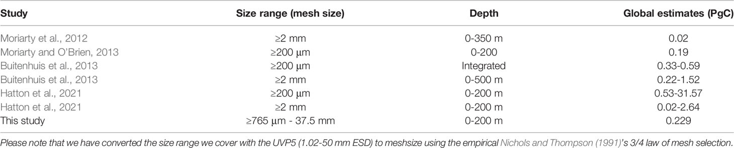
Table 2 Comparison of global biomass estimates in the literature.

4.5 Global Zooplankton Biomass Distribution

The distribution of the global integrated biomass (0-500 m) ad minima follows the patterns described by Ikeda (1985), Moriarty et al. (2012) and Hatton et al. (2021) which correspond to a latitudinal distribution of the biomass with high values north of 55°N and south of 55°S. Relatively higher values of biomass are predicted around the equator (15°N-15°S). The benefit of our work and of compiled datasets such as the ones used in Moriarty et al. (2012); Moriarty and O’Brien (2013), Buitenhuis et al. (2013) and Hatton et al. (2021) is that they bring together numerous single transects and allow to have an integrated view of global zooplankton distribution. The results depicted in Figure 11 in the Southern Ocean are consistent with a recent study done with BRTs (Pinkerton et al., 2020) showing that the highest environmental suitability for zooplankton was located between the Subantarctic Front and the southern limit of the Antarctic Circumpolar Current with a lower suitability north and south of this band. The spatial distribution of plankton biomass thus shows the importance of oceanographic hydrodynamics leading to oligotrophy in central gyres and mesotrophy in areas of high latitudes and equatorial and coastal upwellings. Zooplankton plays a crucial role in fisheries e.g. in the Humboldt Current System which harbors the largest fishery in the world and most economically important fish species, supported by the upwelling of Peru (Chavez et al., 2008). Peruvian anchovies and sardines obtain most of their energy from zooplankton (van der Lingen et al., 2009).

4.6 Conclusions and Outlook

In summary, our results show, for the first time, that spatial patterns and global biomass of key zooplankton groups can be calculated using a machine learning method (BRT) to extrapolate individual zooplankton biomass estimates from sparse UVP5 observation. They also highlight the important contribution of Rhizaria (predicted mainly in the intertropical range) and Copepoda (predicted mainly in high latitudes) to the global estimate of zooplankton biomass. Within the size range covered, Copepoda contributes 35.7%, Eumalacostraca 26.6% and Rhizaria 16.4% to global zooplankton biomass. This suggests that it is especially crucial to extend work on the fragile Rhizaria, which are comparatively little studied. As a biogeographical study, our aim was not to represent proximal mechanisms that drive the distribution of zooplankton, or to describe seasonal or transient (e.g. mesoscale) features, but rather to represent the global distribution patterns of biomass according to general properties of the water masses. This method worked well in general as seen in Figure 3 for at least 3 of the combinations of regions and depths. It made it possible to model 19 groups of zooplankton and obtain corresponding maps with the relative importance of the environmental variables used for the model. The WOA climatologies used in this study compile data of salinity and temperature (2005-2017) and other variables (1955-2017). The temporal coverage of the latter being much coarser, we hope to use more constrained nutrient datasets in our future work as they become available.

The zooplankton biomass predictions based on UVP5 datasets presented here are important for global biogeochemical modeling of pelagic ecosystems because they usually lack zooplankton observations to constrain their development (Stemmann and Boss, 2012; Buitenhuis et al., 2013; Séférian et al., 2020). A current trend is to add a more realistic representation of plankton in ecosystem models to better predict future ecosystem states and ocean conditions and to inform sustainable management strategies for climate mitigation at global scale (Séférian et al., 2020). The UVP5, the newly developed UVP6 (Picheral et al., 2021) and other commercialized in situ systems, provided that they are inter-calibrated (Lombard et al., 2019), will continue to be used in the foreseeable future, increasing data availability. Still, the bottleneck lies in the classification of the massive amount of images which still require human validation, but new algorithms to recognise plankton types and traits are expected (Irisson et al., 2022). The further anticipated expansion of image datasets will enable the quantitative assessment of rare groups that were not well predicted here. In addition, the deployment of the UVP6 on autonomous platforms will also help to sample certain areas that are difficult to access at certain times of the year such as polar regions in winter. The large dataset used in this study spans 10 years of data collection and can be compared to the COPEPOD database collected since about 1960. The possibilities given by imaging systems could hence help to reach a useful amount of data in a much smaller time frame. It would be interesting to use other imaging system’s data sets such as the ones presented by Lombard et al. (2019) to reconstruct the wider size spectrum of these groups in terms of biomass. To have a better understanding of the vertical habitat of zooplanktonic groups, we highly recommend that UVP5 and 6 profiles should be done to at least 1,000 m when the bathymetry allows it. Long term inter annual data acquisition is also highly recommended. This will enable us to monitor global zooplankton biomass changes at pace with the speed of global change.

Data Availability Statement

The inputs and outputs of the world models for 0-200 m and 200-500 m were uploaded to the GitHub repository: https://github.com/dlaetitia/Global_zooplankton_biomass_distribution.git. The code used for the models and the post treatment of their outputs was also made available in the same GitHub repository. The dataset of environmental data from World Ocean Atlas is available at https://www.ncei.noaa.gov/products/world-ocean-atlas. The surface chlorophyll a data is available on the Copernicus website at https://resources.marine.copernicus.eu/productdetail/OCEANCOLOUR_GLO_CHL_L4_REP_OBSERVATIONS_009_082/.

Author Contributions

LD, RK, LS, JO-I and TP developed the study’s concept; RK, LS, LD, FC, FL, MB, TB, LC, LG, HH, LK-B, AD, MP, AR, AW, contributed to data acquisition; RK, LS, LD, JO-I, TP contributed substantially to the data analysis; LD led the code development with major assistance by JO and guidance by TP and RK; LD created all figures and drafted the manuscript; All authors contributed substantially to drafting the manuscript; All authors approved the final submitted manuscript.

Funding

LD, RK and LS received support by the European Union project TRIATLAS (European Union Horizon 2020 program, grant agreement 817578) and the Sorbonne Université through the Ecole doctorale 129. LD was supported in the beginning of this project by the Laboratoire d'Océanographie de Villefranche-sur-mer (LOV). LS was supported in the initial phase of the development by the CNRS/Sorbonne University Chair VISION. RK furthermore acknowledges support via a Make Our Planet Great Again grant from the French National Research Agency (ANR) within the Programme d’Investissements d’Avenir (reference ANR-19-MPGA-0012). AR was funded by the PACES II (Polar Regions and Coasts in a Changing Earth System) program of the Helmholtz Association and the INSPIRES program of the Alfred Wegener Institute Helmholtz Centre for Polar and Marine Research. Some of the observations used in this study were funded by NASA grants #NNX15AE67G.

Conflict of Interest

The authors declare that the research was conducted in the absence of any commercial or financial relationships that could be construed as a potential conflict of interest.

The handling editor SP declared a shared affiliation with the author FL at the time of review.

Publisher’s Note

All claims expressed in this article are solely those of the authors and do not necessarily represent those of their affiliated organizations, or those of the publisher, the editors and the reviewers. Any product that may be evaluated in this article, or claim that may be made by its manufacturer, is not guaranteed or endorsed by the publisher.

Acknowledgments

The sampling effort on which this paper is based was enabled by the dedicated cruise leaders and participants who helped in the creation of the UVP5 dataset. We thank them as well as all the people who have participated in the classification of the huge amount of UVP5 images. We are grateful for the ship time provided by the respective institutions and programs. Furthermore, we would like to thank our colleagues from the Laboratoire d’Oceanographie de Villefranche (LOV) as well as Marina Levy and Fabio Benedetti for their support and precious guidance. We also thank Yawouvi Dodji Soviadan for his help with the Tara Oceans mission data.

Supplementary Material

The Supplementary Material for this article can be found online at: https://www.frontiersin.org/articles/10.3389/fmars.2022.894372/full#supplementary-material

References

Amante C., Eakins B. W. (2009). ETOPO1 1 Arc-Minute Global Relief Model: Procedures, Data Sources and Analysis. NOAA Technical Memorandum NESDIS NGDC-24. National Geophysical Data Center, NOAA. doi: 10.7289/V5C8276M [2021.01.19].
Antezana T. (2010). Euphausia Mucronata: A Keystone Herbivore and Prey of the Humboldt Current System. Deep. Sea. Res. Part II.: Top. Stud. Oceanogr. 57, 652–662. doi: 10.1016/j.dsr2.2009.10.014
Beaugrand G., Luczak C., Edwards M. (2009). Rapid Biogeographical Plankton Shifts in the North Atlantic Ocean. Global Change Biol. 15, 1790–1803. doi: 10.1111/j.1365-2486.2009.01848.x
Beers J. R., Stewart G. L. (1970). The Preservation of Acantharians in Fixed Plankton Samples. Limnol. Oceanogr. 15, 825–827. doi: 10.4319/lo.1970.15.5.0825
Bernstein R. E., Betzer P. R., Feely R. A., Byrne R. H., Lamb M. F., Michaels A. F. (1987). Acantharian Fluxes and Strontium to Chlorinity Ratios in the North Pacific Ocean. Science 237, 1490–1494. doi: 10.1126/science.237.4821.1490
Biard T., Ohman M. D. (2020). Vertical Niche Definition of Test-Bearing Protists (Rhizaria) Into the Twilight Zone Revealed by in Situ Imaging. Limnol. Oceanogr. 65, 2583–2602. doi: 10.1002/lno.11472
Biard T., Stemmann L., Picheral M., Mayot N., Vandromme P., Hauss H., et al. (2016). In Situ Imaging Reveals the Biomass of Giant Protists in the Global Ocean. Nature 532, 504–507. doi: 10.1038/nature17652
Boltovskoy D., Anderson O. R., Correa N. M. (2017). “Radiolaria and Phaeodaria,” in Handbook of the Protists. Eds. Archibald J. M., Simpson A. G., Slamovits C. H. (Cham: Springer International Publishing), 731–763. doi: 10.1007/978-3-319-28149-0_19
Bottazzi E. M., Andreoli M. G. (1982). Distribution of adult and juvenile Acantharia (Protozoa Sarcodina) in the Atlantic Ocean. Journal of Plankton Research, 4 (4), 757–777. doi: 10.1093/plankt/4.4.757
Breiman L., Friedman J. H., Olshen R. A., Stone C. J. (1984). Classification and Regression Trees (Wadsworth & Brooks. Cole Statistics/Probability Series).
Brinton E. (1967). Vertical Migration and Avoidance Capability of Euphausiids in the California Current. Limnol. Oceanogr. 12, 451–483. doi: 10.4319/lo.1967.12.3.0451._eprint:https://onlinelibrary.wiley.com/doi/pdf/10.4319/lo.1967.12.3.0451
Brodeur R., Perry I., Boldt J., Flostrand L., Galbraith M., King J., et al. (2018). An Unusual Gelatinous Plankton Event in the NE Pacific: The Great Pyrosome Bloom of 2017, Vol. 26. 6. Available at: https://www.researchgate.net/publication/322665037_An_unusual_gelatinous_plankton_event_in_the_NE_Pacific_The_Great_Pyrosome_Bloom_of_2017
Buesseler K. O., Boyd P. W. (2009). Shedding Light on Processes That Control Particle Export and Flux Attenuation in the Twilight Zone of the Open Ocean. Limnol. Oceanogr. 54, 1210–1232. doi: 10.4319/lo.2009.54.4.1210
Buitenhuis E. T., Vogt M., Moriarty R., Bednaršek N., Doney S. C., Leblanc K., et al. (2013). MAREDAT: Towards a World Atlas of MARine Ecosystem DATa. Earth Syst. Sci. Data 5, 227–239. doi: 10.5194/essd-5-227-2013
Castellanos I., Suárez-Morales E., Álvaro Morales-Ramírez Ã. (2009). “Euphausiids,” in Marine Biodiversity of Costa Rica, Central America, vol. 86. Eds. Wehrtmann I. S., Cortés J. (Dordrecht: Springer Netherlands), 199–207. doi: 10.1007/978-1-4020-8278-818
Chavez F. P., Bertrand A., Guevara-Carrasco R., Soler P., Csirke J. (2008). The Northern Humboldt Current System: Brief History, Present Status and a View Towards the Future. Prog. Oceanogr. 79, 95–105. doi: 10.1016/j.pocean.2008.10.012
Chen T., He T., Benesty M., Khotilovich V., Tang Y., Cho H., et al. (2021). Xgboost: Extreme Gradient Boosting.
Chen B., Liu H., Xiao W., Wang L., Huang B. (2020). A Machine-Learning Approach to Modeling Picophytoplankton Abundances in the South China Sea. Prog. Oceanogr. 189, 102456. doi: 10.1016/j.pocean.2020.102456
Christiansen S., Hoving H., Schütte F., Hauss H., Karstensen J., Körtzinger A., et al. (2018). Particulate Matter Flux Interception in Oceanic Mesoscale Eddies by the Polychaete Poeobius Sp. Limnol. Oceanogr. 63, 2093–2109. doi: 10.1002/lno.10926
Cowen R. K., Guigand C. M. (2008). In Situ Ichthyoplankton Imaging System (I SIIS): System Design and Preliminary Results: In Situ Ichthyoplankton Imaging System. Limnol. Oceanogr.: Methods 6, 126–132. doi: 10.4319/lom.2008.6.126
Culverhouse P. F. (2007). Human and Machine Factors in Algae Monitoring Performance. Ecol. Inf. 2, 361–366. doi: 10.1016/j.ecoinf.2007.07.001
Culverhouse P. F., Macleod N., Williams R., Benfield M. C., Lopes R. M., Picheral M. (2014). An Empirical Assessment of the Consistency of Taxonomic Identifications. Mar. Biol. Res. 10, 73–84. doi: 10.1080/17451000.2013.810762
Dai L., Li C., Yang G., Sun X. (2016). Zooplankton Abundance, Biovolume and Size Spectra at Western Boundary Currents in the Subtropical North Pacific During Winter 2012. J. Mar. Syst. 155, 73–83. doi: 10.1016/j.jmarsys.2015.11.004
Davis C. S., Gallager S. M., Solow A. R. (1992). Microaggregations of Oceanic Plankton Observed by Towed Video Microscopy. Science 257, 230–232. doi: 10.1126/science.257.5067.230
Davis C. S., Thwaites F. T., Gallager S. M., Hu Q. (2005). A Three-Axis Fast-Tow Digital Video Plankton Recorder for Rapid Surveys of Plankton Taxa and Hydrography: New Video Plankton Recorder. Limnol. Oceanogr.: Methods 3, 59–74. doi: 10.4319/lom.2005.3.59
De’ath G. (2007). Boosted Trees for Ecological Modeling and Prediction. Ecology 88, 243–251. doi: 10.1890/0012-9658(2007)88[243:BTFEMA]2.0.CO;2
Decelle J., Martin P., Paborstava K., Pond D. W., Tarling G., Mahé F., et al. (2013). Diversity, Ecology and Biogeochemistry of Cyst-Forming Acantharia (Radiolaria) in the Oceans. PLoS One 8, e53598. doi: 10.1371/journal.pone.0053598
Decelle J., Not F. (2015). “Acantharia,” in eLS, 1 edn (John Wiley & Sons, Ltd (Wiley), 1–10. doi: 10.1002/9780470015902.a0002102.pub2
de Vargas C., Audic S., Henry N., Decelle J., Mahe F., Logares R., et al. (2015). Eukaryotic plankton diversity in the sunlit ocean. Science 348, 1261605.5 –126160511. doi: 10.1126/science.1261605
Edwards M., Hélaouët P., Goberville E., Lindley A., Tarling G. A., Burrows M. T., et al. (2021). North Atlantic Warming Over Six Decades Drives Decreases in Krill Abundance With No Associated Range Shift. Commun. Biol. 4, 644. doi: 10.1038/s42003-021-02159-1
Elith J., Graham C. H. (2009). Do They? How do They? WHY do They Differ? On Finding Reasons for Differing Performances of Species Distribution Models. Ecography 32, 66–77. doi: 10.1111/j.1600-0587.2008.05505.x
Elith J., Graham C. H., Anderson R. P., Dudík M., Ferrier S., Guisan A., et al. (2006). Novel Methods Improve Prediction of Species’ Distributions From Occurrence Data. Ecography 29, 129–151. doi: 10.1111/j.2006.0906-7590.04596.x
Elith J., Leathwick J. R. (2009). Species Distribution Models: Ecological Explanation and Prediction Across Space and Time. Annu. Rev. Ecol. Evol. Syst. 40, 677–697. doi: 10.1146/annurev.ecolsys.110308.120159
Elith J., Leathwick J. R., Hastie T. (2008). A Working Guide to Boosted Regression Trees. J. Anim. Ecol. 77, 802–813. doi: 10.1111/j.1365-2656.2008.01390.x
Faillettaz R., Picheral M., Luo J. Y., Guigand C., Cowen R. K., Irisson J.-O. (2016). Imperfect Automatic Image Classification Successfully Describes Plankton Distribution Patterns. Methods Oceanogr. 15-16, 60–77. doi: 10.1016/j.mio.2016.04.003
Forest A., Stemmann L., Picheral M., Burdorf L., Robert D., Fortier L., et al. (2012). Size Distribution of Particles and Zooplankton Across the Shelf-Basin System in Southeast Beaufort Sea: Combined Results From an Underwater Vision Profiler and Vertical Net Tows. Biogeosciences 9, 1301–1320. doi: 10.5194/bg-9-1301-2012
Friedman J. H. (2002). Stochastic Gradient Boosting. Comput. Stat Data Anal. 38, 367–378. doi: 10.1016/S0167-9473(01)00065-2
Gallienne C. P. (2001). Is Oithona the Most Important Copepod in the World’s Oceans? J. Plankt. Res. 23, 1421–1432. doi: 10.1093/plankt/23.12.1421
Garcia H. E., Boyer T.P., Baranova O. K., Locarnini R. A., Mishonov A.V., Grodsky A., et al (2019). World Ocean Atlas 2018: Product Documentation. A. Mishonov, Technical Editor.
González Carman V., Piola A., O’Brien T. D., Tormosov D. D., Acha E. M. (2019). Circumpolar Frontal Systems as Potential Feeding Grounds of Southern Right Whales. Prog. Oceanogr. 176, 102123. doi: 10.1016/j.pocean.2019.102123
Gorsky G., Ohman M. D., Picheral M., Gasparini S., Stemmann L., Romagnan J.-B., et al. (2010). Digital Zooplankton Image Analysis Using the ZooScan Integrated System. J. Plankt. Res. 32, 285–303. doi: 10.1093/plankt/fbp124
Griffith A. W., Gobler C. J. (2020). Harmful Algal Blooms: A Climate Change Co-Stressor in Marine and Freshwater Ecosystems. Harmf. Algae. 91, 101590. doi: 10.1016/j.hal.2019.03.008
Grossmann M. M., Gallager S. M., Mitarai S. (2015). Continuous Monitoring of Near-Bottom Mesoplankton Communities in the East China Sea During a Series of Typhoons. J. Oceanogr. 71, 115–124. doi: 10.1007/s10872-014-0268-y
Guidi L., Stemmann L., Jackson G. A., Ibanez F., Claustre H., Legendre L., et al. (2009). Effects of Phytoplankton Community on Production, Size, and Export of Large Aggregates: A World-Ocean Analysis. Limnol. Oceanogr. 54, 1951–1963. doi: 10.4319/lo.2009.54.6.1951
Guihen D., Brearley J. A., Fielding S. (2022). Antarctic Krill Likely Avoid Underwater Gliders. Deep. Sea. Res. Part I.: Oceanogr. Res. Pap. 179, 103680. doi: 10.1016/j.dsr.2021.103680
Guisan A., Zimmermann N. E. (2000). Predictive Habitat Distribution Models in Ecology. Ecol. Model. 135, 147–186. doi: 10.1016/S0304-3800(00)00354-9
Hastie T., Tibshirani R., Friedman J. (2001). The Elements of Statistical Learning. 2nd ed. (Springer).
Hatton I. A., Heneghan R. F., Bar-On Y. M., Galbraith E. D. (2021). The Global Ocean Size-Spectrum From Bacteria to Whales. Preprint, Ecology. doi: 10.1101/2021.04.03.438320
Hays G., Richardson A., Robinson C. (2005). Climate Change and Marine Plankton. Trends Ecol. Evol. 20, 337–344. doi: 10.1016/j.tree.2005.03.004
Hoving H.-J., Christiansen S., Fabrizius E., Hauss H., Kiko R., Linke P., et al. (2019). The Pelagic In Situ Observation System (PELAGIOS) to Reveal Biodiversity, Behavior, and Ecology of Elusive Oceanic Fauna. Ocean. Sci. 15, 1327–1340. doi: 10.5194/os-15-1327-2019
Hu C., Xu J., Li X., Shi Z., Li R. (2021). Environmental Regulations on Bacterial Abundance in the South China Sea Inferred From Regression Models. Sci. Tot. Environ. 774, 146315. doi: 10.1016/j.scitotenv.2021.146315
Hwang J.-S., Kumar R., Dahms H.-U., Tseng L.-C., Chen Q.-C. (2007). Mesh Size Affects Abundance Estimates of Oithona Spp. (Copepoda, Cyclopoida). Crustaceana 80, 827–837. doi: 10.1163/156854007781363169
Ibarbalz F. M., Henry N., Brandão M. C., Martini S., Busseni G., Byrne H., et al. (2019). Global Trends in Marine Plankton Diversity Across Kingdoms of Life. Cell 179, 1084–1097. doi: 10.1016/j.cell.2019.10.008
Ikeda T. (1985). Metabolic Rates of Epipelagic Marine Zooplankton as a Function of Body Mass and Temperature. Mar. Biol. 85, 1–11. doi: 10.1007/BF00396409
Ikenoue T., Kimoto K., Okazaki Y., Sato M., Honda M. C., Takahashi K., et al. (2019). Phaeodaria: An Important Carrier of Particulate Organic Carbon in the Mesopelagic Twilight Zone of the North Pacific Ocean. Global Biogeochem. Cycle. 33, 1146–1160. doi: 10.1029/2019GB006258
Irisson J.-O., Ayata S.-D., Lindsay D. J., Karp-Boss L., Stemmann L. (2022). Machine Learning for the Study of Plankton and Marine Snow From Images. Annu. Rev. Mar. Sci. 14, annurev–marine–041921–013023. doi: 10.1146/annurev-marine-041921-013023
Karsenti E., Acinas S. G., Bork P., Bowler C., De Vargas C., Raes J., et al. (2011). A Holistic Approach to Marine Eco-Systems Biology. PLoS Biology 9, e1001177.1–5. doi: 10.1371/journal.pbio.1001177
Kiørboe T. (2013). Zooplankton Body Composition. Limnol. Oceanogr. 58, 1843–1850. doi: 10.4319/lo.2013.58.5.1843
Lampitt R. S., Salter I., Johns D. (2009). Radiolaria: Major Exporters of Organic Carbon to the Deep Ocean. Global Biogeochem. Cycle. 23. doi: 10.1029/2008GB003221
Leathwick J., Elith J., Francis M., Hastie T., Taylor P. (2006). Variation in Demersal Fish Species Richness in the Oceans Surrounding New Zealand: An Analysis Using Boosted Regression Trees. Mar. Ecol. Prog. Ser. 321, 267–281. doi: 10.3354/meps321267
Lehodey P., Alheit J., Barange M., Baumgartner T., Beaugrand G., Drinkwater K., et al. (2006). Climate Variability, Fish, and Fisheries. J. Climate 19, 5009–5030. doi: 10.1175/JCLI3898.1
Le Quéré C., Buitenhuis E. T., Moriarty R., Alvain S., Aumont O., Bopp L., et al. (2016). Role of Zooplankton Dynamics for Southern Ocean Phytoplankton Biomass Andglobal Biogeochemical Cycles. Biogeosciences 13, 4111–4133. doi: 10.5194/bg-13-4111-2016
Lombard F., Boss E., Waite A. M., Vogt M., Uitz J., Stemmann L., et al. (2019). EnglishGlobally Consistent Quantitative Observations of Planktonic Ecosystems. Front. Mar. Sci. 6. doi: 10.3389/fmars.2019.00196
Lombard F., Kiørboe T. (2010). Marine Snow Originating From Appendicularian Houses: Age-Dependent Settling Characteristics. Deep. Sea. Res. Part I.: Oceanogr. Res. Pap. 57, 1304–1313. doi: 10.1016/j.dsr.2010.06.008
Lombard F., Renaud F., Sainsbury C., Sciandra A., Gorsky G. (2009). Appendicularian Ecophysiology I. J. Mar. Syst. 78, 606–616. doi: 10.1016/j.jmarsys.2009.01.004
Longhurst A. (1995). Seasonal Cycles of Pelagic Production and Consumption. Prog. Oceanogr. 36, 77–167. doi: 10.1016/0079-6611(95)00015-1
Longhurst A. R., Glen Harrison W. (1989). The Biological Pump: Profiles of Plankton Production and Consumption in the Upper Ocean. Prog. Oceanogr. 22, 47–123. doi: 10.1016/0079-6611(89)90010-4
Lucas C. H., Jones D. O. B., Hollyhead C. J., Condon R. H., Duarte C. M., Graham W. M., et al. (2014). Gelatinous Zooplankton Biomass in the Global Oceans: Geographic Variation and Environmental Drivers: Global Gelatinous Biomass. Global Ecol. Biogeogr. 23, 701–714. doi: 10.1111/geb.12169
Mansour J. S., Norlin A., Llopis Monferrer N., L’Helguen S., Not F. (2021). Carbon and Nitrogen Content to Biovolume Relationships for Marine Protist of the Rhizaria Lineage (Radiolaria and Phaeodaria). Limnol. Oceanogr. 66, 1703–1717. doi: 10.1002/lno.11714
McConville K., Atkinson A., Fileman E. S., Spicer J. I., Hirst A. G. (2016). Disentangling the Counteracting Effects of Water Content and Carbon Mass on Zooplankton Growth. J. Plankt. Res. 39 (2), 246–256. doi: 10.1093/plankt/fbw094
McGinty N., Barton A. D., Record N. R., Finkel Z. V., Johns D. G., Stock C. A., et al. (2021). Anthropogenic Climate Change Impacts on Copepod Trait Biogeography. Global Change Biol. 27, 1431–1442. doi: 10.1111/gcb.15499
Michaels A. F. (1988). Vertical Distribution and Abundance of Acantharia and Their Symbionts. Mar. Biol. 97, 559–569. doi: 10.1007/BF00391052
Michaels A. F. (1991). Acantharian Abundance and Symbiont Productivity at the VERTEX Seasonal Station. J. Plankt. Res. 13, 399–418. doi: 10.1093/plankt/13.2.399
Moriarty R., Buitenhuis E. T., Le Quéré C., Gosselin M.-P. (2012). Distribution of Known Macrozooplankton Abundance and Biomass in the Global Ocean. Earth Syst. Sci. Data Discuss. 5, 187–220. doi: 10.5194/essdd-5-187-2012
Moriarty R., O’Brien T. D. (2013). Distribution of Mesozooplankton Biomass in the Global Ocean. Earth Syst. Sci. Data 5, 45–55. doi: 10.5194/essd-5-45-2013
Morley J., Stepien J. (1984). Siliceous Microfauna in Waters Beneath Antarctic Sea Ice. Mar. Ecol. Prog. Ser. 19, 207–210. doi: 10.3354/meps019207
Nakamura Y., Imai I., Yamaguchi A., Tuji A., Suzuki N. (2013). Aulographis Japonica Sp. Nov. (Phaeodaria, Aulacanthida, Aulacanthidae), an Abundant Zooplankton in the Deep Sea of the Sea of Japan. Plankt. Bentho. Res. 8, 107–115. doi: 10.3800/pbr.8.107
Nakamura Y., Suzuki N. (2015). “Phaeodaria: Diverse Marine Cercozoans of World-Wide Distribution,” in Marine Protists. Eds. Ohtsuka S., Suzaki T., Horiguchi T., Suzuki N., Not F. (Tokyo: Springer Japan), 223–249. doi: 10.1007/978-4-431-55130-0_9
Nelder J. A., Wedderburn R. W. M. (1972). Journal of the Royal Statistical Society. Series A (General) 135(3):370–384 (15 pages) doi: 10.2307/2344614
Nichols J., Thompson A. (1991). Mesh Selection of Copepodite and Nauplius Stages of Four Calanoid Copepod Species. J. Plankt. Res. 13, 661–671. doi: 10.1093/plankt/13.3.661
Ohman M. D. (2019). A Sea of Tentacles: Optically Discernible Traits Resolved From Planktonic Organisms in Situ. ICES. J. Mar. Sci. 76, 1959–1972. doi: 10.1093/icesjms/fsz184
Pesant S., Not F., Picheral M., Kandels-Lewis S., Le Bescot N., Gorsky G., et al. (2015). Open Science Resources for the Discovery and Analysis of Tara Oceans Data. Sci. Data 2, 150023. doi: 10.1038/sdata.2015.23
Pettitt-Wade H., Pearce T., Kuptana D., Gallagher C. P., Scharffenberg K., Lea E. V., et al. (2020). Inuit Observations of a Tunicata Bloom Unusual for the Amundsen Gulf, Western Canadian Arctic. Arct. Sci. 6, 340–351. doi: 10.1139/as-2020-0018
Phillips S. J., Anderson R. P., Schapire R. E. (2006). Maximum Entropy Modeling of Species Geographic Distributions. Ecol. Model. 190, 231–259. doi: 10.1016/j.ecolmodel.2005.03.026
Picheral M., Catalano C., Brousseau D., Claustre H., Coppola L., Leymarie E., et al. (2021). The Underwater Vision Profiler 6: An Imaging Sensor of Particle Size Spectra and Plankton, for Autonomous and Cabled Platforms. Limnol. Oceanogr.: Methods 20, 115–129. doi: 10.1002/lom3.10475. lom3.10475.
Picheral M., Colin S., Irisson J.-O. (2017). EcoTaxa, a Tool for the Taxonomic Classification of Images.
Picheral M., Guidi L., Stemmann L., Karl D. M., Iddaoud G., Gorsky G. (2010). The Underwater Vision Profiler 5: An Advanced Instrument for High Spatial Resolution Studies of Particle Size Spectra and Zooplankton: Underwater Vision Profiler. Limnol. Oceanogr.: Methods 8, 462–473. doi: 10.4319/lom.2010.8.462
Pinkerton M. H., Décima M., Kitchener J. A., Takahashi K. T., Robinson K. V., Stewart R., et al. (2020). Zooplankton in the Southern Ocean From the Continuous Plankton Recorder: Distributions and Long-Term Change. Deep. Sea. Res. Part I.: Oceanogr. Res. Pap. 162, 103303. doi: 10.1016/j.dsr.2020.103303
R Core Team (2021). R: A Language and Environment for Statistical Computing (Vienna, Austria: R Foundation for Statistical Computing).
Remsen A., Hopkins T. L., Samson S. (2004). What You See is Not What You Catch: A Comparison of Concurrently Collected Net, Optical Plankton Counter, and Shadowed Image Particle Profiling Evaluation Recorder Data From the Northeast Gulf of Mexico. Deep. Sea. Res. Part I.: Oceanogr. Res. Pap. 51, 129–151. doi: 10.1016/j.dsr.2003.09.008
Richardson A. J., Bakun A., Hays G. C., Gibbons M. J. (2009). The Jellyfish Joyride: Causes, Consequences and Management Responses to a More Gelatinous Future. Trends Ecol. Evol. 24, 312–322. doi: 10.1016/j.tree.2009.01.010
Rombouts I., Beaugrand G., Ibaňez F., Gasparini S., Chiba S., Legendre L. (2009). Global Latitudinal Variations in Marine Copepod Diversity and Environmental Factors. Proc. R. Soc. B.: Biol. Sci. 276, 3053–3062. doi: 10.1098/rspb.2009.0742
Sameoto D., Cochrane N., Herman A. (1993). Convergence of Acoustic, Optical, and Net-Catch Estimates of Euphausiid Abundance: Use of Artificial Light to Reduce Net. Can. J. Fish. Aquat. Sci. 50, 334–346. doi: 10.1139/f93-039
Schapire R. E. (2003). “The Boosting Approach to Machine Learning: An Overview,” in Nonlinear Estimation and Classification. Eds. Denison D. D., Hansen M. H., Holmes C. C., Mallick B., Yu B. (New York, NY: Springer), 149–171. Lecture Notes in Statistics. doi: 10.1007/978-0-387-21579-2_9
Schulz J., Barz K., Ayon P., Ludtke A., Zielinski O., Mengedoht D., et al. (2010). Imaging of Plankton Specimens With the Lightframe on-Sight Keyspecies Investigation (LOKI) System. J. Eur. Optic. Soc.: Rapid Publicat. 5, 10017s. doi: 10.2971/jeos.2010.10017s
Séférian R., Berthet S., Yool A., Palmieri J., Bopp L., Tagliabue A., et al. (2020). Tracking Improvement in Simulated Marine Biogeochemistry Between CMIP5 and CMIP6. Curr. Climate Change Rep. 6, 95–119. doi: 10.1007/s40641-020-00160-0
Siegel V. (2005). Distribution and Population Dynamics of Euphausia Superba: Summary of Recent Findings. Pol. Biol. 29, 1–22. doi: 10.1007/s00300-005-0058-5
Siegel V. (Ed.) (2016). “Biology and Ecology of Antarctic Krill,” in Advances in Polar Ecology (Cham: Springer International Publishing). doi: 10.1007/978-3-319-29279-3
Son D., Cho H., Lee E. J. (2018). Determining Factors for the Occurrence and Richness of Submerged Macrophytes in Major Korean Rivers. Aquat. Bot. 150, 82–88. doi: 10.1016/j.aquabot.2018.07.003
Soviadan Y. D., Benedetti F., Brandão M. C., Ayata S.-D., Irisson J.-O., Jamet J. L., et al. (2022). Patterns of Mesozooplankton Community Composition and Vertical Fluxes in the Global Ocean. Prog. Oceanogr. 200, 102717. doi: 10.1016/j.pocean.2021.102717
Steinberg D. K., Cope J. S., Wilson S. E., Kobari T. (2008). A Comparison of Mesopelagic Mesozooplankton Community Structure in the Subtropical and Subarctic North Pacific Ocean. Deep. Sea. Res. Part II.: Top. Stud. Oceanogr. 55, 1615–1635. doi: 10.1016/j.dsr2.2008.04.025
Steinberg D. K., Landry M. R. (2017). Zooplankton and the Ocean Carbon Cycle. Annu. Rev. Mar. Sci. 9, 413–444. doi: 10.1146/annurev-marine-010814-015924
Stemmann L., Boss E. (2012). Plankton and Particle Size and Packaging: From Determining Optical Properties to Driving the Biological Pump. Annu. Rev. Mar. Sci. 4, 263–290. doi: 10.1146/annurev-marine-120710-100853
Stemmann L., Gorsky G., Marty J.-C., Picheral M., Miquel J.-C. (2002). Four-Year Study of Large-Particle Vertical Distribution (0–1000 M) in the NW Mediterranean in Relation to Hydrology, Phytoplankton, and Vertical Flux. Deep. Sea. Res. Part II.: Top. Stud. Oceanogr. 49, 2143–2162. doi: 10.1016/S0967-0645(02)00032-2
Stemmann L., Youngbluth M., Robert K., Hosia A., Picheral M., Paterson H., et al. (2008). Global Zoogeography of Fragile Macrozooplankton in the Upper 100–1000 M Inferred From the Underwater Video Profiler. ICES. J. Mar. Sci. 65, 433–442. doi: 10.1093/icesjms/fsn010
Stukel M. R., Biard T., Krause J., Ohman M. D. (2018). Large Phaeodaria in the Twilight Zone: Their Role in the Carbon Cycle: Phaeodarian Ecology in the Twilight Zone. Limnol. Oceanogr. 63, 2579–2594. doi: 10.1002/lno.10961
Stukel M. R., Ohman M. D., Kelly T. B., Biard T. (2019). The Roles of Suspension-Feeding and Flux-Feeding Zooplankton as Gatekeepers of Particle Flux Into the Mesopelagic Ocean in the Northeast Pacific. Front. Mar. Sci. 6. doi: 10.3389/fmars.2019.00397
Sun H., Benzie P., Burns N., Hendry D., Player M., Watson J. (2008). Underwater Digital Holography for Studies of Marine Plankton. Philos. Trans. R. Soc. A.: Math. Phys. Eng. Sci. 366, 1789–1806. doi: 10.1098/rsta.2007.2187
Sunday J. M., Bates A. E., Dulvy N. K. (2012). Thermal Tolerance and the Global Redistribution of Animals. Nat. Climate Change 2, 686–690. doi: 10.1038/nclimate1539
Suthers I., Rissik D., Richardson A. (2019). Plankton: A Guide to Their Ecology and Monitoring for Water Quality (Csiro Publishing). Google-Books-ID: e8uPDwAAQBAJ). Available at: https://www.researchgate.net/publication/265624443_Plankton_A_Guide_to_Their_Ecology_and_Monitoring_for_Water_Quality
Suzuki N., Not F. (2015). “Biology and Ecology of Radiolaria,” in Marine Protists. Eds. Ohtsuka S., Suzaki T., Horiguchi T., Suzuki N., Not F. (Tokyo: Springer Japan), 179–222. doi: 10.1007/978-4-431-55130-0_8
Turner J. T. (2002). Zooplankton Fecal Pellets, Marine Snow and Sinking Phytoplankton Blooms. Aquat. Microbial. Ecol. 27, 57–102. doi: 10.3354/ame027057
Turner J. T. (2004). The Importance of Small Planktonic Copepods and Their Roles in Pelagic Marine Food Webs. Zool. Stud. 43, 255–266.
Turner J. T. (2015). Zooplankton Fecal Pellets, Marine Snow, Phytodetritus and the Ocean’s Biological Pump. Prog. Oceanogr. 130, 205–248. doi: 10.1016/j.pocean.2014.08.005
van der Lingen C., Bertrand A., Bode A., Brodeur R., Cubillos L., Espinoza P., et al. (2009). Trophic Dynamics of Small Pelagic Fish 333–403.
van der Lingen C., Hutchings L., Field J. (2006). Comparative Trophodynamics of Anchovy Engraulis Encrasicolus and Sardine Sardinops Sagax in the Southern Benguela: Are Species Alternations Between Small Pelagic Fish Trophodynamically Mediated? Afr. J. Mar. Sci. 28, 465–477. doi: 10.2989/18142320609504199
Wiebe P. H., Boyd S. H., Davis M., Cox J. L. (1982). Avoidance of Towed Nets by the Euphausiid Nematoscelis Megalops. Fish. Bull. 80, 75–91. doi: 10.1080/03610918.2020.1772302
Wiebe P. H., Morton A. W., Bradley A. M., Backus R. H., Craddock J. E., Barber V., et al. (1985). New Development in the MOCNESS, an Apparatus for Sampling Zooplankton and Micronekton. Mar. Biol. 87, 313–323. doi: 10.1007/BF00397811
Zhang M., Straile D., Chen F., Shi X., Yang Z., Cai Y., et al. (2018). Dynamics and Drivers of Phytoplankton Richness and Composition Along Productivity Gradient. Sci. Tot. Environ. 625, 275–284. doi: 10.1016/j.scitotenv.2017.12.288
Keywords: global zooplankton, in situ imaging, biomass, machine learning, underwater vision profiler (UVP), spatial distribution, boosted regression trees (BRT), habitat modeling
Citation: Drago L, Panaïotis T, Irisson J-O, Babin M, Biard T, Carlotti F, Coppola L, Guidi L, Hauss H, Karp-Boss L, Lombard F, McDonnell AMP, Picheral M, Rogge A, Waite AM, Stemmann L and Kiko R (2022) Global Distribution of Zooplankton Biomass Estimated by In Situ Imaging and Machine Learning. Front. Mar. Sci. 9:894372. doi: 10.3389/fmars.2022.894372
Received: 11 March 2022; Accepted: 05 May 2022;
Published: 09 August 2022.
Edited by:
Sophie G. Pitois, Fisheries and Aquaculture Science (CEFAS), United KingdomCopyright © 2022 Drago, Panaïotis, Irisson, Babin, Biard, Carlotti, Coppola, Guidi, Hauss, Karp-Boss, Lombard, McDonnell, Picheral, Rogge, Waite, Stemmann and Kiko. This is an open-access article distributed under the terms of the Creative Commons Attribution License (CC BY). The use, distribution or reproduction in other forums is permitted, provided the original author(s) and the copyright owner(s) are credited and that the original publication in this journal is cited, in accordance with accepted academic practice. No use, distribution or reproduction is permitted which does not comply with these terms.
*Correspondence: Laetitia Drago, laetitia.drago@imev-mer.fr; Lars Stemmann, lars.stemmann@imev-mer.fr; Rainer Kiko, rainer.kiko@imev-mer.fr
†These authors share last authorship