Uncertainties in the Projected Patterns of Wave-Driven Longshore Sediment Transport Along a Non-straight Coastline
 Amin Reza Zarifsanayei1,2
  José A. A. Antolínez3*
  Amir Etemad-Shahidi1,2,4 Nick Cartwright1,2
  Darrell Strauss1,2 Gil Lemos5
- 1School of Engineering and Built Environment, Griffith University, Gold Coast, QLD, Australia
- 2Coastal and Marine Research Centre (CMRC), Griffith University, Gold Coast, QLD, Australia
- 3Department of Hydraulic Engineering, Faculty of Civil Engineering and Geosciences, Delft University of Technology, Delft, Netherlands
- 4School of Engineering, Edith Cowan University, Perth, WA, Australia
- 5Instituto Dom Luiz (IDL), Faculdade de Ciências, Universidade de Lisboa, Lisboa, Portugal
This study quantifies the uncertainties in the projected changes in potential longshore sediment transport (LST) rates along a non-straight coastline. Four main sources of uncertainty, including the choice of emission scenarios, Global Circulation Model-driven offshore wave datasets (GCM-Ws), LST models, and their non-linear interactions were addressed through two ensemble modelling frameworks. The first ensemble consisted of the offshore wave forcing conditions without any bias correction (i.e., wave parameters extracted from eight datasets of GCM-Ws for baseline period 1979–2005, and future period 2081–2100 under two emission scenarios), a hybrid wave transformation method, and eight LST models (i.e., four bulk formulae, four process-based models). The differentiating factor of the second ensemble was the application of bias correction to the GCM-Ws, using a hindcast dataset as the reference. All ensemble members were weighted according to their performance to reproduce the reference LST patterns for the baseline period. Additionally, the total uncertainty of the LST projections was decomposed into the main sources and their interactions using the ANOVA method. Finally, the robustness of the LST projections was checked. Comparison of the projected changes in LST rates obtained from two ensembles indicated that the bias correction could relatively reduce the ranges of the uncertainty in the LST projections. On the annual scale, the contribution of emission scenarios, GCM-Ws, LST models and non-linear interactions to the total uncertainty was about 10–20, 35–50, 5–15, and 30–35%, respectively. Overall, the weighted means of the ensembles reported a decrease in net annual mean LST rates (less than 10% under RCP 4.5, a 10–20% under RCP 8.5). However, no robust projected changes in LST rates on annual and seasonal scales were found, questioning any ultimate decision being made using the means of the projected changes.
Introduction
Coastal areas are of major importance for the development of cities and infrastructure as they provide economic benefits to their communities. The global distribution of the human population confirms that the world’s coastlines are more densely populated than other land regions (Jones et al., 2016). Sandy coasts can act as natural barriers to protect coastal regions from inundation by storm surge and wave action (e.g., Hanley et al., 2014), while also supporting important ecosystems. However, due to growing threats posed by natural and human-induced climate change, coastal systems are among the most endangered systems worldwide (Martinez and Psuty, 2004).
Along open sandy coasts, wave energy is one of the main drivers of coastal sediment transport. The gradient in longshore sediment transport (LST) is one of the key processes shaping sandy coasts on decadal timescales (Splinter and Coco, 2021). Hence, any changes in wave forcing might lead to remarkable changes in patterns of LST and long-term coastal evolution (e.g., Adams et al., 2011; Anderson et al., 2018; Başaran and Arı Güner, 2021; Vitousek et al., 2021). In recent years, several studies have shown that the offshore wind and wave patterns around the world are projected to be impacted by global and regional climate change (hereafter CC) by the end of this century (e.g., Hemer and Trenham, 2016; Camus et al., 2017; Lemos et al., 2019, 2021a,b; Morim et al., 2020). These changes are also visible in nearshore zones, modifying the patterns of erosion and accretion. Wave CC-induced coastal evolution can also be comparable to sea level rise-driven erosion (e.g., Vitousek et al., 2017).
Estimation of global warming impacts on wave climate is a very challenging task as it requires first projecting future climate variables and then simulating future offshore wave characteristics. Earth climate systems are simulated using sophisticated models, known as Global Circulation Models (GCMs). Although these models are valuable tools to investigate past, present, and future projected climates, they might offer highly uncertain projections (IPCC, 2014). The GCMs main outputs (i.e., near-surface wind speeds, sea level pressure and sea-ice coverage) are used to force wave models on a global scale and produce wave climate simulations or future projections (hereafter GCM-driven waves/GCM-Ws; e.g., Hemer and Trenham, 2016; Camus et al., 2017).
As the simulated offshore waves have significant biases, compared to reanalyses hindcast datasets of waves (e.g., Hersbach et al., 2020; Smith et al., 2020), there have been some efforts to correct the biases in the projected offshore waves for a baseline period, and then to apply the correction factors to future-period data (e.g., Lemos et al., 2020a,b). Nevertheless, the influence of such efforts on manipulating (i.e., amplifying/decreasing) the original signals of CC (the ones presented by GCM-Ws without bias correction) needs more investigation (Maraun, 2016). Future nearshore waves are projected by using the offshore GCM-Ws downscaled to nearshore areas through different wave transformation approaches (e.g., Antolínez et al., 2018). Finally, to project future sediment transport patterns, the projected nearshore waves need to be introduced to sediment transport models. Since the sediment transport models calibrated under specific forcing conditions (e.g., historical forcing) can respond differently to the new ones (e.g., future forcing conditions), using more than one sediment transport model (i.e., an ensemble of sediment transport models) is suggested for the CC assessment studies dealing with uncertainty issues (e.g., Zarifsanayei et al., 2020, 2022). Coastal management plans require quantitative and qualitative estimates of future sediment transport and coastal evolution. On the other hand, any projection requires dealing with various sources of uncertainties cascading through the aforementioned modelling processes (Ranasinghe, 2016; Toimil et al., 2020).
In the last decade, there have been some efforts to consider the importance of uncertainty evolution for the estimates of CC impacts on LST patterns. For instance, Adams et al. (2011) adopted a rough method to explore the possible impacts of CC on LST while addressing only offshore wave forcing uncertainty. The method was similar to Ruggiero et al. (2010), in which the offshore wave forcing (usually offshore wave direction) was manipulated to mimic the impacts of CC. Recently, the uncertainty of offshore forcing conditions has been addressed in a more complicated manner, using the outputs of GCMs, projected under different emission scenarios (e.g., Hemer and Trenham, 2016; Camus et al., 2017). Nevertheless, mainly due to the large computational costs of wave transformation through the state-of-art spectral wave models, usually only a limited number of GCMs (an ensemble of them) under one or two emission scenarios were considered for coastal sediment transport studies (e.g., Bonaldo et al., 2015; Dastgheib et al., 2016). In some cases, to decrease the computational costs of the studies, projected offshore waves were transferred to the nearshore zone through a simplified wave transformation method (e.g., Zacharioudaki and Reeve, 2011; Almar et al., 2015; Casas-Prat et al., 2016; Chowdhury et al., 2020). However, it is possible to significantly decrease the computational costs of spectral wave transformation by using hybrid methods (i.e., a combination of spectral models and machine learning techniques), retaining the required accuracy for sediment transport studies (e.g., Camus et al., 2011; Antolínez et al., 2016; Cagigal et al., 2020). Commonly, to project future LST patterns, the transformed waves (i.e., projected nearshore waves) are introduced to bulk transport formulae (e.g., Casas-Prat et al., 2016; Dastgheib et al., 2016; Chowdhury et al., 2020; Alvarez-Cuesta et al., 2021). In this way, the computational costs of sediment transport simulations are decreased. A few studies have tried to employ a more complex sediment transport model (i.e., process-based model; e.g., Bonaldo et al., 2015; O’Grady et al., 2019). To the knowledge of the authors, sampling and quantifying uncertainties from the common sources of uncertainty (namely of emission scenarios, GCM-Ws, LST models, and their non-linear interactions) in a systematic way, has been overlooked in the literature. As a result, the level of confidence of the projections has not been clearly reported. Moreover, applying the bias correction methods to the projected forcing conditions and its influence on narrowing or widening uncertainties in the projection of future sediment transport patterns (e.g., Toimil et al., 2021), has not yet been well examined.
This manuscript aims to employ an ensemble modelling framework to quantify the uncertainty in the projections of LST rates using the Gold Coast in southeast Queensland, Australia, as a study site. The framework consists of two emission scenarios (i.e., RCP 4.5, RCP 8.5), eight GCM-Ws (i.e., projected offshore wave datasets of CSIRO), a hybrid wave transformation method to reconstruct the whole time series of nearshore waves, and eight LST models (i.e., bulk formulae and process-based models). The framework is individually forced with both original and bias-corrected wave datasets to investigate the uncertainty of LST projections offered by each forcing dataset. Moreover, a variance-based approach is employed to find the contribution of each source of uncertainty to the total uncertainty of the LST estimates. Finally, the weighted ensemble mean and robustness of the projections are presented.
Case Study
The Gold Coast (GC), located in southeast Queensland, Australia, is a coastal city which has a 35-km sandy coastline backed by a primary dune system (Figure 1). The coast is formed by medium to fine sand uniformly distributed along the coastline (Mathews et al., 1998). Coastal erosion along the coast occasionally occurs due to the highly developed coastline lacking a sufficient buffer for major storm events. Hence, to mitigate erosion problems in this region, periodic beach nourishment has been recommended and carried out (DHL, 1992). Two sand by-passing/back-passing systems, one located at south GC and another one in north GC, have also been installed to balance the sediment deficit along the coast. Due to the predominance of offshore wave energy from south to south-easterly directions, a great amount of sediment is transported along the shore from south to north. The average long-term net northward littoral drift of 635,000 m3/year has been estimated for the northern GC (GCCM, 2017).
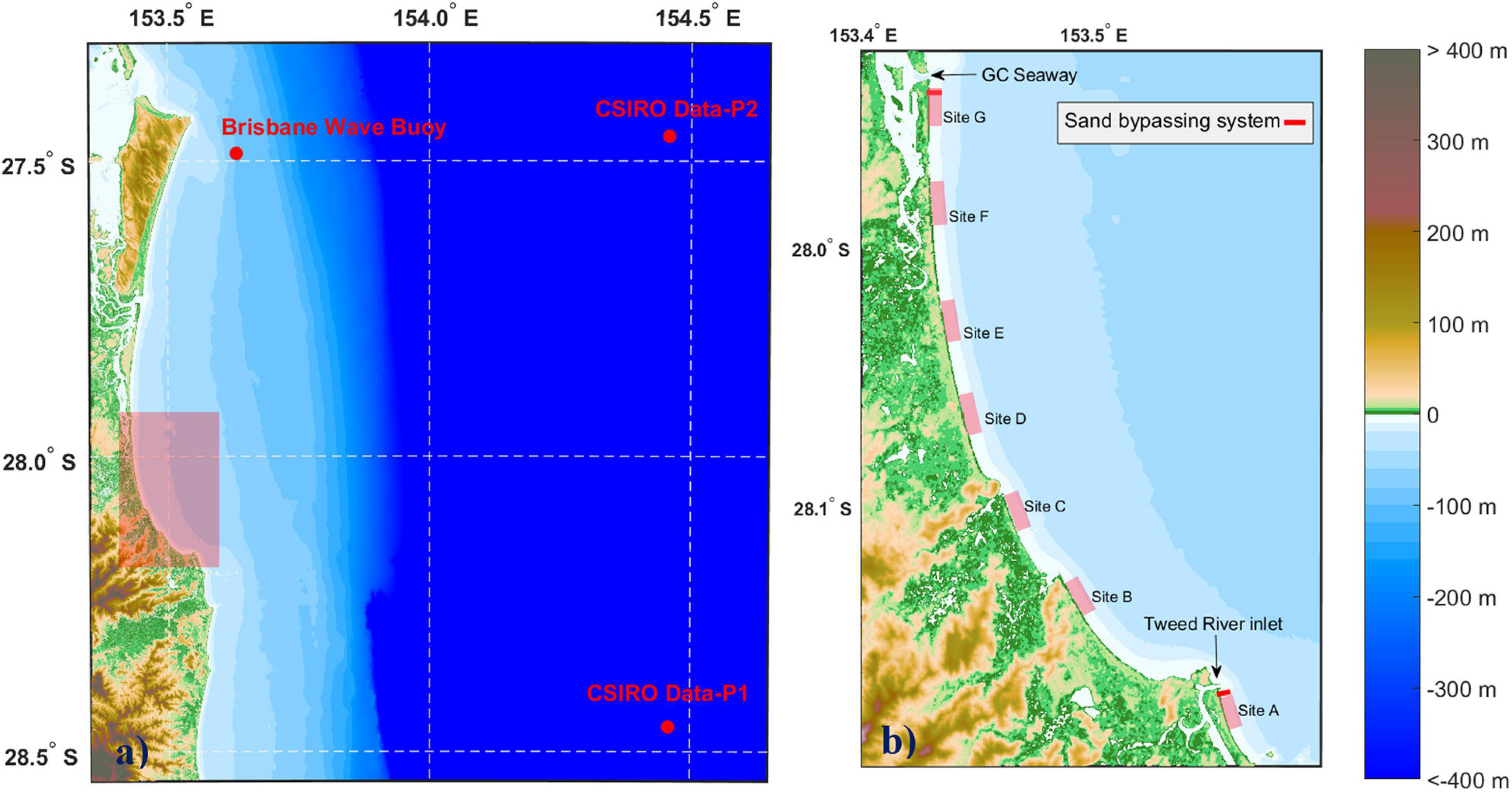
Figure 1. (a) Study area (highlighted); (b) Location of sites selected for LST projections (adopted from Zarifsanayei et al., 2022).
There are three distinct seasons for offshore wave climate systems in Gold Coast (City of Gold Coast, 2015): summer (December–May), winter (June–August), and spring (September–November). During the summer, the swell wave energy from east to south-easterly directions, approaches the coast. During the winter, the dominance of the highly energetic south to south-easterly swells, originating in the Southern Ocean, adds a considerable amount of energy to the system. Usually, the spring wave climate exhibits calmer conditions compared to the other seasons. However, in all seasons, stormy conditions can be observed. Also, locally generated wind-seas exist throughout the seasons.
The exposure of the GC coastline to wave climate, differs from south to north, mainly due to changes in the coastline orientation and refraction patterns (Vieira Da Silva et al., 2018). While the northern beaches are open east-facing coasts, the southern beaches are semi-embayed/sheltered regions, facing northeast to the north directions (Figure 1b). Hence, the northern GC is more exposed to south-easterly swell wave energy, and in the nearshore region, an increasing trend for wave height from south to north is conceivable. In this study, seven sites from south to north GC, were selected to investigate uncertainty in the LST projections (see Figure 1b). The sites are relatively far from headlands and coastal structures. Two sites in proximity of the sand bypassing systems (sites A and G), two sites in the semi-sheltered regions (sites B and C), one site located in middle of GC (site D) and two sites between the middle and north of GC (site E and F), were selected.
Methodology
Perspective of the Methodology
In order to investigate uncertainty in the projected wave driven sediment transport patterns, an ensemble modelling, consisting of two RCPs, eight GCM-Ws, and eight LST models is proposed. The estimations cover two time slices of 1979–2005 (baseline period), and 2081–2100 (far future). The methodology was structured in three phases which were estimation of wave forcing conditions, response of sediment transport models to the forcing conditions, and uncertainty quantification (Figure 2). As both original datasets and bias-corrected data were considered individually in this study (two separate ensembles), in aggregate, from each ensemble, 128 sets of results were obtained by which uncertainty of the LST projections was investigated.
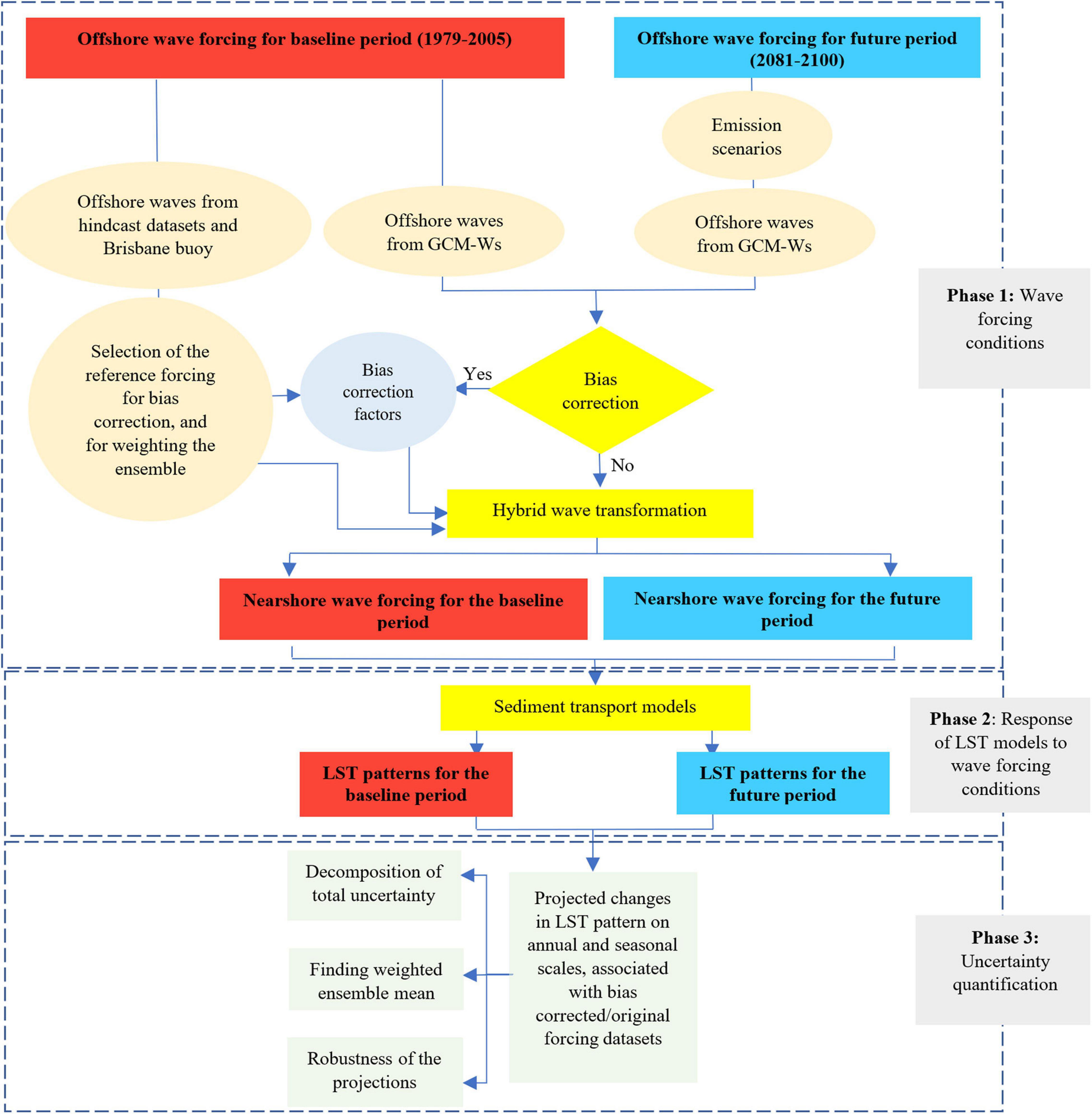
Figure 2. Flow chart of the methodology.
Wave Forcing Conditions
The Projected Offshore Waves
To decrease the computational costs of dynamical wave climate change projections, a subset of GCMs (not all of the available GCMs) is usually selected beforehand. Then, the GCMs outputs are introduced to wave modelling approaches (i.e., statistical, Camus et al., 2017; dynamical, Hemer and Trenham, 2016). Recently, CSIRO has attempted to project changes in wave climate on the global scale by forcing the spectral wave model WAVEWATCH III with the wind fields and sea ice fraction obtained from eight CMIP5 GCMs, including ACCESS1.0, BCC-CSM1.1, CNRM-CM5, GFDL-CM3, HadGEM2-ES, INMCM4, MIROC5, and MRI-CGCM3 (Hemer and Trenham, 2016). The criteria for choosing the GCMs were accessibility to the data, and their ability to reproduce the patterns of common climate variables (i.e., air temperature, precipitation, and sea-surface temperature) for a baseline period. The main features of the GCM-forced wave simulations (henceforth GCM-Ws) conducted by CSIRO can be found in Table 1. The CSIRO datasets have incorporated the uncertainties associated with emission scenarios and choice of GCMs while covering three time slices of 1979–2005 (as the baseline period), 2026–2045 (as the near future period), and 2081–2100 (far-future period). Moreover, the temporal resolution of the GCMW (i.e., 6 hourly) provides additional information to understand projected changes in the patterns of storm waves (Meucci et al., 2020). The main outputs of the GCM-Ws are integral parameters of total wave energy (i.e., Hs: significant wave height, Tp: peak wave period, and Dm: mean wave direction) and also the parameters associated with the partitions of wind-sea and swell. The patterns of the annual mean wave parameters (i.e., Hs, Dm) for baseline and future periods, obtained from the GCM-Ws datasets within the Coral Sea and Tasman Sea (the origins of wave energy at the offshore region of Gold Coast), can project the likely impacts of CC on offshore waves (see the Supplementary Material, Part A). Overall, the ensemble future projected annual mean wave patterns, compared to those of the present time, show a decrease in wave height (∼5%), and a slight rotation of waves toward east (∼5 deg anticlockwise) for offshore regions of southeast Queensland. Currently, the spatial resolution of the wave projections is quite coarse for regional and local studies, and therefore, the GCM-Ws should be downscaled. In this study, integral parameters of total wave energy (i.e., Hs, Tp, Dm) from the CSIRO ensemble of dynamic wave climate projections, for baseline (i.e., 1979–2005) and far future (i.e., 2081–2100) periods, were considered as the offshore waves of southeast Queensland. Figure 1a shows the geographical location of the nearest grids of GCM-Ws to the study area.
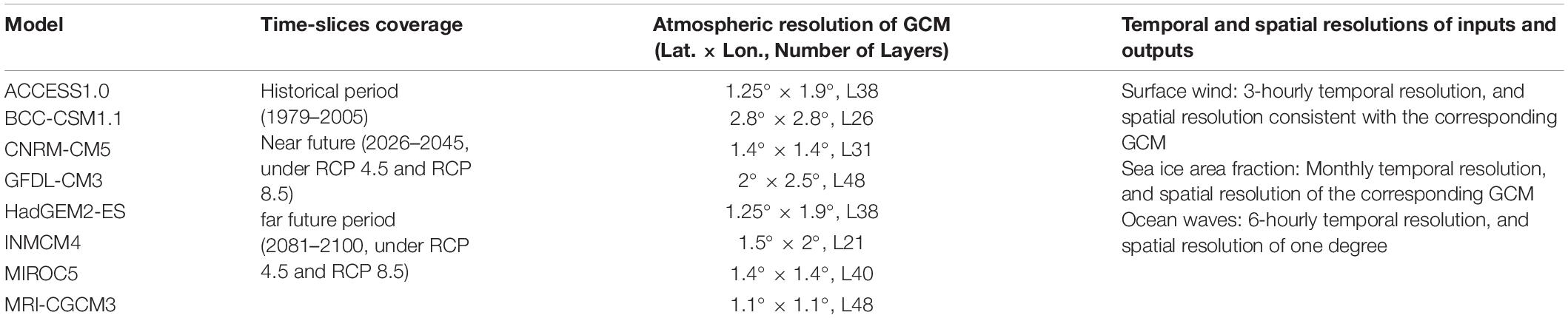
Table 1. Main features of GCM-forced wave simulations conducted by CSIRO.
Correction of the Biases of the Offshore Waves
The differences in the GCMs outputs for baseline and future periods are usually used in CC studies. However, the ability of GCMs to properly reproduce the historical climate (obtained from observations, measurements or modelling efforts like reanalyses or hindcasts) is a key step to assess the GCMs outputs. Generally, GCMs outputs can contain significant biases arising mainly from parametrization within the modelling frameworks (IPCC, 2014). These biases can also increase the uncertainty of GCM-Ws projections (Morim et al., 2018). To address this issue, bias correction (BC) methods have been employed so far to correct the systematic errors of GCMs outputs (e.g., Ranji et al., 2022) or even GCM-Ws (Lemos et al., 2020a,b). BC methods try to enhance the agreement between model simulations and observational/reference data for a historical time scale (baseline period). As the GCM data are not time coherent, the BC methods cannot be implemented on hourly timescales. Hence, the methods are time-independent, working with distributions/statics of the variables. A wide range of bias correction methods from the simple delta method (Hay et al., 2000) to more complicated ones based on quantile mapping (Amengual et al., 2012) has been developed in the literature. Applying BC methods in the context of CC is based on the assumption that the behaviour of biases detected in the GCMs data for the baseline period does not vary in time, and it remains the same for the future period.
Following Lemos et al. (2020b), in this study, correction approaches of Empirical Quantile Mapping (EQM) and Empirical Gumbel Quantile Mapping (EGQM) were adopted. The EQM applies a different correction factor to each quantile of the data by mapping the modelled empirical cumulative distribution functions (ECDF) to the reference ones. The quantiles are linearly spaced from 1st to 99th quantiles (qi = 1, 2, 3, …, 99, i = 1, …, nq, with nq = 99 quantiles). The EQM was applied to the parameter Dm, as follows:
The correction term X(qi) is calculated as the difference between the inverse ECDFDm of the reference dataset () and GCM-Ws (). DGCMWs–Dm and are the original and bias corrected Dm, respectively. Note that, the Dm was first transformed to zonal (u) and meridional (v) components, and each component was corrected individually using the abovementioned equations. The bias corrected u and v were used to reconstruct the parameter Dm.
The EGQM is a modified version of the EQM, in which quantiles are defined by a Standard Gumbel Distribution (SGD), providing a better representation for the upper tail of the data distribution. In total, 20 quantiles (nq = 20) ranging from 1st to 99.999th, were selected such as:
where qi is the quantile associated with the SGD. The rest of EGQM method is similar to the simple method of EQM (Eqs 1, 2). Since in the EGQM, more than 50 % of the selected quantiles are above 99th, the method focusses on correction of extreme conditions where higher biases are typically observed. The EGQM was applied to parameters Hs and Tp of GCM-Ws individually.
Performance of Original and Bias Corrected Datasets of Global Circulation Model-Driven Offshore Wave Datasets
To apply bias correction to GCM-Ws, first, a reference dataset is chosen. Here, the hindcast dataset of CAWCR (with three different spatial resolutions of 4, 10, and 24 min) along with the ERA5 reanalysis dataset were considered. Hence, CAWCR and ERA5 wave parameters from the nearest co-located grid points to Brisbane buoy were extracted and compared with the Brisbane Buoy data for the period 2000–2020. Finally, the CAWCR 24 min resolution hindcast was selected as the reference data (ground truth) for bias correction of GCM-Ws (hereafter Reference, see also Part A of Supplementary Material for more details).
For a qualitative comparison of GCM-Ws (before and after bias correction) with the reference dataset, the average of energy flux per direction, QQ plots (for parameter Hs), wave roses (Hs-Dm), and monthly mean patterns of wave parameters (Hs, Tp, and Dm) obtained from each GCMW offshore of Gold Coast were considered. For the quantitative comparison, the performance of each GCM to reproduce the patterns of Hs was evaluated against reference data using the following metrics: Bias (Eq. 5), PDF-score (Brands et al., 2011; Eq. 6), Arcsin–Mielke score (M-score; Hemer and Trenham, 2016; Eq. 7), Yule-Kendall skewness measure (YK; Lemos et al., 2020b; Eq. 8), all of which are defined below:
where j is the GCM-W number (1–8), N is the length of the timeseries, i is the index of the data, REF is the reference hindcast dataset (i.e., CAWCR 24 min).
The PDF-Score accounts for the area between empirical probability density functions (PDFs) of the reference data and each of the GCM-Ws. The score varies from 0 (showing no similarity) to 1 (perfect similarity). The PDF-Score was only applied to the parameter Hs of GCM-Ws.
The skills of GCM-Ws can also be assessed through the non-dimensional M-Score. The M-score ranges from negative values (a negative or zero value means no skill) to a maximum possible value of 1000.
As GCM-Ws are not time constrained to the reference data, all inputs of the M-Score formula are multi-year monthly means of Hs, Tp, and Dm.
The YK coefficient measures the skewness of GCM-Ws distributions, compared to those of the reference data. The skewness considers the relative positions of the quantiles (the 95th and 5th quantiles) with respect to the median (50th quantile). The YK measure was applied to the parameters of Hs and Tp parameters of GCM-Ws.
Wave Transformation
The Hs, Tp, and Dm parameters, extracted from one offshore grid point of GCM-Ws and CAWCR 24 min datasets (CSIRO-P1 in Figure 1a), were utilized to reconstruct a single-peak spectrum at the boundary of a spectral wave model (i.e., Mike 21 SW; DHI, 2017) which was previously used and calibrated for the study area (Splinter et al., 2012; Zarifsanayei et al., 2022; see also Part D of Supplementary Material). The offshore waves were then propagated to nearshore regions under the stationary mode of wave simulation. The shape of the spectrum at the open boundary of the wave model was reconstructed using a JONSWAP spectrum (with a peak enhancement factor of 3.3) for frequency distribution and cosn spectrum for directional distribution of wave energy. No local wind forcing was considered for wave transformation as the GCMs used in this study provide only coarse resolution data, missing the detailed local wind patterns.
Employing Mike 21 SW to transfer a large amount of data (over 750,000 outputs of 6-hourly wave events) to nearshore zones is not feasible with reasonable computational costs. Hence, following Antolínez et al. (2019), a hybrid approach was adopted. The hybrid method resulted in a surrogate model by which the whole time series of nearshore waves were reconstructed with significantly reduced computational costs and promising accuracy. In contrast to many reduction-forcing techniques (e.g., energy flux method, k-mean; de Queiroz et al., 2019), reconstruction of the whole timeseries of nearshore waves is more in line with the aims of this study, as it decreases the risk of capturing artificial climate change signals being caused due to improper condensing of the forcing conditions. The steps of the hybrid transformation of waves are outlined in Figure 3.
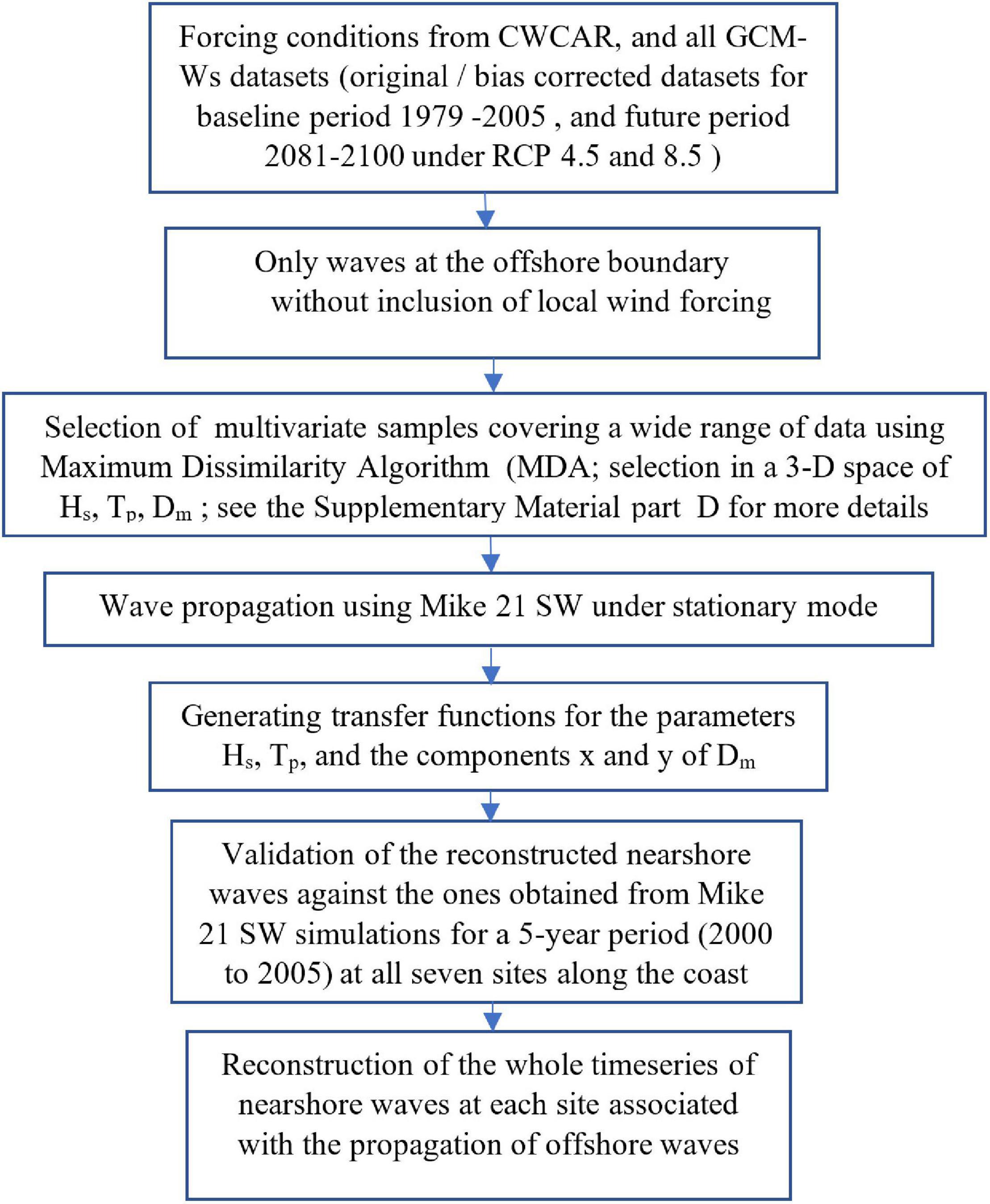
Figure 3. Flow chart of nearshore wave reconstruction.
Response of Sediment Transport Models to the Nearshore Forcing Conditions
Two classes of sediment transport models, including process-based model and bulk formulae were employed to avoid biases resulting from the use of a single class of models for projection of LST patterns. The bulk formuale were CERC (Mil-Homens et al., 2013; hereafter MC), modified Kamphuis (Mil-Homens et al., 2013; hereafter MK), van Rijn (van Rijn, 2014; hereafter V) and Shaeri et al., 2020 (hereafter S). The process-based model DHI-LITPACK (Kristensen et al., 2016) under four different set-ups (hereafter DHI-S1, DHI-S2- DHI-S3, DHI-S4) were also employed. The models were previously run under wave forcing obtained from Gold Coast Wave buoy (near site G located in water depth 17 m, covering the time slice 2008–2020), and then calibrated to reproduce a target annual mean net LST rate of 635,000 m3/year for site G (see Supplementary Material, Part E). The rate was consistent with observations at site G, where a sand bypassing system has been operational since 1986 (GCCM, 2017). Hence, a reliable estimate for LST was linked to a reliable forcing dataset for calibration of the LST models (see Zarifsanayei et al., 2022 for more details). All settings used for the calibration of the LST models, including the beach slope, the shape of coastal profiles, shoreline orientation, etc. were kept untouched for the LST projections of this study. The response of calibrated LST models to the nearshore wave forcing associated with the offshore reference forcing (i.e., CAWCR at 24 min spatial resolution offshore and transferred to the nearshore zone by the surrogate wave model) was checked at all sites to ensure that the calibrated LST models could present relatively consistent patterns on monthly and annual scales (see Figure 4 for site G). The inter- and intra-annual LST patterns along the coast were then used as the the refrence LST data.
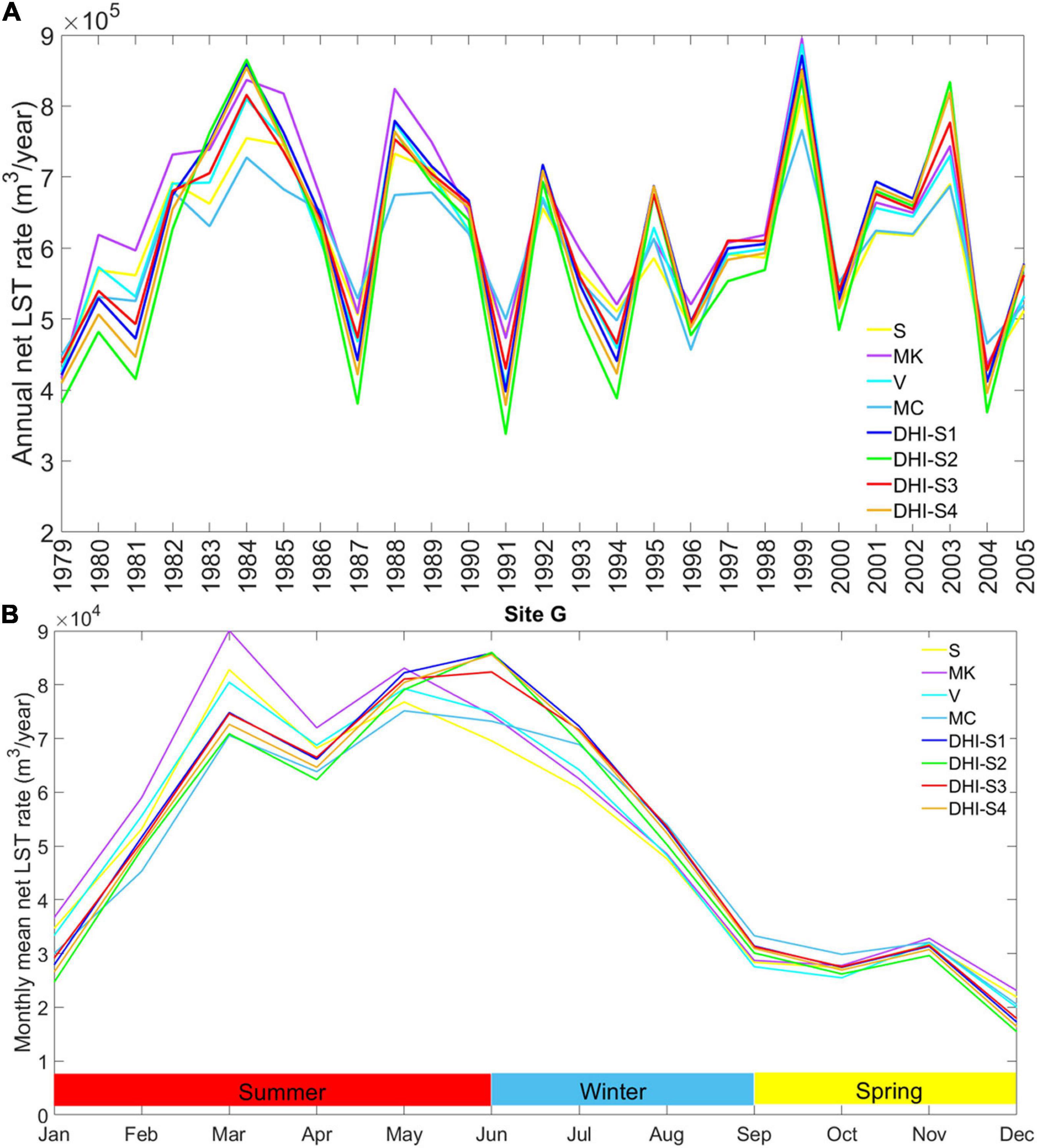
Figure 4. (A) Inter-annual and (B) Intra-annual response of the calibrated LST models to the reference forcing conditions.
At each site along the coast, the response of the calibrated LST models to nearshore wave forcing conditions associated with each set of GCM-Ws datasets, were stored in a 6 hourly timeseries format. Then, the relative future projected changes in the net LST rate on annual/seasonal scales were simply computed as follows:
where △LSTm is the projected changes in LST rate represented by mth simulation (member) of the ensemble (in total, for each ensemble, 128 projections exist due to the combination of two RCPs, eight datasets of GCM-Ws, and eight LST models), LSTF(LSTMl, GCMgf, RCPr) is the future-period rate of LST obtained from the combination of the lth LST model (LSTM) with forcing conditions associated with the gth dataset of the GCM-Ws projections under the rth RCP (i.e., 4.5/8.5), and LSTB(LSTMl, GCMg) is the baseline-period rate of LST obtained from the combination of the lth LSTM with forcing conditions associated with the gth dataset of the GCM-Ws.
Quantification of Uncertainty
For each site along the coast, the total uncertainty of LST projections is obtained from the following path: working with original or bias corrected datasets of offshore waves projected by different GCM-Ws under two RCPs, transferring the offshore waves to nearshore through the surrogate wave model, and then forcing the calibrated LST models accordingly. Following Zarifsanayei et al. (2022), the total uncertainty of the projections (i.e., variation of the results), for each site individually, was also decomposed into its sources (i.e., RCPs, GCM-Ws, LSTMs) and their interactions by using ANOVA model.
To find the ensemble mean, a simplified method for weighting the members of the ensemble was adopted (e.g., Sanderson et al., 2015). Given the baseline period 1979–2005, the following criteria were considered:
(a) Annual mean LST rates of each ensemble member compared to the reference LST data.
(b) Equilibrium shoreline orientation (i.e., the orientation for which annual mean net LST rate is zero) obtained from each ensemble member, compared to the reference patterns.
(c) Consistency of the net LST patterns along the coast, obtained from each ensemble member, compared to the respective reference patterns of LST along the coast.
To meet the last criterion, the first two criteria were considered together for four sites along the coast (i.e., sites A, B, D, and G as the representative of different types of coastal sediment sub-cells along the coast). Then, the following steps were taken to assign a weight to each member of the ensembles:
(a) Annual LST rates (ALR) were normalized (by considering maximum and minimum of the annual mean LST rates at the aforementioned sites).
(b) Equilibrium shoreline orientations (EQO) were normalized (by considering maximum and minimum of equilibrium shoreline orientations at the aforementioned sites).
(c) For each ensemble member a distance (here, a Euclidian distance in an 8-dimensional space due to considering four sites and two variables ALR and EQO) between two points (one point for the ensemble member and one point as the reference) was calculated as follows:
where Distancem refers to the distance assigned to ensemble member m.
(d) Distances were then used in a simple form according to the inverse distance weighting concept as follows:
where Scorem is the score of the ensemble member m, and Wm is the weight attributed to that ensemble member. Note that for weighting purposes, each ensemble has 64 members for the baseline period (a combination of eight datasets of GCM-Ws and eight LST models). While for projections of changes in LST patterns, each ensemble has 128 members (a combination of two RCPs, eight datasets of GCM-Ws, and eight LST models).
Another important aspect of uncertainty quantification is the investigation of the degree of the ensemble members’ consensus on the projected changes. The criteria to check the robustness of the projections normally revolve around finding the ratio of the signal (from the externally forced changes) to noise (from internally forced changes). Two methods were used to investigate the robustness of the projected changes in LST rates on the annual and seasonal scales.
In the first one, the straight forward approach of Hawkins and Sutton (2009) was adopted. To do so, the robustness of the projected changes in LST rates was determined via the inverse of fractional uncertainty associated with 90% confidence level (i.e., signal-to-noise ratio), as follows:
where Ro stands for robustness of projections (if Ro > 1 the projections are robust), Meanw is the weighted ensemble mean, and Varw is the total weighted variance of the projected changes in LST rates.
In the second approach, following Tebaldi et al. (2011), the level of consensus on the significance of changes was determined. In doing so, the LST rates projected by each of the ensemble members were introduced to a t-test that checks the variances and means between the LST rates associated with the present and future periods. In this way, each ensemble member showing a significant change was identified. If less than 50% of the members exhibited a significant change, the projections were not considered robust. If more than 50% of the ensemble members reported a significant change, these members were selected, then the agreement on the sign of the projected changes (i.e., increase, + and decrease, –) was also tested by the following criterion: if more than 80% of the selected members agreed on the sign of the changes the projections were considered robust, otherwise the projections were not robust.
Results and Discussion
The approach by which offshore waves are used at the boundary of the spectral wave model, has a great impact on the projected nearshore wave patterns. Hence, first, the following tests were conducted to understand the impact of some issues on LST patterns: applying offshore waves uniformly or non-uniformly along the boundary of the wave model and directional standard deviation parameter (DSD). To do so, a 5-year time slice of wave data (covering 2000–2005), obtained from the Reference-W, was selected to force the spectral wave model. Then, the nearshore waves at each site were calculated and introduced to the LST models. Monthly means of LST rate was used as the criterion for the comparisons. The results showed that given the resolutions of the GCM-Ws, in terms of time and space, it can be assumed that waves at offshore region, are uniform, and can be transferred to the nearshore region under a stationary assumption of wave transformation (see Supplementary Material, Part B for details of the tests).
For the initial assessment of the GCM-Ws, for each dataset of GCM-Ws during the baseline period, the average of wave energy flux (WEF), approaching the coast from different directions, was plotted on a polar coordinate system (Figures 5A,B), using a 10° bin. The comparison of the average of WEF presented by the original datasets with that of the reference data, clearly indicates that most of GCM-W datasets (except MIROC5 and MRI-CGCM3) are not successful in capturing the expected patterns of WEF that predominate within the S to SE directions (Figure 5A, see also Supplementary Material, Part C1). Among the eight GCM-W datasets, BCC-CSM1.1-driven waves show the greatest bias in wave energy patterns, predominating from E. The original datasets of GCM-Ws exhibit biases from –0.2 to –0.5 m for the Hs and –1 to 1 s for the Tp (Figure 6A). The GCM-Ws associated with MRI-CGCM3 and MIROC5 show the lowest biases. The analysis of the original datasets of GCM-Ws indicates large biases for the Dm, ranging from –27 to –10 degrees, with the largest found for the BCC-CSM1.1 (Figure 6B). Such biases could be mainly due to the coarse spatial resolutions of the wind forcing- extracted from the corresponding GCMs- used for projection of offshore waves. Applying the bias correction has profoundly improved the patterns of offshore WEF (Figure 5B). However, still, the BCC-CSM1.1-driven waves show a recognizable bias for the average of the WEF patterns. Figures 5C,D show that the bias correction could effectively decrease the biases along the upper tail of the Hs quartiles. Improvement of the PDF-Score for Hs also acknowledges the functionality of the bias correction approach (Figures 5E,F). The PDFs of the original and bias corrected Dm imply that the corrected waves were diverted from E direction to S and SE directions (Figures 5G,H). By applying the bias correction to the GCM-Ws, the YK measures for the Hs and Tp were shifted nearly to zero, implying that the distributions of the parameters (in terms of skewness) became similar to those of the reference dataset (i.e., CAWCR), after bias correction (Figure 6D). Additionally, the M-Scores increased dramatically after bias correction, indicating the effectiveness of the bias-correction methods (Figure 6C). Overall, a consistent improvement in the accuracy of all bias-corrected wave datasets, was observed.
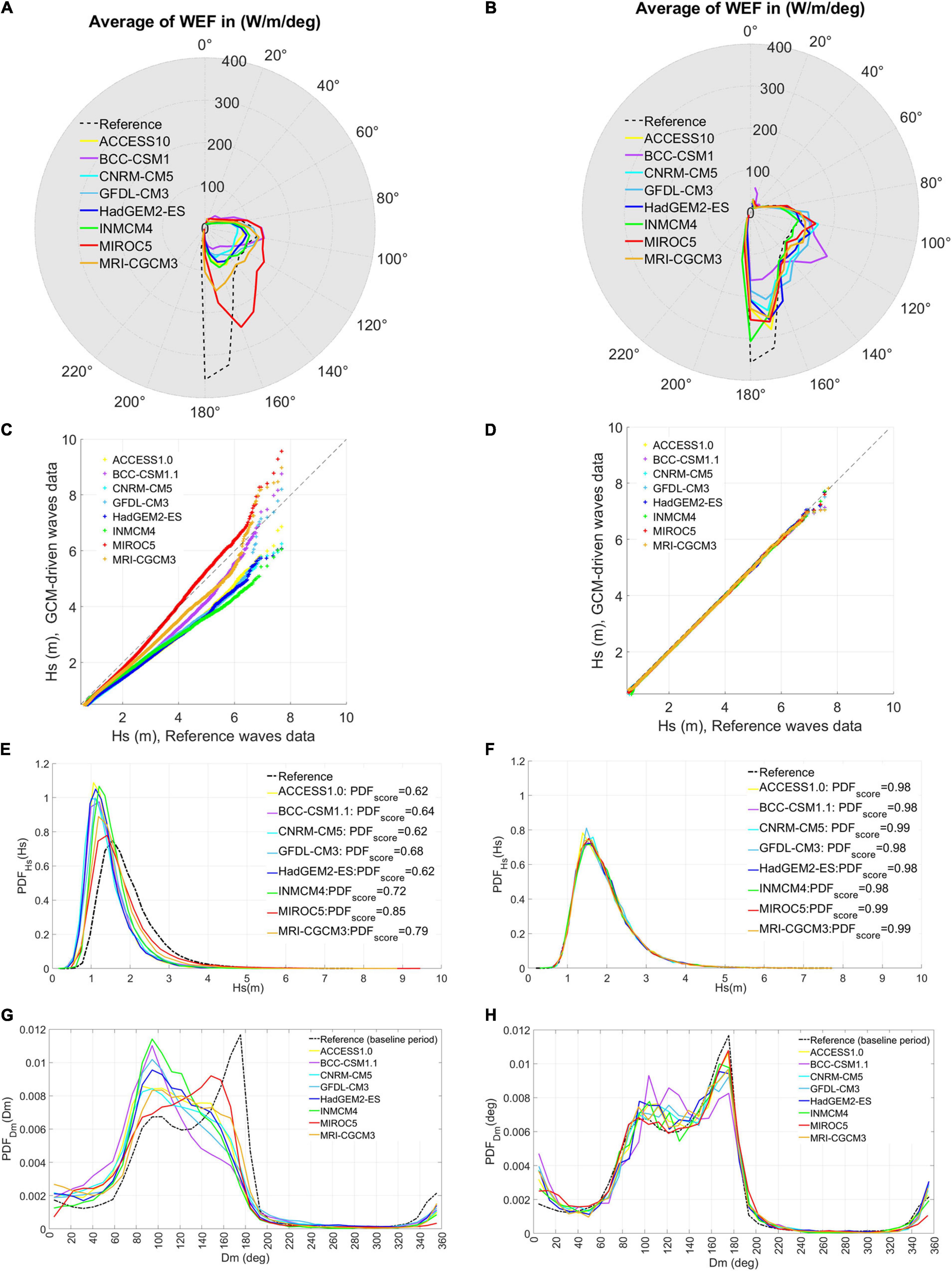
Figure 5. Comparison of bias-corrected and original datasets of GCM-Ws for the baseline period 1979–2005. (A) Average of wave energy flux presented by the original datasets. (B) Average of wave energy flux presented by the bias-corrected datasets. (C) QQ plots for Hs of the original datasets. (D) QQ plots for Hs of the bias-corrected datasets. (E) PDF for Hs of the original datasets. (F) PDF for Hs of the bias-corrected datasets. (G) PDF for Dm of the original datasets. (H) PDF for Dm of the bias-corrected datasets.
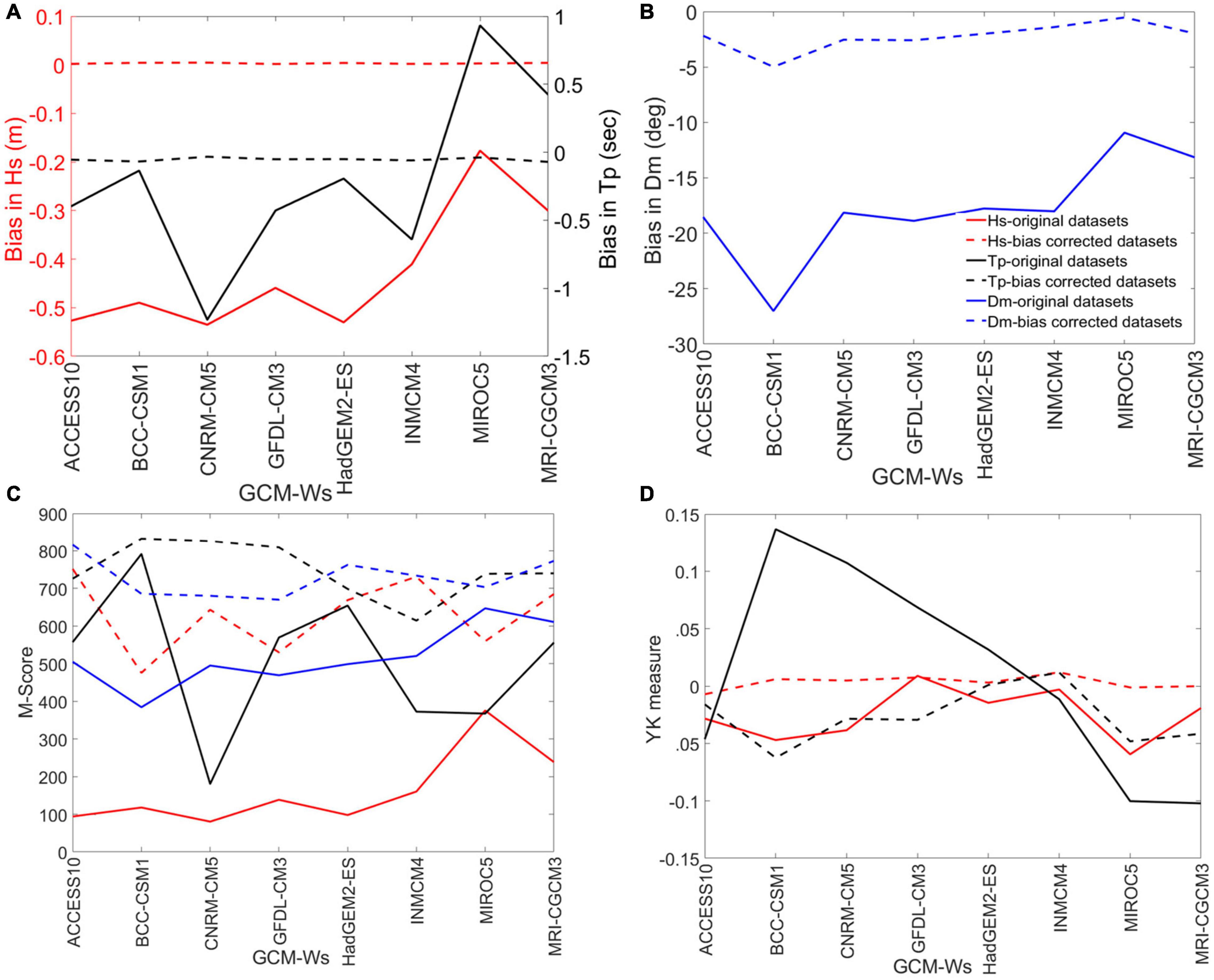
Figure 6. Comparison of the bias corrected and the original datasets in terms of (A) Biases in Hs and Tp; (B) Biases in Dm; (C) M-Scores; (D) YK measures.
As the bias correction methods are purely mathematic ones (based on present climate statistics), rather than physics-based approaches, their use always might yield the risk of manipulating the CC signals of the original dataset of any kind (Maraun, 2016). Hence, the signals obtained from both types of forcing datasets should be compared to understand whether the bias correction has caused artificial changes or not. In doing so, the projected offshore waves monthly and annual means were calculated to be compared qualitatively. The results show that in terms of the projected changes, in monthly and annual mean wave parameters, there is a general agreement between the original and bias-corrected forcing datasets. However, on the annual scale, occasionally, the bias correction has reduced the projected changes in offshore wave parameters, particularly for parameter Dm (see Supplementary Material, Part C2). Moreover, the bias correction method of EGQM (used for Hs) sometimes changes the signals of CC for the upper tail of Hs distributions. This is due to the properties of the method, which focuses on correcting the upper quantiles. A prime example of such a condition was observed by comparing the projected changes in Hs presented by the original dataset of BCC-CSM1.1 with those of the bias-corrected wave dataset (see Supplementary Material, Part C2).
All of the original and bias corrected wave datasets were then transferred to the nearshore sites using the surrogate wave model. The reconstructed time series of nearshore waves were used to calculate the monthly means of the alongshore component of wave energy for the baseline period 1979–2005. The results indicate that applying the bias corrections leads to the nearshore wave energy patterns that are more consistent with the ones associated with the reference forcing (see Supplementary Material, Part D). The combination of different nearshore forcing conditions obtained from the transformation of offshore waves of the original/bias corrected datasets (for the baseline and future periods), with different LST models resulted in a large ensemble whose members have different levels of reliability. Hence, to evaluate the performance of each ensemble member, the patterns of LST along the coast presented by each ensemble member for the baseline period 1979–2005, were compared with the ones obtained from the response of the calibrated LST models to the reference forcing (see Supplementary Material, Part E). As mentioned before, a weighting scheme was also used accordingly. The annual mean LST rates along the coast associated with the use of the bias-corrected forcing conditions implied that the bias correction was successful in reducing the uncertainty of LST estimates for the baseline period (see Figure 7). This issue was expected from the impact of bias correction on S-Phi curves which show the relationship between shoreline orientation and LST rate of each site (see S-Phi curves of site D at Supplementary Material, Part E). As shown in Figure 7B, the weighted ensemble mean for the annual mean LST rates associated with using the bias-corrected forcing conditions is close to the reference patterns of LST rate. Whereas as shown in Figure 7A, the weighted ensemble mean associated with using the original forcing datasets is quite different from the reference LST patterns. Also, when the original forcing conditions are used, the ranges of uncertainty in estimation of LST rates are very large. Since having a reasonable pattern for LST rates along the coast is a pre-requisite for coastal erosion studies, using the bias-corrected wave forcing conditions might be more reasonable for such studies, instead of using the original datasets.
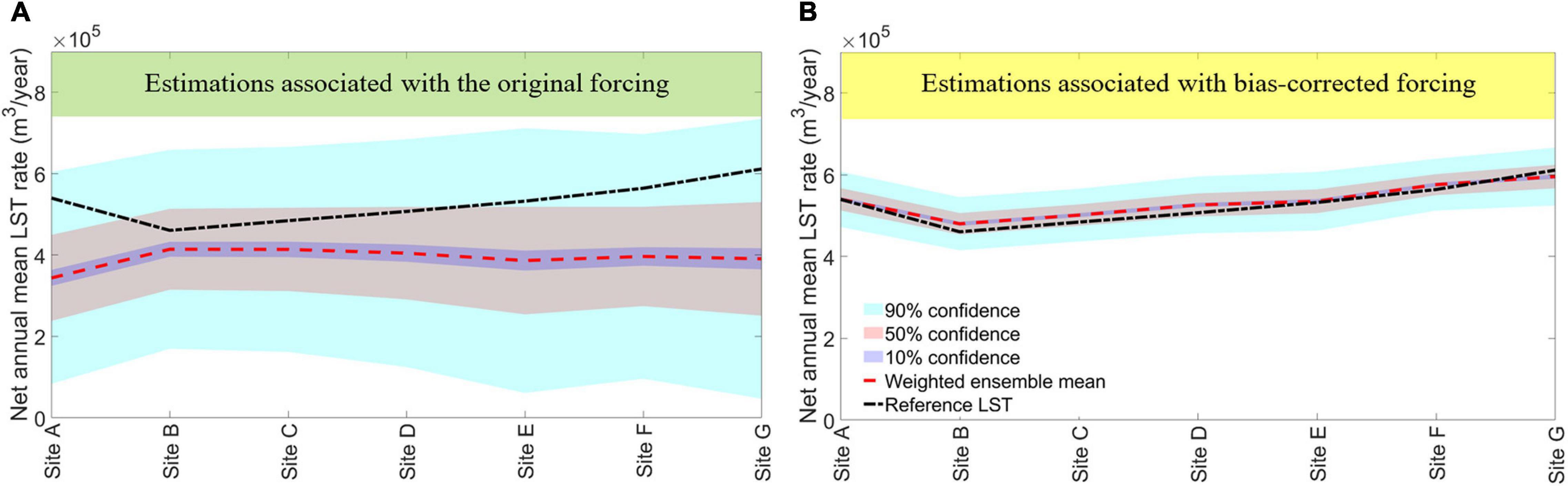
Figure 7. Annual mean LST rates for the baseline period 1979–2005 associated with (A) bias corrected forcing conditions and (B) the original ones; Reference LST was obtained from the average response of the calibrated LST models to the reference forcing; Highlighted areas indicate the uncertainty ranges for LST estimates.
To project the future patterns of sediment transport, uncertainty issues should be accounted for. Different responses of each class of the calibrated LST models (i.e., process-based and bulk formula) to new forcing conditions -the ones such as the original datasets of GCM-Ws that were not used for calibration of the LST models - can be one of the sources of uncertainty in the projections. For instance, the violin plots of the annual LST rates associated with forcing conditions of MRI-CGCM3 at site D (Figure 8), show how the LST projections on the annual scale can be impacted by changes in distribution of the LST rates obtained from different models. Such a discrepancy might be important for long-term coastal erosion studies in the context of climate change, where bulk formulae are usually utilized (e.g., Roelvink et al., 2020; Alvarez-Cuesta et al., 2021).
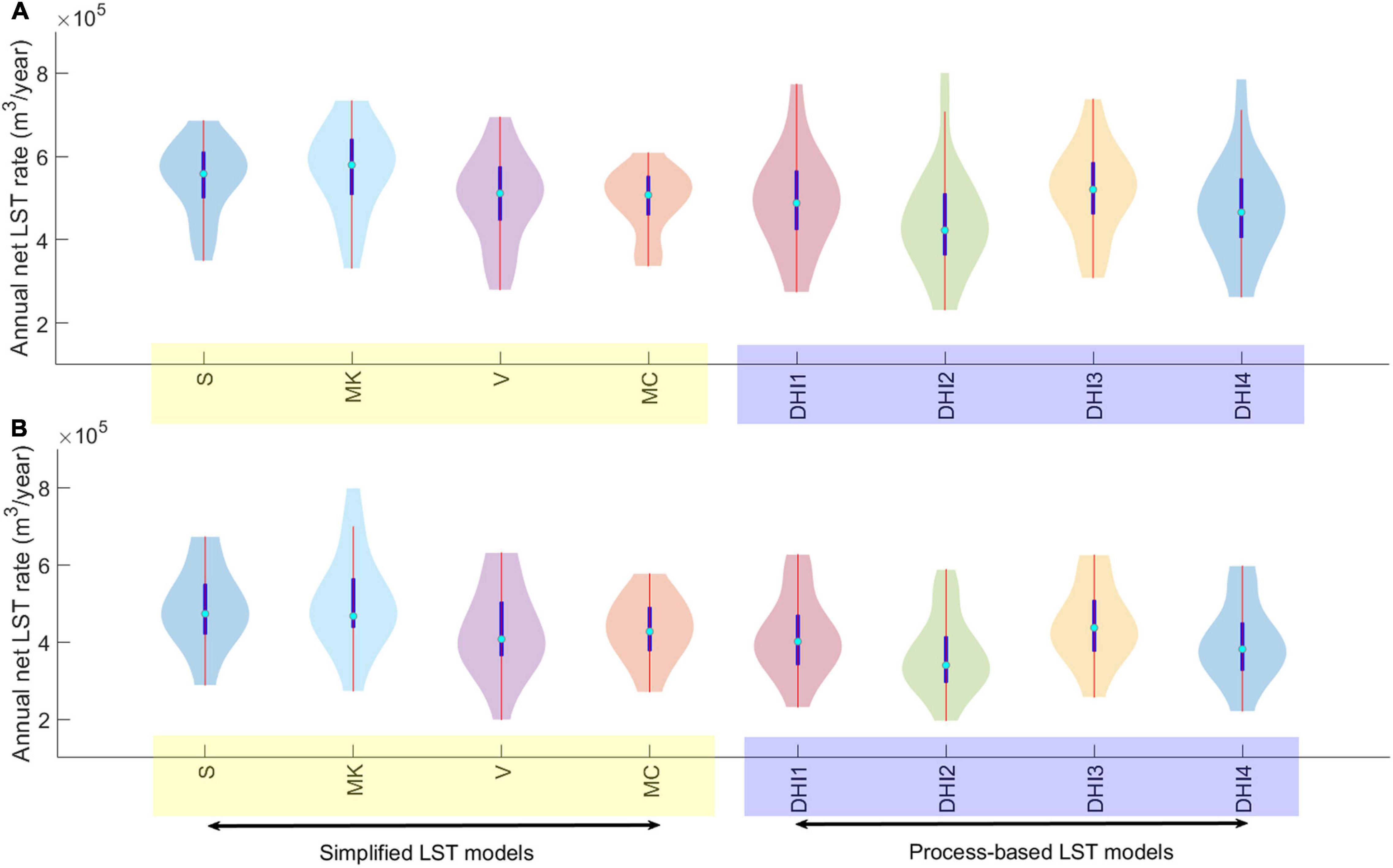
Figure 8. Violin plots of the response of different LST modes to the dataset of MRI-CGCM3 driven waves at site D during (A) the baseline period and (B) the future period (under RCP 4.5). The violin plot shaded area is the approximation of the probability density function (PDF) through a kernel density estimation (KDE), while the remaining information corresponds with that of a boxplot. Bias-corrected forcing conditions were used for the plots.
Although the choice of LST models seems to be important for the projections, the interaction of GCM-Ws and emission scenarios also contributes to the uncertainty of the projections (e.g., Yip et al., 2011). As illustrated in Figure 9, the use of some GCM-Ws (e.g., MIROC5 and GFDL-CM3) under different emission scenarios can even alter the sign (i.e., increase or decrease) of the projected changes in LST. Such interactions can challenge the reliability of any coastal sediment transport projections, conducted by arbitrarily choosing the GCM-Ws forcing datasets and emission scenarios (e.g., Dastgheib et al., 2016; O’Grady et al., 2019; Chowdhury et al., 2020). Apart from the aforementioned points, it seems that applying bias corrections could sometimes slightly manipulate the patterns of the LST projections under different emission scenarios, compared to those of the original forcing datasets (see Figure 9, the projections associated with BCC-CSM1.1 and ACCESS1.0 forcing conditions at site G). More graphs indicating the bias correction impacts on manipulating the trends of LST patterns can be found in Supplementary Material, Part F.
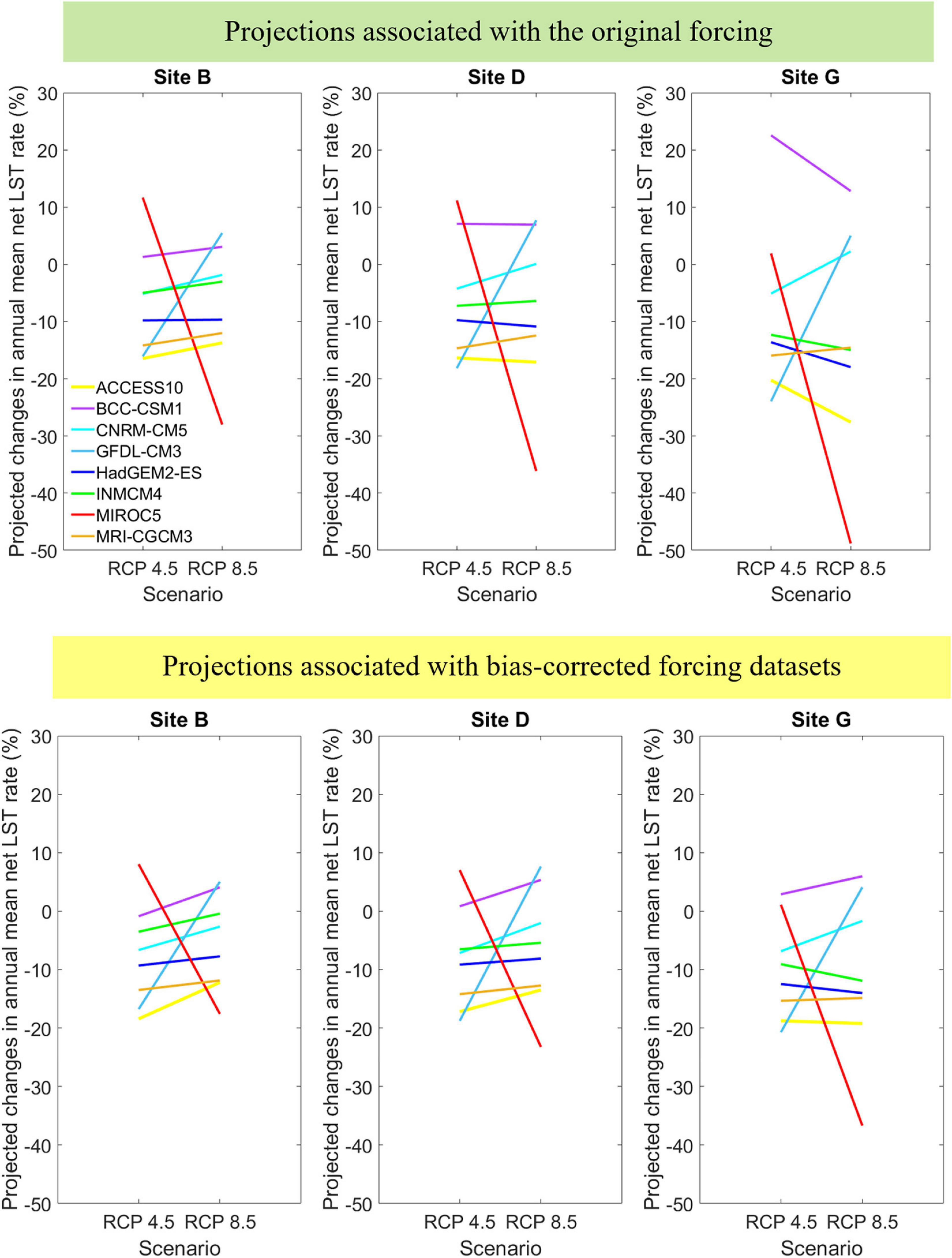
Figure 9. The role of interactions of GCM-Ws with emission scenarios on the projection of LST rates; Projections associated with using the original forcing datasets (top panel) and bias-corrected datasets (bottom panel); The projected changes in LST rate, here, were obtained from the average of all LST models’ outputs.
As mentioned before, the cascade of uncertainty (Le Cozannet et al., 2016; Toimil et al., 2021), was considered to quantify uncertainty of the projected changes in net LST patterns for each site along the coast. For instance, if offshore wave forcing associated with GCM-W #3 under RCP4.5 is used without bias correction, and then transferred to site G and introduced to LST model #1, meagre change (∼0%) in future net annual mean LST rate are observed compared to its corresponding baseline LST rate (see the magenta path in Figure 10A). Using the variance-based method of ANOVA, the total uncertainty of the projected changes in annual LST rate (at each site) was decomposed into main sources, including emissions scenarios, GCM-Ws, LST models, as well as their non-linear interactions. To enhance the accuracy of the uncertainty decomposition, following Bosshard et al. (2013), a subsampling technique was also employed. Each subsampling consisted of 8 members (i.e., a combination of two RCPs, two GCM-Ws, and two LST models). In aggregate, 784 subsamples were used to calculate the mean unbiased estimate of total uncertainty fractions (i.e., the averages obtained from all subsamples) attributable to each source (Figures 10B,C). It should be noted that the ANOVA is sensitive to the subsampling approaches (Wang et al., 2020); in this regard, the reader is referred to the Supplementary Material, Part G for further discussion. In all sites, the contribution of emission scenario uncertainty (alone) to total uncertainty is between 10 and 20%. Note that a part of this contribution is also masked by a significant non-linear interaction of emission scenario and GCM-Ws (∼25%). The contribution of GCM-Ws to total uncertainty is very large (greater than 40%), accentuating that a wide range of changes in the forcing conditions was captured by the projected offshore wave datasets of CSIRO. The contribution of LST model uncertainty is less than 15% of total uncertainty (Figures 10B,C). Additionally, the non-linear interaction of LST models and GCM-Ws is not significant (3–7%), and the rest of the non-linear interactions do not have conspicuous contributions to total uncertainty. Applying ANOVA to the variances of the LST projections, associated with the bias corrected forcing dataset, can probably lead to more consistent patterns of uncertainty attribution along the coast, compared to those of the original forcing datasets. Overall, in the case of applying/not applying the bias corrections, more than 75% of the total uncertainty of the LST projections is related to the uncertainty of the forcing conditions (i.e., the selection of RCPs and GCM-Ws, and interaction of scenarios and GCM-Ws).
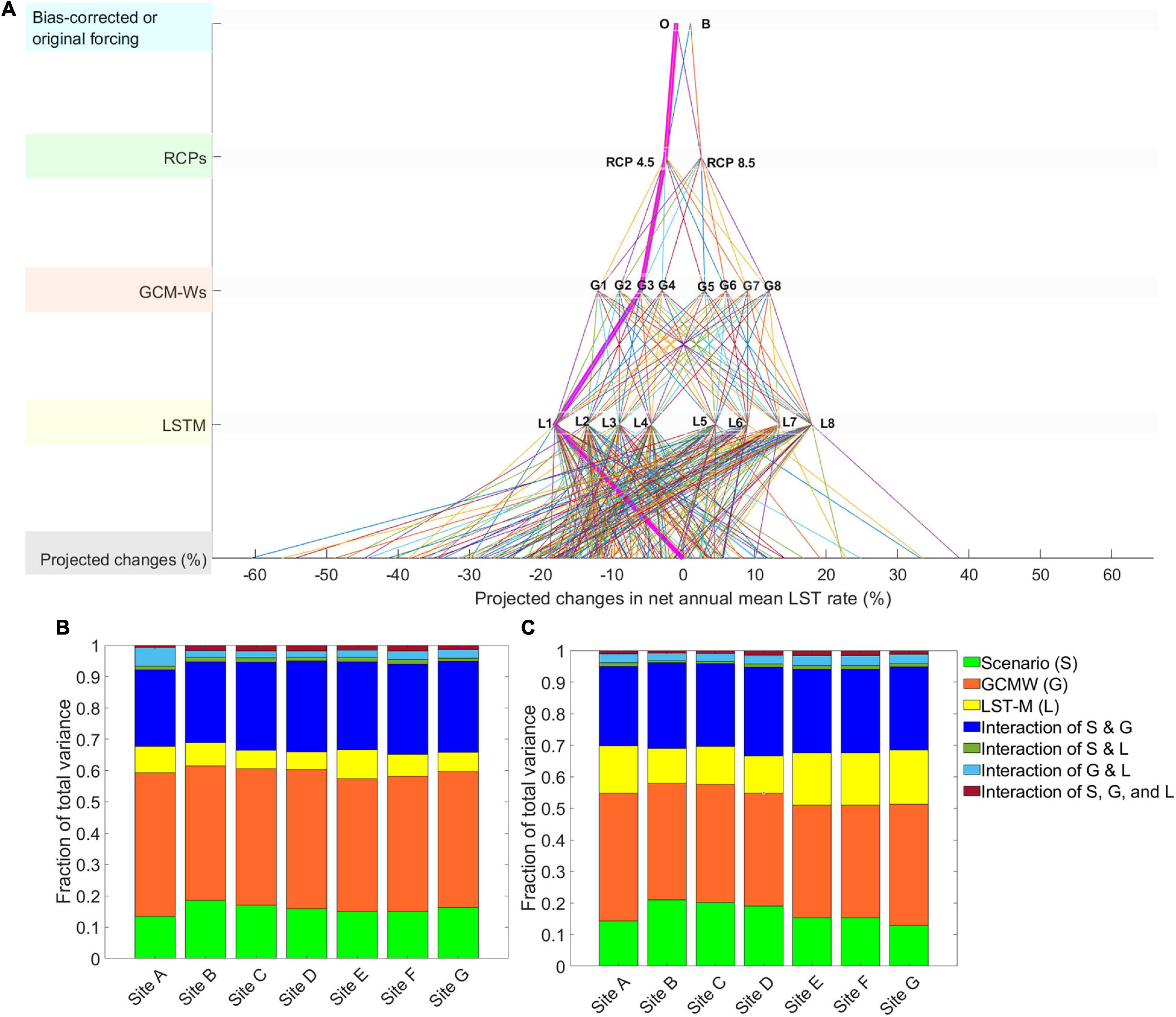
Figure 10. Quantification of uncertainty contribution; (A) Cascade of uncertainty in the projected changes in net annual mean LST rate at site G; Decomposition of the total uncertainty at all sites, associated with using (B) the original and (C) the bias corrected forcing conditions.
Using the outputs of the ensembles, the confidence intervals for the projected changes in net annual mean LST rate, were calculated. As shown in Figure 11, under RCP 4.5, from both ensembles, less than 10% decrease in the net LST rate is projected by the weighted ensemble mean. Under RCP 8.5, a wider range of uncertainty, compared to that of RCP 4.5, is captured. The weighted ensemble mean shows less than 20% decrease in the projected changes in net annual mean LST rate, and the projected changes associated with the original forcing is relatively different from those of the bias corrected forcing. Apart from that, the range of the uncertainty at site A, due to the large sensitivity of LST (at this site) to changes in wave direction, is larger than those of others (Zarifsanayei et al., 2022). Compared to the other sites, usually at the semi-sheltered sites (i.e., sites B, and C), a lower range of uncertainty is observed. Almost at all sites, when using bias-corrected or original forcing conditions, it seems that the difference between ensemble mean and standard deviation of the projected changes in annual LST rate, is large, questioning the robustness of the projections. However, still, all ensemble members consistently agreed that the future direction of the net LST on the annual scale will remain northward for all sites (see Supplementary Material, Part F).
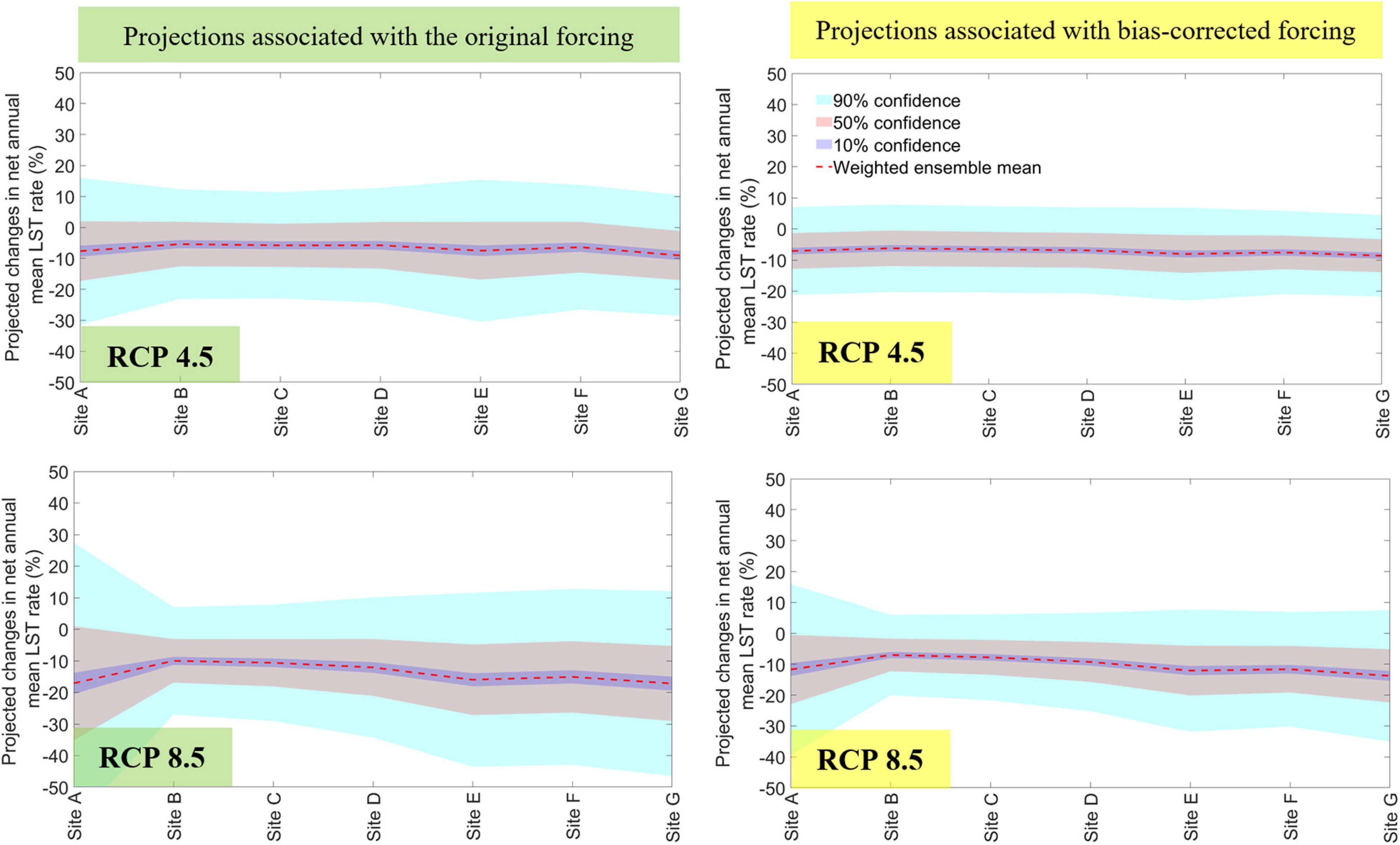
Figure 11. Projected changes in net annual mean LST rate associated with the original datasets of forcing conditions (left panel), and bias corrected ones (right panel).
Comparing the panels of Figure 11, it can be concluded that use of the bias-corrected forcing conditions has narrowed the uncertainty of annual LST projections to some extent. However, the uncertainty ranges are still quite large due to the following reasons. First, the bias correction methods applied the same correction factors to the forcing conditions of baseline and future periods, and as a result, the roles of the correction factors were probably less significant when the relative changes in LST rates were calculated. Additionally, the correction methods probably have not added remarkable artificial signals to the original forcing conditions (as discussed before), preserving a part of the original uncertainty.
The LST projections were also carried out on the seasonal scales, given three distinct seasons of summer, winter, and spring. The net seasonal mean LST rates for some of the ensembles’ members, during the baseline period, were close to zero, and that could yield an unreasonably large magnitude for the projected changes in seasonal net LST rates (e.g., some members projected 300% changes in net LST rate during spring). Hence, the seasonal LST rates were calculated for northward and southward directions, individually. To find the role of northward/southward LST in the long-term annual LST rate; the seasonal mean LST rates for each ensemble member during the baseline period, individually, were scaled according to gross annual mean LST rates. Results show that, on average, for all sites, ∼87% of the time of the year (i.e., ∼%52 in summer, ∼ 22% in winter, and ∼13% in spring), the LST direction is toward the north, and 13% of annual gross LST (i.e., ∼4% in summer, 3% in winter, and 5% in spring) belongs to the southward LST (see Supplementary Material, Part H for more details).
The projected changes in seasonal mean LST rates, for each direction of LST (northward/southward), were obtained from the relative difference of seasonal LST rates between the future and baseline periods. The weighthed ensemble mean, associated with using the original forcing, on the seasonal scales and under RCP 8.5, projected a maximum of 13, 22, and 10% decreases in northward LST rates during summer, winter and spring seasons, respectively (Figure 12, left panel). On the other hand, the weigthed ensemble mean, associated with the bias-corrected forcing conditions, under RCP 8.5, projected 10, 15, and 5% maximum decreases in northward LST rates for the same seasons (Figure 12, right panel). Although some changes in the southward LST rates are also observed (see Supplementary Material, Part I), these changes will not have a significant influence on changing the long-term annual patterns of the LST rate. Because, as mentioned before, the southward LST rates have a small contribution to annual gross LST rates. More graphs and explanations related to seasonal LST projections can be found in Supplementary Material, Part I.
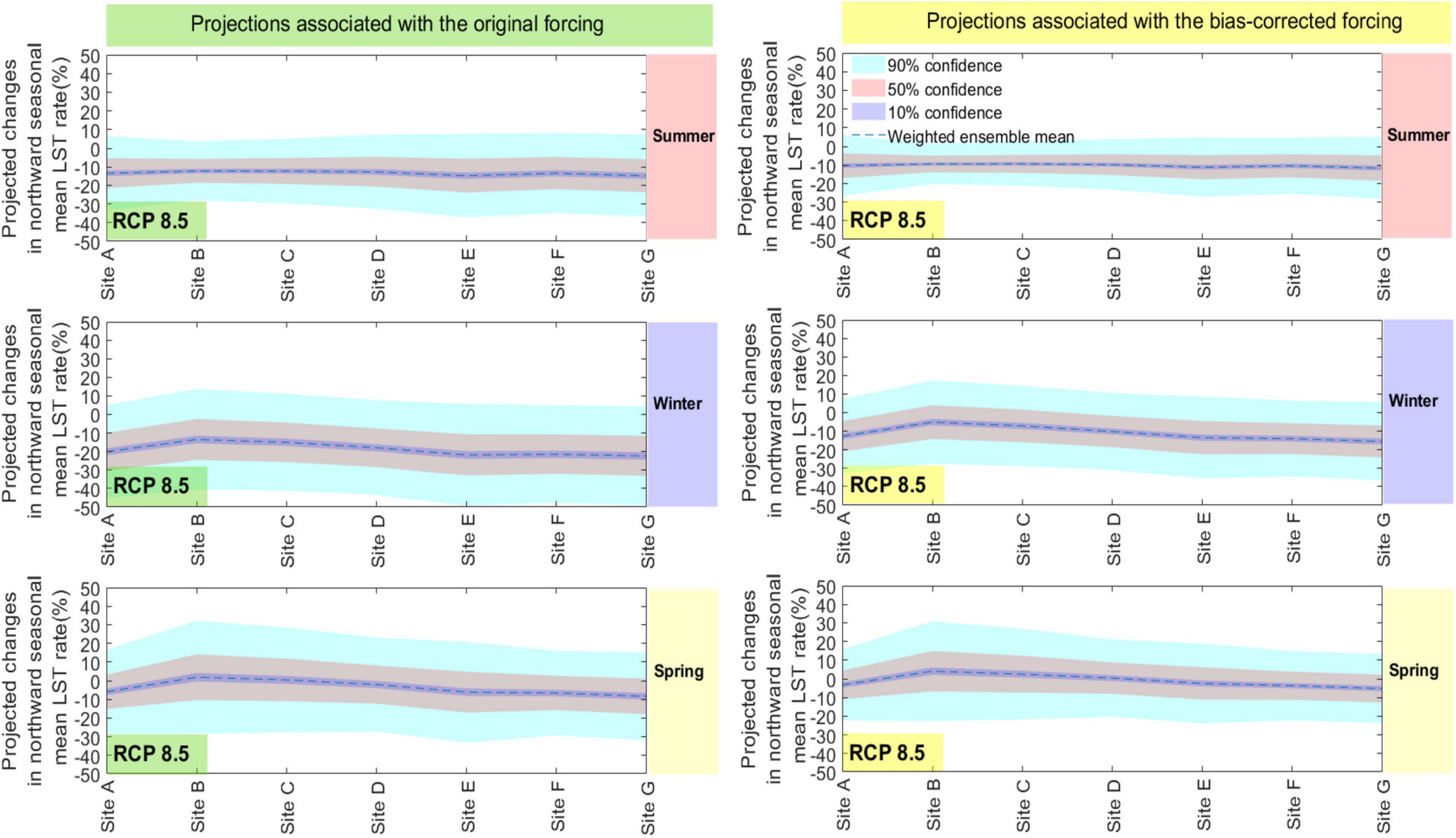
Figure 12. Projected changes in northward seasonal mean LST rates, under RCP 8.5, obtained from using the original forcing conditions (left panel) and the bias-corrected ones (rigth panel).
The robustness of the projected changes were checked by two straightforward approaches. In the first approach, for all sites, the ratio of signal to noise is less than one, showing that there is no robust projected changes in annul and seasonal mean LST rates. Using the second approach, less than 50% of the ensemble members showed a significant change in the LST rates. Hence, without any need to check the sign of the projected changes, it can be claimed that the projected changes are not robust (see Figure 13). Dealing with such results is challenging for coastal management systems as the ensemble mean of the projected changes is not reliable enough to enable the coastal planners to make future management decisions. For instance, if one relies on the ensemble mean of the projected changes, it might concluded that the operation of the sand bypassing system at site G, can be reduced by 10% to 20%. But in fact, the large variations in the projected changes degrade the reliability of any decision-making system working with the ensemble mean of the projected changes.
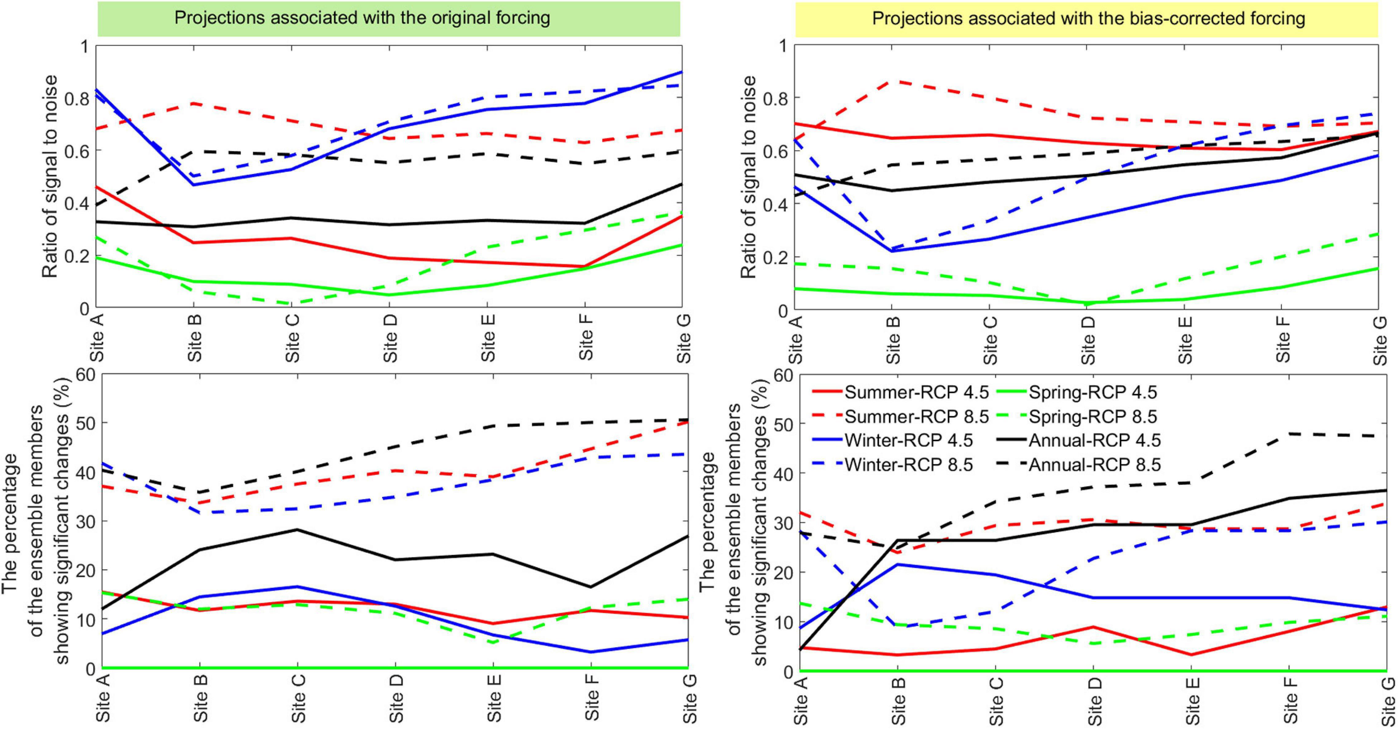
Figure 13. Robustness of the projected changes in LST rates along the coast on annual and seasonal scales associated with using original forcing conditions (left panel), and bias corrected forcing conditions (right panel); upper panel shows the ratio of signal to noise (first method for checking the robustness) and lower panel shows the percentage of the ensemble members showing significant changes (the second method for checking the robustness).
Limitations and the Way Forward
The computationally efficient LST models used in this study, could only be forced by the integral parameters of total wave energy. Currently, these models cannot directly work with wave energy spectrum or wave parameters of sea and swell partitions. Hence, integral parameters of total wave energy of the GCM-Ws datasets, were selected to reconstruct a single peak wave energy spectrum at the offshore boundary of the wave model, and the corresponding integral parameters of total wave energy at the nearshore region were given to the LST models. Regarding the representative wave direction for long-term morphodynamic studies, Dm which is influenced by both partitions of sea and swell (de Swart et al., 2020), was chosen. Although using the integral parameters of total wave energy at offshore region, has resulted in reasonable LST patterns for a historical period compared to the observations (e.g., Sedigh et al., 2016; Shaeri et al., 2019), still the range of uncertainty in LST projections might be different if a multiple-peak wave spectrum, (rather than a single-peak one) at the offshore region is used. Currently, there is a lack of an optimal method in literature to reconstruct the full shape of wave spectrum by using the integral parameters of sea and swell partitions (Albuquerque et al., 2021). In this regard, the shape of the spectrum for each partition should be assumed individually and the wave energy of the partitions should be superimposed, which itself might widen the range of uncertainty in the LST projections. Addressing this issue is a way forward to the current research. In addition, the effect of local wind on wave transformation was disregarded as the spatial resolutions of the GCMs (∼ one to three degrees) were not adequate to capture the patterns of local wind properly. In the near future, using new datasets of Coupled Model Intercomparison Project Phase 6 (CMIP6) with finer resolutions (e.g., Eyring et al., 2016), this source of uncertainty can be addressed. Moreover, by using more datasets of GCM-Ws (e.g., 50 datasets) with better temporal and spatial resolutions, a wider range of uncertainty for the projection of wave-driven sediment transport might be reported to coastal planners and decision makers.
The offshore wave climate of the study area is influenced by the large-scale climate system variability, acting on time scales of years to decades (Helman and Tomlinson, 2018). This natural variability can impact the trends of changes in offshore wave climate, and the resulting LST. Hence, having the time series of waves covering a long period for the baseline period and continuously projecting future wave climate (e.g., timeseries of waves for the time slice 1950–2100), is necessary to detect the contribution of natural variability (i.e., intrinsic uncertainty) to total uncertainty of the projected changes in coastal sediment transport patterns. Moreover, recent studies do not recommend using GCM-Ws directly for projection of future coastal evolution patterns (e.g., projection of shorelines), even in case of having continuous time series. Because the effect of natural variability of wave forcing on coastal evolution should also be addressed somehow (e.g., generating synthetic timeseries of waves; D’Anna et al., 2021). The timeseries of GCM-Ws used in this study, were neither continuous nor long enough to investigate these features of the climate change studies.
In this study, only a limited number of LST models, with constant settings for the baseline and future periods, were used to investigate the contribution of LST models to total uncertainty of the LST projections. However, setting up the sediment transport models, particularly the process-based ones, within probabilistic frameworks (Bamunawala et al., 2020, 2021) might result in an ensemble of the projections showing a greater contribution of sediment transport model uncertainty to total uncertainty (i.e., greater than 15%). This issue must be addressed in future studies.
Conclusion
Two ensembles for the projection of future patterns of LST were developed. The first one, consisted of eight datasets of GCM-Ws, projected under two emission scenarios, one hybrid wave transformation method, and eight LST models. The differentiating factor of the second ensemble was the application of bias correction to the GCM-Ws, given CAWCR 24 min as the reference forcing. The projected changes in LST obtained from each ensemble were introduced to ANOVA to find the contribution of RCPs, GCM-Ws, LST models, and their interactions, to total uncertainty of the LST projections. A simple scheme for weighting the ensembles’ members, and two approaches to check the robustness of the projections were also adopted. The results showed that application of bias correction relatively reduced the uncertainty of the projected changes in annual and seasonal LST patterns. In response to applying the bias correction to the forcing conditions, occasionally some meagre manipulation of the signals of climate change for the LST projections was observed. Applying ANOVA to the projected changes in annual LST rates, obtained from both ensembles, showed that the contribution of emission scenarios, GCM-Ws, LST models and their non-linear interactions to total uncertainty was about 10–20, 35–50, 5–15, and 30–35%, respectively. A large contribution of GCM-Ws together with the interaction of emission scenarios with GCM-Ws (overall greater than 60%) to total uncertainty of the LST projections, accentuates the relevance of using multiple wave climate projections (associated with different GCMS and emission scenarios) to better estimate the range of uncertainty. At the same time, this issue questions the reliability of any wave-driven sediment transport projections relying on a few GCM-Ws datasets under a single emission scenario. Using the weighted means of the ensembles, a decrease in net annual mean LST rates (less than 10% decrease under RCP 4.5, and a 10–20% decrease under RCP 8.5) was projected. However, after estimating the robustness of the projections, it was revealed that there are no robust projected changes in the LST rates, challenging any ultimate decision for coastal planning in terms of adaptation planning to climate change. In addition to the sources of uncertainties addressed in this study, the importance of accounting for the residual uncertainties (e.g., using GCMs with better spatial resolutions, inclusion of local wind in wave transformation, reconstructing the offshore boundary using the integral parameters of wind-sea and swell partitions, probabilistic simulation of the LST models) is emphasized.
Data Availability Statement
The original contributions presented in the study are included in the article/Supplementary Material, further inquiries can be directed to the corresponding author.
Author Contributions
AZ and JA: conceptualization, methodology, modelling and coding, and writing-review and editing. AE-S: conceptualization, methodology, writing-review and editing, funding acquisition, and supervision. NC and DS: conceptualization, methodology, and writing-review and editing. GL: coding and writing-review and editing. All authors contributed to the article and approved the submitted version.
Conflict of Interest
The authors declare that the research was conducted in the absence of any commercial or financial relationships that could be construed as a potential conflict of interest.
Publisher’s Note
All claims expressed in this article are solely those of the authors and do not necessarily represent those of their affiliated organizations, or those of the publisher, the editors and the reviewers. Any product that may be evaluated in this article, or claim that may be made by its manufacturer, is not guaranteed or endorsed by the publisher.
Acknowledgments
The authors would like to acknowledge the financial support from Griffith University. The authors also appreciate DHI for providing the license of the required models. The city of Gold Coast and the Queensland Government are much appreciated for providing the required data of this research, including bathymetries, hydrographic surveys, and wave-buoys data.
Supplementary Material
The Supplementary Material for this article can be found online at: https://www.frontiersin.org/articles/10.3389/fmars.2022.832193/full#supplementary-material
References
Adams, P. N., Inman, D. L., and Lovering, J. L. (2011). Effects of climate change and wave direction on longshore sediment transport patterns in Southern California. Clim. Change 109, 211–228. doi: 10.1007/s10584-011-0317-0
Albuquerque, J., Antolínez, J. A. A., Gorman, R. M., Méndez, F. J., and Coco, G. (2021). Seas and swells throughout New Zealand: a new partitioned hindcast. Ocean Model. 168:101897. doi: 10.1016/J.OCEMOD.2021.101897
Almar, R., Kestenare, E., Reyns, J., Jouanno, J., Anthony, E. J., Laibi, R., et al. (2015). Response of the bight of benin (Gulf of Guinea, West Africa) coastline to anthropogenic and natural forcing, Part1: wave climate variability and impacts on the longshore sediment transport. Cont. Shelf Res. 110, 48–59. doi: 10.1016/j.csr.2015.09.020
Alvarez-Cuesta, M., Toimil, A., and Losada, I. J. (2021). Modelling long-term shoreline evolution in highly anthropized coastal areas. Part 2: assessing the response to climate change. Coast. Eng. 168:103961. doi: 10.1016/J.COASTALENG.2021.103961
Amengual, A., Homar, V., Romero, R., Alonso, S., and Ramis, C. (2012). A statistical adjustment of regional climate model outputs to local scales: application to platja de palma. Spain. J. Clim. 25, 939–957. doi: 10.1175/JCLI-D-10-05024.1
Anderson, D., Ruggiero, P., Antolínez, J. A. A., Méndez, F. J., and Allan, J. (2018). A climate index optimized for longshore sediment transport reveals interannual and multidecadal littoral cell rotations. J. Geophys. Res. Earth Surf. 123, 1958–1981. doi: 10.1029/2018JF004689
Antolínez, J. A. A., Méndez, F. J., Anderson, D., Ruggiero, P., and Kaminsky, G. M. (2019). Predicting climate-driven coastlines with a simple and efficient multiscale model. J. Geophys. Res. Earth Surf. 124, 1596–1624. doi: 10.1029/2018JF004790
Antolínez, J. A. A., Méndez, F. J., Camus, P., Vitousek, S., González, E. M., Ruggiero, P., et al. (2016). A multiscale climate emulator for long-term morphodynamics (MUSCLE-morpho). J. Geophys. Res. Ocean 121, 775–791. doi: 10.1002/2015JC011107
Antolínez, J. A. A., Murray, A. B., Méndez, F. J., Moore, L. J., Farley, G., and Wood, J. (2018). Downscaling changing coastlines in a changing climate: the hybrid approach. J. Geophys. Res. Earth Surf. 123, 229–251. doi: 10.1002/2017JF004367
Bamunawala, J., Dastgheib, A., Ranasinghe, R., van der Spek, A., Maskey, S., Murray, A. B., et al. (2020). Probabilistic application of an integrated catchment-estuary-coastal system model to assess the evolution of inlet-interrupted coasts over the 21st century. Front. Mar. Sci. 7:1104. doi: 10.3389/FMARS.2020.579203/BIBTEX
Bamunawala, J., van der Spek, A., Dastgheib, A., Murray, A. B., and Ranasinghe, R. (2021). An integrated, probabilistic modeling approach to assess the evolution of barrier-island systems over the twenty-first century. Front. Mar. Sci. 8:1708. doi: 10.3389/FMARS.2021.755699/BIBTEX
Başaran, B., and Arı Güner, H. A. (2021). Effect of wave climate change on longshore sediment transport in Southwestern Black Sea. Estuar. Coast. Shelf Sci. 258:107415. doi: 10.1016/J.ECSS.2021.107415
Bonaldo, D., Benetazzo, A., Sclavo, M., and Carniel, S. (2015). Modelling wave-driven sediment transport in a changing climate: a case study for northern Adriatic Sea (Italy). Reg. Environ. Chang. 15, 45–55. doi: 10.1007/s10113-014-0619-7
Bosshard, T., Carambia, M., Goergen, K., Kotlarski, S., Krahe, P., Zappa, M., et al. (2013). Quantifying uncertainty sources in an ensemble of hydrological climate-impact projections. Water Resour. Res. 49, 1523–1536. doi: 10.1029/2011WR011533
Brands, S., Herrera, S., San-Martín, D., and Gutierrez, J. M. (2011). Validation of the ENSEMBLES global climate models over southwestern Europe using probability density functions, from a downscaling perspective. Clim. Res. 48, 145–161. doi: 10.3354/CR00995
Cagigal, L., Rueda, A., Anderson, D., Ruggiero, P., Merrifield, M. A., Montaño, J., et al. (2020). A multivariate, stochastic, climate-based wave emulator for shoreline change modelling. Ocean Model. 154:101695. doi: 10.1016/j.ocemod.2020.101695
Camus, P., Losada, I. J., Izaguirre, C., Espejo, A., Menéndez, M., and Pérez, J. (2017). Statistical wave climate projections for coastal impact assessments. Earth’s Fut. 5, 918–933. doi: 10.1002/2017EF000609
Camus, P., Mendez, F. J., and Medina, R. (2011). A hybrid efficient method to downscale wave climate to coastal areas. Coast. Eng. 58, 851–862. doi: 10.1016/j.coastaleng.2011.05.007
Casas-Prat, M., McInnes, K. L., Hemer, M. A., and Sierra, J. P. (2016). Future wave-driven coastal sediment transport along the Catalan coast (NW Mediterranean). Reg. Environ. Chang. 16, 1739–1750. doi: 10.1007/s10113-015-0923-x
Chowdhury, P., Behera, M. R., and Reeve, D. E. (2020). Future wave-climate driven longshore sediment transport along the Indian coast. Clim. Change 162, 405–424. doi: 10.1007/s10584-020-02693-7
D’Anna, M., Castelle, B., Idier, D., Rohmer, J., Le Cozannet, G., Thieblemont, R., et al. (2021). Uncertainties in shoreline projections to 2100 at truc vert beach (France): role of sea-level rise and equilibrium model assumptions. J. Geophys. Res. Earth Surf. 126:e2021JF006160. doi: 10.1029/2021JF006160
Dastgheib, A., Reyns, J., Thammasittirong, S., Weesakul, S., Thatcher, M., and Ranasinghe, R. (2016). Variations in the wave climate and sediment transport due to climate change along the coast of Vietnam. J. Mar. Sci. Eng. 4:86. doi: 10.3390/jmse4040086
de Queiroz, B., Scheel, F., Caires, S., Walstra, D. J., Olij, D., Yoo, J., et al. (2019). Performance evaluation of wave input reduction techniques for modeling inter-annual sandbar dynamics. J. Mar. Sci. Eng. 7:148. doi: 10.3390/jmse7050148
de Swart, R. L., Ribas, F., Calvete, D., Kroon, A., and Orfila, A. (2020). Optimal estimations of directional wave conditions for nearshore field studies. Cont. Shelf Res. 196:104071. doi: 10.1016/j.csr.2020.104071
DHL (1992). Southern Gold Coast Littoral Sand Supply. Technical Report H85, Delft Hydraulics Laboratory.
Eyring, V., Bony, S., Meehl, G. A., Senior, C. A., Stevens, B., Stouffer, R. J., et al. (2016). Overview of the coupled model intercomparison project phase 6 (CMIP6) experimental design and organization. Geosci. Model Dev. 9, 1937–1958. doi: 10.5194/GMD-9-1937-2016
GCCM (2017). Seaway Evolution – Morphological Trends and Processes – GCWA SRMP-006. Gold Coast, QLD: Griffith Centre for Coastal Management (Coastal and Marine Research Centre – CMRC).
Hanley, M. E., Hoggart, S. P. G., Simmonds, D. J., Bichot, A., Colangelo, M. A., Bozzeda, F., et al. (2014). Shifting sands? Coastal protection by sand banks, beaches and dunes. Coast. Eng. 87, 136–146. doi: 10.1016/j.coastaleng.2013.10.020
Hawkins, E., and Sutton, R. (2009). The potential to narrow uncertainty in regional climate predictions. Bull. Am. Meteorol. Soc. 90, 1095–1107. doi: 10.1175/2009BAMS2607.1
Hay, L. E., Wilby, R. L., and Leavesley, G. H. (2000). A comparison of delta change and downscaled gcm scenarios for three mountainous basins in the united states1. JAWRA J. Am. Water Resour. Assoc. 36, 387–397. doi: 10.1111/J.1752-1688.2000.TB04276.X
Helman, P., and Tomlinson, R. (2018). Two centuries of climate change and climate variability, East Coast Australia. J. Mar. Sci. Eng. 6:3. doi: 10.3390/jmse6010003
Hemer, M. A., and Trenham, C. E. (2016). Evaluation of a CMIP5 derived dynamical global wind wave climate model ensemble. Ocean Model. 103, 190–203. doi: 10.1016/j.ocemod.2015.10.009
Hersbach, H., Bell, B., Berrisford, P., Hirahara, S., Horányi, A., Muñoz-Sabater, J., et al. (2020). The ERA5 global reanalysis. Q. J. R. Meteorol. Soc. 146, 1999–2049. doi: 10.1002/qj.3803
IPCC (2014). “Coastal systems and low-lying areas,” in Climate Change 2014 Impacts, Adaptation, and Vulnerability, eds C. B. Field, V. R. Barros, D. J. Dokken, K. J. Mach, and M. D. Mastrandrea (Cambridge: Cambridge University Press), 361–410. doi: 10.1017/CBO9781107415379.010
Jones, B., O’Neill, B. C., Jones, B., and O’Neill, B. C. (2016). Spatially explicit global population scenarios consistent with the shared socioeconomic pathways. ERL 11:084003. doi: 10.1088/1748-9326/11/8/084003
Kristensen, S. E., Drønen, N., Deigaard, R., and Fredsoe, J. (2016). Impact of groyne fields on the littoral drift: a hybrid morphological modelling study. Coast. Eng. 111, 13–22. doi: 10.1016/J.COASTALENG.2016.01.009
Le Cozannet, G., Oliveros, C., Castelle, B., Garcin, M., Idier, D., Pedreros, R., et al. (2016). Uncertainties in sandy shorelines evolution under the bruun rule assumption. Front. Mar. Sci. 3:49. doi: 10.3389/fmars.2016.00049
Lemos, G., Menendez, M., Semedo, A., Camus, P., Hemer, M., Dobrynin, M., et al. (2020a). On the need of bias correction methods for wave climate projections. Glob. Planet. Change 186:103109. doi: 10.1016/j.gloplacha.2019.103109
Lemos, G., Menendez, M., Semedo, A., Miranda, P. M. A., and Hemer, M. (2021a). On the decreases in North Atlantic significant wave heights from climate projections. Clim. Dyn. 2021, 1–24. doi: 10.1007/S00382-021-05807-8
Lemos, G., Semedo, A., Dobrynin, M., Behrens, A., Staneva, J., Bidlot, J.-R., et al. (2019). Mid-twenty-first century global wave climate projections: results from a dynamic CMIP5 based ensemble. Glob. Planet. Change 172, 69–87. doi: 10.1016/j.gloplacha.2018.09.011
Lemos, G., Semedo, A., Dobrynin, M., Menendez, M., and Miranda, P. M. A. (2020b). Bias-corrected CMIP5-derived single-forcing future wind-wave climate projections toward the end of the twenty-first century. J. Appl. Meteorol. Climatol. 59, 1393–1414. doi: 10.1175/JAMC-D-19-0297.1
Lemos, G., Semedo, A., Hemer, M., Menendez, M., and Miranda, P. M. A. (2021b). Remote climate change propagation across the oceans—the directional swell signature. Environ. Res. Lett. 16, 064080. doi: 10.1088/1748-9326/ac046b
Maraun, D. (2016). Bias correcting climate change simulations - a critical review. Curr. Clim. Chang. Rep. 2, 211–220. doi: 10.1007/s40641-016-0050-x
Mathews, R. J., Stutz, M. L., and Smith, A. W. S. (1998). A field investigation study to determine the properties of windblown beach sand. J. Coast. Res. 14, 444–450.
Meucci, A., Young, I. R., Hemer, M., Kirezci, E., and Ranasinghe, R. (2020). Projected 21st century changes in extreme wind-wave events. Sci. Adv. 6:eaaz7295. doi: 10.1126/sciadv.aaz7295
Mil-Homens, J., Ranasinghe, R., van Thiel de Vries, J. S. M., and Stive, M. J. F. (2013). Re-evaluation and improvement of three commonly used bulk longshore sediment transport formulas. Coast. Eng. 75, 29–39. doi: 10.1016/j.coastaleng.2013.01.004
Morim, J., Hemer, M., Cartwright, N., Strauss, D., and Andutta, F. (2018). On the concordance of 21st century wind-wave climate projections. Glob. Planet. Change 167, 160–171. doi: 10.1016/j.gloplacha.2018.05.005
Morim, J., Trenham, C., Hemer, M., Wang, X. L., Mori, N., Casas-Prat, M., et al. (2020). A global ensemble of ocean wave climate projections from CMIP5-driven models. Sci. Data 7, 1–10. doi: 10.1038/s41597-020-0446-2
O’Grady, J., Babanin, A., and McInnes, K. (2019). Downscaling future longshore sediment transport in South Eastern Australia. J. Mar. Sci. Eng. 7:289. doi: 10.3390/jmse7090289
Ranasinghe, R. (2016). Assessing climate change impacts on open sandy coasts: a review. Earth-Science Rev. 160, 320–332. doi: 10.1016/j.earscirev.2016.07.011
Ranji, Z., Zarifsanayei, A. R., Cartwright, N., and Soltanpour, M. (2022). Climate change impacts on tropical cyclones of the Arabian Sea: projections and uncertainty investigations. Int. J. Climatol. doi: 10.1002/joc.7523
Roelvink, D., Huisman, B., Elghandour, A., Ghonim, M., and Reyns, J. (2020). Efficient modeling of complex sandy coastal evolution at monthly to century time scales. Front. Mar. Sci. 7:535. doi: 10.3389/fmars.2020.00535
Ruggiero, P., Buijsman, M., Kaminsky, G. M., and Gelfenbaum, G. (2010). Modeling the effects of wave climate and sediment supply variability on large-scale shoreline change. Mar. Geol. 273, 127–140. doi: 10.1016/j.margeo.2010.02.008
Sanderson, B. M., Knutti, R., and Caldwell, P. (2015). A representative democracy to reduce interdependency in a multimodel ensemble. J. Clim. 28, 5171–5194. doi: 10.1175/JCLI-D-14-00362.1
Sedigh, M., Tomlinson, R., Cartwright, N., and Etemad-Shahidi, A. (2016). Numerical modelling of the Gold Coast Seaway area hydrodynamics and littoral drift. Ocean Eng. 121, 47–61. doi: 10.1016/j.oceaneng.2016.05.002
Shaeri, S., Etemad-Shahidi, A., Strauss, D., and Tomlinson, R. (2019). Accelerated numerical simulation to investigate morphology changes around small tidal inlets. Coast. Eng. J. 61, 535–558. doi: 10.1080/21664250.2019.1651562
Shaeri, S., Etemad-Shahidi, A., and Tomlinson, R. (2020). Revisiting longshore sediment transport formulas. J. Waterw. Port Coast. Ocean Eng. 146:04020009. doi: 10.1061/(ASCE)WW.1943-5460.0000557
Smith, G. A., Hemer, M., Greenslade, D., Trenham, C., Zieger, S., and Durrant, T. (2020). Global wave hindcast with Australian and Pacific Island focus: from past to present. Geosci. Data J. 8, 24–33. doi: 10.1002/gdj3.104
Splinter, K. D., and Coco, G. (2021). Challenges and opportunities in coastal shoreline prediction. Front. Mar. Sci. 0:1917. doi: 10.3389/FMARS.2021.788657
Splinter, K. D., Davidson, M. A., Golshani, A., and Tomlinson, R. (2012). Climate controls on longshore sediment transport. Cont. Shelf Res. 48, 146–156. doi: 10.1016/j.csr.2012.07.018
Tebaldi, C., Arblaster, J. M., and Knutti, R. (2011). Mapping model agreement on future climate projections. Geophys. Res. Lett. 38, 1–5. doi: 10.1029/2011GL049863
Toimil, A., Camus, P., Losada, I. J., and Alvarez-Cuesta, M. (2021). Visualising the uncertainty cascade in multi-ensemble probabilistic coastal erosion projections. Front. Mar. Sci. 8:679. doi: 10.3389/FMARS.2021.683535
Toimil, A., Camus, P., Losada, I. J., Le Cozannet, G., Nicholls, R. J., Idier, D., et al. (2020). Climate change-driven coastal erosion modelling in temperate sandy beaches: methods and uncertainty treatment. Earth-Science Rev. 202:103110. doi: 10.1016/j.earscirev.2020.103110
van Rijn, L. C. (2014). A simple general expression for longshore transport of sand, gravel and shingle. Coast. Eng. 90, 23–39. doi: 10.1016/j.coastaleng.2014.04.008
Vieira Da Silva, G., Murray, T., and Strauss, D. (2018). Longshore wave variability along non-straight coastlines. Estuar. Coast. Shelf Sci. 212, 318–328. doi: 10.1016/j.ecss.2018.07.022
Vitousek, S., Barnard, P. L., Limber, P., Erikson, L., and Cole, B. (2017). A model integrating longshore and cross-shore processes for predicting long-term shoreline response to climate change. J. Geophys. Res. Earth Surf. 122, 782–806. doi: 10.1002/2016JF004065
Vitousek, S., Cagigal, L., Montaño, J., Rueda, A., Mendez, F., Coco, G., et al. (2021). The application of ensemble wave forcing to quantify uncertainty of shoreline change predictions. J. Geophys. Res. Earth Surf 126:e2019JF005506. doi: 10.1029/2019JF005506
Wang, F., Huang, G. H., Fan, Y., and Li, Y. P. (2020). Robust subsampling ANOVA methods for sensitivity analysis of water resource and environmental models. Water Resour. Manag. 34, 3199–3217. doi: 10.1007/S11269-020-02608-2
Yip, S., Ferro, C. A. T., Stephenson, D. B., and Hawkins, E. (2011). A simple, coherent framework for partitioning uncertainty in climate predictions. J. Clim. 24, 4634–4643. doi: 10.1175/2011JCLI4085.1
Zacharioudaki, A., and Reeve, D. E. (2011). Shoreline evolution under climate change wave scenarios. Clim. Change 108, 73–105. doi: 10.1007/s10584-010-0011-7
Zarifsanayei, A. R., Antolínez, J. A. A., Etemad-Shahidi, A., Cartwright, N., and Strauss, D. (2022). A multi-model ensemble to investigate uncertainty in the estimation of wave-driven longshore sediment transport patterns along a non-straight coastline. Coast. Eng. 173:04080. doi: 10.1016/j.coastaleng.2022.104080
Zarifsanayei, A. R., Etemad-Shahidi, A., Cartwright, N., and Strauss, D. (2020). Long-term prediction of longshore sediment transport in the context of climate change. Coast. Eng. Proc. 36. Available online at: https://doi.org/10.9753/icce.v36v.papers.15 (accessed December 31, 2020).
Keywords: uncertainty, longshore sediment transport, ensemble modelling, climate change, projection of wave-driven sediment transport patterns, robustness of projections
Citation: Zarifsanayei AR, Antolínez JAA, Etemad-Shahidi A, Cartwright N, Strauss D and Lemos G (2022) Uncertainties in the Projected Patterns of Wave-Driven Longshore Sediment Transport Along a Non-straight Coastline. Front. Mar. Sci. 9:832193. doi: 10.3389/fmars.2022.832193
Received: 09 December 2021; Accepted: 25 January 2022;
Published: 28 February 2022.
Edited by:
Juan Jose Munoz-Perez, University of Cádiz, SpainReviewed by:
Giuseppe Barbaro, Mediterranea University of Reggio Calabria, ItalyJulian O’Grady, Climate Science Centre, Commonwealth Scientific and Industrial Research Organization, Australia
Copyright © 2022 Zarifsanayei, Antolínez, Etemad-Shahidi, Cartwright, Strauss and Lemos. This is an open-access article distributed under the terms of the Creative Commons Attribution License (CC BY). The use, distribution or reproduction in other forums is permitted, provided the original author(s) and the copyright owner(s) are credited and that the original publication in this journal is cited, in accordance with accepted academic practice. No use, distribution or reproduction is permitted which does not comply with these terms.
*Correspondence: José A. A. Antolínez, J.A.A.Antolinez@tudelft.nl