Oceanic response to typhoons in the Northwest Pacific using Aquarius and SMAP data (2011–2020)

1. Introduction

Typhoons, as mature tropical cyclones, are one of the most devastating oceanic and atmospheric phenomena that occur through intense air-sea interactions (Price, 1981). They cause destructive damage to vulnerable coastal regions. However, they also play an important role in maintaining the thermal balance of unequal heat exchange between tropical and subtropical regions (Emanuel, 2001; Medvedev et al., 2022). Strong sea surface winds change the depth of the oceanic mixed layer owing to vigorous turbulent mixing, leading to cooling of the sea surface and upper ocean temperature, which is related to the intensity of the typhoon through a feedback mechanism (Fedorov, 1979; Price, 1981; Price, 1983; Emanuel, 1991). Another positive aspect of typhoons is that changes in the physical and biogeochemical environment, such as vigorous turbulent mixing and upwelling of nutrient supply, enhance bioactivity during and after the typhoon passage (Mooers, 1975; Siswanto et al., 2009; Chen et al., 2021; Topor et al., 2022). With regards to the response of sea surface temperature (SST) to the typhoons, studies have demonstrated that surface cooling induced by the turbulent mixing with emphasized responses is more dominant on the right side of the typhoons (Cornillon et al., 1987; Emanuel, 2001; D'Asaro et al., 2007; Glenn et al., 2016). Surface cooling has been well demonstrated by infrared and microwave remote sensing satellites.

Similar to the SST, sea surface salinity (SSS) is one of the most important variables affecting oceanic circulation and global hydrological cycle (Klemas, 2011). It plays a fundamental role in controlling and regulating recent climate change (Cooper, 1988; Lagerloef, 2008) and can act as a signal for water exchange between the ocean and atmosphere through the processes of evaporation and precipitation on regional and global scales (Curry et al., 2003). Moreover, it is strongly correlated with freshwater input and output to the ocean through diverse processes, such as evaporation, precipitation, melting and formation of sea ice, and river discharge (Lagerloef, 2002; Durack et al., 2012). During the typhoon events, strong winds cause a positive salinity flux from the sea surface to the atmosphere due to the violent evaporation of salt. However, the SSS decreases because of the effects of intensive rainfall within the passage of typhoon (Bond et al., 2011; Girishkumar et al., 2014; Liu et al., 2020). Precipitation causes a negative SSS anomaly on the left side of the typhoon track in the Northern Hemisphere (Grodsky et al., 2012). Continuous and repetitive satellite SSS observations can monitor the spatial and temporal changes in the ocean salinity during the typhoons.

The successful launch and operation of Soil Moisture and Ocean Salinity (SMOS), Aquarius, and Soil Moisture Active Passive (SMAP) satellites have enabled the observation of the spatial distribution of the SSS from in situ salinity measurements (Lagerloef et al., 1995; Bingham et al., 2002; Reul et al., 2012). Various instruments, such as conductivity, temperature, and depth measurements by moored buoys, ship observations, and Argo floats, provided high-quality salinity data prior to the operation of these satellites. However, most in situ data on the ocean salinity was limited to reproducing the spatial distribution of SSS in the global ocean and local seas. With the launch of the SMOS, Aquarius/SAC-D, and SMAP satellites on November 2009, June 2011, and January 2015, respectively, the distribution of the SSS can be observed over a wide area of the ocean in real time (Font et al., 2004; LeVine et al., 2007; Tranchant et al., 2008; Yueh et al., 2013).

Many studies have investigated the accuracy of the SSS in the global ocean and regional seas (Boutin et al., 2013; Abe and Ebuchi, 2014; Drucker and Riser, 2014; Kim et al., 2014; Menezes et al., 2014; Ratheesh et al., 2014; Tang et al., 2014; Bhaskar and Jayaram, 2015; D'Addezio and Subrahmanyam, 2016a; D'Addezio and Subrahmanyam, 2016b; Fournier et al., 2016; Tzortzi et al., 2016; Tang et al., 2017; Bao et al., 2019). Its accuracy is 0.2 psu for a monthly average within 1°×1° or in a spatial resolution of 150 km (Lagerloef, 2008; Lagerloef and Font, 2010). In addition, compared to the in situ measurements, the satellite SSS data have shown root mean square error (RMSE) of less than 0.5 psu in the global ocean, such as 0.42 psu (Abe and Ebuchi, 2014; Drucker and Riser, 2014), 0.31 psu (Reagan et al., 2014), 0.495 psu (Tang et al., 2014), 0.45 psu (Ratheesh et al., 2014), 0.21 psu (SMOS), and 0.23 psu (SMAP) (Bao et al., 2019). Larger SSS errors were found in the regions; high-latitude region, the Atlantic Ocean near the Amazon River with considerable river input, intertropical convergence zones, particularly the Eastern Pacific Fresh Pool and the South Pacific Convergence Zone (Tang et al., 2014). Some studies have identified the differences in measurement depth between the satellites within 2–3 cm from the sea surface and top Argo float measurements at depths of 1–7 m as the potential sources of these errors (Drucker and Riser, 2014). Such differences can create errors greater than −0.1 psu when changes in the vertical stability of the upper surface layer are induced by precipitation (Drucker and Riser, 2014).

It is important to investigate which oceanic conditions and geolocations are pertinent in order to use the satellite salinity data in the typhoon studies. Figure 1A shows the spatial distribution of the SMAP SSSs in the global ocean averaged over 4 years from April 2015 to December 2020. The overall features as well as the SSS values of SMAP are quite similar to the annual mean of the World Ocean Atlas (WOA) 2018 SSSs during the period from 2005 to 2017 (Figure 1B). The SSS differences between SMAP and WOA have magnitudes of approximately 1.0 psu in the global ocean (Figure 1C). In the Northwest Pacific, there are differences of approximately 0.5−1.0 psu. To investigate whether the satellite SSSs can be used for the typhoon studies, we conducted a validation of the satellite salinity in the northwest Pacific Ocean, as illustrated in Figure 1D, and examined the oceanic responses of the upper ocean to the typhoons.

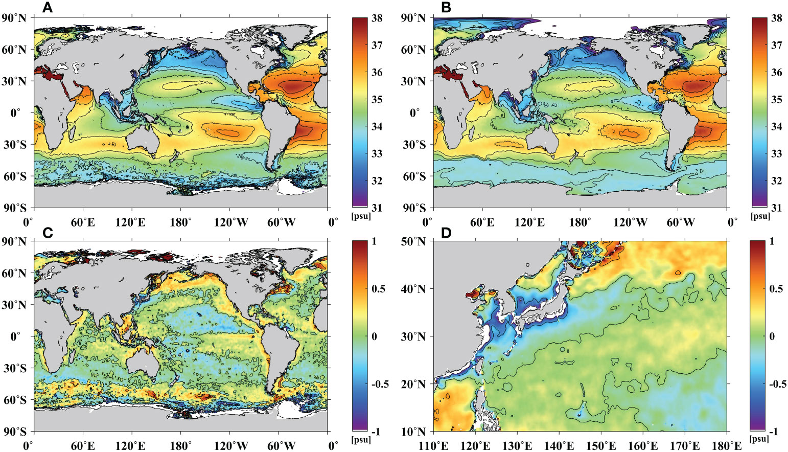
Figure 1 Spatial distributions of (A) Soil Moisture Active Passive (SMAP) satellite sea surface salinity (SSS) averaged over the period of 2015 to 2020, (B) mean SSS from World Ocean Atlas (WOA) 2018 over the period of 2005–2017, (C) differences between the SMAP and WOA salinity in the global ocean, and (D) enlarged portion of salinity differences in the Northwest Pacific from (C).

It has recently been observed that the SSS drops amplify after passing through the tropical storms to the left of the track in the case of slow-moving storms (Reul et al., 2021). However, two-dimensional (2-D) features of oceanic salinity responses to the typhoon forcings as well as other atmospheric and oceanic variables have not been presented, especially along the tracks of the typhoons. The spatial distribution of the salinity responses is critical for understanding the air-sea interactions during the typhoon passage. Therefore, the objectives of this study were: (1) to assess the accuracy of the satellite SSS compared to the in situ salinity measurements in the Northwest Pacific Ocean, (2) to examine the characteristics of the SSS errors and investigate whether the satellite SSSs can be used for the study of typhoons, (3) to examine the upper ocean response in the Northwest Pacific during typhoon events, and (4) to investigate the potential cause of the oceanic salinity change by following the typhoon paths.

2. Data and methods

2.1. Satellite data

We estimated the accuracies of the SSS of Aquarius and SMAP and examined the characteristics of the errors to investigate the applicability of satellite-observed SSS for studying the sea surface response during the typhoon period. For Aquarius, level-2 version 5.0 SSS data with a resolution of 100 km × 100 km from the National Aeronautics and Space Administration (NASA) Jet Propulsion Laboratory from the period January 2012 to December 2014 were used (Kao et al., 2018; Le Vine et al., 2018; Meissner et al., 2018). In addition, level-2 version-5 SMAP SSS data products of NASA from April 2015 to August 2020 were used. Quality flags of the SSS measurements were applied to remove the data contamination factors, such as ice, rainfall, and landmass (Santos-Garcia et al., 2014; Tang et al., 2014). Microwave AMSR-2 data, such as sea surface temperature, wind speed, precipitation, and water vapor data, were obtained from Remote Sensing Systems (www.remss.com) (Wentz et al., 2014).

2.2. Argo data

Argo data from the Argo Data Center and Global Data Assembly Center are widely utilized for diverse purposes (ftp://ftp.ifremer.fr/ifremer/argo). We collocated the SSS data at the depth nearest to the sea surface for comparison with the SSS data. Quality-controlled Argo data passing through real-time and delayed mode processing (Wong et al., 2003) were used to assess the accuracy of the satellite salinity and investigate the oceanic response during the typhoon events. Argo vertical profile temperature and salinity data of the upper ocean were used to examine the changes in temperature and salinity after the typhoon passage.

2.3. In situ salinity measurement data

To validate the satellite-derived surface salinity, salinity data from the World Ocean Database 2013 with a full set of quality controls were obtained from the National Oceanographic Data Center (Conkright et al., 2002; Garcia et al., 2010). The temperature and salinity profiles of the Argo float at a depth near the sea surface (3–5 m) were analyzed to investigate the upper ocean response during the typhoon period. The annual mean salinity of the WOA 2018 with a spatial resolution of 0.25° × 0.25° from 2005 to 2017 was also used for the overall comparison of salinity distribution.

2.4. Matchup procedure

Satellite SSSs at temperatures of less than 5°C are relatively inaccurate because of the low sensitivity of the L-band sensor to surface radiance (Yueh et al., 2001; Abe and Ebuchi, 2014). Therefore, we eliminated the SSSs observed in regions with low SSTs (<5°C) prior to the estimation of its accuracy. A quality control process was applied to exclude the SSS values under poor atmospheric and oceanic conditions (Abe and Ebuchi, 2014). In addition, pixels with a large fraction of land (>0.0005) near the coast were removed from the satellite SSS values to maintain good quality in the matchup procedure, considering land contamination in the coastal region (Reul et al., 2012; Abe and Ebuchi, 2014).

Each individual satellite salinity value was collocated with the in situ observations of the Argo data within a 12 h temporal interval. The spatial window of the matchup procedure was within a distance of 100 km and 40 km for the Aquarius and SMAP SSS, respectively. The matchup database was composed of the satellite SSS, in situ salinity, temporal information, geolocation information, and depths of the in situ salinity. Other auxiliary data, such as wind speed, SST, and rain rate, were also obtained from collocations among the satellite SSSs, in situ measurements, and passive microwave sensor data. In addition, the distance of each matchup point from the nearest coast was calculated to examine the potential effects of the coastal region.

2.5. Typhoon data

Information on typhoons over the Northwest Pacific Ocean from the Aquarius and SMAP satellites from 2012 to 2020 was obtained from Korea Meteorological Agency (KMA) Open Met Data Portal (https://data.kma.go.kr/data/typhoonData/typList.do?pgmNo=688). A graphical representation of the typhoon tracks is shown using colored lines in Figure 2. The typhoon information of KMA revealed that 240 typhoons occurred in the Northwest Pacific during the study period. We applied a few criteria on the characteristics of the typhoons to select the appropriate tracks for the response of the upper ocean salinity. In particular, typhoons that deviated from the study area (120–180°E, 10–50°N) and occurred from December to June were excluded. Typhoons with parabolic paths open to the east were selected by avoiding typhoons moving westward and landing on land with a relatively short path over the ocean. To select typhoons with a smooth parabolic curve, we least-square fitted optimally the latitude Y (°N) and longitude X (°E) values of the typhoon trajectory to the following Equation (1) and derived coefficients (a₁, a₂, and a₃).

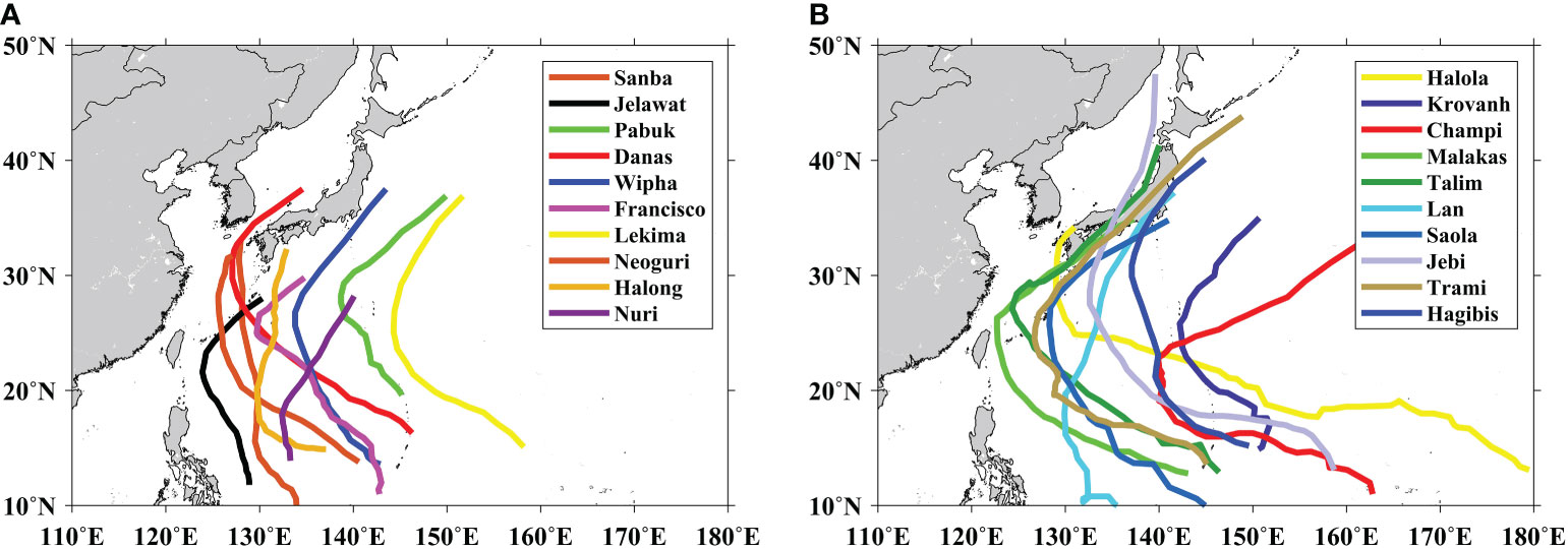
Figure 2 Spatial distribution of the representative typhoon passage tracks used in this study for (A) Aquarius (2011–2015) and (B) Soil Moisture Active Passive (SMAP) (2015–2020) in the Northwest Pacific.

Typhoons with a negative or weakly positive coefficient (a₁< 0.0173) were eliminated. In addition, we examined the locations of the inflection points of the typhoon paths, giving a range of 120-145°E. The inflection points of all typhoons that satisfied the limit of coefficient a₁ were located in the west. The mean longitude of the 20 inflection points was approximately 130.6°E. Finally, 20 typhoons satisfied these conditions. Table 1 summarizes the characteristics of the typhoons used for the study of salinity responses. The mean radius with maximum radius above 15 m s^-1 of the 20 typhoons was approximately 312 km. Most of the typhoons with small radius (<300 km) were automatically removed through the parabolic test. Typhoons passing within (<200 km) of the coastal region in low-latitude regions between 10°N and 30°N were eliminated through the above test.

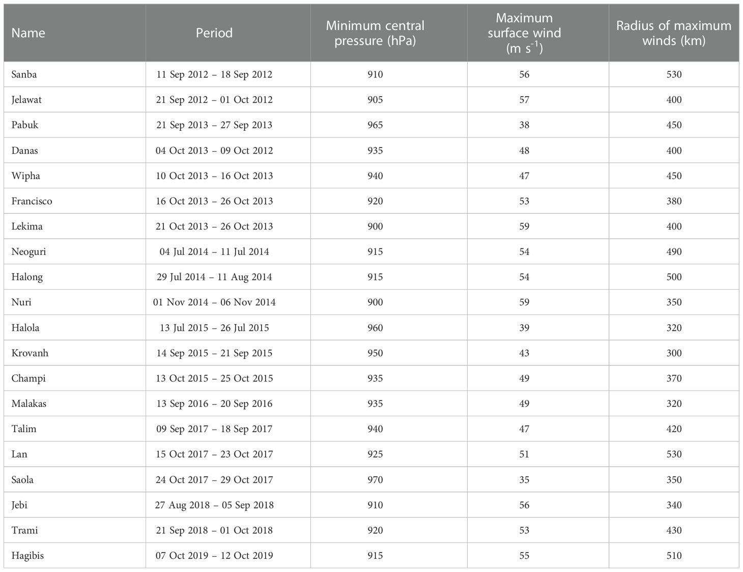
Table 1 Information of the typhoons used in this study in the Northwest Pacific from Aquarius and Soil Moisture Active Passive (SMAP) satellites during 2011 to 2020.

It is hypothesized that the SSS signal would be relatively high over regions with a large amount of precipitation. Considering this hypothesis, we eliminated relatively weak typhoons with high central pressures (>975 hPa) and low wind speeds (<35 m s^-1) at their peak values during the lifetime of each typhoon. Ultimately, 10 typhoons remained for Aquarius after passing the rejection criteria, including Sanba, Jelawat, Pabuk, Danas, Wipha, Francisco, Lekima, Neoguri, Halong, and Nuri, during 2012–2015 as shown in Table 1 and Figure 2A. In the case of SMAP, additional 10 typhoons, such as Halola, Krovanh, Champi, Malakas, Talim, Lan, Saola, Jebi, Trami, and Hagibis, from 2015–2019 remained after passing the rejection criteria (Table 1). To investigate the occurrence of oceanic responses, we set a time limit of up to 10 days before and after the arrival of each typhoon. Details of the 20 typhoons (period, minimum central pressure, maximum surface wind speed, and radius of maximum wind speed) used in this study are shown in Table 1. The oceanic and atmospheric responses to the typhoons were investigated by transforming the coordinate system in the typhoon path direction.

3. Results

3.1. Accuracy of satellite SSS in the Northwest Pacific

To understand the gross errors and uncertainties of the satellite-derived SSS in the Northwest Pacific, we estimated the accuracies of the Aquarius and SMAP SSS data by comparing with the collocated in situ salinity measurements, including the Argo data. Table 2 shows the number of collocated data and accuracies of the satellite SSSs. The number of collocation points of Aquarius and SMAP were 6,279 from January 2012 to December 2014 and 70,120 from April 2015 to August 2020 in the Northwest Pacific.

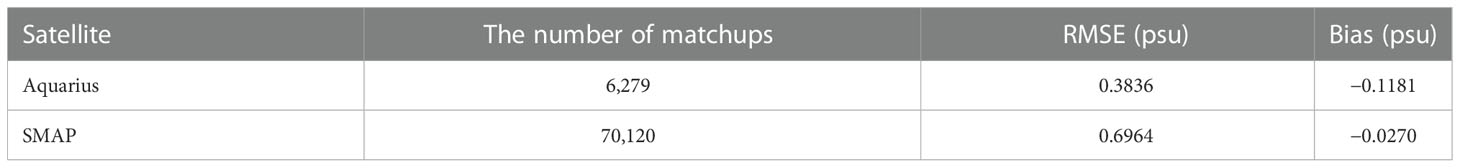
Table 2 Accuracies of satellite-observed sea surface salinity in the Northwest Pacific for Aquarius (2011–2015) and Soil Moisture Active Passive (SMAP) (2015–2020) by using matchup data with salinity data from Argo floats.

Figure 3 illustrates the time variations in the latitudinal SSS accuracies of the Aquarius and SMAP satellites with respect to the Argo data every 10-degree latitude from 0° to 50°N, where the colors represent the RMSE and bias (satellite SSS minus in situ SSS) in the Northwest Pacific. In both the Aquarius and SMAP satellites, the RMSEs were up to 1.4 psu, with relatively high values (>1.0 psu) at high latitudes above 30°N (Figures 3A, C). The Aquarius SSSs had relatively small RMSEs of less than 0.4 psu as a whole; hence, their errors were smaller than those of the SMAP SSSs. However, the extreme RMSEs of Aquarius were up to 1.4 psu and were much higher than those of SMAP. The Aquarius SSSs showed overall negative bias above 30°N. Conversely, the positive biases were distributed over a wide range of latitudes, with some negative biases of approximately − 0.3 psu primarily at 30–40°N in SMAP. The RMSE and bias of the SMAP and Aquarius SSS contained not only dominant interannual variations but also seasonal variations. In general, typhoons occur primarily in the subtropical regions in summer and move towards the northwest and then to the northeast in the mid-latitude region of the Northwest Pacific. Therefore, it is necessary to ensure the reliability of the satellite SSS data in the typhoon regions compared to the other high-latitude regions.

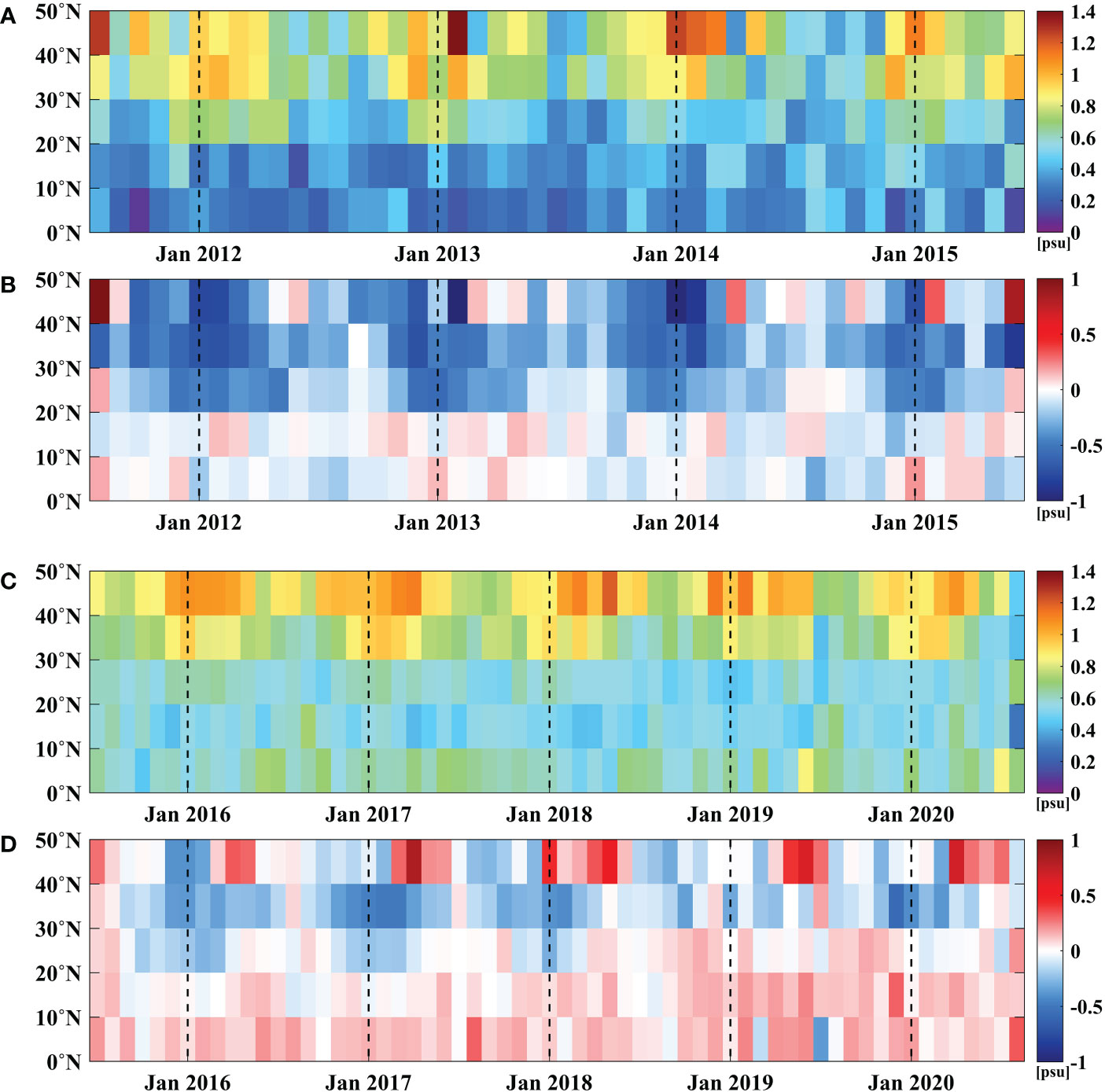
Figure 3 Latitude-time plots of (A) root mean square error (RMSE) and (B) bias of Aquarius sea surface salinity (SSS) (psu) as compared to the in situ salinity measurements in the Northwest Pacific Ocean from August 2011 to June 2015. (C) and (D) are the RMSE and bias of the Soil Moisture Active Passive (SMAP) SSS data from April 2015 to August 2020, respectively.

3.2. Suitability of satellite SSSs for typhoon study

In the previous section, the satellite SSSs in some regions exhibited relatively good RMSE and bias, whereas others revealed poor correlations with the in situ salinity measurements. Therefore, it is important to investigate how the satellite SSSs can be applied to the study of the ocean responses to typhoon forcings. For this purpose, we investigated whether the SSS error over the entire period had a characteristic dependence on the latitude and month.

3.2.1. Limitation on latitude

Figure 4A presents the RMSE-bias plot of the differences between the Aquarius SSS and the Argo salinity with respect to latitude in the Northwest Pacific from 2012 to 2020. Each dotted circle represents a radius (=$\sqrt{RMS{E}^2+bia{s}^2}$) consisting of the RMSE and bias on the x- and y-axis, respectively. The mean error of the Aquarius SSS reached 1.5 psu at high latitudes, particularly in the range of 40–50°N (Figure 4A). Such errors might be attributed to degraded measurement precision and could be improved by averaging with a greater sampling frequency, such as that of a polar orbiting satellite (Vinogradova and Ponte, 2012). However, in tropical and subtropical regions within 20°N from the equator, the errors were greatly reduced and were within a small radius of error (less than 0.5 psu) as illustrated in Figure 4A. In summary, the negative biases were amplified as the RMSE increased (Figure 4A).

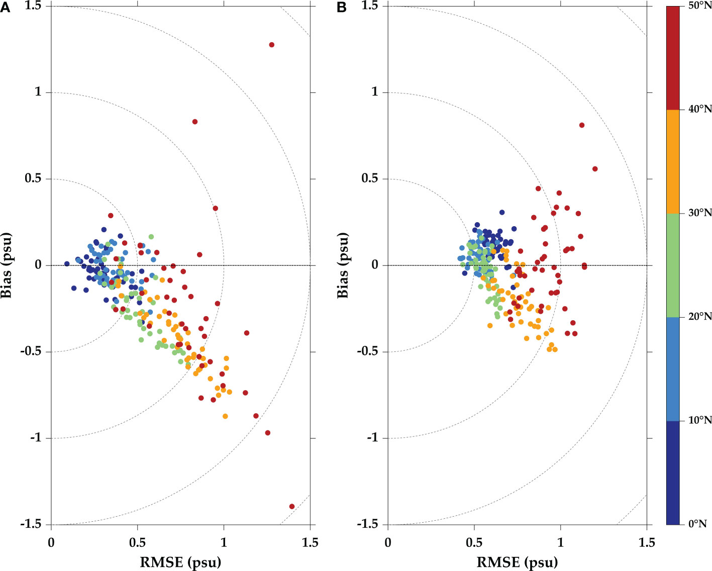
Figure 4 Scatter diagrams of root mean square error (RMSE) and bias between sea surface salinity in (A) Aquarius (August 2011–June 2015), (B) Soil Moisture Active Passive (SMAP) (April 2015–August 2020), and Argo salinity in the Northwest Pacific. Colors represent the latitudes of the matchups from 0°N to 50°N, and the size of each bin is 10 degrees.

Similar to the Aquarius SSS, the SMAP errors in the Northwest Pacific were high with large scattered points within the higher radius of the error circles, and most of the matchups scattered when the radii of the errors were greater than 0.5 psu or more (Figure 4B). Relatively small errors (<0.7 psu) were distributed in the tropical and subtropical regions (<30°N). In contrast, the amplitudes of the errors increased as a function of latitude, amounting to 0.5–0.10 psu at high latitudes (>40°N) (Figure 4B). Thus, we concluded that both the Aquarius and SMAP salinity measurements were relatively accurate in the tropical and subtropical regions within 30°N and inaccurate in boreal regions. This suggests that the responses to typhoons in the subtropical regions can be investigated using the satellite SSS data with a certain uncertainty in their differences.

3.2.2. Limitation on time

The average monthly satellite SSSs were calculated to determine the season with the smallest satellite salinity error. Figures 5A, B show scatter plots of the monthly averaged errors of the Aquarius and SMAP SSSs with error circles in the Northwest Pacific. In both Aquarius and SMAP, the SSS errors indicated a characteristic tendency. Relatively small average errors primarily appeared in the summer, with July having the smallest error, followed by June and August (Figure 5A). Conversely, in winter (January, February, and December), the bias were approximately three times greater than those in the summer as denoted by the three dots on the bottom right.

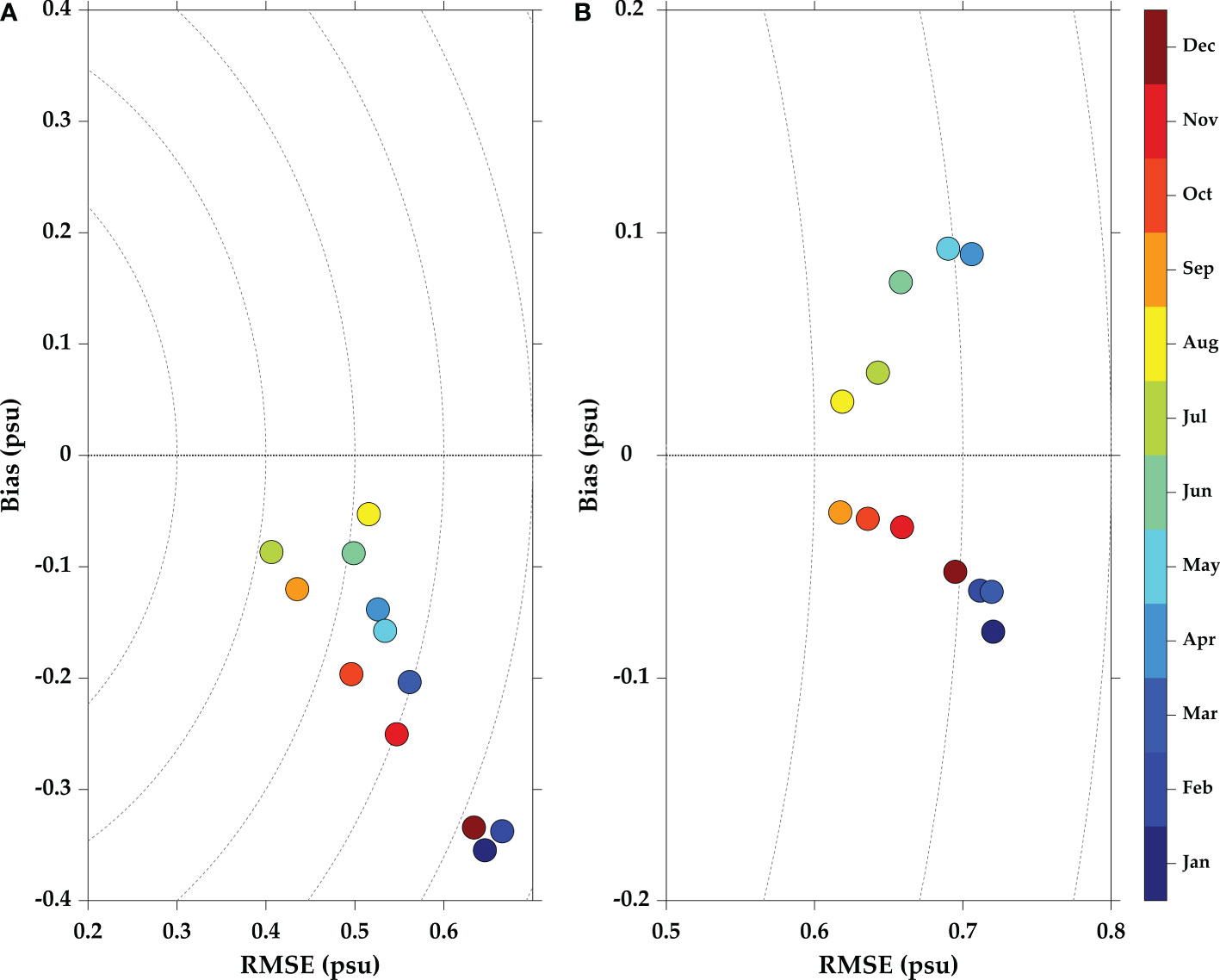
Figure 5 Scatter diagrams of root mean square error (RMSE) and bias between sea surface salinity in (A) Aquarius (August 2011–June 2014), (B) Soil Moisture Active Passive (SMAP) (April 2015–August 2020), and Argo salinity in the Northwest Pacific. Colors represent the months of the matchups from 0°N to 50°N.

In the SMAP satellite, it is likely that there was a slight time delay of a month compared to the results of the Aquarius statellite (Figure 5B). Nevertheless, the SSS errors were still the smallest in the summer season (August and September) and the largest in the winter season (January, February, and March), regardless of the time delay. Therefore, by combining these two results, we concluded that the uncertainty in the satellite SSSs was relatively small in the summer. Our results support the use of the satellite SSS data for the study of typhoons with elevated reliability in the summer as typhoons develop and proceed during that time.

In addition, the satellite salinity data have large errors in cold seawater at high latitudes. The causes of the SSS errors at low SST conditions are associated with the less accurate response of the passive microwave SSS sensors at the L-band frequency, which is in contrast to the high-temperature condition with better measurement precision (Lagerloef and Font, 2010). These satellite salinity error analysis results suggest that the SSS errors are the smallest in summer at low latitudes, where the water temperature is higher compared to that of the high latitudes. Therefore, we applied the satellite SSSs with acceptable accuracy and reliability in our study to investigate the responses to changes in the SSS during the typhoon events.

3.3. Accuracy of satellite salinity and temperature during typhoon events

The results of SSS errors in the previous sections demonstrate that the satellite SSSs produce relatively large errors of approximately 0.2 psu (expected RMSE) or more compared to the in situ salinity measurements. Specifically, these errors are associated with latitude and time. The analysis in the previous section suggested that salinity errors are amplified at high latitudes and therefore are only of use at low latitudes (<30°N) (Figure 4). Furthermore, as shown in Figure 5, the analysis of the temporal variability of the SSS errors suggested that the RMSE was smallest in the summer. One of the oceanographic phenomena that satisfies these conditions may occur during typhoon periods. Therefore, we assessed the accuracy of the SST and SSS during the typhoon periods to demonstrate that the satellite SSS can be of great use in tropical regions during the summer (Figure 6).

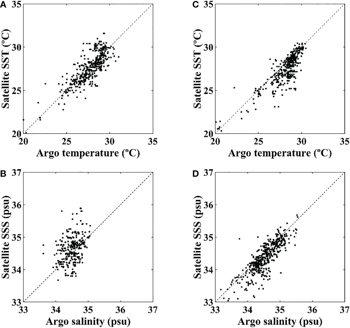
Figure 6 Comparisons of (A) satellite sea surface temperature (SST) (°C), (B) Soil Moisture Active Passive (SMAP) sea surface salinity (SSS) (psu) of the 10 typhoons in the Northwest Pacific from August 2011 to June 2015, (C) satellite SST, and (D) SMAP SSS for the 10 typhoons from April 2015 to August 2020.

The Aquarius satellite-observed SSTs were in agreement with the in situ temperatures observed by the Argo floats with a RMSE and bias of 0.84°C and −0.15°C, respectively (Figure 6A). Similarly, negative bias and RMSE of −0.54°C and 0.82°C, respectively, were yielded from the collocated SMAP SSTs (Figure 6B). The RMSE of the Aquarius SSSs for typhoons was approximately 0.57 psu (Figure 6C), which was a slight improvement compared to the overall RMSE of SSS for all seasons in the Northwest Pacific (Figure 3A). The SMAP SSSs were slightly improved with an RMSE of 0.39 psu and a bias of −0.26 psu from 2015 to 2020 (Figure 3D). The spatial response of the ocean and atmosphere to the typhoons that passed through the Northwest Pacific from 2011 to 2020 will be investigated in the following section with reference to the error characteristics of the satellite data.

3.4. Response of sea water temperature to typhoon

Figure 7A shows the spatial distribution of the minimum SSTs at each spatial grid during Typhoon Wipha from October 10 to 16, 2013. The spatial distribution had a distinct character between the left and right sides from the path of the typhoon center, as indicated by the red line. It curved northwest and moved towards northeast at approximately 25°N. The distance between the adjacent white dots suggests differential movement of the typhoon along the main track every 6 h. The typhoon moved slowly at the beginning, and after passing 25°N, it advanced rapidly to the northwest as it approached the westerly area (Figure 7B). In the region between 15°N and 20°N, the average wind speed to the right of the typhoon was 16 m s^-1.

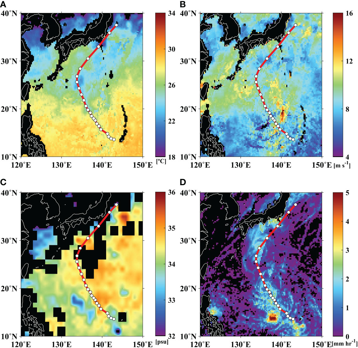
Figure 7 Spatial distributions of (A) minimum of sea surface temperatures (°C), (B) mean of wind speed (m s^-1), (C) minimum Aquarius Sea surface salinity (psu), and (D) mean of precipitation rates (mm h^-1) during Typhoon Wipha passage from 10–16 October, 2013.

Maximum wind speeds above 11 m s^-1 appeared on the right side of the typhoon at relatively low latitudes between 15°N and 25°N. The spatial differences in the wind speed induced differential SST responses at lower temperatures on the right side of the typhoon (Figure 7A). In this region, with high winds, SST cooling of approximately 2°C was observed on the right side of the typhoon, which is consistent with the previous studies (Cornillon et al., 1987; Vincent et al., 2012).

To determine whether this cooling occurred in other typhoons observed by the SMAP satellite, we examined SSTs during Typhoon Champi passage from 13–25 October, 2015. Figure 8A shows the spatial distribution of minimum SSTs calculated at a given point in the Northwest Pacific during the typhoon passage. In the vicinity of 20°N, substantial SST cooling occurred on the right side close to the typhoon path with enhanced asymmetry. Around 25°N or higher, relatively low SSTs appeared further away to the right side of the typhoon center. Figure 8B exhibits the distribution of the mean temporal wind speed during the typhoon period. Relatively strong wind speeds were distributed to the right of Typhoon Champi. Such dominant sea surface cooling responses were due to the strong vertical mixing of typhoons.

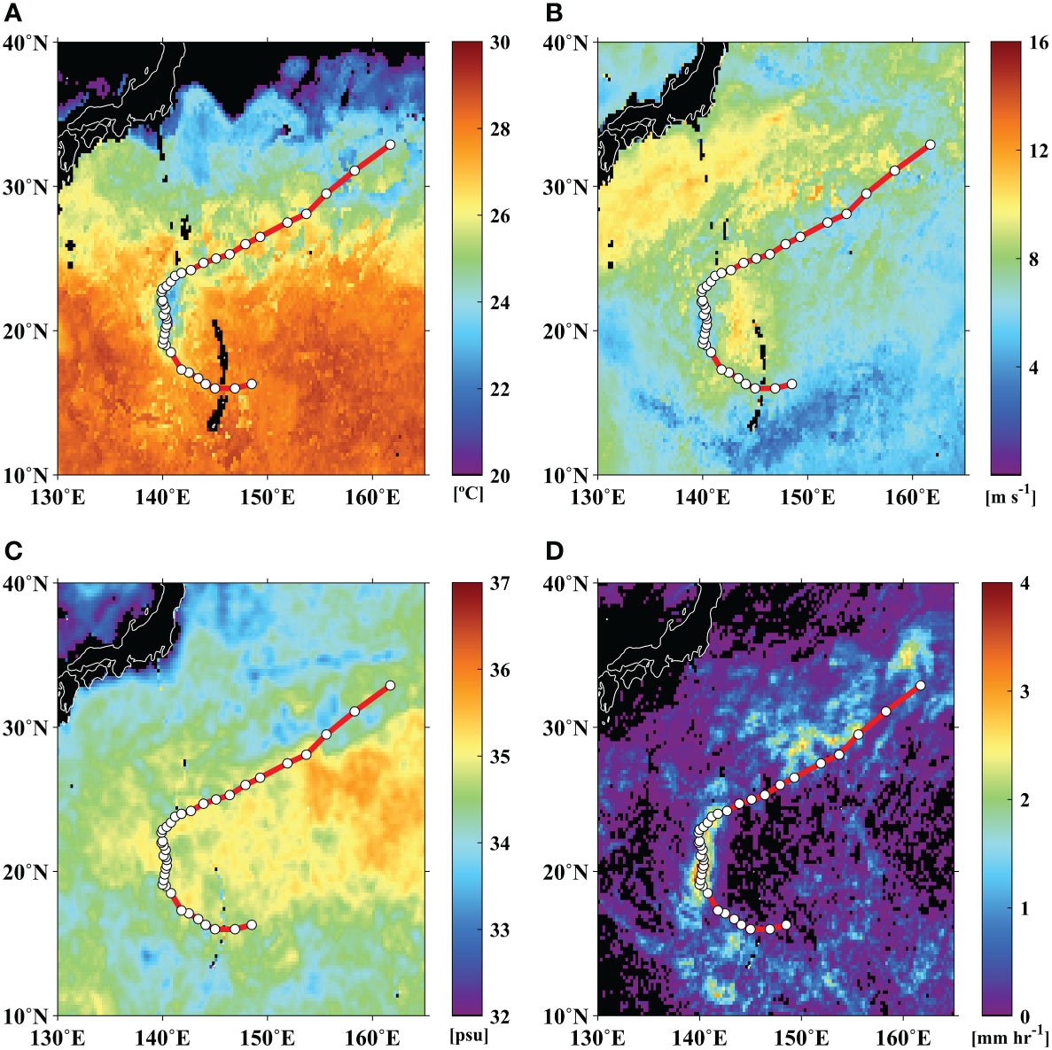
Figure 8 Spatial distributions of (A) minimum sea surface temperatures (°C), (B) mean of wind speed (m s^-1), (C) minimum SMAP sea surface salinity (psu), and (D) mean of precipitation rates (mm h^-1) during Typhoon Champi passage from 13–25 October, 2015.

3.5. Response of sea surface salinity

To investigate the effect of typhoons on salinity distribution, we analyzed the Aquarius SSS by calculating the minimum SSS during Typhoon Wipha passage (Figure 7C). A low salinity of approximately 33.5 psu appeared west to the central track of the typhoon at 13–19°N latitudes. This pattern was clearly in contrast to that of 34.5 psu on the eastern side. The zonal difference in salinity across the typhoon center amounted to 1.0 psu. A similar tendency was detected during the initial stage of the typhoon at ~11°N latitudes (Figure 7C). However, as the typhoon moved closer to land, salinity data could not be obtained due to thick clouds and extremely strong precipitation in the westerly wind region. This resulted in many missing pixels of the Aquarius SSS, as denoted in black near the typhoon passage. During Typhoon Champi, the SMAP SSS revealed weak freshening on the left side and saline responses on the right side (Figure 8C).

The upper ocean response observed by satellite data can be observed from the in situ salinity measurements near the sea surface by Argo floats (Park et al., 2005). Figures 9A, C shows a scatter plots of the Argo temperatures at depths (approximately 3–5 m) nearest to the surface, which were obtained near the typhoon tracks of Wipha and Champi within 24 h. The Argo SST indicated weak surface cooling on the right side at latitudes >30°N compared to that on the left side. Notable freshening (34.2 psu) on the left side of Typhoon Wipha was observed at latitudes <20°N, particularly during the initial stage from October 10 to 13, 2013, in the Argo salinity (Figure 9B). The high salinity points above 34.8 psu on the right side of the typhoon are in contrast with the dominant freshening with a low salinity of approximately 34.2–34.4 psu on the left side.

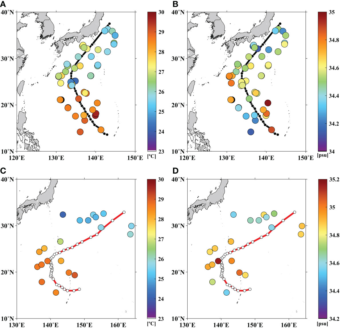
Figure 9 Scatter plots of (A) surface temperature (°C) and (B) surface salinity (psu) observed by Argo float during Typhoon Wipha from 10–16 October, 2013. (C) and (D) are the same as (A) and (B) for Typhoon Champi from 13–25 October, 2015. The black and red lines represent the typhoon tracks.

During Typhoon Champi, the Argo data exhibited that the SMAP SSS freshening occurred on the left of the typhoon. In the early stage of the typhoon, the salinity (34.6 psu) near 16°N was at least 0.2 psu lower than that of the surrounding area (Figure 9D). The trend of spatial differences in typhoon-driven salinity changes is consistent with the satellite salinity observations, as noted above. This emphasizes that the salinity measurements by satellites can be of great use in studying the oceanic responses to typhoons.

3.6. Changes in vertical structure

The changes in vertical structure of temperature and salinity from Argo floats after the typhoon events are shown in Figure 10. The temperature profile at a specific location (24.86°N, 134.44°E) before the landing of the typhoon Wipha on 6 October 2013 showed an almost constant temperature of about 28.3°C in the mixed layer to 40 m as indicated by the red line in Figure 10A. After the typhoon passed, the vertical profile at a distance of about 57.7 km from the previous location (25.15°N, 134.85°E) shifted a temperature of about 24.1°C, more than 4°C lower than the previous profile, as indicated by the blue line in Figure 10A. An obvious deepening of the mixed layer depth from 40 m to 70 m was indicated after the typhoon Wipha passed. The temperature difference (post minus previous) varied by −4.2°C at the upper layer at (<50 m) (Figure 10B).

Figure 10 Vertical profiles of (A) Argo temperature (°C), (B) temperature difference (°C), (C) Argo salinity (psu), and (D) salinity difference from Argo measurements before and after Typhoon Wipha passage. (E–H) are the vertical profiles of Typhoon Champi in the Northwest Pacific.

The vertical Argo profile of salinity demonstrated an obvious oceanic response of freshening, as shown by the shift of the red line at a location (14.43°N, 135.61°E) on 7 October 2013 to the blue line at (14.18°N, 136.07°E) on October 16 before and after the typhoon Wipha, respectively (Figure 10C). The surface salinity changed by 0.3 psu, from 34.43 psu to 34.13 psu, as a result of the typhoon activity. The freshening amounted to 0.29 psu at the upper layer of the sea surface to 40 m (Figure 10D). These changes in Argo temperature and salinity profiles of the surface layer show good agreement with the satellite measurements, as shown earlier in Figures 7 and 8. In situ glider observation in previous studies showed deepening of the mixed layer and salinity reduction of 0.15 psu at depths of up to 80 m (Hsu and Ho, 2019), as well as a salinity decrease of approximately 0.074–0.152 psu (Liu et al., 2020). Yue et al. (2018) also pointed out a salinity decrease of 0.02–0.41 psu above 70 m on the left side of typhoons.

For the typhoon Champi, the Argo temperature and salinity data prior to and post the typhoon passage were compared by using the two profiles at 20.36°N, 135.86°E on 9 October 2019 and 17.87°N, 137.40°E on 21 October. Argo temperatures of the mixed layer were slightly decreased by about –0.3 psu within upper 60 m layer (Figures 10E, F). Salinity freshening was also detected by –0.2 psu from 34.9 psu to 34.7 psu within a mixed layer of about 60 m thickness (Figures 10G, H).

3.7. Relation of SSS and precipitation

The mechanism of spatial differential freshening on the left side of the typhoon center might have been caused by the precipitation around the typhoon (Yue et al., 2018; Hsu and Ho, 2019; Liu et al., 2020). Figure 7D shows the spatial distribution of the mean precipitation rate at each location, averaged over the typhoon period. It revealed overall rainfall rates over 2.5 mm h^-1 in the left side, with high precipitation mean amounting to 5 mm h^-1 during the early passage of the typhoon on October 11, 2013. The location of the strongest rainfall rate was not coincident with the lowest SSS, however, it was located near the highest response of salinity, as shown in Figures 7C, D. Figure 8D demonstrates that the precipitation was much higher in the left side throughout the entire period of Typhoon Wipha. The overall precipitation rate on the left side was approximately thrice of that on the right side. According to the theoretical model of atmospheric conditions, the core of the intensive rainfall was apparent on the forward left side of the typhoon (Lonfat et al., 2004). Thus, the rainfall pattern manifested in the spatial distinction between the left and right sides reflects the actual atmospheric conditions during the typhoon passage. This tendency was also observed in Typhoon Champi (Figures 8C, D). Along the entire path of the typhoon, the salinity on the left side was much lower than that on the right side, whereas the precipitation was higher than that on the right side. Thus, this asymmetry of precipitation between the left and right sides may be the source of the differential SSS distribution across the typhoon center.

To examine the relationship between the salinity difference and the precipitation, we analyzed a composite of zonal profiles of the salinity values from 135°E to 145°E and the precipitation during Typhoon Wipha by investigating the averages along latitudes between 10°N and 20°N (Figure 11A). A high peak of precipitation, denoted by the red line in Figure 11A, was detected on the left side of the typhoon, approximately 180 km from the typhoon center. In summary, the left side had a mean precipitation rate of 7.66 mm h^-1 within 400 km distance from the typhoon center, which was considerably higher (61.57%) than that on the right side (4.74 mm h^-1). The mean value of the satellite SSS on the left side was 33.59 psu, which was remarkably lower than that on the right side (1.35 psu). A cross-section of the satellite SSS along the same zonal lines showed it was considerably lower, with a peak value of approximately 33.2 psu on the left side. The relationship between the SSSs and the precipitation rates exhibited a slope of −0.0261 psu mm^-1 h^-1 (Figure 11B), which was lower than the freshening bias of −0.05 psu mm^-1 h^-1 described by Meissner et al. (2014). As the precipitation increased, the satellite-observed SSS decreased, leading to surface freshening as the typhoon passed.

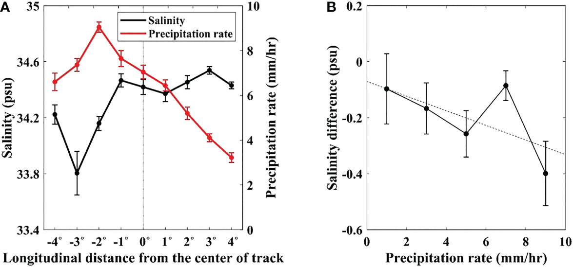
Figure 11 (A) Zonal distribution of sea surface salinity (a black line) (°C) and precipitation rate (a gray line) (mm h^-1) across Typhoon Wipha track at a cross section within a range of 10–20 °N, 130–150 °E, and (B) relationship between satellite salinity difference (after minus before the arrival of Typhoon Wipha) and precipitation rate.

3.8. Response across typhoon center

In the previous sections, examples of the oceanic responses to Typhoon Wipha were presented. To confirm and generalize the results, we investigated the statistical results of other typhoons using the Aquarius and SMAP data. A total of 20 typhoons were included to meet the criteria for the analysis of the response statistics, as illustrated in Figure 12.

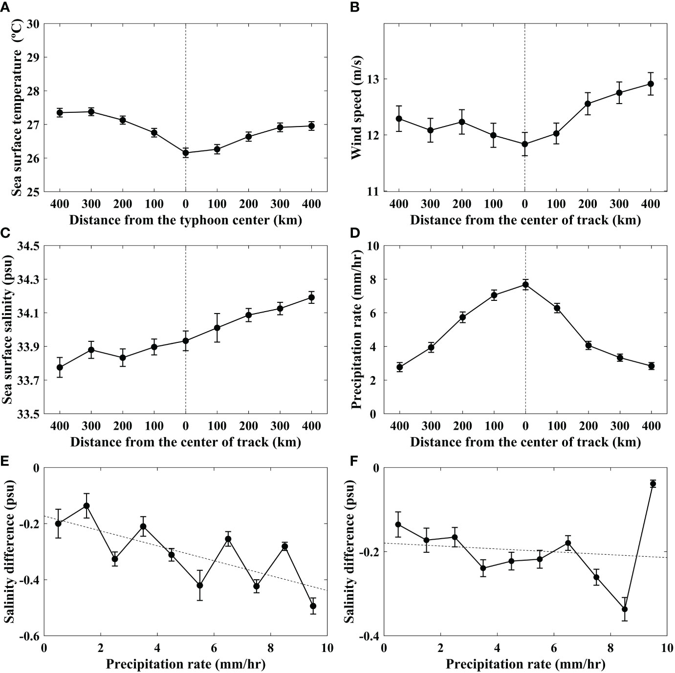
Figure 12 Distributions of (A) SST (°C), (B) wind speed (m s^-1), (C) salinity (psu), and (D) precipitation rate (mm h^-1) as a function of distance from a typhoon center in the Northwest Pacific. SSS difference (Aquarius – Argo) as a function of the maximum precipitation rate over time in (E) the left and (F) right side of each typhoon, where the error bar represents a mean error ($\sigma /\sqrt{N-1}$)), N is the number of the matchup data points in each interval, and the dashed line represents a least-squared linear fit.

Typhoons are accompanied by extreme atmospheric and oceanic conditions. Thus, many satellite observations become heavily contaminated due to backscattering or absorption attributed to heavy rainfall or unknown causes (Kaufman et al., 2005). Such severe conditions result in insufficient satellite measurements for examining the upper ocean responses to typhoons. Therefore, we took the averages of satellite-observed oceanic and atmospheric variables, such as the SSTs, wind speeds, SSSs, and precipitation rates, for the regions near the typhoon during its entire lifetime, as illustrated in Figure 12. The SST distribution indicated spatially differential cooling on the right sides of 10 typhoons compared to the left sides (Figure 12A), which is consistent with previous studies (Cornillon et al., 1987; Sakaida et al., 1988; Wada, 2005; Jiang et al., 2006), The mean Aquarius SST of 10 typhoons on the right side was approximately 26.8°C at distances of 0–300 km from the typhoon center, which was in contrast to the high SST of approximately 28°C far from the typhoon center. This might be attributed to the higher mean wind speeds (>12 m s^-1) on the right side than on the left side, as addressed in previous studies (Price, 1981; Shay et al., 1992; Monaldo et al., 1997; Lin et al., 2003; D'Asaro et al., 2011) (Figure 12B).

Figure 12C shows the Aquarius SSS distributions averaged over 10 typhoons as a function of the distance from the center of each typhoon. The mean SSS value on the left side was approximately 33.38 psu, which was 0.62 psu lower than that on the right side (34.0 psu) (Figure 12C). The lowest peak of salinity coincided with the highest peak of precipitation rate (approximately 4.66 mm h^-1) at a distance of 0–100 km on the left side of the typhoon (Figure 12D). As the precipitation rate increased, the satellite SSSs decreased as hypothesized. To examine the role of precipitation in SSS changes, the maximum precipitation rates for a 3-day period were compared with the satellite SSS differences before and after the passage of each typhoon. The satellite SSS differences (values before the typhoon minus those after its passage) in 10 typhoons decreased at a rate of −0.1610 psu mm^-1 h^-1 (p = 1.0×10⁻³) on the left side of typhoons (Figure 12E), indicating that freshening of the SSS strengthened as rainfall increased. Similar freshening was detected on the right side at a lower rate of −0.0904 psu mm^-1 h^-1 (p = 8.3×10⁻³). These decreasing trends are in reasonable agreement with the freshening bias of −0.05 psu mm^-1 h^-1 reported previously (Meissner et al., 2014). As precipitation increased, the Aquarius-observed SSS decreased, leading to freshening near the typhoon. The oceanic responses of this type exhibited good agreement with the analyses of the Argo data and the results of model simulations reported in previous studies (Sun et al., 2012; Liu et al., 2014; Sun et al., 2015).

To confirm whether this trend was consistent in the SMAP data, 10 typhoons were selected and analyzed. Results confirmed that the SMAP SSSs responded to the typhoons similarly as the Aquarius SSSs (Figure 13). Averaging the variables of 10 typhoons showed that the SST was 27.08°C and approximately 26.46°C on the left and right (within 500 km from the center of the typhoon) side, respectively (Figure 13A). This trend coincided with the distribution of winds on the right side, with an average wind speed of 11.86 m s^-1, which was higher than that on the left (11.05 m s^-1) (Figure 13B). The average SSS on the left side was 34.27 psu, which was considerably lower than that on the right side (34.55 psu) (Figure 13C). This was consistent with the asymmetric distribution of precipitation at 4.6 mm h^-1 and 3.52 mm h^-1 on the left and right side, respectively (Figure 13D). The rate of change of salinity with respect to precipitation decreased to −0.0141 psu mm-1 hr^-1 as the precipitation rate increased on the left side of the typhoon (Figure 13E). This rate was similar to the result of Yue et al. (2018), who reported that a rain rate of 6.8 mm h^-1 led to a salinity decrease of 0.02–0.41 psu above 70 m on the left side of typhoons. In contrast, there was a slight increase on the right side, however, it was much lower than that on the left side by O(1) and did not have any statistical significance (Figure 13F).

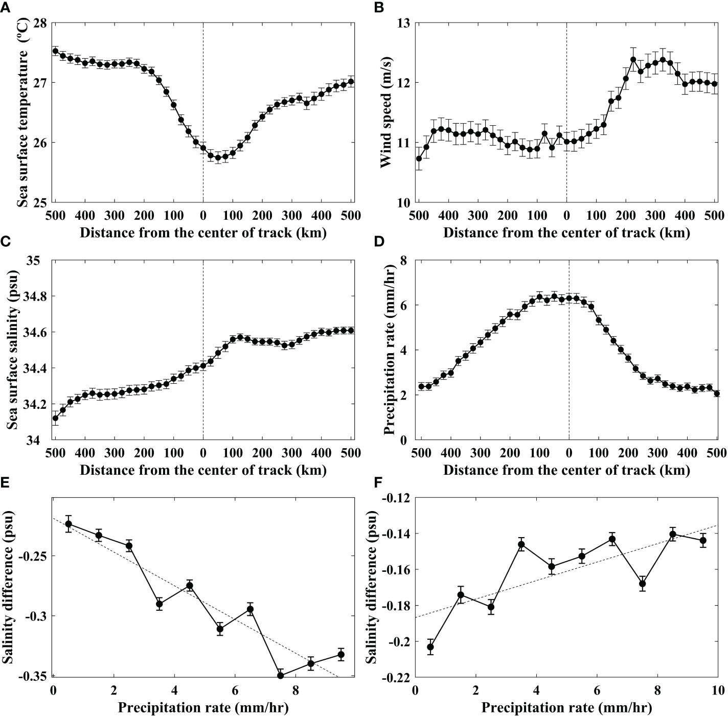
Figure 13 Distributions of (A) SST (°C), (B) wind speed (m s^-1), (C) salinity (psu), and (D) precipitation rate (mm h^-1) as a function of distance from a typhoon center in the Northwest Pacific. SSS difference (SMAP – Argo) as a function of the maximum precipitation rate over time in (E) the left and (F) right side of each typhoon, where the error bar represents a mean error ($\sigma /\sqrt{N-1}$), N is the number of the matchup data points in each interval, and the dashed line represents a least-squared linear fit.

4. Discussion

4.1. Spatial structure of environment near the typhoon center

Although it is known that typhoons decrease the SST due to strong winds on the right side of their center, the extent to which the typhoons influence the changes in salinity, rain rate, wind, and water moisture around their center remains unclear. Therefore, for understanding the typhoon-related phenomena comprehensively, it is necessary to analyze the oceanic responses around the center of the typhoon in a 2-D synoptic view as typhoons are spatially distributed over a wide area. As seen previously, salinity freshening was detected on the left side of the typhoon center. However, each tropical storm has a characteristic path with extensive spatial and temporal variability. Our findings raise questions about the credibility of severe freshening sites related to prominent rainfall sites. Therefore, the environmental changes around the typhoons were investigated by transforming the coordinates such that the path of typhoon direction was upward (90°), and the differences in response after the typhoon passed were examined and discussed.

Figure 14 shows the spatial distribution of the oceanic and atmospheric variables in the rotated coordinate system with a particular focus, where the upward direction coincided with the moving direction of the typhoon. The coordinate transformation provided additional insights for a fundamental understanding of the oceanic responses around the typhoon center and its passage. The x-axis and y-axis of each plot in Figure 14 represent the distance ratio of the left/right side and front/behind distances from the center of the typhoon, respectively, divided by the radius of the typhoon’s maximum wind gust. For the typhoons observed by the Aquarius satellite (Table 1), the average SST was in the range of 25.0–26.0°C at a distance of approximately 1.0 r/R_max (r: distance from the center, R_max: radius with maximum wind speed) from the center of the typhoon, which was in contrast to the surrounding SSTs (27.0–28.0°C) (Figure 14A). The SSTs near the center were relatively low, with more enhanced cooling on the right side of the typhoon, as noted in numerous studies (e.g., Cornillon et al., 1987).

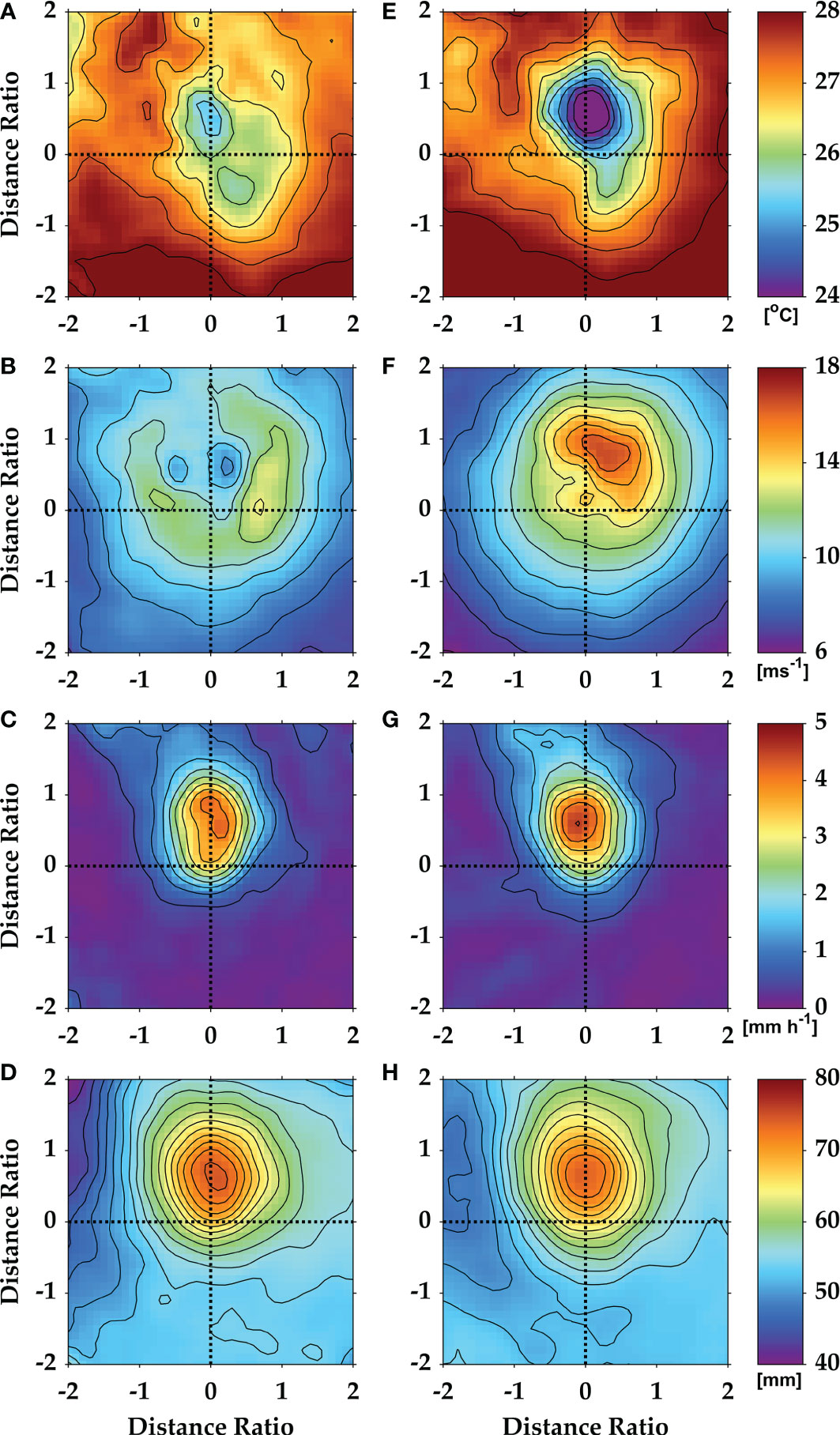
Figure 14 Spatial distributions along-typhoon components of (A) SST (°C), (B) wind speed (m s^-1), (C) precipitation rate (mm h^-1), and (D) total column water vapor (or total precipitable water vapor) (mm) in the rotational coordinate system as a function of distance ratio from a typhoon center in the Northwest Pacific using Aquarius data. (E–H) are the cases using SMAP data.

In general, the wind speed on the right side of the typhoon center is stronger than that on the left side. The average pattern of typhoons observed by the Aquarius satellite showed higher wind speed of 12.0–14.0 m s^-1 on the right side near r_x/R_max of 1 (r_x: a zonal distance from the center) than near the typhoon center (low wind speed of ~8.0 m s^-1) (Figure 14B). However, the maximum value of precipitation existed in the vicinity of 0.8–0.9 r_y/R_max (r_y: a meridional distance from the center) in the forward moving direction of the typhoon (Figure 14C). The water vapor distribution was circular, with the largest peak in the forward direction of the typhoon, a sharp decrease on the left side, and a smooth decreasing extension on the right side of the typhoon center (Figure 14D). When the water vapor rises upward toward the typhoon center due to strong winds, a phase change that generates latent heat occurs, which plays an important role in the development and evolution of typhoons. Since water vapor is used as an energy source south of the typhoon center, it is assumed that there is a relatively low water vapor content behind the typhoon. Precipitation is extensive in areas with a large amount of water vapor in front of the typhoon.

Results of the SMAP data analysis exhibited similar results as Aquarius to the environmental and oceanic responses around the typhoon. In the typhoons observed by SMAP, a much larger SST cooling occurred than that of Aquarius on the forward and right sides of the typhoons at overall approximately 24–25 °C (Figure 14E). The maximum wind gust appeared at r_y/R_max (0.8–1.0) in the forward direction and right side of the typhoons, with an overall stronger pattern (r_x/R_max ~ 0.5) than on the left side (Figure 14F). Similarly, the spatial pattern of rainfall revealed that there was an intensive rainfall area on the weakly left (r_x/R_max = –0.1) and forward region (r_y/R_max = 0.8–0.9) from the typhoon center (Figure 14G). In the spatial distribution of water vapor, there was a peak at similar forward locations (0.5< r_y/R_max <1) from the center of the typhoon, similar to the results of Aquarius (Figure 14D).

Our results are consistent with the results of observations and simulations of the spatial structure of tropical cyclones. The rain shield is reported to be well-developed in the northern half of the typhoon system (Fogarty, 2002). Water vapor condenses to generate latent heat and is used as an energy source for the development of a tropical cyclone and its movement. Therefore, changes in the atmospheric environment around the typhoon center based on the satellite data are consistent with the results of the model simulations and observations, implying that satellite data can be used to reveal some degree of ocean response even in extreme conditions, such as typhoons.

4.2. Spatial structure of salinity response around the typhoon center

As illustrated earlier, the environment along the direction of the typhoon passage exhibited that the maximum precipitation core was located slightly to the forward left part. This spatial distribution of precipitation produced a differential distribution of salinity around the typhoon center. Therefore, by analyzing the spatial structure of the salinity response, we investigated the relationship between the precipitation and satellite SSS distribution using swath data from satellite salinity observations at each pixel, instead of temporally averaged gridded salinity data. In the Aquarius SSS, the amount of swath data was not sufficient. Therefore, only SMAP data with high spatial sampling frequency were used to investigate the salinity response in the along-track coordinates that slowed the typhoon movement.

Figure 15A shows the average SSS field around the typhoon centers in the non-rotated system without coordinate transformation. Satellite SSS was distributed in the overall range of 33.5–36.0 psu, and relatively large salinity of 35.0–36.0 psu was distributed in most areas northeast of the typhoon center. Salinity was relatively low at approximately 34.0 psu southwest of the typhoon center, and the minimum value (< 34.0 psu) was shown at 150 km west of the typhoon. As this average field contained different responses depending on the direction of each typhoon, the responses surrounding the typhoon were investigated by tracking the directions of the typhoons (Figure 15B). The mean distribution of rotated salinity was much higher (1–1.5 psu) in the east of the moving directions due to the salinity enhancement by vigorous evaporation because of the strong wind speed on the right side of the typhoons. The evaporation process also magnified the changes in the salinity. Relatively low salinity values appeared in the forward (R_y/R_max= 0.3–0.8) and weakly to the left side (R_x/R_max= 0.1) of the typhoon center. This was consistent with the location of the salinity minimum core shown in Figure 14G. The difference between the minimum and maximum salinity values around the typhoon was approximately 2.5 psu. These findings are in good agreement with those of previous studies, such as the schematic diagram of hurricanes (Fogarty, 2002). As the typhoon progressed, dry air existed on the left side of the typhoon, and large amounts of water vapor were present on the foreside of the typhoon, forming an intensive precipitation band. The core of the precipitation zone was distributed on the left side of the typhoon, as shown in Figure 14G. The higher salinity values on the right side demonstrate that strong winds have a much greater effect on the salinity changes in the eastern region than precipitation. Therefore, we estimated that the spatial distribution patterns of wind speed and precipitation bands were combined to show a spatially specific response pattern of the SSS around the center of the typhoon (Figure 15B). All of these results provide insight into understanding the two-dimensional and synoptic feature of oceanic and atmospheric environments around the tropical strom center.

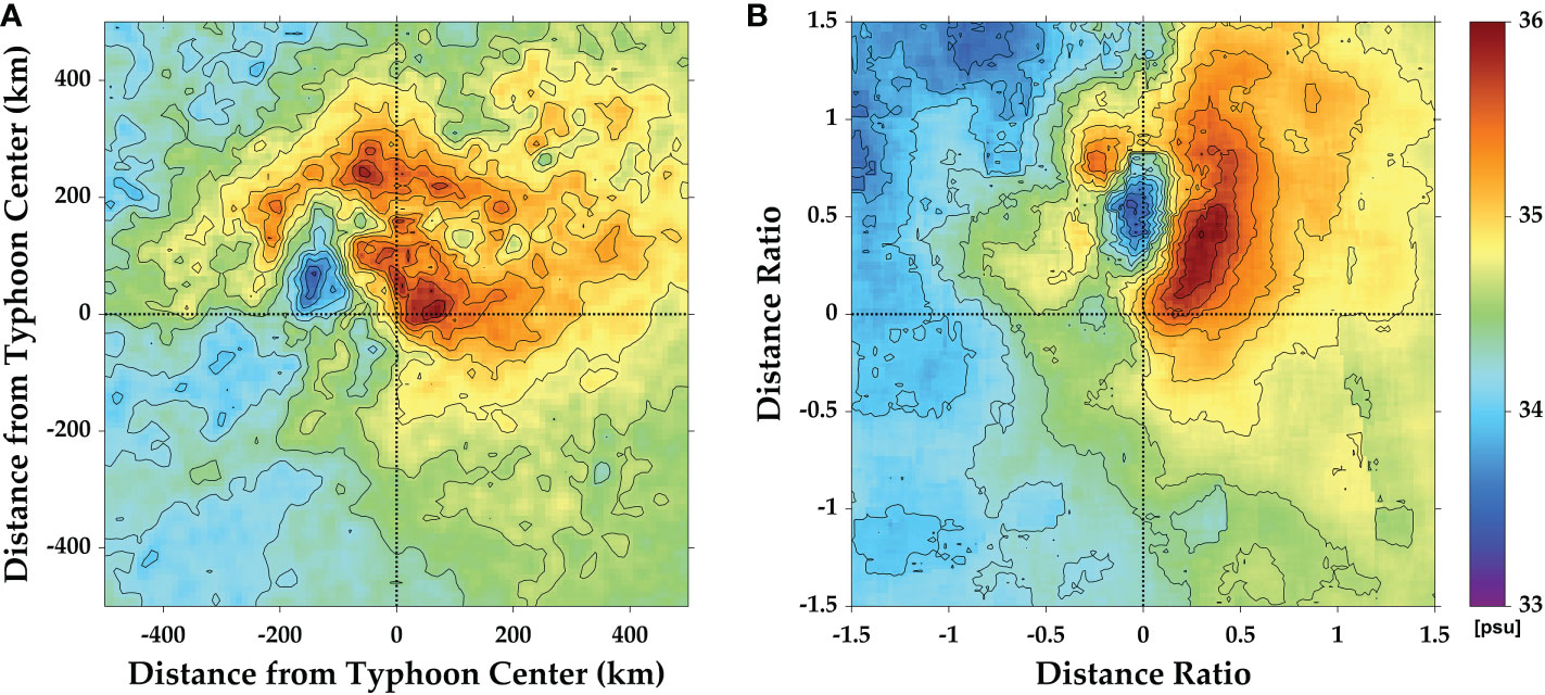
Figure 15 Spatial distributions of sea surface salinity (psu) responses in (A) non-rotated and (B) rotated coordinates in the direction of typhoons as a function of distance ratio from the typhoon center in the Northwest Pacific using SMAP data.

5. Conclusion

Changes in the SSS have major effects on the flow of oceanic currents through changes in seawater density and control of heat and circulation movement. Typhoon-driven freshening of the SSS can lead to changes in the vertical stratification of seawater, thereby affecting the local marine ecosystem. To further understand the mechanisms of typhoon-caused forcings and oceanic responses, we investigated the accuracy of the satellite SSS in the Northwest Pacific over the past decade (2011–2020) by comparing it with the in situ salinity measurements from the Argo float measurements. The satellite SSS errors of the Northwest Pacific Ocean presented a characteristic dependence on the latitude. The errors tended were reduced in the low-latitude tropical regions, where typhoons developed. In addition, the SSS errors were relatively small in the summer.

Despite such uncertainties in the SSS values, satellite-observed SSSs in the subtropical regions exhibited more surface freshening on the left side of the typhoon compared to the center of the typhoon. The spatial distinction of surface freshening on the left side of the typhoon coincided with that of the higher precipitation rates on the same side. The differential spatial distribution of the SSS was considerably related to that of the precipitation rates. The SSSs were affected by a precipitation rate of approximately −0.04 psu mm^-1 h^-1. The freshening did not always appear during the entire period of the typhoon, however, it was clearly indicated during its initial stage with the slow movement of typhoons at 10–20°N in the Northwest Pacific. The Argo profile data explained the vertical changes in temperature and salinity, such as the processes of deepening, cooling, and freshening mechanisms of the mixed layer after the typhoon passage, which was consistent with the analysis results of the satellite SSS observations.

However, a partial correlation between the satellite and Argo SSS does not signify that satellite salinity can be directly applied over the entire ocean region. The method still has many limitations in latitudinal regions (>40°N), with very low water temperatures. Therefore, satellite SSS should be used with caution in other applications. One of the objectives of our study was to determine the possibility of using the satellite SSS data in typhoon research. Despite the freshening of surface water during the typhoon periods presented in our study, the limitations in satellite salinity data can prevent universal usage. Nevertheless, the accuracy and error characteristics of the SSS disclosed herein are expected to enhance our understanding of the potential sources of SSS variations and freshening in the Northwest Pacific during typhoon passages. We found that a circular core with a high water vapor content existed in the front part of the typhoon direction in the along-typhoon coordinate system. In the SMAP observations, the positions of the two cores with high precipitation rates and low salinity appeared in the front and slightly to the left of the typhoon paths, showing a significant correlation. In addition, relatively high salinity was observed on the right side of the typhoons, where the wind speeds increased considerably. This was caused by a vigorous evaporation process due to prominent winds on the right side of the typhoons. The correlation between the environmental variables surrounding the typhoons demonstrated the dynamic ocean-atmosphere interactions and salinity responses of the seawater along the path of each typhoon during the past two decades. These findings coincide with previous results that rainfall is concentrated ahead of and to the left of the storm and much less to the right of the track because of the intrusion of dry air from the southern part (Klein et al., 2000; Fogarty, 2002; Fogarty and Region, 2002)

Better SSS estimates under high SSTs and low-latitude regions will provide preferable conditions for typhoon research. Continued validation of satellite SSS has the potential to further enhance the investigation of the oceanic responses to typhoons. The usefulness of satellite salinity measurements for studying oceanic phenomena has been partly limited by uncertainties and errors. Nevertheless, our study provided reasonable observational evidence of oceanic responses to typhoons in the Northwest Pacific. It will further contribute to the understanding of atmospheric and oceanic processes related to tropical storms or hurricanes in any region for future in-depth and diverse studies.

Data availability statement

Publicly available datasets were analyzed in this study. This data can be found here: https://podaac.jpl.nasa.gov, www.remss.com, ftp://ftp.ifremer.fr/ifremer/argo, https://www.nodc.noaa.gov.

Author contributions

K-AP conceptualized, organized, analyzed the datasets, prepared figures, and wrote the manuscript. J-JP analyzed the salinity datasets and prepared the figures, and WT revised the manuscript. All authors contributed to the article and approved the submitted version.

Funding

This study was supported by the National Research Foundation of Korea (NRF), grant funded by the Korean government (MSIT) (No. 2020R1A2C2009464).

Acknowledgments

Argo data were provided by NOAA NODC from https://www.nodc.noaa.gov. AMSR-2 data were obtained from the web site of Remote Sensing Systems (https://www.remss.com) and were sponsored by the NASA AMSR-E Science Team and the NASA Earth Science MEaSUREs Program. The authors thank NASA JPL (https://podaac.jpl.nasa.gov) for providing satellite salinity data. Salinity validation work was partly supported by the IORS project of the Korea Hydrographic and Oceanographic Agency and ‘Korea Institute of Marine Science & Technology Promotion (KIMST) (20220541)’ project by the Ministry of Oceans and Fisheries, Korea.

Conflict of interest

The authors declare that the research was conducted in the absence of any commercial or financial relationships that could be construed as a potential conflict of interest.

Publisher’s note

All claims expressed in this article are solely those of the authors and do not necessarily represent those of their affiliated organizations, or those of the publisher, the editors and the reviewers. Any product that may be evaluated in this article, or claim that may be made by its manufacturer, is not guaranteed or endorsed by the publisher.

References

Abe H., Ebuchi H. (2014). Evaluation of sea surface salinity observed by aquarius. J. Geophys. Res. 119, 8109–8121. doi: 10.1002/2014JC010094
Bao S., Wang H., Zhang R., Yan H., Chen J. (2019). Comparison of satellite-derived sea surface salinity products from SMOS, aquarius, and SMAP. J. Geophys. Res. Oceans 124, 1932–1944. doi: 10.1029/2019JC014937
Bhaskar T. V., Jayaram C. (2015). Evaluation of aquarius sea surface salinity with argo sea surface salinity in the tropical Indian ocean. IEEE Geosci. Remote Sens. Lett. 12, 1292–1296. doi: 10.1109/LGRS.2015.2393894
Bingham F. M., Howden S. D., koblinsky C. J. (2002). Sea Surface salinity measurements in the historical database. J. Geophys. Res. 107 8019. doi: 10.1029/2000JC000767
Bond N. A., Cronin M. F., Sabine C., Kawai Y., Ichikawa H., Freitag P., et al. (2011). Upper ocean response to typhoon choi-wan as measured by the kuroshio extension observatory mooring. J. Geophys. Res. Oceans 116, C2. doi: 10.1029/2010JC006548
Boutin J., Martin N., Reverdin G., Yin X., Gaillard F. (2013). Sea Surface freshening inferred from SMOS and ARGO salinity: Impact of rain. Ocean Sci. 9, 183–192. doi: 10.5194/os-9-183-2013
Chen L., Li J., Tang Y., Wang S., Lu X., Cheng Z., et al. (2021). Typhoon-induced turbulence redistributed microplastics in coastal areas and reformed plastisphere community. Water Res. 204, 117580. doi: 10.1016/j.watres.2021.117580
Conkright M. E., Locarnini R. A., Garcia H. E., O'Brien T. D., Boyer T. P., Stephens C., et al. (2002). World ocean atlas 2001: Objective analyses, data statistics, and figures: CD-ROM documentation. (Silver Spring, MD: National Oceanographic Data Center).
Cooper S. N. (1988). The effect of salinity on tropical ocean model. J. Phys. Oceanogr. 18, 697–707. doi: 10.1175/1520-0485(1988)018<0697:TEOSOT>2.0.CO;2
Cornillon P., Stramma L., Price J. F. (1987). Satellite measurements of sea surface cooling during hurricane Gloria. Nature 326, 373–375. doi: 10.1038/326373a0
Curry R., Dickson B., Yashayaev I. (2003). A change in the freshwater balance of the Atlantic ocean over the past four decades. Nature 426, 826–829. doi: 10.1038/nature02206
D'Addezio J. M., Subrahmanyam B. (2016a). Sea Surface salinity variability in the agulhas current region inferred from SMOS and aquarius. Remote Sens. Environ. 180, 440–452. doi: 10.1016/j.rse.2016.02.006
D'Addezio J. M., Subrahmanyam B. (2016b). The role of salinity on the interannual variability of the Seychelles-chagos thermocline ridge. Remote Sens. Environ. 180, 178–192. doi: 10.1016/j.rse.2016.02.051
D'Asaro E. A., Black P., Centurioni L., Harr P., Jayne S., Lin I. I., et al. (2011). Typhoon-ocean interaction in the western north pacific: Par 1. Oceanography 24, 24–31. Available at: http://www.jstor.org/stable/24861117.
D'Asaro E. A., Sanford T. B., Niiler P. P., Terrill E. J. (2007). Cold wake of hurricane frances. Geophys. Res. Lett. 34, 15. doi: 10.1029/2007GL030160
Drucker R., Riser S. C. (2014). Validation of aquarius sea surface salinity with argo: Analysis of error due to depth of measurement and vertical salinity stratification. J. Geophys. Res. 119, 4626–4637. doi: 10.1002/2014JC010045
Durack P. J., Wijffels S. E., Matear R. J. (2012). Ocean salinities reveal strong global water cycle intensification during 1950 to 2000. Science 336, 455–458. doi: 10.1126/science.1212222
Emanuel K. A. (1991). The theory of hurricanes. Annu. Rev. Fluid Mech. 23179–196, 1991. doi: 10.1146/annurev.fl.23.010191.001143
Emanuel K. (2001). Contribution of tropical cyclones to meridional heat transport by the oceans. J. Geophys Res. Atmos. 106, 14771–14781. doi: 10.1029/2000JD900641
Fedorov K. N. (1979). Thermal response of the ocean to the passage of hurricane Ella. Oceanology 19, 656–661.
Fogarty C. T. (2002). Operational forecasting of extratropical transition. preprints, 25th conf. on hurricanes and tropical meteorology, San Diego, CA. Amer. Meteor. Soc, 491–492.
Fogarty C. T., Region A. (2002). Hurricane Michael, 17–20 october 2000: Part I – summary report and storm impact on Canada. Meteorological Service Canada, 39.
Font J., Lagerloef G. S. E., Le Vine D. M., Camps A., Zanife O. Z. (2004). The determination of surface salinity with the European SMOS space mission. IEEE Trans. Geosci. Remote Sens. 42, 2196–2205. doi: 10.1109/TGRS.2004.834649
Fournier S., Lee T., Gierach M. M. (2016). Seasonal and interannual variations of sea surface salinity associated with the Mississippi river plume observed by SMOS and aquarius. Remote Sens. Environ. 180, 431–439. doi: 10.1016/j.rse.2016.02.050
Garcia H. E., Locarnini R. A., Boyer T. P., Antonov J. I., Baranova O. K., Zweng M. M., et al. (2010). “World ocean atlas 2009, volume 3: Dissolved oxygen, apparent oxygen utilization and oxygen saturation,” in NOAA Atlas NESDIS 70, U.S. Ed. Levitus S. (Washington, D.C.: Government Printing Office), 34k4.
Girishkumar M. S., Suprit K., Chiranjivi J., Udaya Bhaskar T. V. S., Ravichandran M., Shesu R. V., et al. (2014). Observed oceanic response to tropical cyclone jal from a moored buoy in the south-western bay of Bengal. Ocean Dyn. 64, 325–335. doi: 10.1007/s10236-014-0689-6
Glenn S. M., Miles T. N., Serokal G. N., Xu Y., Forney R. K., Yu F., et al. (2016). Stratified coastal ocean interactions with tropical cyclones. Nat. Commun. 7, 1–10. doi: 10.1038/ncomms10887
Grodsky S. A., Reul N., Lagerloef G., Reverdin G., Carton J. A., Chapron B., Kao H. Y. (2012). Haline hurricane wake in the Amazon/Orinoco plume: AQUARIUS/SACD and SMOS observations. Geophys. Res. Lett. 39, 20. doi: 10.1029/2012GL053335
Hsu P. C., Ho C. R. (2019). Typhoon-induced ocean subsurface variations from glider data in the kuroshio region adjacent to Taiwan. J. Oceanogr. 75, 1–21. doi: 10.1007/s10872-018-0480-2
Jiang X., Zhong Z., Liu C. (2006). The effect of typhoon-induced SST cooling on typhoon intensity: The case of typhoon chanchu. Adv. Atmos Sci. 25, 1062–1072. doi: 10.1007/s00376-008-1062-9
Kao H. Y., Lagerloef G. S., Lee T., Melnichenko O., Meissner T., Hacker P. (2018). Assessment of aquarius sea surface salinity. Remote Sens. 10, 1341. doi: 10.3390/rs10091341
Kaufman Y. J., Remer L. A., Tanré D., Li R. R., Kleidman R., Mattoo S., et al. (2005). A critical examination of the residual cloud contamination and diurnal sampling effects on MODIS estimates of aerosol over ocean. IEEE Trans. Geosci. Remote Sens. 43, 2886–2897. doi: 10.1109/TGRS.2005.858430
Kim S. B., Lee J. H., Matthaeis P., Yueh S. H., Hong C. H., Lee J. H., Lagerloef G. S. E. (2014). Sea Surface salinity variability in the East China Sea observed by the aquarius instrument. J. Geophys. Res. 119, 7016–7028. doi: 10.1002/2014JC009983
Klein P. M., Harr P. A., Elsberry R. L. (2000). Extratropical transition of Western north pacific tropical cyclones: An overview and conceptual model of the transformation stage. Weather Forecasting 15, 373–396. doi: 10.1175/1520-0434(2000)015<0373:ETOWNP>2.0.CO;2
Klemas V. (2011). Remote sensing of sea surface salinity: an overview with case studies. J. Coast. Res. 27, 830–838. doi: 10.2112/JCOASTRES-D-11-00060.1
Lagerloef G. S. E. (2002). Introduction to the special section: The role of surface salinity on upper ocean dynamics, air-sea interaction and climate. J. Geophys. Res. 107 8000. doi: 10.1029/2002JC001669
Lagerloef G. S. E. (2008). The Aquarius/SAC-d mission: Designed to meet the salinity remote-sensing challenge. Oceanography 21, 68–81. doi: 10.5670/oceanog.2008.68
Lagerloef G. S. E., Font J. (2010). “SMOS and Aquarius/SAC-d missions: The era of spaceborne salinity measurements is about to begin,” in Oceanography from space. Eds. Barale V., Gower J. F. R., Alberotanza L. (Dordrecht: Springer), 35–58.
Lagerloef G. S. E., Swift C. T., Le Vine D. M. (1995). Sea Surface salinity: The next remote sensing challenge. Oceanography 8, 44–50. doi: 10.5670/oceanog.1995.17
Le Vine D. M., Dinnat E. P., Meissner T., Wentz F. J., Kao H. Y., Lagerloef G., et al. (2018). Status of aquarius and salinity continuity. Remote Sens. 10 1585. doi: 10.3390/rs10101585
Le Vine D. M., Lagerloef G. S. E., Colomb R., Yueh S. H., Pellerano F. (2007). Aquarius: An instrument to monitor sea surface salinity from space. IEEE Trans. Geosci. Remote Sens. 45, 2040–2050. doi: 10.1109/TGRS.2007.898092
Lin I. I., Liu W. T., Wu C. C., Chiang J. C. H., Sui C. H. (2003). Satellite observation of modulation of surface winds by typhoon-induced upper ocean cooling. Geophys Res. Lett. 30, 1131. doi: 10.1029/2002GL015674
Liu Z., Xu J., Sun C., Wu X. (2014). An upper ocean response to typhoon bolaven analyzed with argo profiling floats. Acta Oceano Sin. 33, 90–101. doi: 10.1007/s13131-014-0558-7
Liu F., Zhang H., Ming J., Zheng J., Tian D., Chen D. (2020). Importance of precipitation on the upper ocean salinity response to typhoon kalmaegi, (2014). Water 12, 614. doi: 10.3390/w12020614
Lonfat M., Marks F. D. Jr., Chen S. S. (2004). Precipitation distribution in tropical cyclones using the tropical rainfall measuring mission (TRMM) microwave imager: Aglobal perspective. Mon. Weather Rev. 132, 1645–1660. doi: 10.1175/1520-0493(2004)132<1645:PDITCU>2.0.CO;2
Medvedev I. P., Alexander B. R., Jadranka Š. (2022). Destructive coastal sea level oscillations generated byTyphoon maysak in the Sea of Japan in September 2020. Sci. Rep. 12, 8463. doi: 10.1038/s41598-022-12189-2
Meissner T., Wentz F., Hilburn K. (2014). The aquarius salinity retrieval algorithm: Challenges and recent progress. Proc. In Ocean Sci. Meeting Hawaii 23-28, 2014. doi: 10.1109/MicroRad.2014.6878906
Meissner T., Wentz F. J., Le Vine D. M. (2018). The salinity retrieval algorithms for the NASA aquarius version 5 and SMAP version 3 releases. Remote Sens. 10, 1121. doi: 10.3390/rs10071121
Menezes V. V., Vianna M. L., Phillips H. E. (2014). Aquarius sea surface salinity in the south Indian ocean: Revealing annual-period planetary waves. J. Geophys. Res. Oceans 119, 3883–3908. doi: 10.1002/2014JC009935
Monaldo F. M., Sikora T. D., Babin S. M., Sterner R. E. (1997). Satellite imagery of sea surface temperature cooling in the wake of hurricane Edouard(1996). Mon. Weather Rev. 125, 2716–2721. doi: 10.1175/1520-0493(1997)125<2716:SIOSST>2.0.CO;2
Mooers C. N. (1975). Several effects of a baroclinic current on the cross-stream propagation of inertial-internal waves. Geophys. Astrophys. Fluid Dyn. 6, 245–275. doi: 10.1080/03091927509365797
Park J. J., Park K. A., Kim K., Yoon Y. H. (2005). Statistical analysis of upper ocean temperature response to typhoons from ARGO floats and satellite data. Proc. IEEE Int. Geosci. Remote Sens. Symposium Korea, 2564–2567. doi: 10.1109/IGARSS.2005.1525508
Price J. F. (1981). Upper ocean response to a hurricane. J. Phys. Oceanogr. 11, 153–175. doi: 10.1175/1520-0485(1981)011<0153:UORTAH>2.0.CO;2
Price J. F. (1983). Internal wave wake of a moving storm. part I: Scales, energy budget and observations. J. Phys. Oceanogr. 13, 949–965. doi: 10.1175/1520-0485(1983)013<0949:IWWOAM>2.0.CO;2
Ratheesh S., Sharma R., Sikhakolli R., Kumar R., Basu S. (2014). Assessing Sea surface salinity derived by aquarius in the Indian ocean. IEEE Geosci. Remote Sens. Lett. 11, 719–722. doi: 10.1109/LGRS.2013.2277391
Reagan J., Boyer T., Antonov J., Zweng M. (2014). Comparison analysis between aquarius sea surface salinity and world ocean database in situ analyzed sea surface salinity. J. Geophys. Res. 119, 8122–8140. doi: 10.1002/2014JC009961
Reul N., Chapron B., Grodsky S. A., Guimbard S., Kudryavtsev V., Foltz G. R., et al. (2021). Satellite observations of the sea surface salinity response to tropical cyclones. Geophys. Res. Lett. 48, e2020GL091478. doi: 10.1029/2020GL091478
Reul N., Tenerelli J., Boutin J., Chapron B., Paul F., Brion E., et al. (2012). Overview of the first SMOS sea surface salinity products. part I: Quality assessment for the second half of 2010. IEEE Trans. Geosci. Remote Sens. 50, 1636–1647. doi: 10.1109/TGRS.2012.2188408
Sakaida F., Kawamura H., Toba Y. (1988). Sea Surface cooling caused by typhoons in the tohoku area in august 1989. J. Geophys. Res. 103, 1053–1065. doi: 10.1029/97JC01859
Santos-Garcia A., Jacob M. M., Jones W. L., Asher W. E., Hejazin Y., Ebrahimi H., et al. (2014). Investigation of rain effects on a quarius Sea surface salinity measurements. J. Geophys. Res. Oceans 119, 7605–7624. doi: 10.1002/2014JC010137
Shay L. K., Black P. G., Mariano A. J., Hawkins J. D., Elsberry R. L. (1992). Upper ocean response to hurricane Gilbert. J. Geophys. Res. 97, 20227–20248. doi: 10.1029/92JC01586
Siswanto E., Morimoto A., Kojima S. (2009). Enhancement of phytoplankton primary productivity in the southern East China Sea following episodic typhoon passage. Geophys. Res. Lett. 36, 11. doi: 10.1029/2009GL037883
Sun J., Oey L. Y., Chang R., Xu F., Huang S. M. (2015). Ocean response to typhoon Nuri(2008) in western pacific and south China Sea. Ocean Dyn. 65, 735–749. doi: 10.1007/s10236-015-0823-0
Sun L., Yang Y. J., Xian T., Wang Y., Fu Y. F. (2012). Ocean responses to typhoon namtheun explored with argo floats and multiplatform satellites. Atmos.-Ocean 50, 15–26. doi: 10.1080/07055900.2012.742420
Tang W., Fore A., Yueh S., Lee T., Hayashi A., Sanchez-Franks A., et al. (2017). Validating SMAP SSS with in situ measurements. Remote Sens. Environ. 200, 326–340. doi: 10.1016/j.rse.2017.08.021
Tang W., Yueh S. H., Fore A. G., Hayashi A. (2014). Validation of aquarius sea surface salinity with in situ measurement from argo floats and moored buoys. J. Geophys. Res. 119, 6171–6189. doi: 10.1002/2014JC010101
Topor Z. M., A Genung M., Robinson K. L. (2022). Multi-storm analysis reveals distinct zooplankton communities following freshening of the gulf of Mexico shelf by hurricane Harvey. Sci. Rep. 12, 1–12. doi: 10.1038/s41598-022-12573-y
Tranchant B., Testut C. E., Renault L., Ferry N., Birol F., Brasseur P. (2008). Expected impact of the future SMOS and aquarius ocean surface salinity missions in the Mercator ocean operational system: New perspectives to monitor the ocean circulation. Remote Sens. Environ. 112, 1476–1487. doi: 10.1016/j.rse.2007.06.023
Tzortzi E., Srokosz M., Gommenginger C., Josey S. A. (2016). Spatial and temporal scales of variability in tropical Atlantic sea surface salinity from the SMOS and aquarius satellite missions. Remote Sens. Environ. 180, 418–430. doi: 10.1016/j.rse.2016.02.008
Vincent E. M., Lengaigne M., Madec G., Vialard J., Samson G., Jourdain N. C., et al. (2012). Processes setting the characteristics of sea surface cooling induced by tropical cyclones. J. Geophys. Res. 117, C12. doi: 10.1029/2011JC007396
Vinogradova N. T., Ponte R. M. (2012). Assessing temporal aliasing in satellite-based surface salinity measurements. J. Atmos. Ocean. Technol. 29, 1391–1400. doi: 10.1175/JTECH-D-11-00055.1
Wada A. (2005). Numerical simulation of sea surface cooling by a mixed layer model during the passage of typhoon Rex. J. Oceano. 61, 41–57. doi: 10.1007/s10872-005-0018-2
Wentz F., Meissner T., Gentemann C., Hilburn K., Scott J. (2014). Remote sensing systems GCOM-W1 AMSR2 daily environmental suite on 0.25 deg grid, version 8a. (Santa Rosa, CA: Remote Sensing Systems)
Wong A. P., Johnson G. C., Owens W. B. (2003). Delayed-mode calibration of autonomous CTD profiling float salinity data by Θ–s climatology. J. Atmos. Oceanic Technol. 20, 308–318. doi: 10.1175/1520-0426(2003)020<0308:DMCOAC>2.0.CO;2
Yueh S. H., Tang W., Fore A. G., Neumann G., Hayashi A., Freedman A., Lagerloef G. S. (2013). L-band passive and active microwave geophysical model functions of ocean surface winds and applications to aquarius retrieval. IEEE Trans. Geosci. Remote Sens. 51, 4619–4632. doi: 10.1109/TGRS.2013.2266915
Yueh S. H., West R., Wilson W. J., Li F. K., Njoku E. G., Rahmat-Samii Y. (2001). Error sources and feasibility for microwave remote sensing of ocean surface salinity. IEEE Trans. Geosci. Remote Sens. 39, 1049–1060. doi: 10.1109/36.921423
Keywords: sea surface salinity, SMAP, Aquarius, typhoon, oceanic response
Citation: Park K-A, Park J-J and Tang W (2023) Oceanic response to typhoons in the Northwest Pacific using Aquarius and SMAP data (2011–2020). Front. Mar. Sci. 9:1037029. doi: 10.3389/fmars.2022.1037029
Received: 05 September 2022; Accepted: 26 December 2022;
Published: 17 January 2023.
Edited by:
Jinbao Song, Zhejiang University, ChinaReviewed by:
Qi Shu, Ministry of Natural Resources, ChinaZhongfeng Qiu, Nanjing University of Information Science and Technology, China
Copyright © 2023 Park, Park and Tang. This is an open-access article distributed under the terms of the Creative Commons Attribution License (CC BY). The use, distribution or reproduction in other forums is permitted, provided the original author(s) and the copyright owner(s) are credited and that the original publication in this journal is cited, in accordance with accepted academic practice. No use, distribution or reproduction is permitted which does not comply with these terms.
*Correspondence: Kyung-Ae Park, kapark@snu.ac.kr