Toward Exploring Topographic Effects on Evolution and Propagation of Ocean Mesoscale Eddies Through Life Cycle Across Izu-Ogasawara Ridge in Northwestern Pacific Ocean

Introduction

Ocean mesoscale eddies, with typical horizontal scales of less than 100 km and timescales on the order of months, constitute one of the most essential and fundamental components of water transport on a global scale (Sarangi, 2012; Frenger et al., 2013; Zhang et al., 2014, 2018, 2019, 2020; Shu et al., 2018). It is of great scientific importance to quantitatively investigate the known variability of ocean mesoscale eddies through life cycle. On this basis, we could integrate evidences on the spatio-temporal responses to manifold intrinsic and external origins during their evolution and propagation. It could also help provide opportunities to potentially identify and predict the underlying patterns and mechanism that mesoscale eddies involve, in ocean dynamics, or the related biological and chemical processes.

For decades, evidences have been shown that the life cycle evolution and trajectories of mesoscale eddies would be to some extent affected by the topographic effects when encountering with mid-ocean ridges, seamounts, bottom slopes, or over a variety of topography (Sekine, 1989; Jacob et al., 2002; Sutyrin et al., 2011; Torres and Gomez-Valdes, 2017). The eddy-seamount interaction has been examined in a variety of quasi-geostrophic and multi-layer primitive equation settings, as well as in laboratory experiments (Adduce and Cenedese, 2004; Nycander and Lacasce, 2004; Sutyrin et al., 2008, 2011). The evolution of eddies near a topographic obstacle depends on the bathymetric gradients, which can be treated as background potential vorticity (PV) gradient, and on the vorticity of these eddies. This provides several general predictive rules (Kamenkovich et al., 1996; Beismann et al., 1999; Thierry and Morel, 1999; Morrow et al., 2004; Hu et al., 2012; Falcini and Salusti, 2015): (1) When the column PV and the topographic PV are conserved (f-plane), and if the topography is smooth, vortex column squeezing leads to the decay of relative vorticity for cyclonic eddies, while the column stretching leads to the intensification, with strong barotropic component of the eddy, conversely, for anticyclonic eddies. (2) If the topographic gradient is strong but regular, topographic Rossby wave may scatter the lower PV and lead to the vortex compensation at the surface. (3) When the column PV and the planetary PV are conserved (β-plane), cyclones and anticyclones will have different meridional propagation. (4) When PV is not conserved because of the bottom friction, irregular topography will lead to the erosion of the vortex. Apart from the theoretical understanding, the survey from available real observation still remains incomplete.

The northwestern subtropical Pacific Ocean (NWSTP) could be considered to be one of the most convoluted bottom topography area in the ocean (Qiu and Lukas, 1996; Qiu and Miao, 2000; Ohara et al., 2007; Jing et al., 2011; Rudnick et al., 2011; Yuan and Wang, 2011; Li and Wang, 2012; Yang et al., 2013). Trodahl and Isachsen (2018) suggested from the calculation of a nonlinear eddy-permitting ocean model hindcast that the time-mean currents could be strongly guided by bottom topography in the northern North Atlantic and Nordic seas, where baroclinic instability constitutes a consistent source of the mesoscale eddy field but topographic potential vorticity gradients impact unstable growth significantly, and the topographic effects has been systematically observed on finite-amplitude eddy characteristics, including a general suppression of length scales over the continental slopes. Ihara et al. (2002) developed a two-layer primitive ocean model with a submerged ridge that mimics the Izu-Ogasawara Ridge and divides Philippine Basin in the west and the Pacific Basin in the east, suggested that the baroclinic eddies may be generated owing to nonlinearity through the interaction between the basin-wide response to seasonal winds and the localized bottom topography, and believed that the possible link between the eddy generation and the seasonal variation will shed new light on the predictability on the Kuroshio meandering. Ebuchi and Hanawa (2001) investigated trajectories of mesoscale eddies in the kuroshio recirculation region with sea surface height anomaly, and it seemed to be crucially affected by the bottom topography around Izu-Ogasawara Ridge region, where most of eddies pass through the gap between the Hachijojima Island and Ogasawara (Bonin) Islands, and in the region south of Shikoku and east of Kyushu, some of the eddies coalesce with the Kuroshio, which may trigger the path variation of the Kuroshio.

We hope to look into the interaction between the variation of mesoscale eddies in history through real observation and the topographic effects, when proceeding toward the meridional ridge Northwestern Pacific Ocean, Izu-Ogasawara Ridge. Kamenkovich et al. (1996) have examined the influences of one meridional ridge, Walvis Ridge, on the dynamics of Agulhas eddies, in a series of numerical experiments with a two-layer primitive equation model, differing vertical structures of a specified intensity in the upper layer and a prescribed horizontal scale, and found significantly baroclinic eddies could go cross the ridge, but barotropic or near-barotropic ones could not. Eddies with the characteristics and dimensions of Agulhas rings did react to crossing a ridge, exhibiting an intensification in the form of a deeper thermocline and a heightened sea surface amplitude just before reaching the ridge. Beismann et al. (1999) applied the quasi-geostrophic model to investigate the topographic influence of a meridional ridge on the translatory movement of Agulhas rings, with the vertical ring structure, the initial ring position, and the height of the ridge varied, and found that the general northwestward movement of the model eddies has been modified toward a more equatorward direction by encountering the upslope of the ridge, even forced toward a pure meridional movement for the sufficient topographic heights and strong slopes. The vertical coherence lost during the translation of the eddies, due to the possible rectification of radiated Rossby waves at the topographic slope. Strong, shallow eddies over deep lower layers can cross the ridge without strong modification of their translatory movement. Thierry and Morel (1999) investigated the influence of steep topography on the propagation of a surface intensified vortex in a two-layer quasigeostrophic model, with the planetary beta effect taken into account, and found the steep topography could scatter disturbances created by the upper-layer vortex displacement and maintain the lower-layer motion weak. The numerical experiments showed that both the steep topography and reduced-gravity trajectories remained close up to a large radius, after which a vortex above a strong slope became unstable and was dispersed by a signature of topographic Rossby waves.

We try to further extend the research scope of the topographic effect on the meridional ridge, into the real observation statistics of mesoscale eddy trajectories, directly retrieved from the satellite altimeter and bathymetric digital elevation, with the promise of the end-to-end data-driven solution. It has been noted that most commonly applied time series approaches, such as bootstrapping regression models (Freedman, 1981), rolling window regression (Su et al., 2019b), and auto-regressive distributed lag (ADL) model (Shahbaz et al., 2015), often only consider one single or several independent predictive elements, and tend to ignore the combined effects of the complex structures, while the classic correlation calculation, is only suitable for studying relatively short-term time series and severely limited to stationary series. Wavelet analysis is a mathematically basic tool for analyzing localized intermittent periodicities within non-stationary time series (Daubechies, 1991; Torrence and Compo, 1998; Labat, 2005), which could optimally describe the occurrence of transient events, and well adapt to conditions where the amplitude of the response varies significantly in non-stationary time series (Meyers et al., 1993; Steel and Lange, 2007; Pineda-Sanchez et al., 2013; Li et al., 2015; Rhif et al., 2019; Su et al., 2021a). As the extended usage of wavelet transform, wavelet coherence (Maraun and Kurths, 2004; Reboredo et al., 2017; Su et al., 2019a,2020, 2021b; Tao et al., 2021) and phase difference (Aguiar-Conraria and Soares, 2011; Nian et al., 2021a,b; Su et al., 2021c,d) can be utilized to recognize whether two time series are quantitatively linked by a certain correlation even causality relationship.

Recently, machine learning (ML), has become one of the most powerful tools in the field of multivariate multi-step time series prediction (Hochreiter and Schmidhuber, 1997; Geurts et al., 2006; Sapankevych and Sankar, 2009; Box et al., 2015; Hu and Zheng, 2020; Nian et al., 2021c). Deep learning could be regarded as one of the hottest topics in the context, and all kinds of most emerging and advanced algorithms have been put forward and made progresses (Hinton and Salakhutdinov, 2006; Krizhevsky et al., 2012; Goodfellow et al., 2014; He et al., 2016; Huang et al., 2017; Wan et al., 2019), such as Recurrent Neural Network (RNN) (Elman, 1990; Lipton et al., 2015; Braakmann-Folgmann et al., 2017; Qin et al., 2017) and Long Short Term Memory (LSTM) (Kalchbrenner et al., 2015; Shi et al., 2015; Greff et al., 2016; Zhang et al., 2017; Shi and Yeung, 2018; Wang et al., 2021; Gangopadhyay et al., 2021; Nian et al., 2021b). We expect to establish a comprehensive predictive model of mesoscale eddy trajectories toward meridional ridges on a global scale in the future, coupling with the topographic effects, via deep learning. So in this manuscript we try to evaluate the possible responses of mesoscale eddies to manifold attributes, particularly the topography effects onto one meridional ridge, from both the real observation statistics and wavelet coherence map, which might help collect evidences to identify the fundamental roles of mesoscale eddy attributes, so as to adaptively select from the relevant indices that dominantly correlative with the time-varying process through life cycle, to further feed into deep learning architecture.

In this manuscript, taking the Izu-Ogasawara Ridge in Northwest Pacific Ocean as an example, we retrieve daily mesoscale eddy attributes and the integrated bathymetric digital elevation in the study area, from AVISO satellite altimeter and ETOPO1, respectively, and systematically investigate the variation of mesoscale eddy trajectories, of a life cycle more than 6 months, to discover the possible expression of the topographic effects with and without passage over the ridge. We employ temporal regularity, spatial normalization, range expansion, to identically align into a standardized representation. We observe the evolution and propagation process of mesoscale eddies in history through life cycle, and quantitatively examine the eddy-ridge interaction by both observation statistics and wavelet coherence map, from multiple perspectives, namely the amplitude, the rotation speed, and the radius. This will also help establish a complete machine learning framework for multivariate time series, including the amplitude, rotation speed, radius, the latitude and longitude at the geographical location, the zonal displacement and meridional displacement, and the variation of the bathymetric topography, which would possibly behave as the potential input vectors when we attempt to determine the comprehensive predictive patterns of mesoscale eddy variation toward meridional ridges.

The remainder of the manuscript is organized as follows: Section “Data and Methods” describes the access of the time series about both topography and mesoscale eddy trajectories referred, the steps of mathematical statistics in our study, the basics in wavelet coherence. Section “Results” quantitatively and systematically investigates the interaction between the variation of mesoscale eddy trajectories in history and the topographic effects, and exhibits the experimental results. Section “Discussion” suggests the potentially mutual relationships among manifold intrinsic and external attributes including topography effects, which would help develop deep learning architecture for the potential prediction of mesoscale eddy trajectories. Finally, the conclusions are drawn in Section “Summary and Conclusion”.

Data and Methods

Mesoscale Eddies in the Izu-Ogasawara Ridge

The mesoscale eddy trajectory atlas, retrieved from AVISO satellite altimeter by Chelton et al. (2011), is of 1 day time-resolution, provides the amplitude, the radius, the rotation speed, the life cycle, and the longitude and latitude generated for the mesoscale eddies within the spatial range of the global ocean (excluding 2°S–2°N), and retains only mesoscale eddies with lifetime of more than 4 weeks, which contains 179, 127 cyclones and 173, 245 anticyclones from 1993 to 2018. Our study area refers to 130°E–170°E, 20°N–35°N, as is shown in Figure 1, with location the marked in the red rectangle. 74 mesoscale eddy trajectories across the Izu-Ogasawara Ridge from east to west, of a life cycle more than 6 months, have been systematically and statistically investigated, to explore the potential spatio-temporal correlation with the topographic effects, where five mesoscale eddies that are odd and eccentric in trajectories have been discarded. Among the rest 69 mesoscale eddy trajectories, 32 of them completely pass through the ridge from east to west, and 37 of them only partially leap over one side of the ridge and then demise inside it. The records of the amplitude offer the difference between the extreme value of the sea surface height (SSH) and the average value of the SSH within the mesoscale eddy. The radius refers to the circle with area equal to that within the closed contour of SSH in each eddy that has the maximum average geostrophic speed. The rotation speed is defined as the maximum of the average geostrophic speeds around all of the closed contours of SSH inside the eddy, while the life cycle is the number of days from the first to the last detection date. Table 1 is the statistics of mesoscale eddies in the STCC from 1993 to 2018. Table 2 displays the statistics of 69 mesoscale eddies in study from 1993 to 2018. Table 3 lists the seasonal and polarized statistics of all the mesoscale eddies over the principal ridge region (139°E–143°E, 25°N–32°N) from 1993 to 2018.

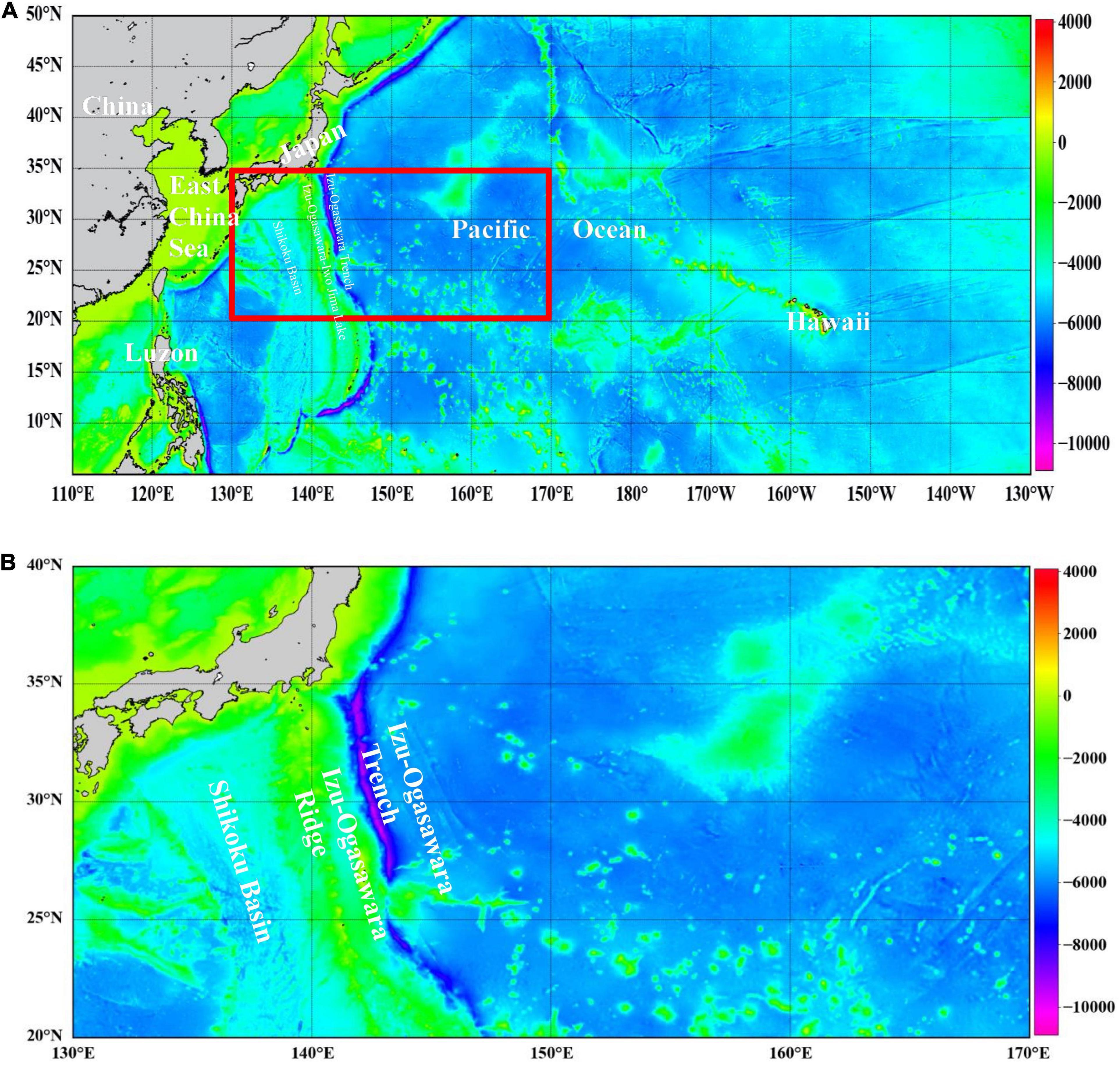
Figure 1. The location and topographic mapping of our study area. (A) Location. (B) Topographic mapping.

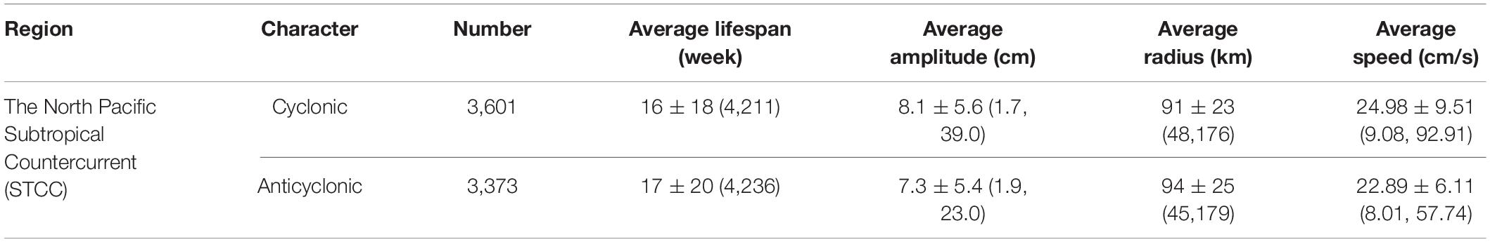
Table 1. Statistics of mesoscale eddies in the STCC from 1993 to 2018.

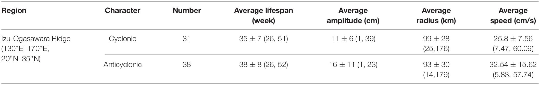
Table 2. Statistics of 69 mesoscale eddies in study from 1993 to 2018.

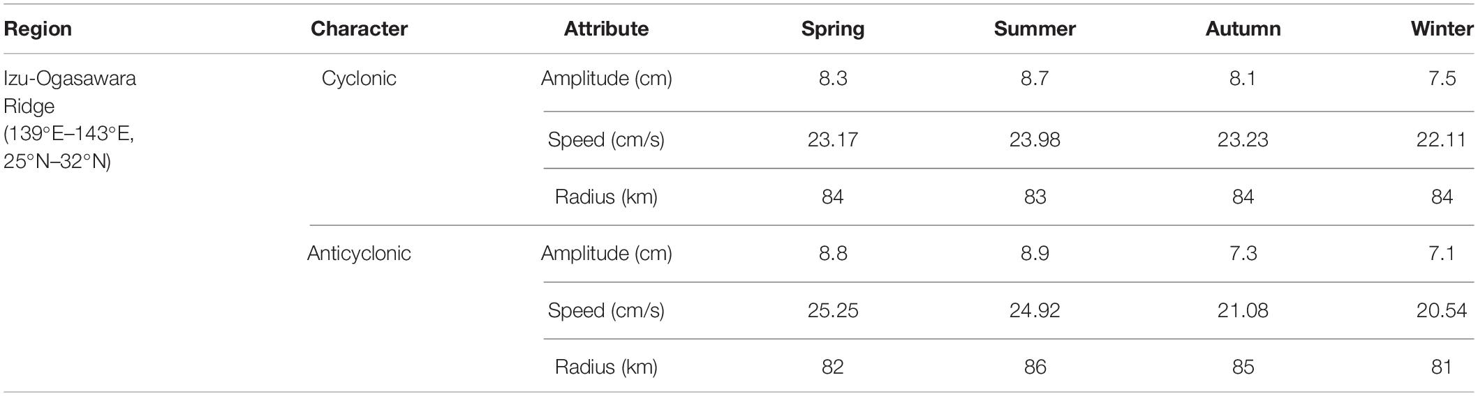
Table 3. Seasonal and polarized statistics of all mesoscale eddies in the ridge region (130°E–170°E, 20°N–35°N) from 1993 to 2018.

The topography of Izu-Ogasawara Ridge has been retrieved from ETOPO1, the global integrated bathymetric-topographic digital elevation model (DEM), to discover the potential topographic effects on mesoscale eddies, with the terrestrial topography and ocean water depth provided, at the highest resolution, as a grid-registered, 1 arc-minute grid that spans from pole to pole and from −180° to 180° in longitude. The Izu-Ogasawara Ridge is located in the northwest of the Philippine Sea, which occupies a large part of the Northwest Pacific, and the Philippine Sea Plate forms its seafloor topography, long from north to south, narrow from north to south, at a large water depth, with a variety of islands, ridges, ocean basins, deep trenches, and other topography. The range of Izu-Ogasawara Ridge starts from Nagoya, Honshu, Japan to the southern area of Tokyo, and the open ocean constitutes the Ogasawara-Iwo Jima arc. Along the eastern side of the ridge runs the Izu-Ogasawara Trench, with the maximum depth deeper than 9,000 m, and to the western of the ridge, there is flat Shikoku Basin, the depth of which ranges approximately from 4,000 to 5,000 m. According to the former studies based on the observational data, the vertical scale of the mesoscale eddies could reach about 1,000 m in the region around the ridge (Zhang et al., 2013). On the other hand, the water depth along the trajectories that 69 mesoscale eddies travel within the ridge has been started from 110 m to more by statistics, and this means that the topography of the ridge could indeed directly influence the attributes of mesoscale eddies during the evolution and propagation process.

Mathematical Statistics and Wavelet Analysis

Initialization

As the origin of mesoscale eddies in our study can be traced back in a variety of starting time, formation location, and successive lifespan intervals, we first uniformly reset the arrival time to the east ridge edge as the reference origin time 0, so that the standard timeline could be consistently imposed on all mesoscale eddies. Let the total number of mesoscale eddies be I, with the i – th mesoscale eddy denoted as M_i(t_i), i = {1, 2, …, I}, where t_i refers to the survival time that the given mesoscale eddy activity moves forward, and the amplitude, rotation speed, radius of the given mesoscale eddy could then be, respectively, defined as A_i(t_i), S_i(t_i), and R_i(t_i). For each mesoscale eddy, we first transform the time domain in the above three indices to identically align the arrival time as follows:

where t_i0 is the time point that the mesoscale eddy originally pass through the ridge, and the transformed $t_{\text{i}}^{{}^{\prime }}$ reset the arrival time with $t_{\text{i}}^{{}^{\prime }}=0$ when the mesoscale eddy the east ridge edge.

Temporal Regularity

After the initialization stage, we make a temporal regularity for all the mesoscale eddies thoroughly proceeding within the ridge region. Let $(x_{\text{i}}(t_i^{{}^{\prime }}),y_{\text{i}}(t_i^{{}^{\prime }}))$ be the longitude and the latitude of the geographical location that each mesoscale eddy moves toward, with r indicating the ridge region. Among all those mesoscale eddies completely passing over the ridge, i.e., for any time $t_{\text{i}}^{{}^{\prime }}\ge 0$ in a given mesoscale eddy, if $(x_{\text{i}}(t_{\text{i}}^{{}^{\prime }}),y_{\text{i}}(t_{\text{i}}^{{}^{\prime }}))\notin r$ exists, we first examine every timespan across the whole ridge region by defining $t_{i\max }^{{}^{\prime }}=t_{\text{ir}}^{{}^{\prime }}$, with $t_{\text{ir}}^{{}^{\prime }}$ representing the time duration when the mesoscale eddy moves to the west edge of the ridge region, and then find out the maximum timespan duration $t_{{}^{*}\max }^{{}^{\prime }}=\underset{\mathrm{i}=1:\mathrm{I}}{argmax}(t_{\text{ir}}^{{}^{\prime }})$, from all the mesoscale eddies that completely move out of the ridge edge. Furthermore, we define a temporal scaling index between the real and the maximum timespan duration $t_{{}^{*}\max }^{{}^{\prime }}$ across the ridge, with the interval from the arrival to departure time toward the ridge, and then align and extend each mesoscale eddy trajectory to be considered to an equal timespan length via interpolation.

For example, for the amplitude time series of each given mesoscale eddy that completely goes across the ridge, $A_{\text{i}}(t_{\text{i}}^{{}^{\prime }})$, $t_{\text{i}}^{{}^{\prime }}\in [0,t_{\text{ir}}^{{}^{\prime }}]$, the cubic spline interpolation has been applied for the newly updated one $A_{\text{i}}^{{}^{\prime }}(t_{\text{i}}^{{}^{\prime }})$ with the assumed form of the cubic polynomial curves to fit for each segment,

where J refers to the number of the segments in total, j stands for the j-th segment, and α, β, γ are respectively the coefficients of the polynomial curves, λ is a constant term, O represents the result of fitting, and the spacing of the amplitudes between the successive time points is:

The interpolation of cubic spline constrains the function itself, as well as the first derivative and the second derivative, so the routine must ensure that $O_{\text{i}}\left(A_{\text{i}}(t_{\text{i}}^{{}^{\prime }})\right)$, $O_{\text{i}}^{{}^{\prime }}\left(A_{\text{i}}(t_{\text{i}}^{{}^{\prime }})\right)$, and $O_{\text{i}}^{{}^{\prime }{}^{\prime }}\left(A_{\text{i}}(t_i^{{}^{\prime }})\right)$ are equal at the interior node points for adjacent segments. We substitute the coefficients by the new variable s for the polynomial’s second derivative in each segment for simplification. For the j – th segment, the governing equation is,

In matrix form, the governing equation could be reduced to a tri-diagonal form.

where s₁ and s_J are zero for the natural spline boundary condition. In this way, the polynomial definition for each segment could be deduced as follows:

Spatial Normalization

We further make a spatial normalization for those mesoscale eddies that partially travel the ridge, i.e., for any time $t_{\text{i}}^{{}^{\prime }}\ge 0$, if all the geographical locations range within the ridge, $(x_{\text{i}}(t_{\text{i}}^{{}^{\prime }}),y_{\text{i}}(t_{\text{i}}^{{}^{\prime }}))\in r$, which means the mesoscale eddy does not completely go across the edge of the ridge region. Given the standard spatial distance d_max that the mesoscale eddy moves across the ridge with the maximum timespan $t_{{}^{*}\max }^{{}^{\prime }}$, we denote one spatial scaling index between the real distance d and the standard distance d_max, and further modify their time intervals $t_{\text{i max}}^{{}^{\prime }}$ starting from the reference time 0 accordingly, to align the spatial distance for each given mesoscale eddy as follows,

where $t_{\text{i max}}^{{}^{\prime }}$ could be regulated with the help of the above spatial scaling index, considering the maximum timespan duration over the ridge $t_{{}^{*}\max }^{{}^{\prime }}$, and the corresponding standard distance d_max, i.e., the measurement from the arrival position to the departure position toward the entire region of the ridge. For the real distance d_i and the standard distance d_max, the referred time domain are $t_i^{{}^{\prime }}\in [0,t_{iend}^{{}^{\prime }}]$ and $t_{{}^{*}}^{{}^{\prime }}\in (0,t_{{}^{*}\max }^{{}^{\prime }})$. The cubic spline interpolation would hereby be applied again to normalize the initial amplitude time series $A_{\text{i}}(t_{\text{i}}^{{}^{\prime }})$, $t_{\text{i}}^{{}^{\prime }}\in [0,t_{iend}^{{}^{\prime }}]$, into the newly updated one $A_{\text{i}}^{\prime }(t_{\text{i}}^{\prime })$, for each given mesoscale eddy that partially goes across the ridge.

Range Expansion

At last, we expand the domain of survival time in study to ranges out of the ridge region for all the mesoscale eddies, and follow the scaling principle derived from the ratio between the real and the corrected time duration in the ridge for all the mesoscale eddies completely or partially passing over it, by interpolation. For example, when we try to make the range extension to the time domain [-30, 150] days after resetting the time series at the initialization stage, for the regulated amplitude $A_{\text{i}}^{{}^{\prime }}(t_{\text{i}}^{{}^{\prime }})$ of each given mesoscale eddy that completely goes across the ridge, we could similarly employ temporal regularity strategy by $t_{\text{i}}^{{}^{\prime }}\times 30\mathrm{/}{t}_{{}^{*}\max }^{{}^{\prime }}$ and $t_{\text{i}}^{{}^{\prime }}\times \left(150-t_{{}^{*}\max }^{{}^{\prime }}\right)\mathrm{/}{t}_{{}^{*}\max }^{{}^{\prime }}$ for the time domain before and after travailing into the ridge. For the mesoscale eddies that partially travel the ridge, we only need to extend the temporal regularity by $t_i^{{}^{\prime }}\times 30\mathrm{/}{t}_{i\max }^{{}^{\prime }}$.

Topographic Extraction

We collect the corresponding longitude and latitude along the way that mesoscale eddy trajectories pass, then apply the integrated bathymetric digital elevation of Izu-Ogasawara Ridge from ETOPO1, to discover the potential topographic effects on mesoscale eddies. Let the altitude at the geographical location $(x_{\text{i}}(t_i^{{}^{\prime }}),y_{\text{i}}(t_i^{{}^{\prime }}))$ along the trajectory of each given mesoscale eddy be B_i(t_i). We follow the same principle mentioned above to extract the standardized time series of the amplitude, rotation speed, radius, altitude for the given mesoscale eddy, i.e., $A_{\text{i}}^{{}^{\prime }}(t_{\text{i}}^{{}^{\prime }})$, $S_i^{{}^{\prime }}(t_{\text{i}}^{{}^{\prime }})$, $R_{\text{i}}^{{}^{\prime }}(t_{\text{i}}^{{}^{\prime }})$, and $B_{\text{i}}^{{}^{\prime }}(t_{\text{i}}^{{}^{\prime }})$. We intuitively apply the mathematical statistics to all the mesoscale eddies in study by the aligned time averaging, for the above types of the potentially correlative time series, forming the mean curve of the altitude, the amplitude, rotation speed, radius of all the mesoscale eddy trajectories, E_A(t′), E_S(t′), E_R(t′), and E_B(t′), which sums up into the averaged variation curves to investigate how much of the possible impacts they might response to the topographic effects during the movement of the mesoscale eddies across the ridge.

Standardization

The zero-mean normalization will be further applied to all the above standardized mesoscale eddy trajectories in study with an extension over time, those completely spanning the ridge or those that demise within the ridge in comparison, in terms of the mesoscale eddy amplitude, rotation speed, radius and the altitude.

where μ_A, μ_S, μ_R, and μ_B are respectively the mathematical expectation of E_A(t′), E_S(t′), E_R(t′), E_B(t′), σ_A, σ_S, σ_R, and σ_B are respectively the standard deviation of E_A(t′), E_S(t′), E_R(t′), and E_B(t′). Meanwhile, it is appropriate to identify those samples with the deviation that is highly probable to have an impact on assessment, and hereby to categorize as requiring quality control and eliminating singular values from time series of mesoscale eddy trajectories with and without passage.

Wavelet Coherence

Let Y(t) be the mean curve of topography around the Izu-Ogasawara ridge. The cross-wavelet transform between the intrinsic attributes of the mesoscale eddies X(t) and the topography can be represented as:

where W_X(a, τ) and W_Y(a, τ) are respectively the wavelet transforms of X(t) and Y(t), and ${\overline{W}}_{\text{Y}}(a,\mathrm{\tau })$ indicates the complex conjugation of W_Y(a, τ), a is a scale factor, representing the period length of the wavelet, and τ is a shift factor, reflecting the shift in time. The covariance between the cross-wavelet power spectrum is then defined as follows:

The correlation between the intrinsic attributes of the mesoscale eddies and the topography could be further measured via wavelet coherence (Rhif et al., 2019), as follows:

where s(W_XY(a, τ)) is the cross spectral density between X(t) and Y(t), with a smoothing operator s. The wavelet coherence coefficient reflects the synchronization similarity.

Results

In our simulation experiment, mesoscale eddy trajectories of a life cycle more than 6 months, across the Izu-Ogasawara Ridge from east to west from 1993 to 2018, within the study area (130°E–170°E, 20°N–35°N), have been quantitatively investigated, to explore the potential spatio-temporal correlation with the topographic effects, with the average lifespan 37 weeks, the average amplitude 14 cm, the average radius 96 km, the average rotation speed 29.5 cm/s. Figure 2 displays all the 69 mesoscale eddy trajectories, where 32 of them completely pass through the ridge from east to west, and 37 of them only partially leap over one side of the ridge and then demise inside it, with cyclonic eddies in black and anticyclonic eddies in white.

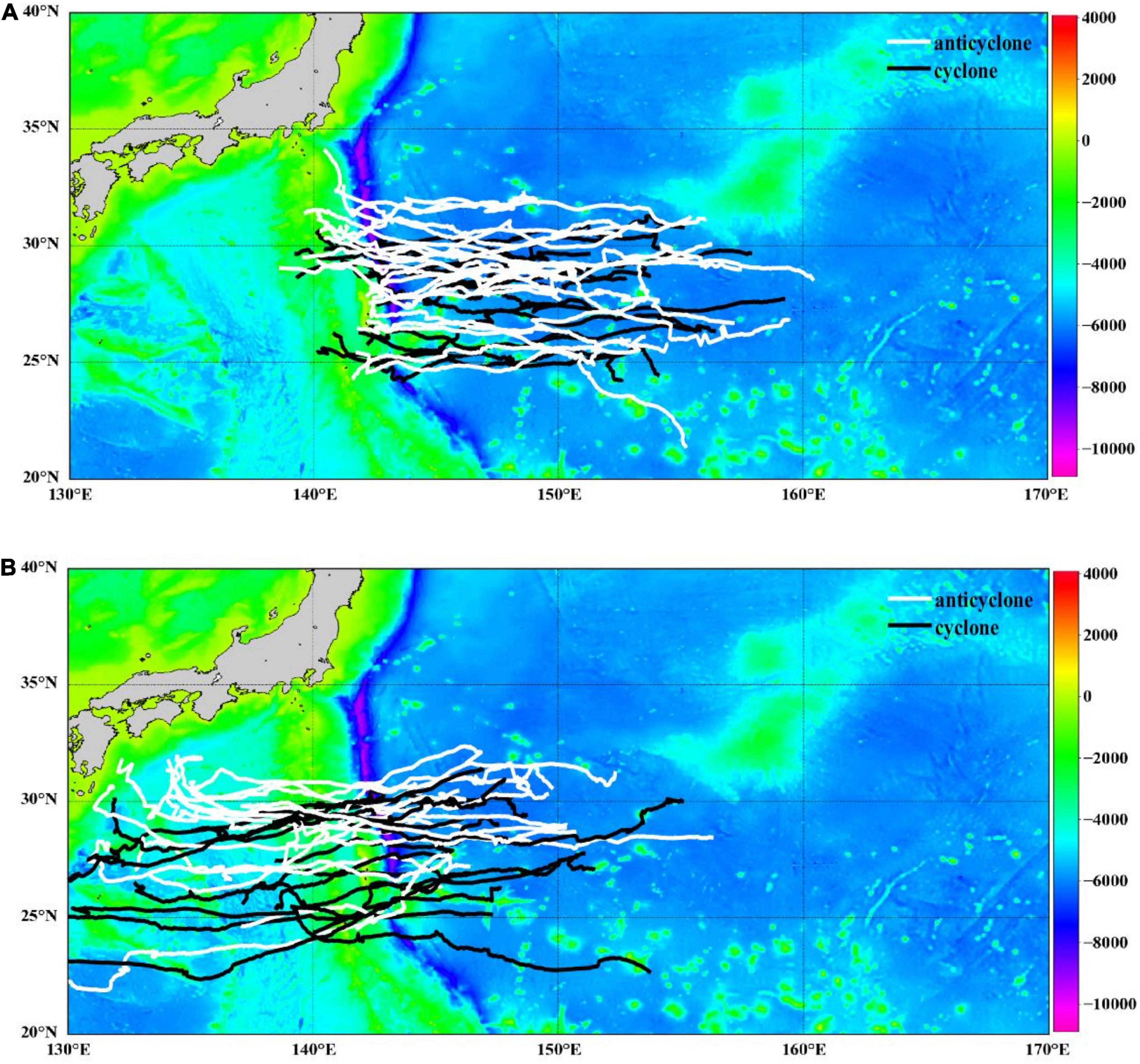
Figure 2. Mesoscale eddy trajectories. (A) Mesoscale eddy trajectories that completely pass through the ridge, with cyclonic in black and anticyclonic in white. (B) Mesoscale eddy trajectories that partially travel across the ridge, with cyclonic in black and anticyclonic in white.

We screened out the solely mesoscale eddy which exhibited the maximum timespan duration within the ridge, 116 days, from all of the 32 mesoscale eddy trajectories that completely go through the ridge, and accordingly retrieved the distance 513.2 km that particular mesoscale eddy moves from the east to the west across the ridge. We standardized time series of the amplitude, rotation speed, radius for all the 32 mesoscale eddies in temporal regularity process.

We conducted the spatial normalization to all the 69 mesoscale eddy trajectories, to ensure all the trajectories of the same statistical significance across the aligned maximum timespan duration within the ridge, for not only those completely pass through the ridge but also those partially go across the ridge.

We further extended the time domain in study from [0, 116] to [-30, 150] days, i.e., to consider more the mesoscale eddy activities before and after reaching the edge of the ridge. We carried out the mathematical statistics to explore the potential spatio-temporal correspondence between the topography and the three attributes of mesoscale eddies, i.e., the amplitude, rotation speed, radius, by respectively synthesizing all the individual time series into a timely aligned averaged curve. The time series of the amplitude, rotation speed, radius for all the 69 mesoscale eddies after range extension have been individually illustrated in Figure 3, with the mean curve in red thick lines indicating the tendency as a whole.

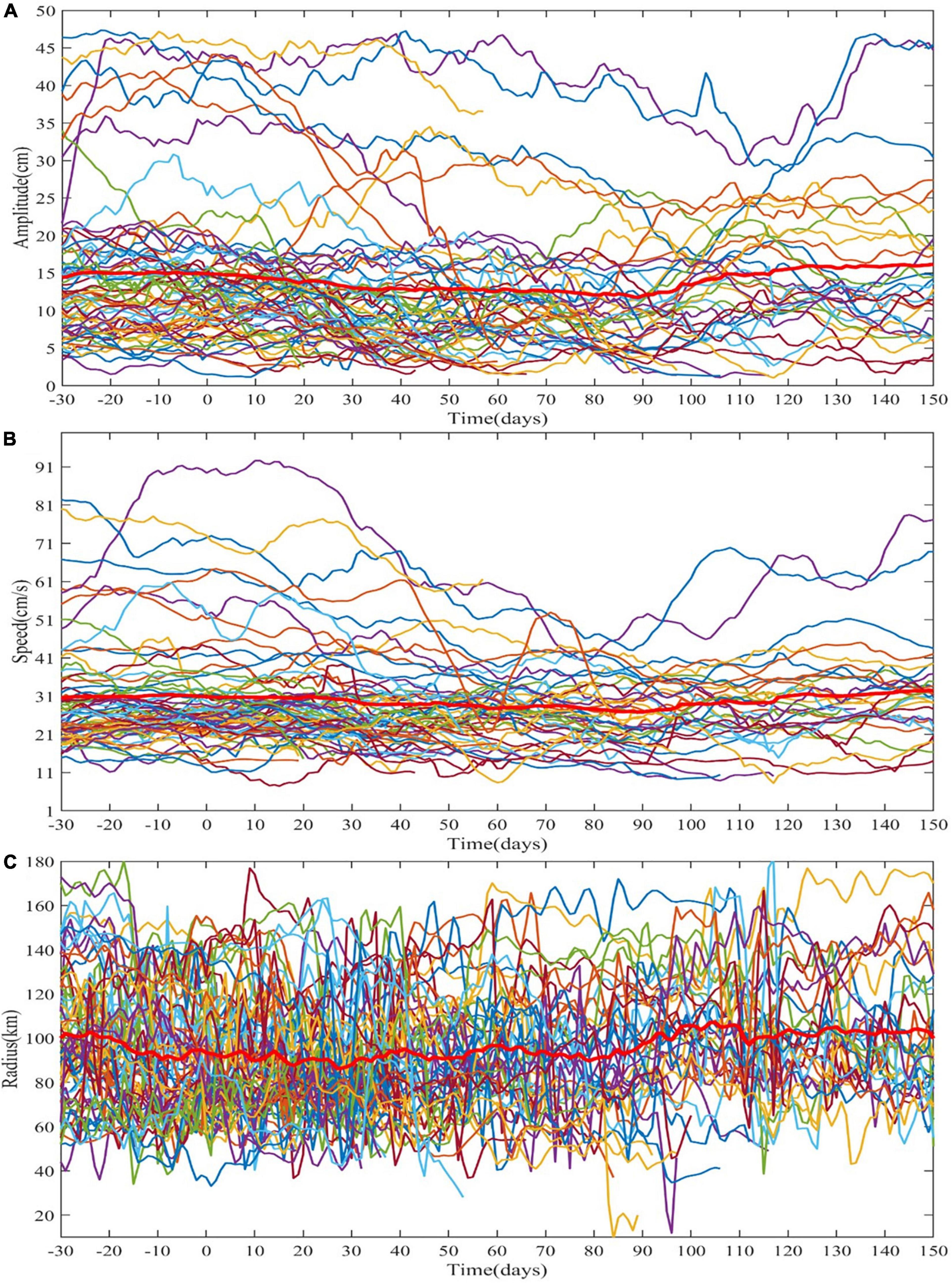
Figure 3. The intrinsic attribute curves of 69 mesoscale eddies. (A) Amplitude curves of 69 mesoscale eddies after spatial normalization. (B) Rotation speed curves of 69 mesoscale eddies after spatial normalization. (C) Radius curves of 69 mesoscale eddies after spatial normalization.

The corresponding mean topography curve are averagely accumulated from the altitude at each geographical location over the ridge along all the mesoscale eddy trajectories referred. We collectively made a comparison between the mean curves of both the topography and three impact factors about the mesoscale eddies, i.e., the amplitude, rotation speed, radius, under the condition whether the mesoscale eddies go across the ridge, as is shown in Figure 4, with all the 69 mesoscale eddy trajectories in black, 32 completely passing in red, 37 partially passing in blue, in the top three rows, respectively, the gray shading indicating the transition before, during, and after the eddy-ridge interaction, and in the last row, the mean altitude has been listed, corresponding the eastward (143°E–146°E, 20°N–35°N), the interior (139°E–143°E, 20°N–35°N), the westward (136°E–139°E, 20°N–35°N) to the ridge. We also particularly plot the mean curves of the topography in black, mesoscale eddy amplitude in blue, radius in cyan, and rotation speed in red together after standardization with quality control, for all the 69 mesoscale eddy trajectories, as well as mesoscale eddy trajectories that completely pass through the ridge and partially travel across the ridge, regarding to the vortex polarity, with the vertical dashed lines indicating the beginning and end time points within the ridge region, as is shown in Figure 5. The zonal and meridional drifting speed have also been statistically observed along the extended range of the time domain daily on average in Figure 6, regarding to the vortex polarity and the passage of the ridge, with the statistics of all the 69 mesoscale eddy trajectories in black, the cyclonic eddies with passage in red, the anticyclonic eddies with passage in blue, the cyclonic eddies without passage in green, the anticyclonic eddies without passage in yellow.

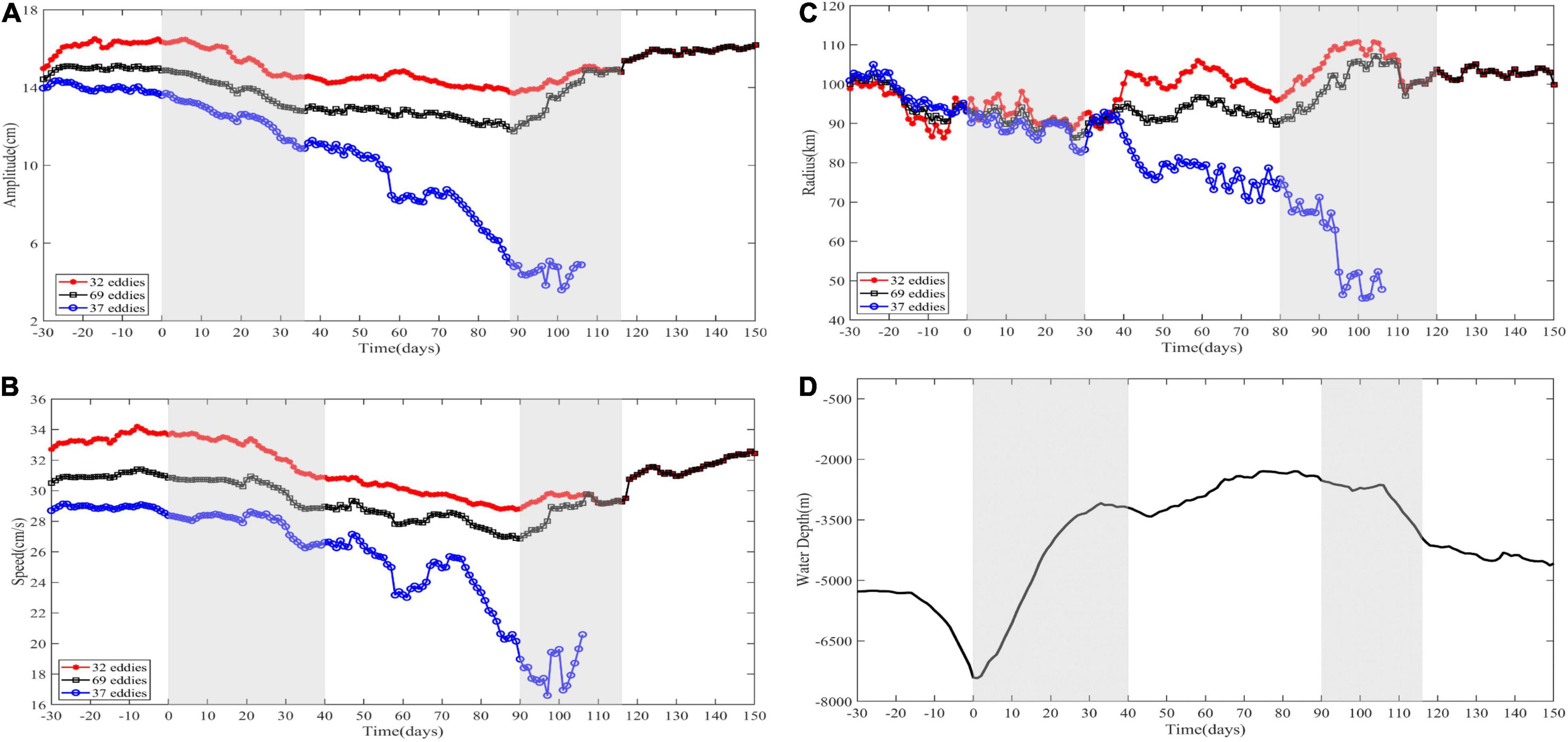
Figure 4. Comparison of mesoscale eddy amplitude, rotation speed, radius with topography under conditions. (A) The mean curve of the amplitude for 69/32/37 mesoscale eddy trajectories. (B) The mean curve of the rotation speed for 69/32/37 mesoscale eddy trajectories. (C) The mean curve of the radius for 69/32/37 mesoscale eddy trajectories. (D) The mean curve of the topography for 69 mesoscale eddy trajectories (136°E–146°E, 20°N–35°N).

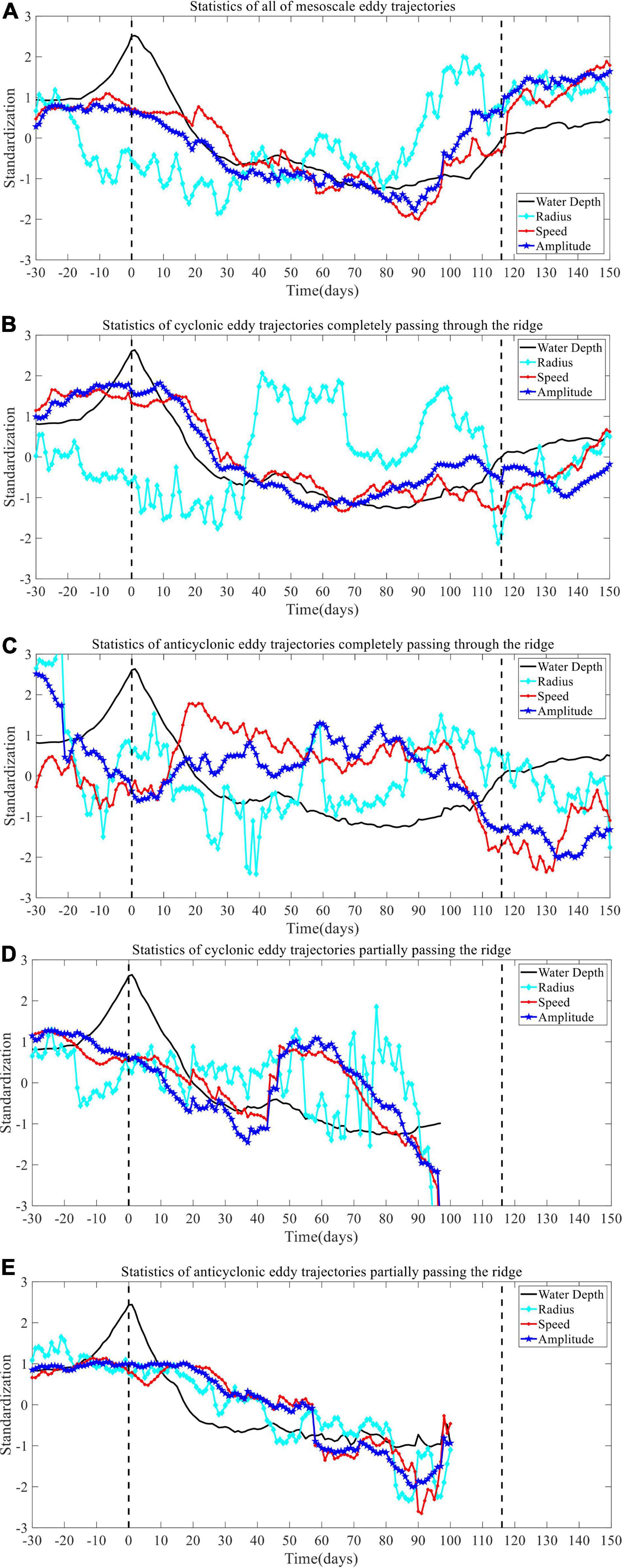
Figure 5. Mean curve mapping of amplitude, rotation speed, radius, and topography after standardization. (A) The statistics in all of 69 mesoscale eddy trajectories. (B) The statistics in cyclonic eddy trajectories that completely pass through the ridge. (C) The statistics in anticyclonic eddy trajectories that completely pass through the ridge. (D) The statistics in cyclonic eddy trajectories that partially pass the ridge. (E) The statistics in anticyclonic eddy trajectories that partially pass the ridge.

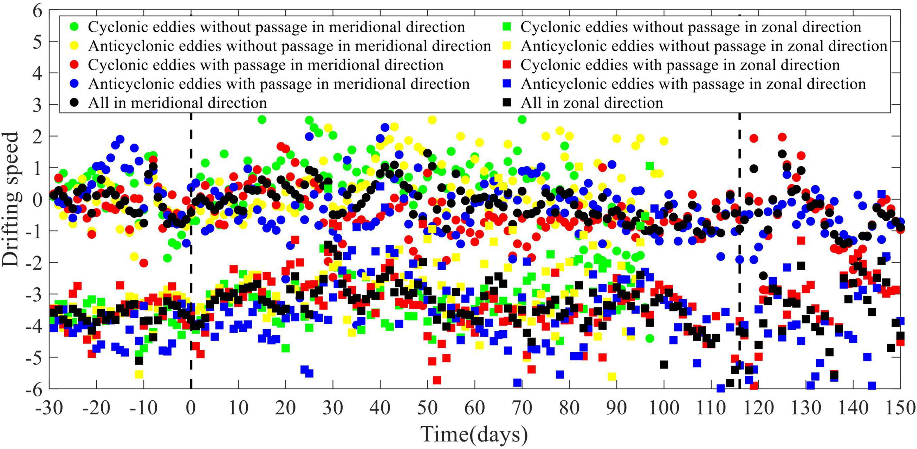
Figure 6. Distribution of zonal and meridional drifting speed.

We utilized the wavelet coherence to search for how frequently and how much extent the topography effects could exert possible impact to the variation in mesoscale eddy trajectories over time, in terms of the three relevant indices, i.e., the amplitude, rotation speed, radius, and described the lead-lag effects through the wavelet phase difference. The wavelet coherence map between the mean altitude and the average amplitude, rotation speed, radius of mesoscale eddy trajectories over time are respectively shown in Figure 6, where wavelet correlation is affected by discontinuity, and the color bar corresponds to the relative intensity of each frequency. The stronger correlation tends to be in red, while weaker correlation in blue, from red to blue, the coherence spectrum values decrease in order. The cone of influence (COI), the region of the wavelet spectrum with edge effect, is denoted in thick black curve. Since the region in COI will be influenced by boundary distortion, reliable information could not be provided and should be removed. And 5 and 10% significance levels are respectively indicated in black thin line and black dashed line, with the significance value generated by Monte Carlo simulation (Aguiar-Conraria and Soares, 2011).

Discussion

In this manuscript, we address to systematically and quantitatively investigate the topographic effects on evolution and propagation of mesoscale eddies across Izu-Ogasawara Ridge in Northwestern Pacific Ocean, in term of three relevant attributes, i.e., the amplitude, rotation speed, radius. We explore the potential topography effects through three phases of life cycle, i.e., before, during, and after the interaction with the ridge, by both the direct observation and the wavelet coherence map, from the perspective of the time-frequency domain. When the mesoscale eddies approach the ridge, and the steepness of the mean topography curve becomes higher, we observed from Figures 5B,D that most of the cyclonic eddies obviously tended to begin to decay or even demise, and the amplitude, rotation speed, radius of the mesoscale eddies decreased until some of the mesoscale eddies could move across the top of the ridge. The mean topography curve dropped, the three relevant attributes gradually increased, consistently coherent with the variation of the topography. On the contrary, it has been illustrated from Figures 5C,E that some of the anticyclonic eddies tended to intensify slightly and some didn’t make a significant difference, regarding to the amplitude, rotation speed, radius, when encountering the upslope of the ridge. The general southwestward or northwestward mesoscale eddy trajectories tended to modify toward a more equatorward direction or oppositely by forcing the meridional components, as is shown in Figure 6, which is coherent to the previous studies (Beismann et al., 1999).

For topography vs. mesoscale eddy amplitude, it has been implied from the experimental results in Figures 4A,D, 5A–E that there has been generally significant correlation between the two time series within the ridge region on the whole (139°E–143°E, 20°N–35°N). The mean amplitude value through life cycle of all 69 mesoscale eddies is 14.1 cm with the standard deviation of 9.5 cm, while the mean amplitude values of all the cyclonic eddies and all the anticyclonic eddies are respectively 11.6, 18.6 cm with passage and 10.4, 10.3 cm without passage over the ridge, implying that the mesoscale eddies that partially travel across the ridge often exhibit a tendency on the verge of demise, with relatively small amplitude values on a whole. The sudden changes with a range over 10% of the mean amplitude value in a 7-day period after standardization and quality control happen on the 92nd–97th days for 69 mesoscale eddies, the 13th–24th days and the 6th–13th, 28th–31st, 38th–46th, 59th–75th, 80th–89th days for cyclonic eddies with and without passage, the −30th to −22nd, 51st–55th, 104th–109th days and the 19th–26th, 52nd–58th, 75th–83rd, 88th–94th days for anticyclonic eddies with and without passage, along the time domain. In the 0–36th days, the mean topography curve gradually rises, with the depth rise from −7,409 to −3,134 m roughly, the mean amplitude curve gradually decreases from 14.3 to 9.5 cm for cyclonic eddies, with a relative decline of 33.6%, while the mean amplitude curve for anticyclonic eddies first rises from 12.7 to 13.6 cm, and then drops till 12.3 cm. To be exactly, the mean amplitude curve of cyclonic eddies falls from 15.6 ± 8.2 to 11.2 ± 5.4 cm with complete passage and from 13.0 ± 5.6 to 7.8 ± 4.9 cm with partial passage, on the contrary, the mean amplitude curve of anticyclonic eddies increases from 11.0 ± 2.5 to 13.4 ± 3.0 cm with complete passage, remains around 14.4 ± 9.8 cm for 21 days and then descends to 11.2 ± 11.1 cm with partial passage. When the mean topographic curve starts the downward trend, and accordingly the mean amplitude curve demonstrated the upward growth. Starting from the 88th day, the mean altitude value drops from roughly −2,410 to −3,792 m, and the corresponding mean amplitude has been recovered from 9.0 to 12.1 cm for cyclonic eddies, and from 7.9 to 9.0 cm for anticyclonic eddies. To be exactly, the mean amplitude curve of cyclonic eddies rises from 10.6 ± 4.9 to 12.1 ± 4.3 cm with complete passage over ridge, drops from 7.4 ± 3.7 to 1.4 ± 0 cm till the demise with no passage, in contrast, the mean amplitude curve of anticyclonic eddies decreases from 12.9 ± 3.0 to 9.0 ± 1.8 cm with complete passage, increases from 3.0 ± 0.9 to 7.0 ± 0 cm till dying with partial passage. After the range extension, it is found that around the region eastward to the ridge edge (143°E–146°E, 20°N–35°N), there tended to be a more stable variation of the mesoscale eddies, compared to that across the ridge region, with the average amplitude 14.8 cm for cyclonic eddies, and 14.0 cm for anticyclonic eddies. It seemed that no obvious evidence could be shown for the topography effects outside the east edge of the ridge. While the region westward to the ridge edge (136°E–139°E, 20°N–35°N) still involves the topography variation from roughly −3,954 to −4,583 m, the mean amplitude grew from 10.8 to 11.7 cm for cyclonic eddies, with an relative increase of 8.7%, and the mean amplitude decreased from 9.1 to 9.0 cm for anticyclonic eddies, with an relative drop of 1.1%. It has also been shown from the wavelet coherence map in Figure 7A that in the short-term frequency band of 2–5 days, the significantly strong correlation occurred on the 15–25th days and the 93–110th days, when the mesoscale eddies just reached the east edge of the ridge or approached to leave away from the ridge region. In the medium-term frequency band of 7–10 days, there has been significant correlation reflected on the 30–50th days. From the long-term frequency band of 16–25 days, the strong correlation lasted during the 80–110th days when the mesoscale eddies almost arrived at the west edge of the ridge.

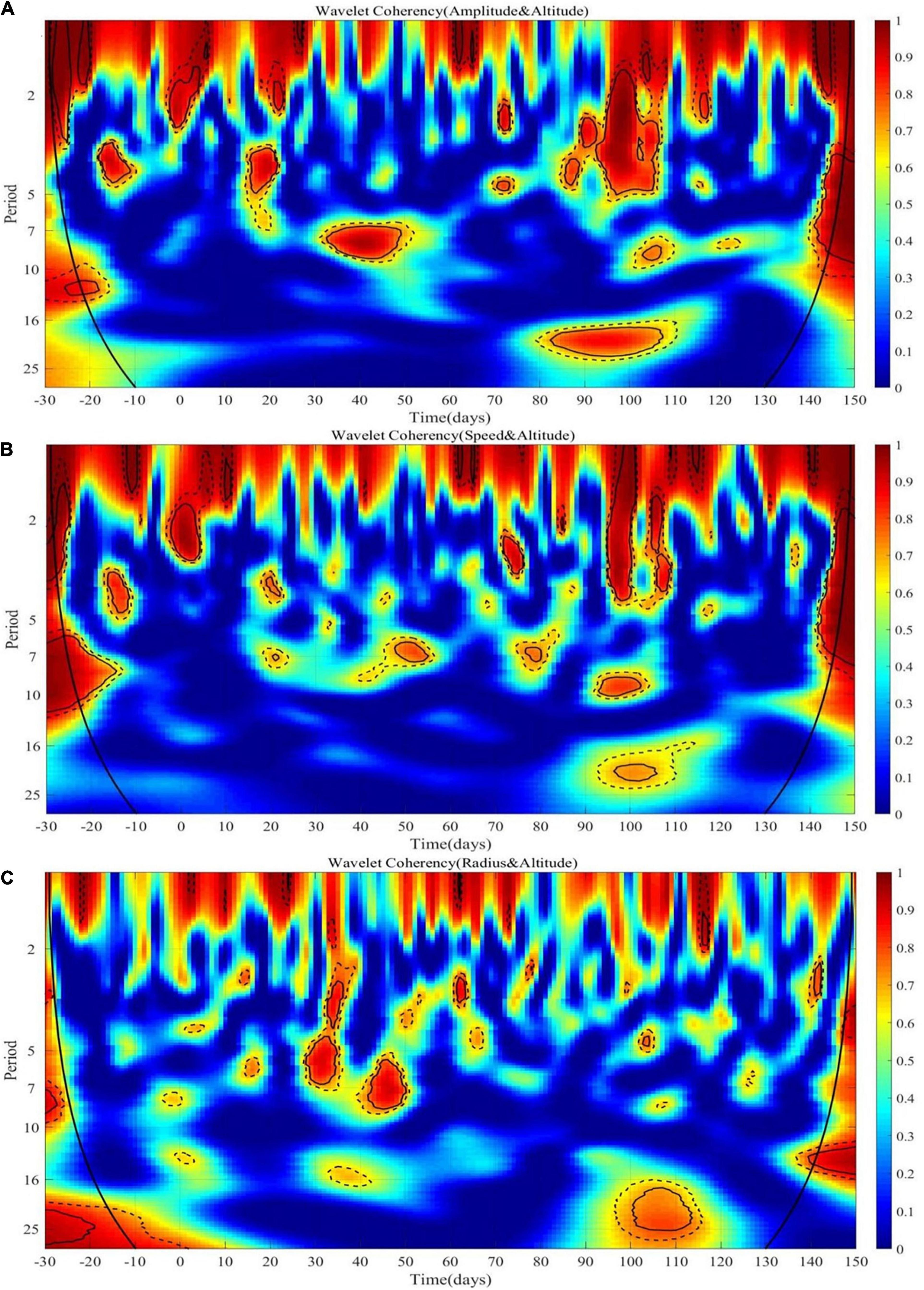
Figure 7. Wavelet coherence mapping. (A) Wavelet coherence map between mesoscale eddy amplitude and topography. (B) Wavelet coherence map between rotation speed of mesoscale eddy and topography. (C) Wavelet coherence map between mesoscale eddy radius and topography.

For topography vs. rotation speed of mesoscale eddies, it has been demonstrated from the experimental results in Figures 4B,D, 5A–E that around the region eastward to the ridge edge (143°E–146°E, 20°N–35°N), both the mean topography curve and the mean rotation speed behaved relatively stable for all of 69 mesoscale eddies, with the altitude value −5,279 and the rotation speed 31.0 cm/s. There have been no obvious evidences of the topography effects on the variation of the rotation speed before reaching the ridge. Within the region westward to the ridge edge (136°E–139°E, 20°N–35°N), the rotation speed for all of 69 mesoscale eddies increased from 29.3 to 32.4 cm/s on the whole, with a relative increase of 10.6%. However, it has been seen within the ridge region (139°E–143°E, 20°N–35°N) after standardization and quality control, in the 0–40th days, the mean rotation speed gradually decreases from 28.9 to 24.9 cm/s for cyclonic eddies with a relative reduction of 13.8%, and the mean rotation speed increases from 27.8 to 28.1 cm/s for anticyclonic eddies with a relative rise of 1.1%, when the mean topography curve gradually rises. To be exactly, the mean rotation speed curve of cyclonic eddies drops from 30.3 ± 10.7 to 26.3 ± 8.6 cm/s with complete passage and from 27.5 ± 6.9 to 23.5 ± 9.3 cm/s with partial passage, conversely, the mean rotation speed curve of anticyclonic eddies first grows from 25.9 ± 1.5 to 30.6 ± 0.7 cm/s and then decreases to 28.9 ± 3.6 cm/s with complete passage, and first descends from 29.8 ± 14.2 to 28.5 ± 12.8 cm/s, rises to 30.7 ± 14.9 cm/s, and finally drops to 27.2 ± 12.3 cm/s with partial passage. Around the 90th day, when the altitude value is −2,427 m, the rotation speed decreases and reaches to the minimum 23.3 cm/s for cyclonic eddies, and gets to 22.0 cm/s for anticyclonic eddies, where the rotation speed values are respectively 25.4 ± 7.8, 28.1 ± 4.8 cm/s with passage and 21.2 ± 8.7, 16.0 ± 2.5 cm/s without passage over the ridge. In the 90–116th days, when the mean topographic curve drops from roughly −2,427 to −3,793 m, and the rotation speed gradually returned to 24.9 cm/s for cyclonic eddies, to 22.8 cm/s for anticyclonic eddies. To be exactly, the mean rotation speed curve of cyclonic eddies increases from 25.4 ± 7.8 to 26.7 ± 7.8 cm/s and then drops to 24.9 ± 7.9 cm/s with complete passage over ridge, falls from 21.2 ± 8.7 to 9.7 ± 0 cm/s till the demise with no passage, on the other hand, the mean rotation speed curve of anticyclonic eddies decreases from 28.1 ± 4.8 to 22.8 ± 0.5 cm/s with complete passage, increases from 16.0 ± 2.5 to 24.7 ± 0 cm/s till dying with partial passage. The mean rotation speed value through life cycle of all 69 mesoscale eddies is 29.8 cm/s with the standard deviation of 12.2 cm/s, while the mean rotation speed values of all the cyclonic eddies and all the anticyclonic eddies are respectively 27.1, 35.4 cm/s with passage and 25.6, 25.7 cm/s without passage over the ridge, implying that the mesoscale eddies that tend to approach dying over ridge mostly have smaller rotation speed values. Although we did not find out the dramatic conversions with a range over 10% of the mean rotation speed value in a 7-day period on the mean rotation speed curve for all 69 mesoscale eddies and cyclonic eddies with passage, they did appear on the 38th–43rd day for cyclonic eddies without passage, the 8th–13th day and the 52nd–57th, 84th–94th day for anticyclonic eddies with and without passage, along the time domain. The coherence between the topography and the rotation speed could be derived. It could also be seen from the wavelet coherence map in Figure 7B that in the short-term frequency band of 2–4 days, there have been significant correlation implied on the 0–10th days and the 95–105th days, when the mesoscale eddies first moved toward the east edge of the ridge and almost exceeded the west edge of the ridge. In the medium-term frequency band of 6–10 days, the strong correlation ranged between the 45–55th and 90–105th days.

For topography vs. mesoscale eddy radius, it has been shown from the experimental results in Figure 4C,D, 5A–E that to the eastern side of the ridge (143°E–146°E, 20°N–35°N), the mean radius curve exhibited a downward tendency for all of 69 mesoscale eddies on the whole, from 100.0 to 93.4 km, with a relative reduction of 6.6%, when the mean topography remains stable to about −5,279 m. Out of the western side of the ridge (136°E–139°E, 20°N–35°N), the mean radius curve was relatively stable on the whole for all of 69 mesoscale eddies, between 100.0 and 105.1 km, when the mean topography curve actually drops from −3,646 to −4,582 m. Therefore, there was no direct evidence of the mutual coherence between the topography and the radius of mesoscale eddies outside the ridge. It has been seen within the ridge region (139°E–143°E, 20°N–35°N) after standardization and quality control, in the 0–30th days, the mean radius for cyclonic eddies first rises from 93.7 to 96.5 km, and then drops till 93.1 km, and the mean radius for anticyclonic eddies first decreases from 107.1 to 81.4 km, and then increases to 93.9 km, when the mean topography curve rises from −7,109 to −3,140 m. To be exactly, the mean radius curve of cyclonic eddies declines from 97.2 ± 17.6 to 88.1 ± 27.1 km and goes up to 95.3 ± 25.9 km with complete passage, and from 90.1 ± 19.9 km down to 82.6 ± 18.6 km and up to 91.0 ± 14.0 km with partial passage, whereas the mean radius curve of anticyclonic eddies grows from 120.0 ± 39.0 to 135.4 ± 19.4 km, drops to 80.9 ± 10.4 km, and recovers to 105.8 ± 35.0 km with complete passage, and descends from 94.2 ± 27.8 to 81.9 ± 20.8 km during a vibration process with partial passage over the ridge. In the 80–100th days, when the mean topography curve is about to decline, the mean radius curve begins to demonstrate an upward tendency for cyclonic eddies, from 98.4 km to nearly 113.5 km, with a relative increase of 15.3%, and from 88.6 km to nearly 94.7 km for anticyclonic eddies. To be exactly, the mean radius curve of cyclonic eddies climbs from 99.9 ± 23.0 to 113.5 ± 14.1 km with complete passage over ridge, dives from 96.8 ± 8.9 to 46 ± 0 km till the demise with no passage, meantime, the mean radius curve of anticyclonic eddies also surges from 102.4 ± 27.0 to 134.9 ± 16.1 km and then decays to 124.4 ± 18.4 km with complete passage, sinks from 74.8 ± 16.0 to 45.7 ± 23.5 km till dying at 65.0 ± 0 km with partial passage. In the 100–120th days, when the topography curve drops from about −2,751 m to about −4,147 m, the mean radius curve of cyclonic eddies declines from 113.5 ± 14.1 to 85.2 ± 25.5 km and then goes up to 95.3 ± 18.2 km with complete passage, while the mean radius curve of anticyclonic eddies descends from 124.4 ± 18.4 to 122.1 ± 17.6 km, rises to 128.4 ± 23.8 km, and drops to 106.3 ± 33.2 km in a repeatedly vibration process with complete passage over the ridge. Unlike the other two relevant attributes, there has been no obviously significant correlation directly from the eddy-ridge interaction on mesoscale eddy radius, but more implications on whether the mesoscale eddies could long survive tend to be revealed from its variation. The mean radius value through life cycle of all 69 mesoscale eddies is 96.4 km with the standard deviation of 27.4 km, while the mean radius values of all the cyclonic eddies and all the anticyclonic eddies are respectively 100.3, 98.2 km with passage and 84.7, 78.7 km without passage over the ridge, demonstrating that the mesoscale eddies that are only able to partially go over the ridge behave a blink of decay with the relatively small radius values. Although we did not find out the sharp alteration with a range over 10% of the mean radius value in a 7-day period on the mean radius curve for 69 mesoscale eddies, they did emerge on the 32nd–38th, 107th–111th days and the −21st to −17th, 84th–91st days for cyclonic eddies with and without passage, the −27th to −18th, −10th to −6th, 6th–11th, 18th–27th, 47th–59th days, and the 38th–43rd, 48th–52nd, and 77th–92nd days for anticyclonic eddies with and without passage, along the time domain. It has also been illustrated from the wavelet coherence map in Figure 7C that in the short-term frequency band of 4–7 days, there existed a correlation on the 28–35th days. In the medium-term frequency band of 7–10 days, the correlation was reflected on the 42–50th days. From the long-term frequency band of 16–25 days, the correlation lasted during the 100–115th days when the mesoscale eddies almost departed the west edge of the ridge.

For topography vs. daily drifting speed of mesoscale eddies, it has been indicated from the experimental results in Figure 6 that there exists a generally significant correlation within the ridge region on the whole (139°E–143°E, 20°N–35°N) as well. The mean daily drifting speeds in both the meridional and zonal direction through life cycle of all 69 mesoscale eddies across the ridge are 0.2 km southward and 3.5 km westward, with the meridional drifting speed and the zonal drifting speed, respectively, 0.1, 0.1, 0.5 and 3.7, 3.4, 3.6 km before, during, and after the interaction with the ridge in the three phases of life cycle. To be exactly, the daily meridional drifting speed of the cyclonic eddies averagely rises from 0.2 km southward to 0.5 km southward, then drops to 0.4 km southward with passage, and increases from 0.1 km northward to 0.4 km northward till demise without passage, meanwhile, the daily meridional drifting speed of the anticyclonic eddies averagely switches from 0.4 km northward to 0.4 km southward, then surges to 0.6 km southward with passage, and shifts from 0.2 km southward to 0.5 km northward till demise without passage. Most of the mesoscale eddies proceeding toward northward disappear on the top of the ridge while those marching to southward mostly tend to survive over the ridge. Almost all of the mesoscale eddy trajectories has a tendency with the increased meridional drifting speeds when reaching the upslope of the ridge. The daily zonal drifting speed of the cyclonic eddies oriented to westward averagely declines from 3.6 to 3.4 km, then down to 3.3 km with passage, and decreases from 3.8 to 3.1 km till decease without passage, on the other hand, the daily zonal drifting speed of the anticyclonic eddies toward westward averagely descends from 4.4 to 3.7 km, then comes up to 4.3 km with passage, and reduces from 3.6 to 3.0 km till the end without passage. Almost all of the mesoscale eddy trajectories exhibits the decayed zonal drifting speeds when emerging the east edge of the ridge. The westward daily zonal drifting speed of anticyclonic eddies looks slightly higher than that of cyclonic eddies on average, owing to the higher drifting performances in anticyclonic eddies that completely pass across the ridge.

It has been concluded that, as is shown in Figures 4–6, regardless of the amplitude and rotation speed, 37 mesoscale eddies were more prone to be significantly influenced by the topography effects, most of which followed the decline tendency, starting from the arrival location until demise over the ridge. 32 mesoscale eddies that completely pass through the ridge exhibited significant negative correlation with the mean topography curve for cyclonic eddies during the evolution process that began at the east boundary of the ridge and lasted until passing over the ridge, while there occurred a little intensified for some of anticyclonic eddies. In total, it could be demonstrated in Figure 5 that for all the 69 mesoscale eddies, except the radius, there exist a highly degree of agreement among the other three attributes after standardization, which further proves the existence of the topographical effects along the life cycle. The highly significant correlation between the topography and the amplitude of the mesoscale eddies could be particularly identified here. When the mesoscale eddies approach the ridge and the water depth gets shallower, the amplitude of the mesoscale eddies decrease for cyclonic eddies and increase a bit for some of anticyclonic eddies accordingly. Then, when the mesoscale eddies leave the ridge and the water depth increase, the amplitude of the mesoscale eddies recover almost to the level before the encounter. This is consistent with the expectation by PV conservation: The vorticity of the eddy and the area of the water column evolve in a compensational way. The vortex column squeezing will lead to the decreasing of the eddy vorticity for cyclonic eddies, and the stretching leads to intensification, conversely, for anticyclonic eddies. The coherence between the mesoscale eddies and the topography impairs the initial stability of the mesoscale eddy structure. This is due to the westward shift of the eddy by the planetary β effect which causes rising up to the shallower region over the eastern slope of the ridge. Namely, as the mesoscale eddies shift to a shallower region, the large frictional spin-down, which is inversely proportional to the lower layer thickness, and the generation of negative vorticity by the conservation of the potential vorticity are carried out. These two phenomena would weaken the eddy structure. Conversely, the westward shift of the cyclonic eddies has a small influence from the topographic effect of the bottom slope. Almost all of the mesoscale eddy trajectories manifests the rise in the daily meridional drifting speed and the decline in the daily zonal drifting speed, at the moment originally outstretching the ridge, no matter with the passage or not. In addition, out of 69 mesoscale eddies, only 32 of them could manage to go across the ridge. It has been revealed from our experimental results that the average horizontal scale of 32 mesoscale eddies that completely pass over the ridge tended to exhibit a relatively large radius on the whole, compared to 37 mesoscale eddies that only partially pass the ridge, whereas 32 mesoscale eddies that completely move across the ridge provided visually dominant clues on both the amplitude and the rotation speed as well, showing the attribute divergence between the mesoscale eddies with passage and without passage over the ridge. We did see from the evaluation of the daily meridional drifting speed that the mesoscale eddies oriented to southward were more likely to survive over the ridge when proceeding toward the upslope of the ridge. It has been reported that the baroclinic or barotropic structure of mesoscale eddies could provide some explanation in the passage or not over the meridian ridge (Kamenkovich et al., 1996). We expect to extend our current work to involve more evidences on the vertical structure of mesoscale eddies over the meridional ridge in the future.

The above potential spatio-temporal dependency could quantitatively reveal how the relevant attributes of mesoscale eddies response to the topography variability over the Izu-Ogasawara Ridge, and inspire to identify the fundamental roles that possible dominantly correlative with the time-varying evolution process. Concerning the self-correlated properties inherently underlined in the propagation of mesoscale eddies, together with the time-frequency interaction imposed from the topography variability, we wish to make an initial attempt to capture the potentially patterns that mesoscale eddy trajectories might dynamically vary during the evolution process over the meridional ridge in the future, via deep learning, such as Long Short Term Memory (LSTM) architecture. Inspired by the real observation statistics in our research, the intrinsic and extrinsic attributes, such as the amplitude, rotation speed, radius, as well as the latitude and longitude at the geographical location, the zonal displacement and meridional displacement, the drifting velocity, and the variation of the bathymetric topography, could engage in deep learning selectively as the multivariate input for the predictive model, which allows to capture and retain long-term dependencies for the variation of mesoscale eddy trajectories, and meanwhile concludes the dominantly mutual linkage between the historic and current mesoscale eddy trajectories. The evaluation on whether and when the topographic attribute involves as input could substantially benefit for the prediction accuracy, will be further comprehensively estimated, when we try to intentionally feed with the topography variation as the additional inputs, rather than only the relevant indices of the amplitude, rotation speed, radius, drifting velocity, supposing the topography effects play relatively leading roles in determining the evolution and propagation of mesoscale eddy trajectories to be predicted.

The life cycle of ocean mesoscale eddies, including generation, decay, dissipation processes, is of great scientific value in understanding the propagation and evolution characteristics. Previous numerical experiments, carried out on the f-plane (Herbette et al., 2003), and on the β-plane (Herbette et al., 2005), with a seamount located in the bottom layers, below the isopycnes in which the surface eddy core resides, showed that surface eddies could get strongly eroded by deformation effects induced by bottom eddies, generated near the topography. Large intense eddies, known to have a long life time on the f-plane, no longer stayed coherent. At the same time, the presence of other poles made the exact path and structure of the eddy, as it impinged on the seamount, hypersensitive to details of the configuration, such as initial eddy position and numerical viscosity. Splitting, and subsequent erosion, of surface eddies became extremely sensitive to the initial conditions.

In contrast to previous studies, the present scheme provides more experimental evidences and hopeful solution with the promise of the end-to-end data-driven modeling of the topographic effects from the real observation data. The survival lifespan, generation date, dissipation date, geographical location, of the mesoscale eddy trajectories are all diverse. The differences of individual mesoscale eddies could easily affect the eddy-ridge interaction evaluation as a whole. So we propose to systematically examine the spatio-temporal dependency from mathematical statistics and wavelet coherence analysis, with the help of temporal regularity, spatial normalization and range expansion, to ensure the understanding of mesoscale eddy trajectories could be identically aligned to the geographical meaning from the standardization perspectives, and to synthesize all the time series statistically, regarding to the polarity. On the premise that all the time series are projected into the same domain, it will be more convenient to carry out the subsequent prediction with sufficient mesoscale eddy samples to be considered for training in deep learning, which could further prove the underlined correlation that the relevant attributes of mesoscale eddies might hold through their life cycle, including the amplitude, rotation speed, radius, and drifting velocity, in combination with the topography effects.

Summary and Conclusion

Ocean mesoscale eddies, involve significant amounts of water movements with irregular, discrete occurrences. Evidences have shown that the variation of mesoscale eddy trajectories would be to some extent attributed to the topographic effects when encountering with mid-ocean ridges, seamounts, bottom slopes, or over a variety of topography, while both the theoretical understanding and the survey from available observational data still remains incomplete. In this manuscript, we propose to make an attempt to explore whether and how the topographic effects of one meridional ridge, could exert considerable influences on the evolution and propagation process of mesoscale eddies through life cycle, directly from the perspectives of real observation statistics. We quantitatively investigate the known variability of ocean mesoscale eddies in the study area (130°E–170°E, 20°N–35°N) from 1993 to 2018, of a life cycle more than 6 months, on the basis of the trajectory atlas retrieved from AVISO satellite altimeter and the integrated bathymetric digital elevation sourced from ETOPO1, including 69 mesoscale eddy trajectories in total, with 32 completely traveling across the ridge, and 37 partially leap over the ridge, to discover the possible eddy-ridge interaction, by both observation statistics and wavelet coherence, with respect to the intrinsic attributes, namely, the amplitude, the rotation speed, the radius. A series of correlative steps, including the initialization, temporal regularity, spatial normalization, range expansion, topographic extraction, wavelet coherence map, have been particularly designed along time-frequency domain to trace back mesoscale eddy trajectories in a variety of origins, location, lifespan, polarity, either completely or partially passing over the ridge, and to facilitate the standardization in statistics across three phases of their life cycle, i.e., before, during and after the interaction with the ridge. It has been revealed in our experiment that three intrinsic attributes of mesoscale eddies within 25 years, all demonstrated significant correlation with the variation of topographic relief over the ridge. The bathymetric topography reflects its relationships with mesoscale eddies through an integrated mode of a short-term, a mid-term, a long-term, respectively in the frequency band with a period of 2–7, 6–10, 16–25 days. We observed that most of the cyclonic eddies obviously tended to begin to decay or even demise, while on the contrary, some of the anticyclonic eddies preferred to intensify slightly, or making no significant difference when encountering the upslope of the ridge until climbing across the top, basically consistent with the expectation of potential vorticity (PV) conservation. The drifting velocity agreed with the tendency that the direction would be more probably modified toward equatorward or poloidally by forcing to the meridional component, with the zonal component reduced at the beginning. The mesoscale eddies with the passage over the ridge exhibited the relatively high average horizontal scales, as well as the relatively high average amplitude and rotation speed on the whole, compared to those with only partially passage. We expect to identify the relevant attributes dominantly correlative with the time-varying evolution process of mesoscale eddies during the eddy-ridge interaction, employ a deep learning architecture, to capture the predictability of mesoscale eddy trajectories on a global scale, when selectively feed the amplitude, rotation speed, radius, the latitude and longitude at the geographical location, the zonal displacement and meridional displacement, the drifting velocity, the variation of the bathymetric topography as the input variables for training. The developed scheme could integrate more evidences on how mesoscale eddies response to the topographic effects during their evolution and propagation process, and help provide opportunities to potentially identify the underlying dynamic patterns and mechanism that mesoscale eddies engage in ocean dynamics with the promise of the end-to-end data-driven solution.

Data Availability Statement

AVISO satellite altimeter database can be available in the AVISO website (https://www.aviso.altimetry.fr/en/data.html). ETOPO1 database is available from NOAA website (http://www.ngdc.noaa.gov/mgg/global/).

Author Contributions

RN has brought up the design of the study, together with analysis and interpretation of data, drafted the manuscript, and made final consent about the manuscript to be published. XG has performed the main experimental work, the analysis and interpretation of data, and drafted the manuscript. ZZ has brought up the conception of the study, provided guidance on data analysis and interpretation. MY, ZF, HX, and HY helped to draft the manuscript. QL helped the analysis and drafted the manuscript. HH and QY helped the statistics. CS has helped with the design and the experiments. LZ has assisted in the experimental work. BH has discussed and helped the experiments. All authors contributed to the article and approved the submitted version.

Funding

This work was supported by the National Key R&D Program (2019YFC1408304), the Natural Science Foundation of People’s Republic of China (42022041), the Natural Science Foundation of People’s Republic of China (41876001), the National Key R&D Program (2016YFC0301400), the National High-Tech R&D 863 Program (2014AA093410), the Natural Science Foundation of People’s Republic of China (31202036), the National Program of International S&T Cooperation (2015DFG32180), the National Science and Technology Pillar Program (2012BAD28B05), and the Natural Science Foundation of People’s Republic of China (41376140).

Conflict of Interest

XG was employed by the company JD.com, Inc.

The remaining authors declare that the research was conducted in the absence of any commercial or financial relationships that could be construed as a potential conflict of interest.

Publisher’s Note

All claims expressed in this article are solely those of the authors and do not necessarily represent those of their affiliated organizations, or those of the publisher, the editors and the reviewers. Any product that may be evaluated in this article, or claim that may be made by its manufacturer, is not guaranteed or endorsed by the publisher.

Acknowledgments

We would like to acknowledge the team members: Yu Cai for his guidance in data analysis.

References

Adduce, C., and Cenedese, C. (2004). An experimental study of a mesoscale vortex colliding with topography of geometry in a rotating fluid. J. Mar. Res. 62, 611–638. doi: 10.1357/0022240042387583
Aguiar-Conraria, L., and Soares, M. J. (2011). Oil and the macroeconomy: using wavelets to analyze old issues. Empir. Econ. 40, 645–655. doi: 10.1007/s00181-010-0371-x
Beismann, J.-O., Käse, R. H., and Lutjeharms, J. R. E. (1999). On the influence of submarine ridges on translation and stability of Agulhas rings. J. Geophys. Res. 104, 7897–7906. doi: 10.1029/1998JC900127
Box, G. E. P., Jenkins, G. M., Reinsel, G. C., and Ljung, G. M. (2015). Time Series Analysis: Forecasting and Control. Hoboken, NJ: John Wiley and Sons. doi: 10.2307/3008255
Braakmann-Folgmann, A., Roscher, R., Wenzel, S., Uebbing, B., and Kusche, J. (2017). Sea level anomaly prediction using recurrent neural networks. arXiv [Preprint]. arXiv:1710.07099
Chelton, D. B., Gaube, P., Schlax, M. G., Early, J. J., and Samelson, R. M. (2011). The influence of nonlinear mesoscale eddies on near-surface oceanic chlorophyll. Science 334, 328–332. doi: 10.1126/science.1208897
Daubechies, I. (1991). Ten Lectures on Wavelets, CBMS-NSF Series in Applied Mathematics. Philadelphia, PA: SIAM. doi: 10.1137/1.9781611970104
Ebuchi, N., and Hanawa, K. (2001). Trajectory of Mesoscale eddies in the Kuroshio recirculation region. J. Oceanogr. 57, 471–480. doi: 10.1023/A:1021293822277
Elman, J. L. (1990). Finding structure in time. Cogn. Sci. 14, 179–211. doi: 10.1016/0364-0213(90)90002-E
Falcini, F., and Salusti, E. (2015). Friction and mixing effects on potential vorticity for bottom current crossing a marine strait: an application to the Sicily Channel (central Mediterranean Sea). Ocean Sci. 11, 391–403. doi: 10.5194/os-11-391-2015
Freedman, D. A. (1981). Bootstrapping regression models. Ann. Stat. 9, 1218–1228. doi: 10.1214/aos/1176345638
Frenger, I., Gruber, N., Knutti, R., and Münnich, M. (2013). Imprint of Southern Ocean eddies on winds, clouds and rainfall. Nat. Geosci. 6, 608–612. doi: 10.1038/ngeo1863
Gangopadhyay, T., Tan, S. Y., Jiang, Z., Meng, R., and Sarkar, S. (2021). “Spatiotemporal attention for multivariate time series prediction and interpretation,” in Proceedings of the IEEE International Conference on Acoustics, Speech and Signal Processing (ICASSP), (Piscataway, NJ: IEEE), 3560–3564. doi: 10.1109/ICASSP39728.2021.9413914
Geurts, P., Ernst, D., and Wehenkel, L. (2006). Extremely randomized trees. Mach. Learn. 63, 3–42. doi: 10.1007/s10994-006-6226-1
Goodfellow, I., Pouget-Abadie, J., Mirza, M., Xu, B., Warde-Farley, D., Ozair, S., et al. (2014). “Generative adversarial nets,” in Proceedings of the Advances in Neural Information Processing Systems (NIPS), (Red Hook, NY: Curran Associates, Inc), 2672–2680. doi: 10.1145/3422622
Greff, K., Srivastava, R. K., Koutník, J., Steunebrink, B. R., and Schmidhuber, J. (2016). LSTM: a search space odyssey. IEEE Trans. Neural Netw. Learn. Syst. 28, 2222–2232. doi: 10.1109/TNNLS.2016.2582924
He, K., Zhang, X., Ren, S., and Sun, J. (2016). “Deep residual learning for image recognition,” in Proceedings of the IEEE Conference on Computer Vision and Pattern Recognition, (Piscataway, NJ: IEEE), 770–778. doi: 10.1109/CVPR.2016.90
Herbette, S., Morel, Y., and Arhan, M. (2003). Erosion of a surface vortex by a seamount. J. Phys. Oceanogr. 33, 1664–1679. doi: 10.1175/2382.1
Herbette, S., Morel, Y., and Arhan, M. (2005). Erosion of a surface vortex by a seamount on the β plane. J. Phys. Oceanogr. 35, 2012–2030. doi: 10.1175/JPO2809.1
Hinton, G. E., and Salakhutdinov, R. R. (2006). Reducing the dimensionality of data with neural networks. Science 313, 504–507. doi: 10.1126/science.1127647
Hochreiter, S., and Schmidhuber, J. (1997). “LSTM can solve hard long time lag problems,” in Advances in Neural Information Processing Systems, eds M. C. Mozer, M. I. Jordan, and T. Petsche (Cambridge, MA: MIT Press), 473–479. doi: 10.5555/2998981.2999048
Hu, J., and Zheng, W. (2020). Multistage attention network for multivariate time series prediction. Neurocomputing 383, 122–137. doi: 10.1016/j.neucom.2019.11.060
Hu, J., Zheng, Q., Sun, Z., and Tai, C. K. (2012). Penetration of nonlinear Rossby eddies into South China Sea evidenced by cruise data. J. Geophys. Res. Ocean 117:C03010. doi: 10.1029/2011JC007525
Huang, G., Liu, Z., Van Der Maaten, L., and Weinberger, K. Q. (2017). “Densely connected convolutional networks,” in Proceedings of the IEEE Conference on Computer Vision and Pattern Recognition, (Piscataway, NJ: IEEE), 4700–4708. doi: 10.1109/CVPR.2017.243
Ihara, C., Kagimoto, T., Masumoto, Y., and Yamagata, T. (2002). Eddy formation near the Izu-Ogasawara Ridge and its link with seasonal adjustment of the subtropical gyre in the Pacific. J. Korean Soc. Oceanogr. 37, 134–143.
Jacob, J. P., Chassignet, E. P., and Dewar, W. K. (2002). Influence of topography on the propagation of isolated eddies. J. Phys. Oceanogr. 32, 2848–2869.
Jing, Z., Wu, L., Li, L., Liu, C., Liang, X., Chen, Z., et al. (2011). Turbulent diapycnal mixing in the subtropical northwestern Pacific: spatial-seasonal variations and role of eddies. J. Geophys. Res. Oceans 116:C10028. doi: 10.1029/2011JC007142
Kalchbrenner, N., Danihelka, I., and Graves, A. (2015). Grid long short-term memory. arXiv [preprint]. arXiv:1507.01526 doi: 10.3390/biology9120441
Kamenkovich, V. M., Leonov, Y. P., Nechaev, D. A., Byrne, D. A., and Gordon, A. L. (1996). On the influence of bottom topography on the Agulhas eddy. J. Phys. Oceanogr. 26, 892–912.
Krizhevsky, A., Sutskever, I., and Hinton, G. E. (2012). Imagenet classification with deep convolutional neural networks. Adv. Neural Inf. Process. Syst. 25, 1097–1105. doi: 10.1145/3065386
Labat, D. (2005). Recent advances in wavelet analyses: Part 1. A review of concepts. J. Hydrol. 314, 275–288. doi: 10.1016/j.jhydrol.2005.04.003
Li, W., Qin, B., and Zhang, Y. (2015). Multi-temporal scale characteristics of algae biomass and selected environmental parameters based on wavelet analysis in Lake Taihu, China. Hydrobiologia 747, 189–199. doi: 10.1007/s10750-014-2135-7
Li, Y., and Wang, F. (2012). Spreading and salinity change of North Pacific Tropical Water in the Philippine Sea. J. Oceanogr. 68, 439–452. doi: 10.1007/s10872-012-0110-3
Lipton, Z. C., Berkowitz, J., and Elkan, C. (2015). A critical review of recurrent neural networks for sequence learning. arXiv [preprint]. arXiv:1506.00019
Maraun, D., and Kurths, J. (2004). Cross wavelet analysis: significance testing and pitfalls. Nonlinear Process. Geophys. 11, 505–514. doi: 10.5194/npg-11-505-2004
Meyers, S. D., Kelly, B. G., and O’Brien, J. J. (1993). An introduction to wavelet analysis in oceanography and meteorology: with application to the dispersion of Yanai waves. Monthly Weather Rev. 121, 2858–2866.
Morrow, R., Birol, F., Griffin, D., and Sudre, J. (2004). Divergent pathways of cyclonic and anti-cyclonic ocean eddies. Geophys. Res. Lett. 31:L24311. doi: 10.1029/2004GL020974
Nian, R., Xu, Y., Yuan, Q., Feng, C., and Lendasse, A. (2021a). Quantifying time-frequency co-movement impact of COVID-19 on US and China stock market toward investor sentiment index. Front. Public Health 9:727047. doi: 10.3389/fpubh.2021.727047
Nian, R., Yuan, Q., He, H., Geng, X., Su, C., He, B., et al. (2021b). The identification and prediction in abundance variation of Atlantic cod via long short-term memory with periodicity, time–frequency co-movement, and lead-lag effect across sea surface temperature, sea surface salinity, catches, and prey biomass from 1919 to 2016. Front. Mar. Sci. 8:629. doi: 10.3389/fmars.2021.665716
Nian, R., Cai, Y., Zhang, Z., He, H., Wu, J., Yuan, Q., et al. (2021c). The identification and prediction of Mesoscale eddy variation via memory in memory with scheduled sampling for sea level anomaly. Front. Mar. Sci. 8:753942. doi: 10.3389/fmars.2021.753942
Nycander, J., and Lacasce, J. H. (2004). Stable and unstable vortices attached to seamounts. J. Fluid Mech. 507, 71–94. doi: 10.1017/S0022112004008730
Ohara, Y., Tokuyama, H., and Stern, R. J. (2007). Thematic section: geology and geophysics of the Philippine Sea and adjacent areas in the Pacific Ocean. Island Arc 16, 319–321. doi: 10.1111/j.1440-1738.2007.00596.x
Pineda-Sanchez, M., Riera-Guasp, M., Perez-Cruz, J., and Puche-Panadero, R. (2013). Transient motor current signature analysis via modulus of the continuous complex wavelet: a pattern approach. Energy Conv. Manag. 73, 26–36. doi: 10.1016/j.enconman.2013.04.002
Qin, Y., Song, D., Chen, H., Cheng, W., Jiang, G., and Cottrell, G. (2017). “A dual-stage attention-based recurrent neural network for time series prediction,” in Proceedings of the 26th International Joint Conference on Artificial Intelligence (IJCAI’17), (Palo Alto, CA: AAAI Press), 2627–2633. doi: 10.24963/ijcai.2017/366
Qiu, B., and Lukas, R. (1996). Seasonal and interannual variability of the North Equatorial Current, the Mindanao Current, and the Kuroshio along the Pacific western boundary. J. Geophys. Res. Ocean 101, 12315–12330. doi: 10.1029/95JC03204
Qiu, B., and Miao, W. (2000). Kuroshio path variations South of Japan: bimodality as a self-sustained internal oscillation. J. Phys. Oceanogr. 30, 2124–2137.
Reboredo, J. C., Rivera-Castro, M. A., and Ugolini, A. (2017). Wavelet-based test of co-movement and causality between oil and renewable energy stock prices. Energy Econ. 61, 241–252. doi: 10.1016/j.eneco.2016.10.015
Rhif, M., Ben Abbes, A., Farah, I. R., Martínez, B., and Sang, Y. (2019). Wavelet transform application for/in non-stationary time-series analysis: a review. Appl. Sci. 9:1345. doi: 10.3390/app9071345
Rudnick, D., Jan, S., Centurioni, L., Lee, C. M., Lien, R. C., Wang, J., et al. (2011). Seasonal and mesoscale variability of the Kuroshio near its origin. Oceanography 24, 52–63. doi: 10.5670/oceanog.2011.94
Sapankevych, N. I., and Sankar, R. (2009). Time series prediction using support vector machines: a survey. IEEE Comput. Intell. Mag. 4, 24–38. doi: 10.1109/MCI.2009.932254
Sarangi, R. K. (2012). Observation of oceanic eddy in the northeastern Arabian Sea using Multisensor remote sensing data. Int. J. Oceanogr. 2012:531982. doi: 10.1080/01490419.2011.637848
Sekine, Y. (1989). Topographic effect of a marine ridge on the spin-down of a cyclonic eddy. J. Oceanogr. Soc. Japan 45, 190–203. doi: 10.1007/BF02123463
Shahbaz, M., Loganathan, N., Zeshan, M., and Zaman, K. (2015). Does renewable energy consumption add in economic growth? An application of auto-regressive distributed lag model in Pakistan. Renew. Sustain. Energy Rev. 44, 576–585. doi: 10.1016/j.rser.2015.01.017
Shi, X., and Yeung, D. (2018). Machine learning for spatiotemporal sequence forecasting: a survey. arXiv [Preprint]. arXiv:1808.06865
Shi, X., Chen, Z., Wang, H., Yeung, D. Y., Wong, W. K., and Woo, W. C. (2015). Convolutional LSTM network: a machine learning approach for precipitation nowcasting. arXiv [preprint]. arXiv:1506.04214 doi: 10.5555/2969239.2969329
Shu, Y., Chen, J., Li, S., Wang, Q., Yu, J., and Wang, D. (2018). Field-observation for an anticyclonic mesoscale eddy consisted of twelve gliders and sixty-two expendable probes in the northern South China Sea during summer 2017. Sci. China Earth Sci. 61, 451–458. doi: 10.1007/s11430-018-9239-0
Steel, E. A., and Lange, I. A. (2007). Using wavelet analysis to detect changes in water temperature regimes at multiple scales: effects of multi-purpose dams in the Willamette River basin. River Res. Appl. 23, 351–359. doi: 10.1002/rra.985
Su, C. W., Cai, X. Y., Qin, M., Tao, R., and Umar, M. (2021a). Can bank credit withstand falling house price in China? Int. Rev. Econ. Finance 71, 257–267. doi: 10.1016/j.iref.2020.09.013
Su, C. W., Huang, S. W., Qin, M., and Umar, M. (2021b). Does crude oil pricestimulate economic policy uncertainty in BRICS? PacificBasin Finance J. 66:101519. doi: 10.1016/j.pacfin.2021.101519
Su, C. W., Qin, M., Rizvi, S. K. A., and Umar, M. (2021c). Bank competition in China:a blessing or a curse for financial system? Econ. Res. Ekon. IstraŽivanja 34, 1244–1264. doi: 10.1080/1331677X.2020.1820361
Su, C. W., Qin, M., Tao, R., and Umar, M. (2020). Does oil price really matter for the wage arrears in Russia? Energy 208:118350. doi: 10.1016/j.energy.2020.118350
Su, C. W., Qin, M., Zhang, X. L., Tao, R., and Umar, M. (2021d). Should Bitcoin be held under the US partisan conflict? Technol. Econ. Dev. Econ. 27, 511–529. doi: 10.3846/tede.2021.14058
Su, C. W., Wang, X. Q., Tao, R., and Oana-Ramona, L. (2019b). Do oil prices drive agricultural commodity prices? Further evidence in a global bio-energy context. Energy 172, 691–701. doi: 10.1016/j.energy.2019.02.028
Su, C. W., Khan, K., Tao, R., and Nicoleta-Claudia, M. (2019a). Does geopolitical risk strengthen or depress oil prices and financial liquidity? Evidence from Saudi Arabia. Energy 187:116003. doi: 10.1016/j.energy.2019.116003
Sutyrin, G., Carton, X., and Perrot, X. (2008). Integrable motion of a vortex dipole in an axisymmetric flow. Phys. Lett. A 372, 5452–5457. doi: 10.1016/j.physleta.2008.06.038
Sutyrin, G., Herbette, S., and Carton, X. (2011). Deformation and splitting of baroclinic eddies encountering a tall seamount. Geophys. Astrophys. Fluid Dyn. 105, 478–505. doi: 10.1080/03091929.2011.566566
Tao, R., Su, C. W., Xiao, Y., Dai, K., and Khalid, F. (2021). Robo advisors, algorithmic trading and investment management: wonders of fourth industrial revolution in financial markets. Technol. Forecast. Soc. Change 163:120421. doi: 10.1016/j.techfore.2020.120421
Thierry, V., and Morel, Y. (1999). Influence of a strong bottom slope on the evolution of a surface-intensified vortex. J. Phys. Oceanogr. 29, 911–924.
Torrence, C., and Compo, G. P. (1998). A practical guide to wavelet analysis. Bull. Am. Meteorol. Soc. 79, 61–78.
Torres, H. S., and Gomez-Valdes, J. (2017). Erosion of a California Undercurrent eddy by bottom topography. J. Geophys. Res. Oceans 122, 3715–3735. doi: 10.1002/2016JC011870
Trodahl, M., and Isachsen, P. E. (2018). Topographic influence on baroclinic instability and the Mesoscale eddy field in the Northern North Atlantic Ocean and the Nordic Seas. J. Phys. Oceanogr. 48, 2593–2607. doi: 10.1175/JPO-D-17-0220.1
Wan, R., Mei, S., Wang, J., Liu, M., and Yang, F. (2019). Multivariate temporal convolutional network: a deep neural networks approach for multivariate time series forecasting. Electronics 8:876. doi: 10.3390/electronics8080876
Wang, Y., Wu, H., Zhang, J., Gao, Z., Wang, J., Yu, P. S., et al. (2021). PredRNN: a recurrent neural network for spatiotemporal predictive learning. arXiv [preprint]. arXiv:2103.09504.
Yang, G., Wang, F., Li, Y., and Lin, P. (2013). Mesoscale eddies in the northwestern subtropical Pacific Ocean: statistical characteristics and three-dimensional structures. J. Geophys. Res. Oceans 118, 1906–1925. doi: 10.1002/jgrc.20164
Yuan, D., and Wang, Z. (2011). Hysteresis and dynamics of a western boundary current flowing by a gap forced by impingement of mesoscale eddies. J. Phys. Oceanogr. 41, 878–888. doi: 10.1175/2010JPO4489.1
Zhang, Q., Wang, H., Dong, J., Zhong, G., and Sun, X. (2017). Prediction of sea surface temperature using long short-term memory. IEEE Geosci. Remote Sens. Lett. 14, 1745–1749. doi: 10.1109/LGRS.2017.2733548
Zhang, W. Z., Ni, Q., and Xue, H. (2018). Composite eddy structures on both sides of the Luzon Strait and influence factors. Ocean Dyn. 68, 1527–1541. doi: 10.1007/s10236-018-1207-z
Zhang, Y., Zhang, Z., Chen, D., Qiu, B., and Wang, W. (2020). Strengthening of the Kuroshio current by intensifying tropical cyclones. Science 368, 988–993. doi: 10.1126/science.aax5758
Zhang, Z., Qiu, B., Klein, P., and Travis, S. (2019). The influence of geostrophic strain on oceanic ageostrophic motion and surface chlorophyll. Nat. Commun. 10:2838. doi: 10.1038/s41467-019-10883-w
Zhang, Z., Wang, W., and Qiu, B. (2014). Oceanic mass transport by mesoscale eddies. Science 345, 322–324. doi: 10.1126/science.1252418
Keywords: ocean mesoscale eddies, topographic effects, wavelet analysis, life cycle, satellite altimetry, eddy-ridge interaction, Izu-Ogasawara Ridge
Citation: Nian R, Geng X, Zhang Z, Yuan M, Fu Z, Xu H, Yang H, Lai Q, He H, Su CW, Zang L, Yuan Q and He B (2022) Toward Exploring Topographic Effects on Evolution and Propagation of Ocean Mesoscale Eddies Through Life Cycle Across Izu-Ogasawara Ridge in Northwestern Pacific Ocean. Front. Mar. Sci. 8:672272. doi: 10.3389/fmars.2021.672272
Received: 25 February 2021; Accepted: 13 December 2021;
Published: 08 February 2022.
Edited by:
Sabrina Speich, École Normale Supérieure, FranceReviewed by:
Moacyr Cunha de Araujo Filho, Federal University of Pernambuco, BrazilAlex Stegner, École Polytechnique, France
Copyright © 2022 Nian, Geng, Zhang, Yuan, Fu, Xu, Yang, Lai, He, Su, Zang, Yuan and He. This is an open-access article distributed under the terms of the Creative Commons Attribution License (CC BY). The use, distribution or reproduction in other forums is permitted, provided the original author(s) and the copyright owner(s) are credited and that the original publication in this journal is cited, in accordance with accepted academic practice. No use, distribution or reproduction is permitted which does not comply with these terms.
*Correspondence: Rui Nian, nianrui_80@163.com