Downscaling With an Unstructured Coastal-Ocean Model to the Goro Lagoon and the Po River Delta Branches
 Francesco Maicu1,2*
  Jacopo Alessandri1,3
  Nadia Pinardi1,2
  Giorgia Verri2
  Georg Umgiesser4,5
  Stefano Lovo3 Saverio Turolla3 Tiziana Paccagnella3 Andrea Valentini3
- 1Department of Physics and Astronomy, Alma Mater Studiorum – University of Bologna, Bologna, Italy
- 2Fondazione Centro Euro-Mediterraneo sui Cambiamenti Climatici, Bologna, Italy
- 3Regional Agency for Prevention, Environment and Energy of Emilia-Romagna (Arpae), Bologna, Italy
- 4Institute of Marine Sciences, National Research Council, Venice, Italy
- 5Marine Research Institute, Klaipeda University, Klaipeda, Lithuania
The Goro Lagoon Finite Element Model (GOLFEM) presented in this paper concentrates on the high-resolution downscaled model of the Goro Lagoon, along with five Po river branches and the coastal area of the Po delta in the northern Adriatic Sea (Italy) where crucial socio-economic activities take place. GOLFEM was validated by means of validation scores (bias – BIAS, root mean square error – RMSE, and mean absolute error – MAE) for the water level, current velocity, salinity and temperature measured at several fixed stations in the lagoon. The range of scores at the stations are: for temperature between −0.8 to +1.2°C, for salinity from −0.2 to 5 PSU, for sea level 0.1 m. The lagoon is dominated by an estuarine vertical circulation due to a double opening at the lagoon mouth and sustained by multiple sources of freshwater inputs. The non-linear interactions among the tidal forcing, the wind and the freshwater inputs affect the lagoon circulation at both seasonal and daily time scales. The sensitivity of the circulation to the forcings was analyzed with several sensitivity experiments done with the exclusion of the tidal forcing and different configurations of the river connections. GOLFEM was designed to resolve the lagoon dynamics at high resolution in order to evaluate the potential effects on the clam farming of two proposed scenarios of human intervention on the morphology of the connection with the sea. We calculated the changes of the lagoon current speed and salinity, and using opportune fitness indexes related to the clams physiology, we quantified analytically the effects of the interventions in terms of extension and persistence of areas of the clams optimal growth. The results demonstrate that the correct management of this kind of fragile environment relies on both long-term (intervention scenarios) and short-term (coastal flooding forecasts and potential anoxic conditions) modeling, based on a flexible tool that is able to consider all the recorded human interventions on the river connections. This study also demonstrates the importance of designing a seamless chain of models that are capable of integrating local effects into the coarser operational oceanographic models.
Introduction
Understanding and modeling the river deltas transitional environments is still a scientific challenge due to the multi-scale processes occurring and the incomplete knowledge of human modifications and activities that impact or have impacted the system. Observations needed to properly validate the numerical modeling of these environments require not only records of the environmental variables such as temperature, salinity, sediments and biochemistry, but also the human activities occurring at all-time scales.
In the complex morphology of the river deltas coexist different transitional water bodies where riverine water mixes with seawater. The magnitude of this process leads to the formation of salinity gradients, hence the formation of stratified currents typical of the estuarine circulation (Kjerfve and Magill, 1989; Aubrey and Friedrichs, 1996; Valle-Levinson, 2010).
In these transitional environments the morphological evolution of the coastline is fast due to the sediment load of the rivers and the littoral transport (Correggiari et al., 2005; Syvitski et al., 2005; Tesi et al., 2011). The consequences can be both coastal erosion in the case of sediment deficits, and occlusion of the inlets of the lagoons due to the sediment deposition and spit gemination.
Coastal environments also collect nutrients and pollutants from the mainland. A moderate nutrients load is crucial for flora and fauna growth, both in terms of biodiversity and anthropic exploitation (aquaculture, tourism, and recreation), however, an excessive load can have dangerous ecological and economic consequences.
Knowledge of all these processes and their interaction is well established in the scientific community at large. However, the challenge is to encourage the local government to adopt a science-based management of these environments, for the protection of the natural resources and their sustainable exploitation. Sánchez-Arcilla et al. (2016) pointed out that the management strategies for the coastal environments planned by the local governments, should ensure an equilibrium between the achievement of benefits in a long-term perspective following a top-down approach, together with short-term interventions arising from the bottom-up requests of the stakeholders.
In this perspective the numerical modeling is a primary tool for assessing environmental modifications at several time and spatial scales (both anthropic and natural, so “what-if” scenarios can be simulated), forecasting extreme events (Aleynik et al., 2016), and providing early warning systems (Alfieri et al., 2012; Harley et al., 2016).
This study originated from the request of a science-based approach for the interventions proposed by the stakeholders of the Goro Lagoon and was developed within a constant discussion with them. In this paper we show an integrated high-resolution river and coastal modeling system, Goro Lagoon Finite Element Model (GOLFEM), capable of reproducing the local circulation, that was specifically validated with local observations and applied for the analytical evaluation of the proposed interventions. This goal was achieved merging the model results and clams physiology to produce spatial indexes for their optimal growth, so that this model can be then used to test several “what if” scenarios for coastal management.
The Study Site
The Goro Lagoon is part of the interconnected system of the Po River Delta (Figure 1) that comprises five river branches, seven lagoons, and several wetlands: a more exhaustive description is given in Maicu et al. (2018). The lagoon has an area of 35 km2 and a volume of 51 × 106 m3, is delimited by the Po of Goro river branch, and is partially separated from the sea by two spits, the Scanno of Goro and Scanno of Volano.
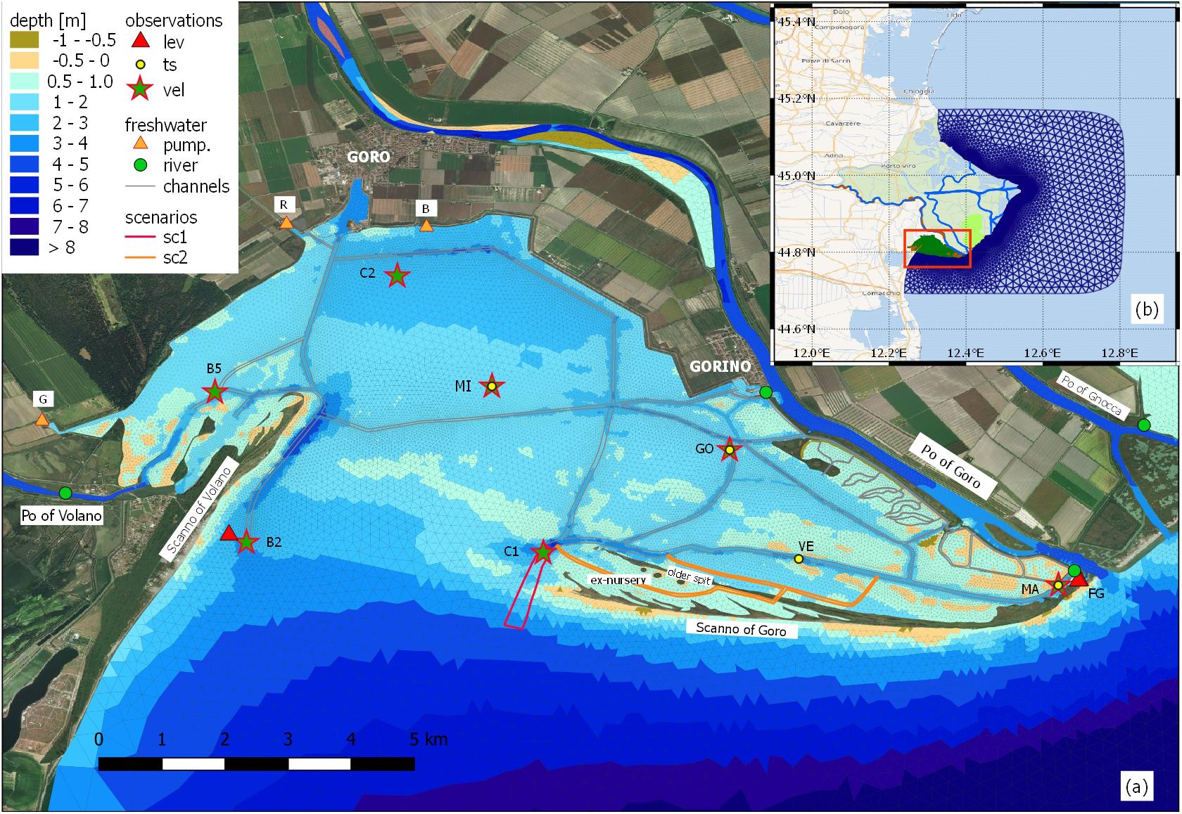
Figure 1. (A) Bathymetry of the triangular grid of the Goro Lagoon. In the upper panel (B), the grid extension of the model surrounding the Po river delta in the Northern Adriatic Sea. The pumping stations are: Giralda (G), Romanina (R), and Bonello (B). Station’s names are: Manufatto (MA), also a river connection (green point), Faro di Goro (FG), Venus (VE), Gorino (GO), nearby the Gorino lock (green point), Mitili (MI), Spiaggina di Goro (C2), western inlet channel (B2), and eastern inlet channel (C1). The Scanno of Goro is the most recent seaward spit that started to grow after 1991. The older spit is still present, but internal to the lagoon. The stars represent the points where the current meters were installed alone, CTD are indicated with the yellow dots. The background cartography comes from the Bing Aerial dataset for (A) and Wikimedia dataset for (B).
Exchange with the sea occurs through a 3 km wide and very shallow inlet, which is the submerged part of a previous spit that started to erode in 1991 after a channel had been dredged in the middle. At the same time a new seaward spit (the present Scanno of Goro) started to grow along the eastern coastline. The older spit is actually internal on the lagoon, and together with the Scanno of Goro occlude a valuable area devoted in the past to clam nurseries. This evolution is shown in the multiannual Landsat imagery slideshow retrievable with Google Earth. The overall accretion tendency of the Scanno of Goro is reported on the EMODnet Geology website1 and in Simeoni et al. (2007) and Bezzi et al. (2019).
Two channels are dredged on the inlet (Figure 1a). The bathymetry map shows the lower depth on the sea side of both channels, in particular the eastern one, meaning that there is a tendency toward occlusion because of the deposition of the sediments transported by coastal currents.
Similarly to the Po delta lagoons, the Goro lagoon has a small morphological variability (Maicu et al., 2018), the channel network is simple and the salt march area is not significant. Therefore, most of the lagoon volume (87%) is determined by the tidal flats, with an average depth of 1.5 m. The salt marches and intertidal flats occupy only 6% of the total area of the lagoon, which is going to furtherly diminish due to the combined effect of the subsidence (−8 mm/year, Tosi et al., 2016) and the sea level rise (≈ +6 mm/year, IPCC-AR5 estimation for the RCP 4.5, IPCC, 2013).
The Goro Lagoon has a large freshwater input, mainly from the Po of Volano in the western area and Po of Goro along the eastern boundary. Another four pumping stations are located on the mainland boundary (Figure 1a). The main connections with the Po of Goro river are the Gorino lock and the gate at the Goro lighthouse called “Manufatto,” which are managed manually by the local authorities to ensure the most favorable conditions for the lagoon productivity but unfortunately without recording. These gates are opened during the summer to enhance the water renewal, and are closed during the river floods to ensure an acceptable salinity in the lagoon and prevent sediment deposition.
The Goro Lagoon is continually evolving due to the multiple and variable forcings as well as human interventions aimed at enhancing the lagoon’s productivity. The physical interventions on the Goro Lagoon were first evaluated by O’Kane et al. (1992) with a 3D finite difference baroclinic model implemented on a 150 m-resolution grid. After a severe dystrophic crisis in 1992, the biological issues of the lagoon were initially studied with a zero-dimensional biogeochemical model by Zaldívar et al. (2003). Marinov et al. (2006) carried out another hydrodynamic characterization of the lagoon with a structured grid three dimensional model at 150 m resolution, coupled with a fate model to investigate the spatial distribution of several pesticides coming from the mainland (Carafa et al., 2006). Finally the model was coupled with a biogeochemical module in the work by Marinov et al. (2008). The above studies were the first comprehensive, step-by-step approach to implement a modeling chain capable of answering the main issues of the lagoon when the studies were made. However, the interconnection with the Adriatic Sea was approximated because no operational large-scale model of the Adriatic Sea was yet available for initial and lateral boundary conditions, making the results only a step toward the final solution.
The Downscaling Approach
The physical processes in the open ocean are driven by the so-called energy cascade (Vallis, 2006; Aluie et al., 2018) and occurs at several time and spatial scales depending on the location, the magnitude of the forcings and the stratification of the water column. In the marginal seas the bathymetric constrain and the freshwater inputs become relevant and can modify the circulation both at regional scale (Verri et al., 2018) and at larger scale (Huang and Mehta, 2010; Coles et al., 2013). An adequate representation of these processes should rely on numerical model capable to span between different spatial scales, such the ones shown in Bellafiore et al. (2021); Ferrarin et al. (2019), Maicu et al. (2018); Federico et al. (2017), Trotta et al. (2017), and Fortunato et al. (2017).
Goro Lagoon Finite Element Model was designed in order to fill the modeling gap between the previous “single compartment” approach of the Adriatic Sea sub-regional basin model, AdriaROMS (Chiggiato and Paolo, 2008; Russo et al., 2013) and the need for detailed geometry in the coastal areas of the Emilia Romagna coasts. The added value of GOLFEM lies in the smooth transfer of the offshore dynamics and thermohaline structure of the water column, down to the coast and finally into the lagoon and the river, at increasing model resolution for the detection of cross-scale processes (Valentini et al., 2007). This work is the result of a double downscaling, from the regional Copernicus CMEMS Mediterranean ocean model Med-MFC (Clementi et al., 2017) to the sub-regional model AdriaROMS and finally to GOLFEM.
AdriaROMS, is the Adriatic Sea model, which has been operational at the Hydro Meteo Climate Service of Arpae (Arpae-SIMC) since 2005. The model has a curvilinear horizontal grid with a resolution ranging from 2-km in the north Adriatic to 10 km in the south Adriatic and a vertical structure of 20 terrain-following levels. It is forced by COSMO-5M (COSMO Newsletter, 2004) at the surface, whereas at the open boundary at the Strait of Otranto, the temperature, salinity and velocity conditions are provided by the Mediterranean model MED-MFC. The main tidal components are derived from the Oregon State University (OSU) TPXO model (Egbert and Erofeeva, 2002) and added at the open boundary in Otranto. The Po River discharge is introduced as a source of mass and momentum using real time measurements and kept constant during each forecast. On the other hand, the runoff of another 48 rivers and karstic springs (along the eastern Adriatic coast) is introduced using monthly climatologies derived from the literature.
We designed a flexible modeling workflow that can be easily updated (bathymetry, coastline, and forcings) so that, on the one hand, it can produce reliable simulations for “what if” scenarios, and on the other hand, it is also capable to forecast extreme events (Valentini et al., 2007; Harley et al., 2016), flooding or dystrophic crises (Viaroli et al., 2001, 2006)
In this model workflow, the processes are added smoothly: for example in AdriaROMS four tidal components (S2, M2, O1, and K1) are added to the daily MED-MFC sea level at the Otranto Strait, the resolution of the meteorological forcing increases from 9 km (ECMWF for Med-MFC) to 5 km to force AdriaROMS. In GOLFEM, the tidal components are eight (see section “Lateral and Surface Forcing”), the river-sea interaction is modeled explicitly, and the atmospheric forcing is taken from a meteorological model at the horizontal resolution of 2.8 km (COSMO-I2, Steppeler et al., 2003).
Aims of the Paper
The first question addressed by this paper is the establishment of a solid understanding of the Goro lagoon dynamics, especially the interconnection of the lagoon circulation with the open sea. This was not possible until now, the previous models did not resolve such exchange, as mentioned before. Furthermore, we tried to understand how each forcing (tides, wind and freshwater inputs) acts on the seasonal lagoon dynamics and salinity distribution.
A second question is related to “what if” scenarios to evaluate the impacts of lagoon bathymetry changes. Assessing such scenarios assumes that the memory of the system is short enough so that the numerical simulations are done with different bathymetries or forcings with minor adjustment periods (memory of the initial conditions). The hydrodynamic changes are then statistically assessed within the assumption of a steady-state regime.
Observational Data and Numerical Model Setup
Observations
The calibration of GOLFEM is based on the data collected by the Regional Agency for Prevention, Environment and Energy of Emilia-Romagna (hereafter Arpae).
Bathymetry
The bathymetric representation is fundamental for a correct simulation of the circulation in this shallow lagoon where the bottom boundary layer affects the shallow water column.
We used several datasets and unified them into a single altimetric reference (Genova IGM, 1942) using appropriate offsets. In the open sea area, the EMODnet dataset at a 250 m resolution was merged with the coastal multibeam survey operated by Arpae in 2012, while in the lagoon, several single beam surveys were conducted by Arpae from 2004 to 2017. We merged these into a single sparse point dataset, considering most recent measurements when the data points overlap.
Along the river branches, we used the depth of the triangular elements of the numerical grid of Maicu et al. (2018). In the last 6 km of the Po of Goro branch, some single beam surveys were available, thus providing a reliable cross-section representation of the river.
Finally, we merged the three aforementioned collections and obtained a sparse point dataset that was interpolated on each triangular element of the mesh (Figure 1a).
Fixed and Temporary Stations
A field campaign was conducted in six stations during 2018 specifically for this project (Figure 1a). One current meter recorded a long time series at the Manufatto station, and the others recorded shorter time series. The instruments were deployed at fixed distance of one meter from the lagoon bottom. In addition, Arpae manages a network of fixed stations where the temperature and salinity are continuously recorded (yellow dots in Figure 1).
The sea level is measured by Arpae at the Goro lighthouse (FG in Figure 1), Porto Garibaldi (in the southwestern corner of the domain), and in Ariano Polesine, 40 km upstream of the Po of Goro branch. The tides in the northern Adriatic Sea have among the largest amplitudes in the Mediterranean Sea. The spectral analysis of the measured sea level in Porto Garibaldi shows that the largest tidal components are the lunar semi-diurnal M2 and the solar diurnal K1, and the maximum tidal range is about 1 m.
Freshwater Fluxes
The total discharge of the Po river (Figure 2) is computed using a discharge rate relation (Arpae, 2018) with the measured water level at Pontelagoscuro, 90 km upstream of the main river mouth. In 2018 the average discharge was 1533 m3s–1, very close to the mean of the reference period 1980–2010 (1,477 m3s–1). The discharge shows the typical moderate flood period from March to June due to the rainfall and snowmelt, and a significant discharge event in November. The river water temperature in Pontelagoscuro was measured by Arpae approximately every 15 days, from 1989 to 2011, and we thus calculated monthly climatological values which were imposed as lateral boundary condition. At the river upstream section the salinity was imposed to be zero.
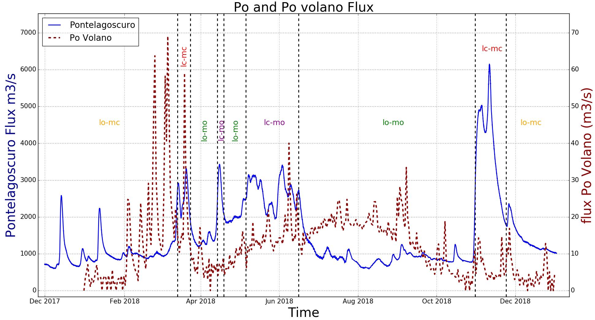
Figure 2. The blue line is the observed discharge of the Po River at Pontelagoscuro, 40 km upstream the Po di Goro branch. The red dotted line is the discharge of the Po di Volano, calculated as sum of the daily volumes of water pumped into the river. The vertical dashed lines represent the different configurations of the lagoon gates: lc-mc Gorino lock and Manufatto closed and vice versa lo-mo both open; lo-mc Gorino lock open and Manufatto closed and lc-mo vice versa.
The Po of Volano is the largest freshwater input into the Goro lagoon. It is an ancient river branch that now collects freshwater from several mainland pumping stations. The raw data (the functioning time of the pumping stations) were collected and the daily discharge was computed. The Po of Volano timeseries (Figure 2) shows several discharge peaks that take place prior to the Po river flood period and during the summer when the crops are irrigated: the mean flow in 2018 was about 12 m3s–1.
The 2018 average discharges were: Giralda 1.6 m3s–1, Romanina, 5.9 m3s–1, Bonello 0.5 m3s–1, Pomposa 0.24 m3s–1. The water temperature for the Po of Volano and Romanina plant was taken from the Arpae report on the water quality, where monthly data were reported since 2006. A monthly mean temperature was then computed and used as input for the model. The same temperature as the Romanina channel was also used for Giralda, Bonello and Pomposa pumping stations.
Riverine water enters the lagoon from the Po of Goro at the Gorino lock and Manufatto. The Gorino lock is closed during the high floods of the Po river and the Manufatto is partially closed approximately from November to March (personal communication). Without any other data available, we defined a threshold water level of +2.0 m m.s.l. measured in Ariano Polesine on the Po of Goro branch in order to detect the river floods and the closure periods of the Gorino lock and Manufatto.
The Numerical Model of the Goro Lagoon (GOLFEM)
The numerical model implemented here is based on the Shyfem code (System of Hydrodynamic Finite Element Modules2; Umgiesser et al., 2004; Cucco and Umgiesser, 2006), an unstructured grid model with triangular elements, capable of describing complex areas since it is possible to change easily the resolution of the elements (see Appendix A for model equations and parametrizations). The grid resolution spans from 2.2 km at the open boundary to less than 10 m in the narrowest channels inside the lagoon, with a total number of 77,496 elements.
The wide extension of the domain (Figure 1b) is needed to cover the entire delta Po area, which is the most important freshwater source discharging in the Adriatic Sea with a strong impact on the mass and salt balance of the area (Ludwig et al., 2009). The domain is also defined within the branches of the Po river.
The water column is represented vertically by 17 layers with a thickness ranging from 1 m in the upper 10 m, increasing to a maximum thickness of 7 m in the last layer. The first layer thickness changes with time according to the variations of the sea level due to tides, steric effects and atmospheric forcing. The absorption of the shortwave radiation follows a double exponential form (Paulson and Simpson, 1977) with attenuation coefficients ξ1 and ξ2 and a parameter R representing the percentage of entering radiation computed according to water type 9 in Jerlov (1976) (see Appendix A). The bottom stress is parametrized with a quadratic formulation and it is again described in details in Appendix A.
Due to the human operations of closing and opening the connections with the Po of Goro at Gorino lock and Manufatto, described in the previous section, different grids settings were established. Four different grid configurations were arranged: lo-mo, where Manuffato and the Gorino lock are both open; lo-mc, with the lock open and Manufatto closed; lc-mo, with the lock closed and the Manufatto open; lc-mc, with both the connections closed. These different grid settings were used based on the periods indicated in Figure 2, and for the water level threshold outlined in section “Freshwater Fluxes.”
Lateral and Surface Forcing
The initialization and the open boundary conditions are provided by AdriaROMS model analyses, with a 2.2 km of resolution, which in turn is nested at the Otranto strait CMEMS MED-MFS. GOLFEM is provided with the temperature, salinity and sea level as a Dirichlet boundary condition when the flow is directed toward the domain, while it is a zero-gradient condition at the boundary when the current flows out of the domain. The zonal and meridional velocities are nudged with a nudging time of 30 min.
In order to obtain the best tidal signal, a “detiding” procedure was applied to the AdriaROMS sea level using the Doodson filter (Doodson, 1928). The sea water level was then computed at the open boundary nodes adding the tidal signal (eight components: M2, S2, K2, N2, K1, O1, P1, and Q1) from the TPXO model (Egbert and Erofeeva, 2002), obtaining a more realistic sea level.
The river discharge is treated as an open boundary condition where transport and temperature are given by measurements (section “Freshwater Fluxes”) and the salinity is assumed to be zero. Since Po discharge is measured before the branching of the Po in the delta, a repartition relation was calculated to obtain the discharge of the Po of Goro as a function of the total discharge. This function was found with a cubic polynomial interpolation of the discharge measurements in the Po of Goro branch (ARPA Veneto, 2012), taken over several years but then interrupted.
The fluxes at the air-sea interface are treated with the MED-MFS bulk formulae (Pettenuzzo et al., 2010). The surface atmospheric fields are provided by COSMO-I2 meteorological model analysis at 2.8 km of horizontal resolution. The input variables are zonal and meridional velocity at 10 m, temperature and dewpoint temperature at 2 m, sea level atmospheric pressure, precipitation and total cloud cover.
Model Calibration
In a complex environment like the one described here, a comprehensive calibration of the model is needed. The first series of sensitivity experiments focused on the bottom friction roughness length λB (Appendix A). A period of 3 months was chosen for the calibration of the model, from 1 February 2018 to 1 May 2018. Values of λB ranging from 0.005 to 0.08 m were assigned to different areas of the domain, based on common sediment and known roughness characteristics. For each of the eight experiments, the model output was compared with the tide gauge and current observations in order to evaluate the model improvements. We found best values for λB in different areas: tidal flats 0.005 m, channels and open sea 0.01 m, rivers bed 0.02 m, river floodplains 0.08 m, saltmarshes 0.05 m, Manufatto and Gorino lock 0.015 m.
Other four sensitivity experiments were carried out for the tracer diffusion coefficient Kh with tested values of 0.2, 0.02, 0, and 1 m2s–1. In this case we compared temperature and salinity output with CTD observations. The differences between the sensitivity tests were negligible and the final value was chosen to be 0.2 m2s–1.
Model Validation
After the calibration, the model set up was validated over a 1-year simulation from 1 January 2018 to 1 January 2019. The statistical scores for the validation are defined in Appendix B and they are correlation R, root mean square error (RMSE), bias (BIAS), and mean absolute error (MAE).
Figure 3 compares the velocity, temperature, salinity, and sea level of the model output with the observations at two stations over the four available. Figures 3C,D show the temperatures for the whole year at station Manufatto and Mitili. In the winter months of 2018, the water temperature at the two stations was on average between 5 and 10°C with the lowest values of 2°C, while in August the values continuously exceeded 30°C, with peaks up to 32°C. We did not calculate the correlation R because the comparison between timeseries with strong seasonal signal (such as temperature) would mask an eventual modeling error giving rise to unrealistic large correlation value. The RMSE, BIAS, and MAE are shown in Table 1: the four stations average of BIAS, RMSE and MAE is −0.8, 1.3, and 1°C, respectively. This discrepancy can be due to several factors: the knowledge of the upstream condition for the water temperature at the Po of Goro boundary, the water temperature at the pumping stations, the open sea boundary condition that fluxes heat in the lagoon. It is plausible that the temperature errors are a combination of the aforementioned factors, each one with its own weight.
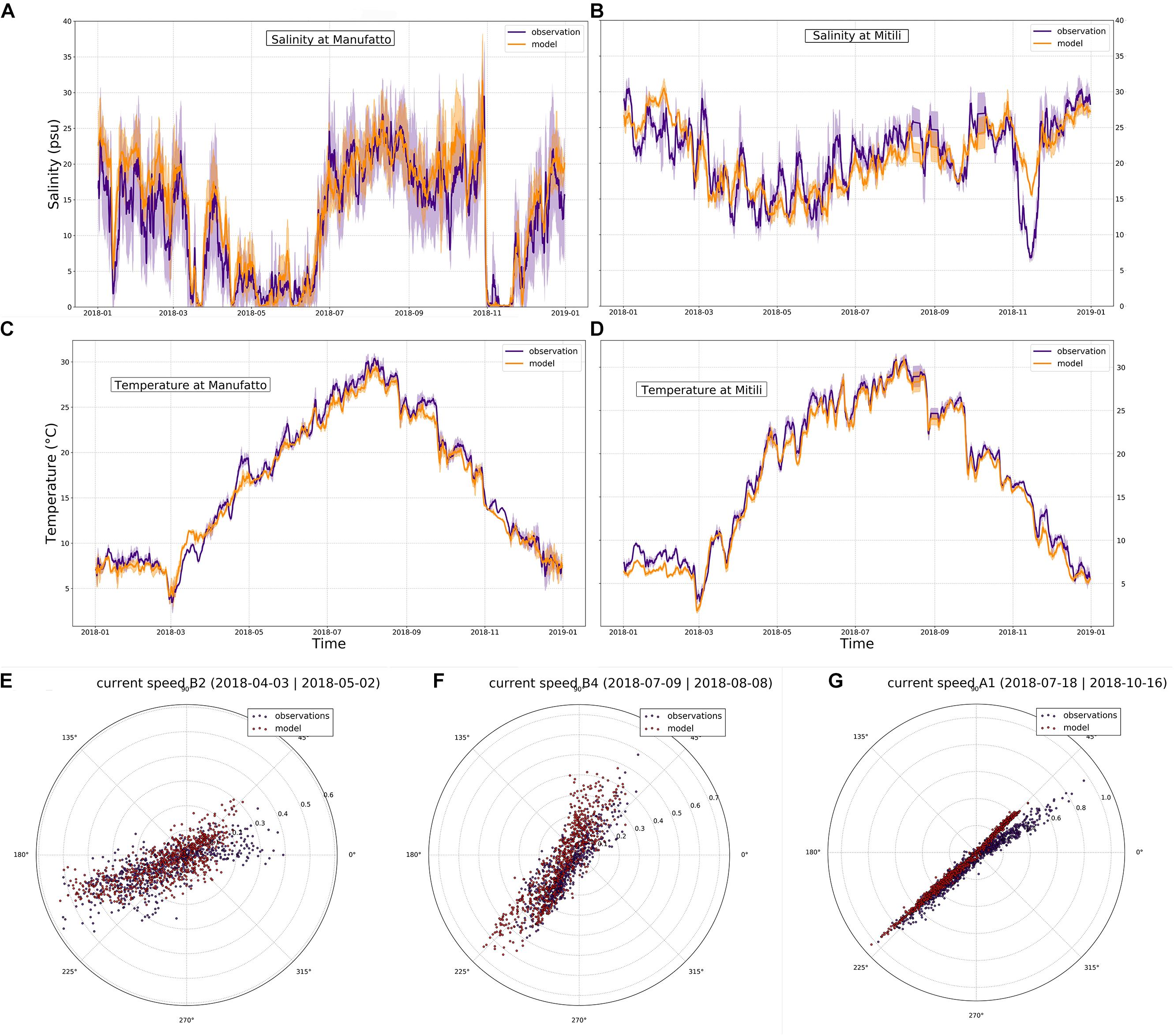
Figure 3. Comparison of observed and calculated salinity and temperature at the Manufatto (MA) (A,C) and Mitili (MI) (B,D) stations. The solid lines and the shaded areas are respectively the 24 h running mean and standard deviation. In panels (E–G), the comparisons of the polar plots of calculated and observed water velocity in the western inlet channel (B2), in the eastern inlet channel (B4) and Manufatto (MI or A1).
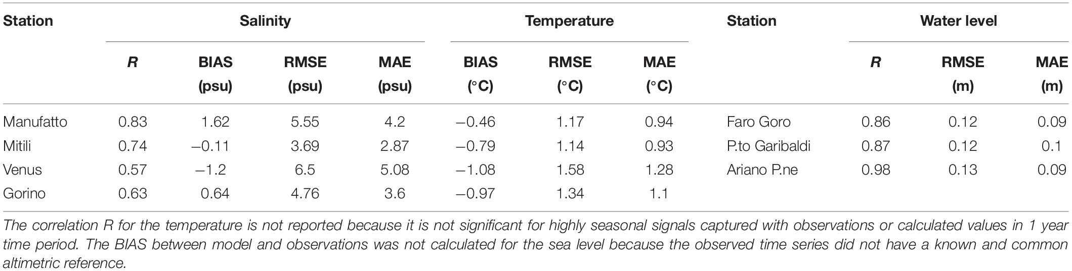
Table 1. Statistical scores for temperature and salinity and water level, as defined in Appendix B.
The salinity error is higher in absolute value than the one in temperature. The average R, BIAS, RMSE, and MAE shown in Table 1 amount to 0.7, 0.2, 5.1, and 3.9 PSU, respectively. These scores indicate that the model is saltier than observations and we argue that this is due to the unknown discharges and salinity values at the river mouths and the channels. However, Figures 3A,B show that the model is capable to follow the general structure of the salinity with sometimes big departures from the peak values, giving rise to large errors. This is quite evident in Figure 3B that shows a large mismatch between model results and observations occurring in November 2018 during a Po river flood. The Mitili station (MI in Figure 1a) is located in the central lagoon and several freshwater inputs concur to give maximum uncertainty especially for the Gorino Lock and the Manufatto gate where we do not have data on the opening/closing of the channels (see Figure 1).
Three tide gauges stations are considered for the validation of sea level: Porto Garibaldi, Ariano and Faro of Goro. The model shows a very good agreement with observations with a mean correlation of 0.9 and a RMSE of 0.12 m (Table 1). Further improvements in the sea level simulation could be obtained probably with an enhanced detiding procedure.
The velocity was compared with the current velocity and direction observations (Figure 1 for the position of the stations). Of the five observational points, only Manufatto, B2 (western inlet channel) and C1 (eastern inlet channel) were chosen for validation. The BIAS and RMSE are −0.11 and 0.28 ms–1, respectively for Manufatto, −0.01 and 0.12 ms–1 for B2 and 0.03 and 0.13 ms–1 for C1. Polar plots in Figures 3G–I show the comparison of the direction of the currents for stations B2, C1 and Manufatto, respectively. In general, there is a good agreement in the flow direction, which is mainly E-NE/W-SW for B2 and NE/SE for C1/B4.
Results
In this section, we study the circulation of the Goro lagoon and its thermohaline characteristics, highlighting the connections with the tidal, meteorological and hydrological forcing. These findings arise from the combination of two techniques. First the model downscaling propagates the sea level signal (including the large-scale meteorological surge) through the shelf into and the lagoon, and fully resolves the coastal mixing processes occurring outside the lagoon, in this multiple-mouths delta. Second the high-resolution modeling of the lagoon can resolve the hydrodynamics originated by several forcing in such complex environment with multiples connection to other water bodies.
The Goro Lagoon Circulation
Figure 4 highlights that the Goro lagoon is an estuarine basin with an average surface outflow and a bottom inflow. The baroclinic vertical structure of the velocity (Figure 4c) is at larger amplitude in the western inlet channel because of the deeper channel and the nearby freshwater inputs of the Po of Volano (see Figure 1a).
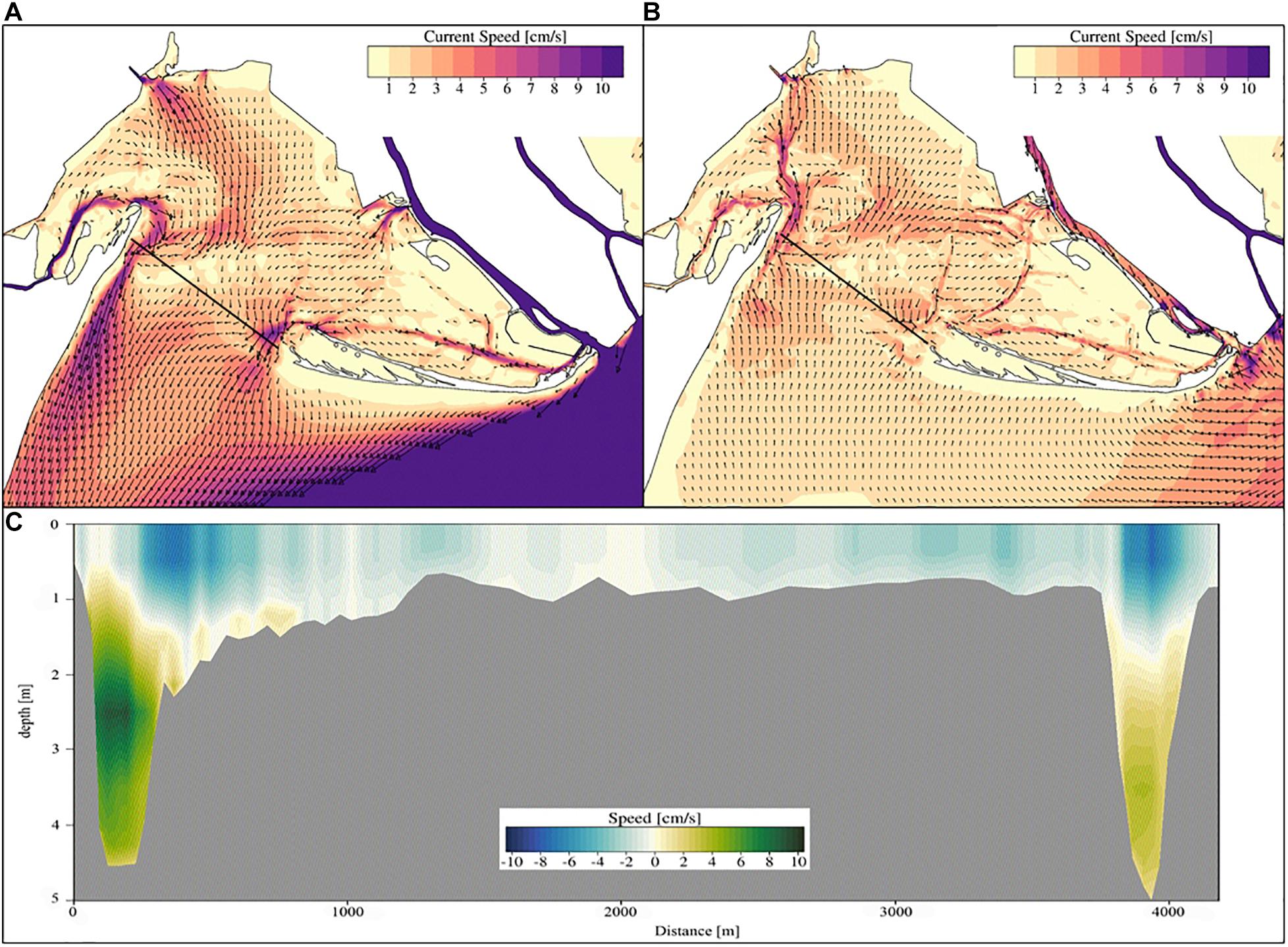
Figure 4. Average surface (A) and bottom (B) circulation, and (C) current speed along the inlet vertical cross section, indicated with the black line. Green colors indicate saltier water entering the lagoon, and blue colors indicate fresher water exiting the lagoon. Despite how it looks like in the panel (C), the western channel (“Bocca principale”) is deeper and wider with respect to the eastern channel (“Bocca secondaria”). Only few grid points of the western channel near the tip of the sand spit, are deeper than the western channel (Figure 1).
Harmonic analysis (Pawlowicz et al., 2002) of the simulated sea level in the harbors of Porto Garibaldi (outside the lagoon), Goro (northwest corner), and Gorino (northeast corner) show that the amplitudes of all the tidal components do not change between outside and inside the lagoon due to the flat bathymetry of the lagoon and the relative wide opening of the inlet (Table 2). Moreover, the tidal components have the same phase lag at Goro and Gorino meaning that the tidal signal is evenly transmitted throughout the lagoon. The circulation pattern is the same during spring and neap tide, with the current streamlines that spread from the main channel to the western and central area of the lagoon, and from the secondary channel toward Gorino and the eastern corner of the lagoon. The maximum current speed during the spring tide is about 0.8–1 ms–1 in the two inlet channels, while the speed does not exceed 0.2 ms–1 in most of the lagoon. Conversely, during neap tide, the circulation weakens but do not change, and the maximum current values decrease to 0.5 and 0.1 ms–1, respectively. No significant variation in the tidal circulation was detected at seasonal time scale.
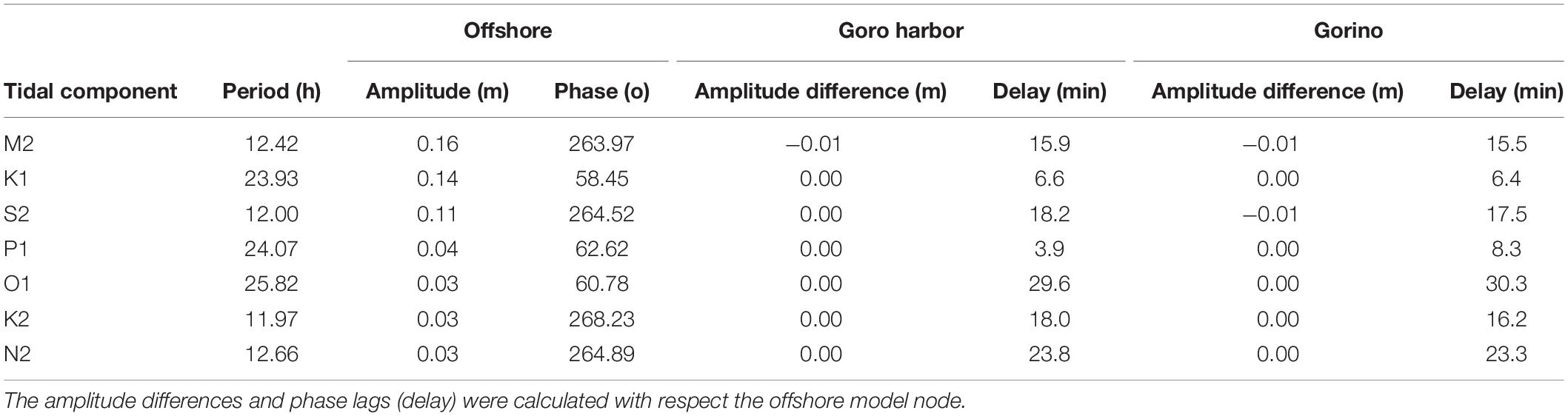
Table 2. Characteristics of the offshore tidal signal and its modification inside the lagoon.
Figure 5 shows that in the western inlet channel the flow is alternating between baroclinic and barotropic. During the neap tide period a baroclinic flow appears, manifested by the red and blue lines crossings in Figure 5. When the semidiurnal tidal signal is large, for most of the time the flow is barotropic either in or out of the lagoon, while when the signal is diurnal and the tidal range is reduced, the vertical structure of the flow can be baroclinic for major portions of the day, like it is shown in Figure 5 for February 7 or 9 of 2018.
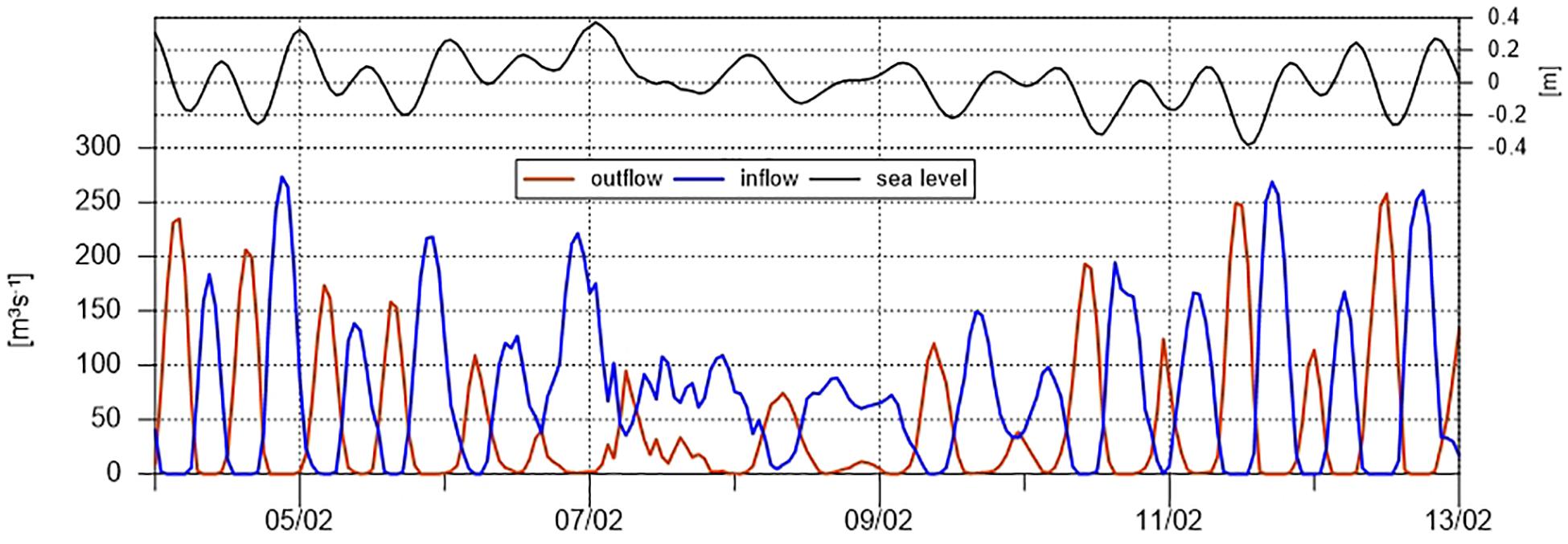
Figure 5. (Bottom panel) Time series of the net volume inflow/outflow in m3s– 1 calculated in the western inlet channel of the inlet section of Figure 4 and (top panel) sea level in m calculated at the sampling point B2, for 1 week (5–13) of February 2018.
Table 3 shows the magnitude and characteristics of the volume fluxes at the inlet section of Figure 4. The net flux of the western inlet channel is toward the lagoon (10.3 m3s–1) while in the remaining parts of the section the net flow is seaward. The central tidal flat is very shallow, so that no baroclinic circulation develops, and the flux is large toward the open sea (−39.2 m3s–1). In the eastern inlet channel, the net flux is also exiting the lagoon (−8.8 m3s–1).
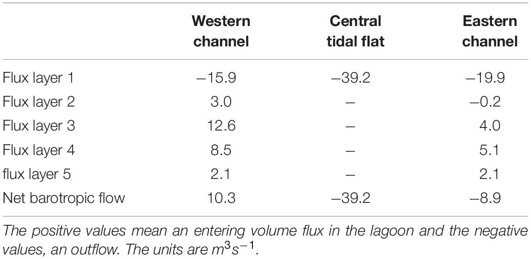
Table 3. Yearly mean volume fluxes through the three different portions of the section at the opening of the Goro Lagoon (Figure 1).
In conclusion the Goro lagoon is a large estuarine area with a net transport of water out of the lagoon equal to −37.8 m3s–1, the largest volume transport of open sea waters occurs in the western channel and the largest outflow of surface waters is from the central portion of the inlet section (Valle-Levinson, 2010; Valle-Levinson et al., 2015).
Being a land locked lagoon, the importance of winds in generating the circulation and the sea level change inside the lagoon cannot be underestimated. In the Adriatic Sea, the two dominant wind regimes, the Bora (NE), and Sirocco (SE) force the general circulation (Orlić et al., 1994; Ursella et al., 2006; Jeffries and Lee, 2007). The morphology of the Po Delta coastline significantly modifies the coastal current in front of the Goro Lagoon (Falcieri et al., 2013; Maicu et al., 2018; Bellafiore et al., 2019). The Bora strengthens the SW coastal current and piles up the water on the coastline south of the delta (Figure 6A). The effect of the Bora wind regime on the lagoon average circulation is to force the surface currents to exit the lagoon favoring in turn the advection of low salinity waters over the whole lagoon (Figure 6C). These meteorological conditions do not generally cause flooding in the Goro lagoon while the Sirocco does. Figure 6B shows that during an intense Sirocco, the lagoon is exposed to an average increase in sea level of up to 10 cm. During the peak of the event, the sea level difference between the Goro harbor and the shelf outside the lagoon reaches 20 cm. The wind driven average circulation at the inlet is mainly from the sea to the lagoon (Figure 6B) and higher salinity waters are advected into the lagoon (Figure 6D).
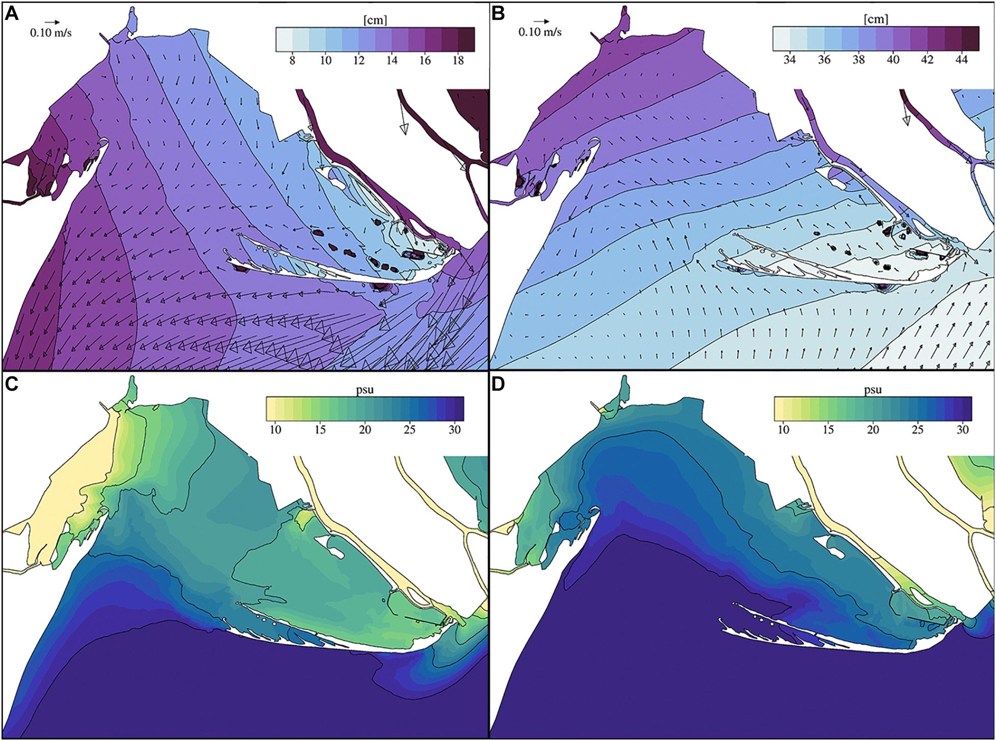
Figure 6. (A) mean sea level and (C) surface salinity field during an intense Bora wind event, occurred the February 22–26, 2018. (B) Means sea level and (D) surface salinity field during an intense Sirocco wind event, occurred the October 27–31, 2018.
The water renewal time (WRT; Cucco and Umgiesser, 2006) calculated with the high-resolution model and shown in Figure 7, confirms the findings of the previous work of Maicu et al., 2018, with a lagoon-averaged value of 5.8 days in 2018. The increase in the WRT occurs at the central part of the inlet section due to the bathymetric constraint of the tidal flat, while low WRT values in the marginal areas of the lagoon are ensured by the estuarine outflow generated by the riverine input of the Po of Volano and Po of Goro. The highest WRTs (10–12 days) are found in the ex-nursery area between the two sand spits of the Scanno of Goro and in a western basin between the Scanno of Volano and the Po of Volano river outflow (Figure 1).
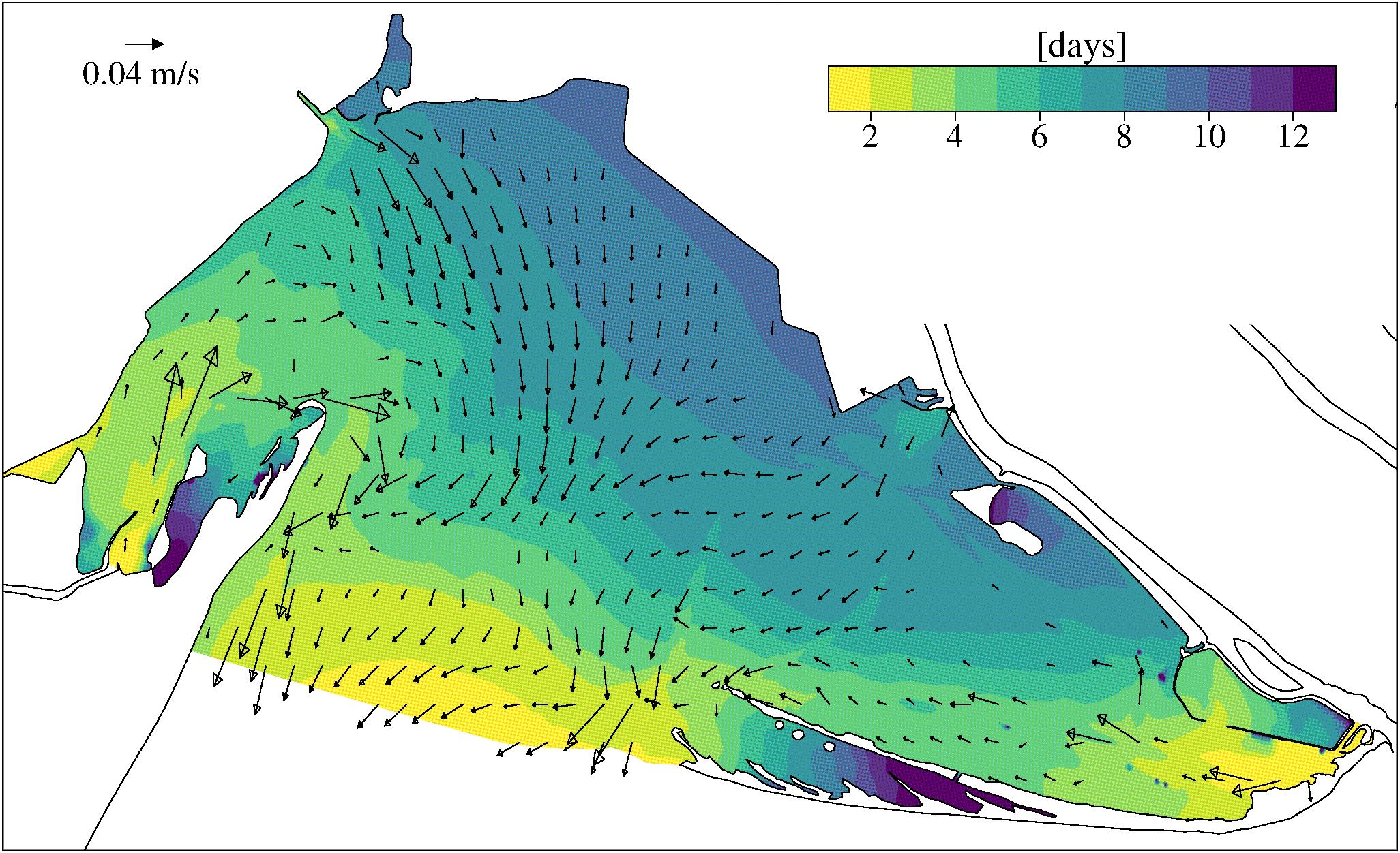
Figure 7. Average water renewal time and surface circulation calculated in 2018.
Salinity
The salinity pattern of the Goro lagoon is typical of an estuarine basin. Figure 8A shows that in most of the lagoon, the surface salinity is between 15 and 25 PSU. The only significant salinity gradient is in the western area where the salinity is less than 10 PSU and the salinity stratification (Figure 8B) occurs mainly in the deep channels. The diurnal standard deviation (i.e., the average over the simulated period of the standard deviation calculated on a daily basis) of the surface salinity (Figure 8C) highlights the areas where the mixing mainly occurs, i.e., in the central tidal flat and in particular along the western inlet channel. A large area of the lagoon has small daily salinity standard deviation (<1 PSU) meaning that there is almost no mixing. Outside the lagoon, the two areas with larger standard deviation indicate the occurrence of the mixing between the sea water and both lagoon and Po of Goro freshwater.
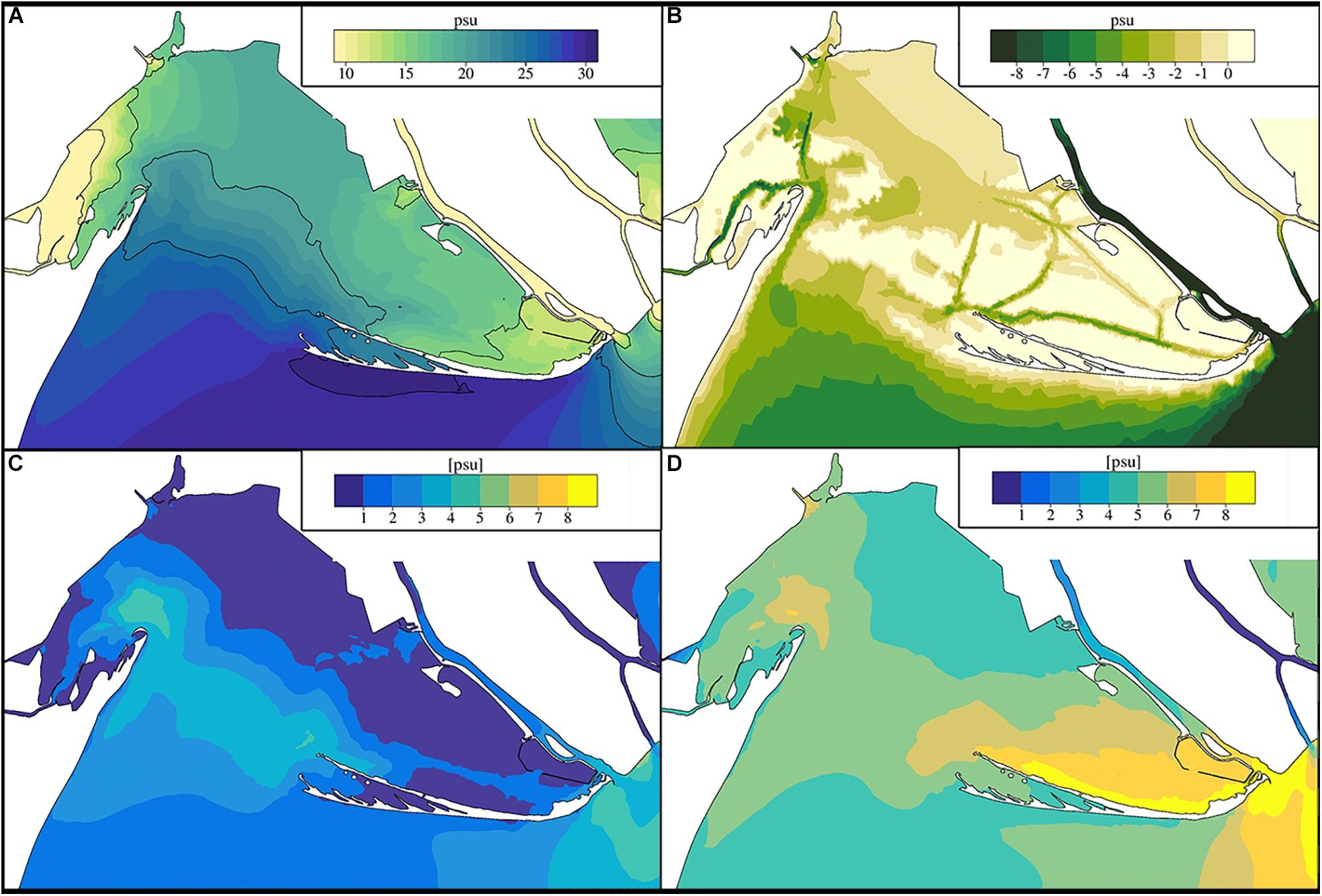
Figure 8. (A) Average surface salinity and (B) salinity vertical stratification shown as the difference between surface and bottom salinity. (C) Daily and (D) yearly standard deviation of the surface salinity, calculated averaging over the 2018 year.
On the other hand (Figure 8D), in the eastern basin of the lagoon, the yearly surface salinity standard deviation is significant (6–8 PSU), due to the seasonal variability of the freshwater inputs from the Po of Goro.
Figure 8C also shows the mixing in front of the Po of Goro mouth, where the tidal action and the southward along-shore current concur to mixing process of the freshwater river plume (Guarnieri et al., 2013; Bellafiore et al., 2019).
The high-resolution unstructured grid resolves the saltwater intrusion in the Po of Goro branch, even though the model was not calibrated for this purpose. Figure 9a shows that the seawater flows upstream at the river bottom, forcing the riverine water to accelerate downstream in the surface layer as the salinity increases due to the mixing. Between July and October 2018 the average discharge of the Po river was 845 m3s–1 (SD 130 m3s–1) and the average saltwater intrusion was about 13 km (Figure 9a). This fits very well with the distances measured by the provincial authorities of Ferrara between 2003 and 2009 in the corresponding range of the Po river discharge of 845 ± 130 m3s–1. The maximum extension of the salt wedge exceeded 20 km twice in August 2018 when the total Po river discharge was at a minimum of between 600 and 650 m3s–1.
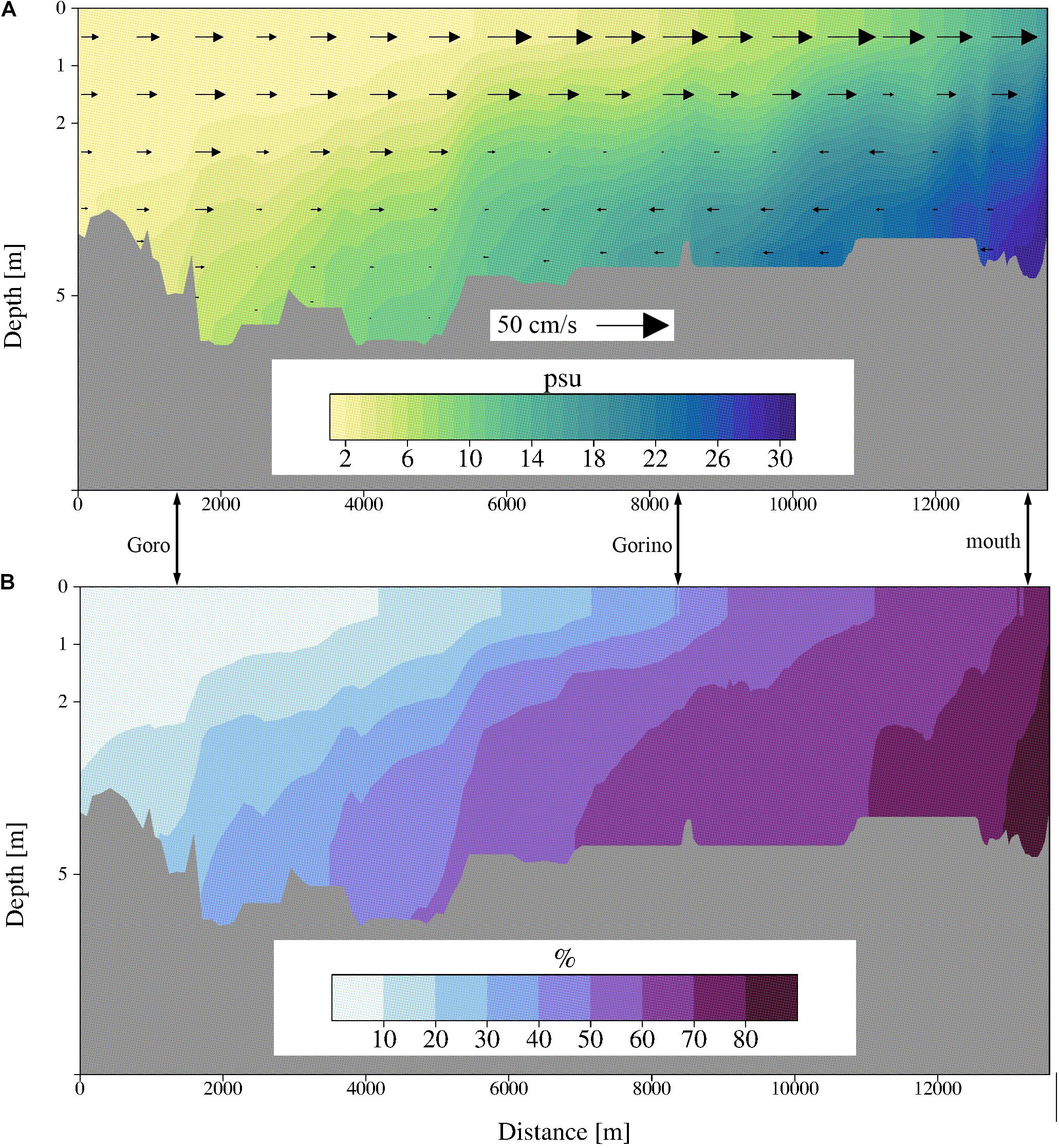
Figure 9. (A) Period July–October 2018: average salinity along the axis of the Po di Goro branch and superimposed average current. (B) Percentage of salinity values higher than 2 PSU along the axis of the Po di Goro branch during the 2018 year. Distances in m are from upstream to the river mouth.
In summary, the mean flow through the Gorino lock and the Manufatto gate transport waters that are brackish. The average salinity of the mean flow into the lagoon is 9 and 5.5 psu (mean flows 11.5 and 4 m3s–1) at the Manufatto and at the Gorino lock, respectively.
Temperature
The temperature stratification is smaller compared to the salinity vertical gradients, and is limited to the channels. The largest stratification (surface-bottom temperature) occurs when the lagoon vertical mixing is not yet effective in November and December (with a minimum vertical difference of −1.5°C, not shown) and also in April when the surface waters start to warm up (with maximum vertical gradients of about 1°C). The lowest and highest monthly temperature of the water column in the lagoon in 2018 occurred in February and August (Figures 10A,B) with basin averaged values of 6.0 and 27.9°C (basin standard deviation 0.68 and 0.24°C), respectively. Figure 10A also show that the difference of the water temperature between the lagoon and open sea is more relevant in winter (up to 4°C in December) while temperature in summer is similar.
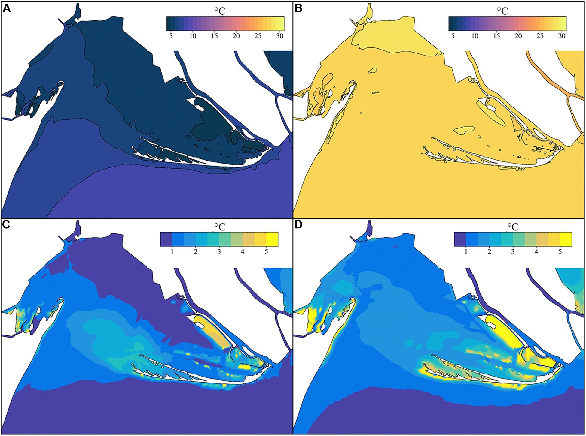
Figure 10. Average temperature of the water column in February (A), August (B) and average daily range (daily maximum – daily minimum) in February (C), August (D) 2018.
Figure 10C shows that during February the water column has a small (<2.5°C) daily range (difference between maximum and minimum temperature during 24 h) throughout most of the lagoon. In August (Figure 10D) the daily range of the temperature is slightly higher according to the larger daily range of the air temperature and the summer daily cycle heat fluxes. The daily variations of the water temperature in the lagoon depend both on the tidal inflow/outflow and the atmospheric heat fluxes in different areas of the lagoon and in different seasons. The largest daily range of the lagoon water temperature occurs in December (not shown) and is due to the combined effect of the tidal inflow (the open sea is warmer) and the daily cycle of the atmospheric forcing.
Understanding the Lagoon Circulation
The lagoon hydrodynamics is generated by the non-linear interaction of tides, freshwater inputs and winds. In this section, we aim to understand how each forcing influences the lagoon dynamics in the simulated period.
The average circulation is baroclinic in both inlet channels and in the lagoon during all months (Figure 11), meaning that the freshwater inputs are the main drivers of the estuarine circulation of Figure 4. The surface layer volume flux is highly variables and shows maximum peaks during the periods of larger freshwater inputs and vice versa, while the magnitude of the circulation at the bottom show less variability with respect to the 2018 average.
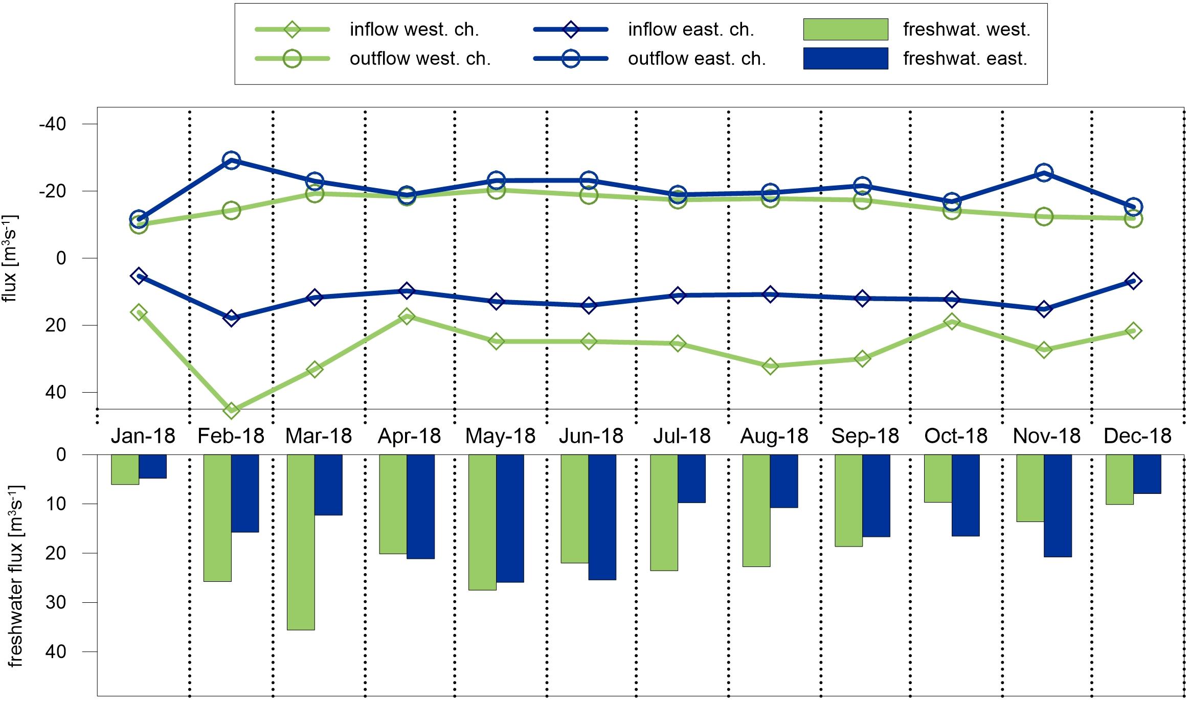
Figure 11. Average volume fluxes in the inlet channels, distinguished by inflow positive (in the deeper layers) and negative outflow in the surface layer. The average freshwater inputs in the lagoon are considered positive. The western freshwater is the sum of the Po of Volano and the pumping stations Giralda (G), Romanina (R), and Bonello (B) (Figure 1), The eastern freshwater is the sum of the volume fluxes at the Manufatto gate and Gorino lock.
Figure 11 shows that in the western inlet the surface lagoon outflow follows the seasonal freshwater cycle from Po of Volano and pumping stations, while in the eastern inlet the outflow is less correlated to the freshwater inputs from the Po of Goro discharge. This happens because the tidal and wind forcing induce a partial redistribution of the freshwater volume throughout the lagoon. The deeper inflow is largest in February, March, August and September, when the N-NE prevailing wind regime increases the lagoon-open sea density gradients, as shown in Figure 6C, that in turn enhances the baroclinic circulation. The supporting plots and data are available in the Supplementary Figures 1, 2.
We analyzed in detail the effects of the freshwater inputs on the circulation and salinity using GOLFEM in the period October 31–November 24, 2018 during a flood of the Po of Goro (Figure 2). In the best simulation case, the Gorino Lock and the Manufatto gates were closed during the Po flood (Figure 2) while in this experiment they both were left open, adding a freshwater inflow of +48 m3s–1 with respect to the previous configuration. The lower salinity in the central lagoon (from −6 to −10 PSU with respect to previous configuration) increases the horizontal density gradient with the open sea, and in turn the deep layer baroclinic inflow is larger.
The effect of the tidal forcing was then analyzed running two simulations with GOLFEM with and without tidal forcing, in the period May 6–June 6, 2018 where moderate freshwater inputs are found (Figure 2). In both simulations the Po of Goro connection were considered open. Without the tidal forcing the average freshwater inflow at the Manufatto gate increases (+8.4 m3s–1) decreasing the salinity. This is an indirect effect of tidal forcing on the salinity that is working in the same direction of an increased discharge. Outside the lagoon the salinity slightly increases (+1 PSU), so that the overall effect is the sharpening of the lagoon-sea density gradient, and strengthening in turn of the estuarine circulation. Interestingly the magnitude of the inflow increases in the second and third layers indicated in Table 3 because without tidal current the vertical mixing decreases and the water column stratification increases. This evidence is reported in the summary tables in the Supplementary Table 1.
Finally to study the effects of winds, we evaluated the WRT every 18 days, a time interval longer than the highest WRT, condition that is necessary for its correct estimation (Cucco and Umgiesser, 2006) and the correlation with the wind events. The timeseries of the basin-averaged WRT in 2018 confirm that the lowest values are in February and March when the N-NE wind drives the surface circulation out of the lagoon. Conversely, higher WRT values are found at the end of October with the Sirocco wind that opposes the surface outflow. Furthermore, the WRT anomalies (see Supplementary Figure 3) with respect to the average value of 2018 (Figure 7) demonstrate that the larger the freshwater inputs, the lower is the WRT at the basin scale because the average surface outflow is larger.
In conclusion, the characteristics of the estuarine circulation of the Goro Lagoon is determined by the simultaneous working of freshwater inputs, tidal forcing and winds. For the salinity, freshwater input is dominant but also tidal forcing that helps to decrease the inflow from the Po di Goro. For WRT, the wind forcing is crucial. Tidal forcing through its effect on the net runoff changes also the mixing in the Lagoon as recently explained for estuaries in Burchard (2020).
The Golfem Model for the “What If” Scenarios
The calibration and validation of the Goro Lagoon numerical model will facilitate “What if” scenarios to be carried out for the sustainable management of the site. The lagoon is a key area for clam farming in Italy. The economic activities are coordinated by a consortium of around 1400 local producers who, together with the local government authorities, helped to co-design the “What if” numerical experiments.
The ecosystem health and productivity levels of the lagoon are connected to the area’s morphology and dynamics, the hydrodynamic regime, the freshwater inputs, water salinity, and the specific ecosystem of the area. All these aspects interact to produce suitable conditions for the biological productivity of the lagoon. The question to be addressed by the “What if” scenarios is how to modify some of these key factors for the future sustainable exploitation of resources. To do this, a numerical model is needed that encompasses most of the interacting processes in the Lagoon, so that all the feedback can be considered. With a purely hydrodynamic model, like the one presented in this paper, we can address factors related to the morphology, the hydrodynamics, freshwater inputs, and the water salinity. In the future, if the complexity of the model is increased with sediment transport and ecosystem modeling, “What if” scenarios could be designed to answer additional management questions.
Local stakeholders wanted to know whether morphological interventions would have a positive impact on clam farming, and thus two morphology scenarios were investigated. The first scenario (Sc1) consisted in deepening and widening the eastern inlet channel (Figure 1a, red contour), which, as shown in the previous section, shows an important estuarine exchange with the open sea, with salt water entering at depth. Currently the eastern mouth has a width of about 50 m and a depth varying between a maximum of −5 m and a minimum of −1.5 m near the sea outlet, due to the littoral sand transport that is deposited in front of the inlet. The community of stakeholders asked what the hydrodynamics changes would be if the eastern mouth was enlarged to about 100 m, deepened up to 4 m everywhere and extended toward the sea (Figure 1a).
The second scenario (Sc2) consisted in dredging a channel that would extend from the eastern inlet channel to the easternmost side of the lagoon, crossing the area between the two spits of the Scanno of Goro, as shown by the orange line in Figure 1a. The stakeholders were interested to see whether the current and salinity conditions could be changed so that a clam nursery could be re-established between the spits. The stakeholders requested that the canal should have a width of 30 m and a depth of 3 m.
Numerical experiments were then carried out using these modifications in the model bottom bathymetry. The simulations were run for 2018 using the same atmospheric and river forcing as the present-day bathymetry conditions.
Differences between the present-day conditions and the scenarios were larger in Sc1 than Sc2 and in general were significant with respect to the mean current amplitudes in Figure 4 (current changes are of the order of 1–5 cm s–1). Differences were larger close to the specific bathymetry changes but some effects are evident, in the case of Sc1, in an area intercepted by a radius of about 2 km around the secondary mouth. Despite this, the increase in the tidal currents in the western channel is significant (8–10%) only in the peak values during the spring tide. The same analysis of the vertical structure of the flow carried out in Table 3 shows that there were no significant changes: the inflow increased slightly in the third level at the expense of the flow in the middle layers. The net flux of the eastern channel did not change appreciably (−9 m3 s–1).
These differences however, were not sufficiently insightful to understand whether the morphological changes would be worth the effort. It was then decided to use two “fitness (FT) indices” developed in a previous study (Istituto Delta Ecologia Applicata, 2004). The FTs considered here are threshold values for the current intensity and water salinity, which vary between 0 and 1 for sub-optimal to optimal clam farming conditions. We considered only FTs ranging from 0.5 to 1, for the barotropic current speed and the bottom salinity. The corresponding optimal values for current amplitudes (FT1) are between 20 and 150 cm s–1, and between 20 and 35 PSU for salinity (FT2). We then calculated the percentage of days in 2018 when FT1 and FT2 were above these optimal threshold values. The values of the FTs are shown in the Supplementary Figure 4.
Figure 12 shows the results for FT1 and FT2 in present day conditions and the difference between Sc1 and Sc2. The results confirm that today most of the farming areas are located where FT2 is higher than 60%. In contrast, FT1 seems to be a strong limiting factor for clam farming. This is partially true because normally the current speed is reduced to zero at each tidal inversion, and this lowers the percentage of days where the optimal FT1 values are achieved. In fact, the ex-nursery area is not favorable because of the very weak hydrodynamics, in agreement with the largest WRT values described before. Moreover, the areas of high riverine footprint are not suitable for clam farming, and the gates should be maneuvered carefully to ensure an acceptable value of FT2 during the early growing season of the clams.
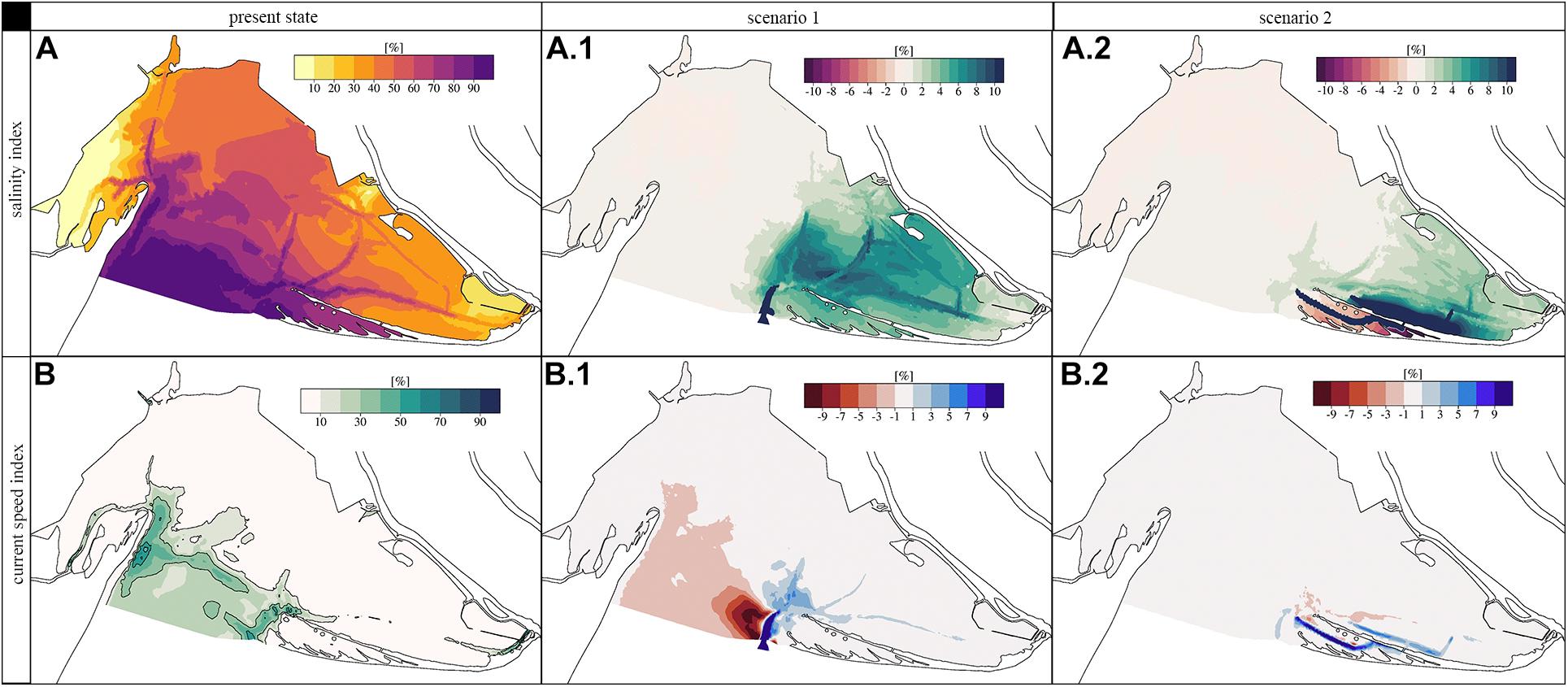
Figure 12. Fitness indices of optimal growing conditions of the present state for salinity (FT2) and current speed (FT1). (A) FT2 present day; (A.1) difference between FT2 in the present day and Sc1 conditions; (A.2) difference between FT2 in the present day and Sc2 conditions. (B) FT1 present day; (B.1) difference between FT1 in the present day and Sc1 conditions; (B.2) difference between FT1 in the present day and Sc2 conditions.
In Sc1, changes in FT1 and FT2 optimal conditions are of the order of 10–12% and in a quite extended area of the eastern lagoon. However, on the western side of the eastern mouth, there is a negative impact which needs to be considered. In Sc2, changes are more significant for FT2 (up to +15% changes) but only in an area close to the bathymetry changes and not as wide area as in Sc1. In Sc2 FT1 changes are negligible.
Using only FT1 and FT2 indices for the Goro Lagoon, the preliminary conclusion is that multiple interventions would be required, and that local dredging would simply not induce large enough changes to impact on the optimal functioning of the lagoon.
Summary and Conclusion
In this paper we studied the circulation of the Goro lagoon and its connectivity with the open sea and we carried out “what if” scenarios for the optimal functioning of the lagoon as a clam farming site.
The Goro lagoon was modeled for the first time with the appropriate connections to the open ocean waters. This has been realized by a cascading model strategy from the large-scale ocean circulation, at the Mediterranean scale (CMEMS analyses), to the Adriatic intermediate model (AdriaROMS) and to the Goro lagoon marine areas with unstructured grid modeling. This model cascading is necessary to add processes at different space and time scales where and when it is needed. GOLFEM has 10 m resolution inside the lagoon, required to resolve the channels, and high frequency winds, as well as resolved interfaces with both the riverine inputs and the open sea.
The Goro lagoon is found to be an estuarine dominated area where exchanges with the open sea occur along two relatively deep lateral channels (5–6 m deep) and one shallow central tidal flat plateau. Across the latter there is only outflow of lagoon waters while at the two side channels along the inlet section, the flow is on average baroclinic. Open sea, relatively salty waters are exchanged from the bottom of the channels to about 2–3 m from the surface and this is the only source of open sea water entering the lagoon on a yearly average.
The tidal flow in the lagoon is dominated by semidiurnal tidal components and it is an important high frequency component of the circulation. The exchanges at the inlet section channels can be barotropic and baroclinic at different phases of the tidal flow and there are also hours of the day where the net flow through the inlet section is minimum and some days it remains baroclinic for several hours. The lagoon WRTs are from few days to more than a week, signaling the importance of the deep water inflow from the channels for the exchange of oxygen with the open sea waters.
The lagoon-river channels exchanges were analyzed and the mean values of the discharges and their salinities were calculated: the average river-channel volume flux enters the lagoon trough the Gorino lock and the Manufatto and the water is brackish because of the seawater intrusions in the Po of Goro branch. The salinity intrusion exceeded 20 km in August 2018 with the lowest discharge from the Po. Considering that the climate change scenarios project decreasing Po river discharges due to atmospheric drought conditions, the amplitude of the salt wedge is clearly a severe threat to the lagoon.
The results of this work are reliable and derive not only from the high resolution of the model, but also from the detailed knowledge of the lateral boundary conditions. Nevertheless, there is still uncertainties. Since the fast-evolving morphology is an important constraint on the lagoon dynamics, continuously updated, synoptic bathymetric surveys are fundamental, rather than multiple patch-like surveys. In addition to the natural variability of the hydrological forcing, the untracked opening/closing of the Gorino lock and Manufatto operated by the local authorities, are another source of uncertainty in simulating the circulation of the lagoon.
The changes in the circulation due to man-induced changes in bathymetry happen very rapidly due to the shallowness of the Lagoon and its fast WRTs. The assessment of the long period effects of bathymetric changes on the circulation implies morphological modeling and sediment transport, with all the assumptions regarding the sediment load boundary conditions from the river branches. This will be part of future investigations that are prepared by the present work in terms of a solid hydrodynamic modeling, coherent with the present data.
Goro Lagoon Finite Element Model was also conceived as a scientific tool to support decision makers in evaluating interventions for improving clam farming and the sustainable exploitation of the Goro lagoon. The high-resolution triangular grid can be easily adapted to represent the features of new channels that need dredging or deepening.
The “What if” scenarios described in this paper show that realistic and complex validated/calibrated hydrodynamic numerical models can help to reduce uncertainties regarding the impacts of different interventions. The difference with previous studies is that now the uncertainty related to the reproduction of the present day environmental marine conditions has been lowered to an acceptable value. The “What if” scenarios examined in this paper highlight that dredging might not always imply a change in hydrodynamic conditions leading to a significant change in fitness indices. The local dredging of canals inside the Scanno of Goro is clearly not sufficient to increase the current intensity and the salinity values to more suitable conditions for the clam farming of the lagoon.
Finally, this study demonstrates the importance of designing a seamless chain of models that integrate local effects into the initial fields derived from coarser operational models. Furthermore it poses already questions on the essential monitoring aspects of the lagoon which should consider bathymetric frequent surveys and a strict management of the man-made channel inflows. We believe that our findings demonstrate that the proper cascading approach can be a valid modeling methodology to face the challenges of predicting the Global Coastal Ocean in the next decade.
Data Availability Statement
A public repository named “Downscaling of an unstructured model from the coastal-ocean to the Goro lagoon and the Po river delta branches (Italy): results of the GOLFEM finite element model” was created and is accessible at doi: 10.5281/zenodo.4072016.
The dataset comprehends the model outputs and the postprocessed results, converted in regular grid format (Netcdf) at 100 m and 50 m resolution, respectively, the time series of the freshwater discharges calculated on the basis of the raw data of the pumping stations, and the climatological time series of the water temperature for the Po river and the pumping stations.
Author Contributions
NP, FM, and GU the study was designed (conceptualization and methodology). ST and SL were responsible for the field campaign and the collection of the data, that were analyzed by JA and FM. JA and FM performed the model setup, validation, and simulations. FM, NP, and JA conducted the analysis and discussion of the model results. FM wrote the Abstract, sections “Introduction,” “Observations,” “Results,” and “The Golfem Model for the ‘What If’ Scenarios”. JA wrote the section “The Numerical Model of the Goro Lagoon (GOLFEM),” and “Appendixes”, reviewed by GV. NP wrote the section “Understanding the Lagoon Circulation.” AV wrote the section “The Downscaling Approach.” AV and TP were responsible for the project and the study as well as, together with SL, for the fundraising and the collaboration among CNR, UNIBO, and Arpae, and with the local stakeholders of the Goro Lagoon. All authors contributed to the article and approved the submitted version.
Funding
The GOLFEM model was realized thanks to the funds granted by the Emilia-Romagna law “L.R. 36/1995 e s.m.i. – Piano Operativo 2016–2017 – Anno 2017” and transferred to Arpae as decided by the “Comitato Operativo Sacca di Goro” in September 2017. Arpae, in turn, involved the Department of Physics and Astronomy of the University of Bologna and the Institute of Marine Sciences (Venice) of the National Research Council for the development of the model.
Conflict of Interest
The authors declare that the research was conducted in the absence of any commercial or financial relationships that could be construed as a potential conflict of interest.
Acknowledgments
We would like to thank the local stakeholders that helped to focus the work on important socio-economic activities, the improvement of the ecological value and the correct exploitation of the Goro Lagoon. We cite the Major of Goro, the technical office of the Goro Munipality, the local fisherman’s consortium CO.Sa.Go., the Istituto Delta Ecologia Applicata for the valuable support, field information’s transfer and the results discussions. Furthermore, we would also like to thank Dr. Paola Magri of the Arpae (local office of Ferrara) for the helpful interaction with the local stakeholders, the personnel of the Struttura Oceanografica Daphne – Unità Sacca di Goro, for the field campaign and information. We would also like to thank Eng. Laura Montanari from Consorzio di Bonifica Pianura di Ferrara for supplying the useful information about the drainage basin of the Goro Lagoon and the important data of the pumping stations. The GOLFEM simulations were mostly run on the Galileo supercomputer at the SCAI facility of CINECA in Bologna, freely available for the Ph.D. students at the University of Bologna, and on the Arpae-SIMC supercomputing facility.
Supplementary Material
The Supplementary Material for this article can be found online at: https://www.frontiersin.org/articles/10.3389/fmars.2021.647781/full#supplementary-material
Footnotes
References
Aleynik, D., Dale, A. C., Porter, M., and Davidson, K. (2016). A high resolution hydrodynamic model system suitable for novel harmful algal bloom modelling in areas of complex coastline and topography. Harmful Algae 53, 102–117. doi: 10.1016/j.hal.2015.11.012
Alfieri, L., Salamon, P., Pappenberger, F., Wetterhall, F., and Thielen, J. (2012). Operational early warning systems for water-related hazards in Europe. Environ. Sci. Policy 21, 35–49. doi: 10.1016/j.envsci.2012.01.008
Aluie, H., Hecht, M., and Vallis, G. K. (2018). Mapping the energy cascade in the north atlantic ocean: the coarse-graining approach. J. Phys. Oceanogr. 48, 225–244. doi: 10.1175/JPO-D-17-0100.1
ARPA Veneto (2012). Agenzia Regionale per la Prevenzione e Protezione Ambientale del Veneto, Dipartimento Regionale per la Sicurezza del Territorio. Sulla Ripartizione Delle Portate del Po tra i vari Rami e le Bocche a Mare del Delta: Esperienze Storiche e Nuove Indagini All’anno 2011. Relazione 02/2012. Vicenza: ARPA Veneto.
Arpae (2018). Agenzia Regionale per la Prevenzione, l’Ambiente e l’Energia dell’Emilia Romagna, Struttura Idro-Meteo-Clima, Servizio Idrografia e Idrologia Regionale e Distretto Po. Annali Idrologici 2018, Parte Seconda. Bologna: Arpae.
Aubrey, D. G., and Friedrichs, C. T. (1996). Buoyancy Effects on Coastal and Estuarine Dynamics. Washington, DC: American Geophysical Union. doi: 10.1029/CE053
Bellafiore, D., Ferrarin, C., Braga, F., Zaggia, L., Maicu, F., Lorenzetti, G., et al. (2019). Coastal mixing in multiple-mouth deltas: a case study in the Po delta, Italy. Estuar. Coast. Shelf Sci. 226:106254. doi: 10.1016/j.ecss.2019.106254
Bellafiore, D., Ferrarin, C., Maicu, F., Manfè, G., Lorenzetti, G., Umgiesser, G., et al. (2021). Saltwater intrusion in a Mediterranean delta under a changing climate. J. Geophys. Rese. Oceans 126:e2020JC016437. doi: 10.1029/2020JC016437
Bezzi, A., Casagrande, G., Martinucci, D., Pillon, S., Del Grande, C., and Fontolan, G. (2019). Modern sedimentary facies in a progradational barrier-spit system: goro lagoon, Po delta, Italy. Estuar. Coast. Shelf Sci. 227:106323. doi: 10.1016/j.ecss.2019.106323
Blumberg, A. F., and Mellor, G. L. (1987). “A description of a three-dimensional coastal ocean circulation model,” in Coastal and Estuarine Sciences, Book 4, ed. N. S. Heaps (Washington, DC: American Geophysical Union), 1–6.
Burchard, H. (2020). A universal law of estuarine mixing. J. Phys. Oceanogr. 2, 81–93. doi: 10.1175/JPO-D-19-0014.1
Burchard, H., Bolding, K., and Villarreal, M. (1999). GOTM-A General Ocean Turbulence Model. Theory, Applications and Test Cases. European Commission Report EUR. Luxembourg: European Commission.
Carafa, R., Marinov, D., Dueri, S., Wollgast, J., Ligthart, J., Canuti, E., et al. (2006). A 3D hydrodynamic fate and transport model for herbicides in Sacca di Goro coastal lagoon (Northern Adriatic). Mar. Pollut. Bull. 52, 1231–1248. doi: 10.1016/j.marpolbul.2006.02.025
Chiggiato, J., and Paolo, O. (2008). Operational ocean models in the Adriatic Sea: a skill assessment. Ocean Sci. 4:2008. doi: 10.5194/os-4-61-2008
Clementi, E., Oddo, P., Drudi, M., Pinardi, N., Korres, G., and Grandi, A. (2017). Coupling hydrodynamic and wave models: first step and sensitivity experiments in the Mediterranean Sea. Ocean Dynamics 67, 1293–1312. doi: 10.1007/s10236-017-1087-7
Coles, V. J., Brooks, M. T., Hopkins, J., Stukel, M. R., Yager, P. L., and Hood, R. R. (2013). The pathways and properties of the Amazon River Plume in the tropical North Atlantic Ocean. J. Geophys. Res. Oceans 118, 6894–6913. doi: 10.1002/2013JC008981
Correggiari, A., Cattaneo, A., and Trincardi, F. (2005). The modern Po Delta system: lobe switching and asymmetric prodelta growth. Mar. Geol. 222–223, 49–74. doi: 10.1016/j.margeo.2005.06.039
COSMO Newsletter (2004). Operational applications – ARPA-SIM (BOLOGNA). Deutsch. WetterDienst (DWD) Offenbach 6, 25–26.
Cucco, A., and Umgiesser, G. (2006). Modeling the venice lagoon residence time. Ecol. Model. 193, 34–51. doi: 10.1016/j.ecolmodel.2005.07.043
Doodson, A. T. (1928). The Analysis of Tidal Observations: Series A, Containing Papers of a Mathematical or Physical Character227223–279. London: Philosophical Transactions of the Royal Society. doi: 10.1098/rsta.1928.0006
Egbert, G. D., and Erofeeva, S. Y. (2002). Efficient inverse modeling of barotropic ocean tides. J. Atmosph. Oceanic Technol. 19, 183–204. doi: 10.1175/1520-04262002019<0183:EIMOBO<2.0.CO;2
Falcieri, M. F., Benettazzo, A., Sclavo, M., Russo, A., and Carniel, S. (2013). Po river plume pattern variability investigated from model data. Contin. Shelf Res. 87, 84–95. doi: 10.1016/j.csr.2013.11.001
Federico, I., Pinardi, N., Coppini, G., Oddo, P., Lecci, R., and Mossa, M. (2017). Coastal ocean forecasting with an unstructured grid model in the southern Adriatic and northern Ionian seas. Nat. Hazards Earth Syst. Sci. 17, 45–59. doi: 10.5194/nhess-17-45-2017
Ferrarin, C., Davolio, S., Bellafiore, D., Ghezzo, M., Maicu, F., Mc Kiver, W., et al. (2019). Cross-scale operational oceanography in the Adriatic Sea. J. Operat. Oceanogr. 12, 86–103. doi: 10.1080/1755876X.2019.1576275
Fofonoff, N. P., and Millard, R. C. Jr. (1983). Algorithms for the Computation of Fundamental Properties of Seawater. UNESCO Technical Papers in Marine Sciences, Vol. 44. Available online at: http://hdl.handle.net/11329/109
Fortunato, A., Oliveira, A., Rogeiro, J., Tavares da Costa, R., Gomes, J. L., Li, K., et al. (2017). Operational forecast framework applied to extreme sea levels at regional and local scales. J. Operat. Oceanogr. 10, 1–15. doi: 10.1080/1755876X.2016.1255471
Guarnieri, A., Pinardi, N., Oddo, P., Bortoluzzi, G., and Ravaioli, M. (2013). Impact of tides in a baroclinic circulation model of the Adriatic Sea. J. Geophys. Res. Oceans 118, 166–183. doi: 10.1029/2012JC007921
Harley, M. D., Valentini, A., Armaroli, C., Perini, L., Calabrese, L., and Ciavola, P. (2016). Can an early-warning system help minimize the impacts of coastal storms? A case study of the 2012 Halloween storm, northern Italy. Nat. Hazards Earth Syst. Sci. 16, 209–222. doi: 10.5194/nhess-16-209-2016
Hellerman, S., and Rosenstein, M. (1983). Normal monthly wind stress over the world ocean with error estimates. J. Phys. Oceanogr. 13, 1093–1104. doi: 10.1175/1520-04851983013<1093:NMWSOT<2.0.CO;2
Huang, B., and Mehta, V. M. (2010). Influences of freshwater from major rivers on global ocean circulation and temperatures in the MIT ocean general circulation model. Adv. Atmos. Sci. 27, 455–468. doi: 10.1007/s00376-009-9022-6
IPCC (2013). Climate Change 2013: The Physical Science Basis. Contribution of Working Group I to the Fifth Assessment Report of the Intergovernmental Panel on Climate Change. Cambridge: Cambridge University Press.
Istituto Delta Ecologia Applicata (2004). Relazione Finale-Studio delle Potenzialità Produttive della Sacca di Goro. Ferrara: Istituto Delta Ecologia Applicata.
Jeffries, M. A., and Lee, C. M. (2007). A climatology of the northern Adriatic Sea’s response to bora and river forcing. J. Geophys. Res. Oceans. 112:C03S02. doi: 10.1029/2006JC003664
Kjerfve, B., and Magill, K. E. (1989). Geographic and hydrodynamic characteristics of shallow coastal lagoons. Mar. Geol. 88, 187–199. doi: 10.1016/0025-3227(89)90097-2
Kolmogorov, A. N. (1941). Equations of turbulent motion on an incompressible fluid, I Dokl. Akad. Nauk SSSR 30, 299–303, (English Translation: Imperial College, Mech. Eng. Dept. Rept. ON/6, 1968).
Ludwig, W., Dumont, E., Meybeck, M., and Heussner, S. (2009). River discharges of water and nutrients to the Mediterranean and Black Sea: major drivers for ecosystem changes during past and future decades? Progr. Oceanogr. 80, 199–217. doi: 10.1016/j.pocean.2009.02.001
Maicu, F., De Pascalis, F., and Ferrarin, C. (2018). Hydrodynamics of the po river-delta-sea system. J. Geophys. Res. Oceans. 123:3601. doi: 10.1029/2017JC013601
Marinov, D., Norro, A., and Zaldivar, J.-M. (2006). Application of COHERENS model for hydrodynamic investigation of Sacca di Goro coastal lagoon (Italian Adriatic Sea shore). Ecol. Model. 193, 52–68. doi: 10.1016/j.ecolmodel.2005.07.042
Marinov, D., Zaldivar, J. M., Norro, A., Giordani, G., and Viaroli, P. (2008). Integrated modelling in coastal lagoons: Sacca di Goro case study. Hydrobiologia 611, 147–165. doi: 10.1007/s10750-008-9451-8
O’Kane, J. P., Suppo, M., Todini, E., and Turner, J. (1992). Physical intervention in the lagoon of Sacca di Goro. An examination using a 3-D numerical model. Mar. Coast. Eutrophic. 126, 489–510. doi: 10.1016/B978-0-444-89990-3.50046-8
Orlić, M., Kuzmić, M., and Pasarić, Z. (1994). Response of the Adriatic Sea to the bora and sirocco forcing. Contin. Shelf Res. 14, 91–116. doi: 10.1016/0278-4343(94)90007-8
Paulson, C. A., and Simpson, J. J. (1977). Irradiance measurements in the upper ocean. J. Physical Oceanography 7, 952–956. doi: 10.1175/1520-04851977007<0952:IMITUO<2.0.CO;2
Pawlowicz, R., Beardsley, B., and Lentz, S. (2002). Classical tidal harmonic analysis including error estimates in MATLAB using T_TIDE. Comput. Geosci. 28, 929–937. doi: 10.1016/S0098-3004(02)00013-4
Pettenuzzo, D., Large, W. G., and Pinardi, N. (2010). On the corrections of ERA-40 surface flux products consistent with the Mediterranean heat and water budgets and the connection between basin surface total heat flux and NAO. J. Geophys. Res. Oceans 115:6022P. doi: 10.1029/2009JC005631
Prandtl, L., and Wieghardt, K. (1945). Über ein neues Formelsystem f⋅ur die ausgebildete Turbulenz. Nachr. Akad. Wiss. Göttingen Math. Phys. Kl. 1, 6–19. doi: 10.1007/978-3-662-11836-8_72
Reed, R. K. (1977). On estimating insolation over the Ocean. Phys. Oceanogr. 7, 482–485. doi: 10.1175/1520-0485(1977)007<0482:OEIOTO>2.0.CO;2
Russo, A., Coluccelli, A., Carniel, S., Benetazzo, A., Valentini, A., Paccagnella, T., et al. (2013). Operational Models Hierarchy for Short Term Marine Predictions: The Adriatic Sea Example. MTS/IEEE OCEANS – Bergen. Bergen: IEEE, 1–6. doi: 10.1109/OCEANS-Bergen.2013.6608139
Sánchez-Arcilla, A., García-León, M., Gracia, V., Devoy, R., Stanica, A., and Gault, J. (2016). Managing coastal environments under climate change: pathways to adaptation. Sci. Total Environ. 572, 1336–1352. doi: 10.1016/j.scitotenv.2016.01.124
Simeoni, U., Fontolan, G., Tessari, U., and Corbau, C. (2007). Domains of spit evolution in the Goro area, Po Delta, Italy. Geomorphology 86, 332–348. doi: 10.1016/j.geomorph.2006.09.006
Smagorinsky, J. (1963). General circulation experiments with the primitive equation i the basic experiment. Month. Weather Rev. 91, 99–164. doi: 10.1175/1520-0493(1963)091<0099:GCEWTP>2.3.CO;2
Steppeler, J., Doms, G., Schättler, U., Bitzer, H. W., Gassmann, A., Damrath, U., et al. (2003). Meso-gamma scale forecasts using the nonhydrostatic model LM. Meteorog Atmos Phys. 82, 75–96. doi: 10.1007/s00703-001-0592-9
Syvitski, J. P. M., Kettner, A. J., Correggiari, A., and Nelson, B. W. (2005). Distributary channels and their impact on sediment dispersal. Mar. Geol. 222, 75–94. doi: 10.1016/j.margeo.2005.06.030
Tesi, T., Miserocchi, T., Goni, M. A., Turchetto, M., Langone, L., De Lazzari, A., et al. (2011). Influence of distributary channels on sediment and organic matter supply in event-dominated coastal margins: the Po prodelta as a study case. Biogeosciences 8, 365–385. doi: 10.5194/bg-8-365-2011
Tosi, L., Da Lio, C., Strozzi, T., and Teatini, P. (2016). Combining L- and X-Band SAR interferometry to assess ground displacements in heterogeneous coastal environments: the Po river delta and Venice lagoon, Italy. Remote Sens. 8:308. doi: 10.3390/rs8040308
Trotta, F., Pinardi, N., Fenu, E., Grandi, A., and Lyubartsev, V. (2017). Multi-nest high-resolution model of submesoscale circulation features in the Gulf of Taranto. Ocean Dynam. 67, 1609–1625. doi: 10.1007/s10236-017-1110-z
Umgiesser, G., Melaku Canu, D., Cucco, A., and Solidoro, C. (2004). A finite element model for the Venice Lagoon, development, set up, calibration and validation. J. Mar. Syst. 51, 123–145. doi: 10.1016/j.jmarsys.2004.05.009
Ursella, L., Poulain, P. M., and Signell, R. P. (2006). Surface drifter derived circulation in the northern and middle Adriatic Sea: response to wind regime and season. J. Geophys. Res. Oceans 112:C03S04. doi: 10.1029/2005JC003177
Valentini, A., Delli Passeri, L., Paccagnella, T., Patruno, P., Marsigli, C., Cesari, D., et al. (2007). The sea state forecast system of ARPA-SIM. Boll. Geofis. Teor. Appl. 48, 333–349.
Valle-Levinson, A., Huguenard, K., Ross, L., Branyon, J., MacMahan, J., and Reniers, A. (2015). Tidal and nontidal exchange at a subtropical inlet: destin Inlet, Northwest Florida. Estuar. Coast. Shelf Sci. 155:137. doi: 10.1016/j.ecss.2015.01.020
Valle-Levinson, A. (2010). “Definition and classification of estuaries,” in Contemporary Issues in Estuarine Physics, ed. A. Valle-Levinson (Cambridge: Cambridge University Press), 1–11. doi: 10.1017/CBO9780511676567.002
Vallis, G. K. (2006). Atmospheric and Oceanic Fluid Dynamics. Cambridge: Cambridge University Press, 745.
Verri, G., Pinardi, N., Oddo, P., Ciliberti, S. A., and Coppini, G. (2018). River runoff influences on the Central Mediterranean overturning circulation. Clim. Dyn. 50, 1675–1703. doi: 10.1007/s00382-017-3715-9Google Scholar
Viaroli, P., Azzoni, R., Bartoli, M., Giordani, G., and Tajé, L. (2001). “Evolution of the Trophic conditions and dystrophic outbreaks in the sacca di goro lagoon (Northern Adriatic Sea),” in Mediterranean Ecosystems, eds F. M. Faranda, L. Guglielmo, and G. Spezie (Milano: Springer). doi: 10.1007/978-88-470-2105-1_5
Viaroli, P., Giordani, G., Bartoli, M., Naldi, M., Azzoni, R., Nizzoli, D., et al. (2006). “The Sacca di Goro and an arm of the Po river,” in Estuaries. The Handbook of Environmental Chemistry, Vol. 5, ed. P. J. Wangersky (Berlin: Springer). doi: 10.1007/698_5_030
Williams, R. T. (1981). On the formulation of finite-element prediction models. Month. Weather Rev. 109, 463–466. doi: 10.1175/1520-04931981109<0463:OTFOFE<2.0.CO;2
Williams, R. T., and Zienkiewicz, O. C. (1981). Improved finite element forms for the shallow-water wave equations. Int. J. Numer. Methods Fluids 1, 81–97. doi: 10.1002/fld.1650010107
Zaldívar, J. M., Cattaneo, E., Plus, M., Murray, C. N., Giordani, G., and Viaroli, P. (2003). Long-term simulation of main biogeochemical events in a coastal lagoon: Sacca Di Goro (Northern Adriatic Coast, Italy). Contin. Shelf Res. 23, 1847–1875. doi: 10.1016/j.csr.2003.01.001
Appendix A
Governing Equations
System of HYdrodynamics Finite Element Modules (SHYFEM) is a finite element 3D hydrodynamic model developed at ISMAR-CNR (Umgiesser et al., 2004). It is based on the solution of the primitive equations considering the hydrostatic and Boussinesq approximations. It runs on an unstructured grid with a staggered Arakawa B-grid type horizontal spacing. Scalar quantities are computed at nodes, while vectors are solved at the center of the element. The horizontal momentum equations integrated over a vertical layer are:
where ζ=ζ(x,y,t) is the free surface, l = 1…N is the vertical layer index, starting with l = 1 for the surface layer and increasing with depth with l = N being the bottom layer, zl=0…N are the depths of the layer interfaces at the bottom with z_0 being the free surface ζ and z_N the bottom interface of the deepest layer, and zl_midis the depth at the middle of layer l. ul and vl are horizontal velocity components, Ul and Vl are the horizontal velocities integrated over the layer l (layer transports) defined by Ul=ulhl and Vl=vlhl. hl is the layer thickness, Pa is the atmospheric pressure at the sea surface, g is the gravitational acceleration, ρ0 is the reference density of sea water, ρ=ρ0 + ρ′ is the water density with ρ′ representing the perturbation of the density from the reference value ρ0, AH is the horizontal eddy viscosity (m2 s–1) computed following the Smagorinsky formulation (Smagorinsky, 1963; Blumberg and Mellor, 1987), and wl is the vertical velocity for layer l defined at the bottom interface. τxz, τyz are the turbulent shear stresses defined at the bottom interface of each layer and written according to the flux-gradient theory. Thus, the layer integral of the stress terms of Eqs A.1 and A.2 reads as follows:
The turbulent shear stresses at the free surface, and are defined by the momentum surface boundary condition (Eq. A.16) while for the last layer, l = N, and are defined by the bottom boundary condition (Eq. A.17).
The continuity equation integrated over a vertical layer l is written as:
To note that at the top layer l = 1, the continuity equation has an additional term representing the time variability of the top layer thickness and thus it reads as reported below:
Integrating the continuity equation over the entire water column, the free surface equation can now be written as follows:
where and are the components of the barotropic transport, E is the evaporation, and P is the precipitation. The boundary conditions of the Eqs (A.6) are (A.15).
The layer integrated salinity and temperature equations reads, respectively:
where KH and KV are the horizontal and vertical turbulent diffusion coefficient respectively (m2 s–1). Sl and θl are respectively the salinity and temperature in layer l. For both Eqs (A.7) and (A.8) the turbulent diffusive fluxes are written according to the flux-gradient theory, and , and their surface and bottom boundary conditions are defined in Eqs (A.19–A.21).
The last term in Eq. (A.8), containing I(z), is the solar irradiance at depth z, parametrized with a double exponential according to Paulson and Simpson (1977), defined as:
Q_S is the irradiance at the sea surface (Wm–2), ξ1 and ξ2 are the two length scales of penetration of the solar radiation in the visible spectrum, R is the percentage of entering radiation depending on the water type. In this work, Q_S is parametrized with the Reed’s formula (Reed, 1977). Water is considered to be a type 9 Jerlov water (turbid water, Jerlov, 1976) with ξ1 = 0.325 m, ξ2 = 1.505 m and R = 0.72.
The vertical momentum equation, layer integrated under the hydrostatic hypothesis, provides the hydrostatic pressure:
To complete the set of equations the density ρ is computed from salinity, temperature and pressure according to the UNESCO equation of state (Fofonoff and Millard, 1983):
Turbulence Model
The vertical eddy viscosity, AV, and diffusivity, KV are computed trough the definition of a two-equation model using a k – ε scheme for the closure of the turbulence that is implemented in the GOTM model (Burchard et al., 1999) and is part of the SHYFEM code. The eddy viscosity and diffusivity are found applying the relation of Kolmogorov (1941) and Prandtl and Wieghardt (1945) which relates the turbulent coefficients to a velocity and a turbulent length scale:
where k is the turbulent kinetic energy, l is a turbulent length scale, νV and γV are respectively the molecular viscosity and diffusivity while cμ and are dimensionless stability functions. In order to find the value for the vertical turbulent coefficients, the GOTM model solves an equation for the turbulent kinetic energy, k and an equation for the turbulence dissipation, ε defined as:
where σk and σε are the turbulent Schmidt number respectively for k and ε, P_S is the turbulent production by shear, B is the buoyancy production/destruction term while cε1, cε2, and cε3 are empirical constants. The classical energy cascade model lead to a relation between k, ε, and l expressed by the following:
where is an empirical constant. Once Eqs (A.13) and (A.14) are numerically solved, we can retrieve the turbulence length scale from Eq. (A.15) and compute the vertical eddy viscosity and diffusivity from Eq. (A.12).
Boundary Conditions
The Surface and Bottom Boundary Conditions
The vertical velocity at the bottom and at the surface, wB and w0, respectively, are given by the kinematic conditions, which are:
where E is the evaporation and P is the precipitation rate.
The river runoff is not included in the surface boundary condition because it enters the lateral open boundary condition at the coastline where are the river mouths (see sub-section “The Lateral Boundary Conditions”).
The wind stress, applied at the air-sea interface, is treated following the MFS bulk formulae approach (Pettenuzzo et al., 2010):
where ρa is the air density, uw and vw the wind velocity components at 10 m and CD is the wind drag coefficient computed with the Hellerman and Rosenstein’s (1983) formulation.
At the bottom (layer N), the turbulent momentum stresses are computed following a quadratic formulation as follows:
where H_N is bottom layer thickness, U_N and V_N the zonal and meridional transports of the bottom layer. CB is a bottom drag coefficient defined as:
where λB is a bottom roughness length expressed in m, which varies spatially ranging from 0.005 in lagoon shallows to 0.08 in floodplains. These values were found during the calibration phase.
The air-sea interface temperature diffusive flux is:
where Qnet=QS−QL−QH−QE is the net downward heat flux with Q_S the shortwave radiation flux, Q_L the longwave radiation flux, Q_E the latent heat flux and Q_H the sensible heat flux (Pettenuzzo et al., 2010). The C_P coefficient is the specific heat of the sea water.
The salt diffusive flux at the surface is:
The adiabatic bottom boundary conditions are applied for the tracers:
The Lateral Boundary Conditions
The rivers enter the lateral open boundary conditions along the coastline where the river mouths are located. The riverine release is provided in terms of prescribed runoff, temperature and salinity. The other lateral boundary along the coast is the closed land boundary where the velocity component normal to the boundary is set to zero and the tangential velocity follows the full-slip boundary condition.
At the offshore lateral open boundaries, the Dirichlet boundary condition is set for the sea surface height. The tracers follow the Dirichlet condition if the flux is entering the domain, otherwise a zero-gradient condition (Neumann boundary condition) is adopted. A nudging procedure is used for the horizontal velocities, with a nudging time of 30 min.
Spatial and Temporal Discretization
A semi-implicit time stepping of the divergence term of the free surface equation is used together with a semi-implicit formulation of the barotropic pressure gradient term and the Coriolis term of the momentum equation. The vertical mixing terms and the vertical advection of tracers are fully implicitly solved while the horizontal mixing terms, the horizontal advection of tracers and the horizontal and vertical advection of momentum are explicitly time stepped.
The domain is divided into triangular elements. The vertices of these elements are called nodes. The horizontal discretization uses staggered finite elements and is realized by expanding all the variables into form functions. The staggered finite elements approach ensures correct propagation of gravity waves and geostrophic adjustment, as shown in Williams (1981) and Williams and Zienkiewicz (1981). The staggered grid guarantees mass conservation and a feasible implementation of the semi-implicit time scheme.
The vertical discretization uses N layers where density, velocity components and tracers are supposed to be constant. The first layer has a variable thickness due to the variations in sea level, all the others have constant thickness in time. The last layer changes thickness according to the bathymetry (so-called partial step). The turbulent and molecular stresses and the vertical velocity are computed at the bottom interface of each layer, whereas all the other variables are defined at the layer center.
Appendix B
Statistical Indexes
Four statistical indexes are used to evaluate the model results during the phase of calibration and validation of the model. Correlation R, BIAS, root mean square error (RMSE) and the mean absolute error (MAE) are computed. In the following definitions we indicate the model output as while the observations are indicated as , where i = 1, 2, 3…N is the number of observations.
The correlation index R indicates the linear relationship between two statistical variables and is defined as:
ϕσm and ϕσo are model output and observations standard deviation. The correlation index R ranges between −1 and 1. A value of 1 indicates a full linear relationship between the variables. Values around 0 indicates no correlation between the variables and a value of −1 indicates that the variables are inversely correlated.
The BIAS, RMSE and MAE are defined as follow:
For each station where observations were collected, we choose the closest model node for .
Keywords: coastal lagoons, estuarine circulation, freshwater mixing, model downscaling, high resolution hydrodynamic modeling, human intervention evaluation, storm surge prediction
Citation: Maicu F, Alessandri J, Pinardi N, Verri G, Umgiesser G, Lovo S, Turolla S, Paccagnella T and Valentini A (2021) Downscaling With an Unstructured Coastal-Ocean Model to the Goro Lagoon and the Po River Delta Branches. Front. Mar. Sci. 8:647781. doi: 10.3389/fmars.2021.647781
Received: 30 December 2020; Accepted: 30 March 2021;
Published: 22 April 2021.
Edited by:
Manuel Espino Infantes, Polytechnic University of Catalonia, SpainReviewed by:
Ivica Vilibic, Institute of Oceanography and Fisheries (IZOR), CroatiaPeng Yao, Hohai University, China
Copyright © 2021 Maicu, Alessandri, Pinardi, Verri, Umgiesser, Lovo, Turolla, Paccagnella and Valentini. This is an open-access article distributed under the terms of the Creative Commons Attribution License (CC BY). The use, distribution or reproduction in other forums is permitted, provided the original author(s) and the copyright owner(s) are credited and that the original publication in this journal is cited, in accordance with accepted academic practice. No use, distribution or reproduction is permitted which does not comply with these terms.
*Correspondence: Francesco Maicu, francesco.maicu@unibo.it