Spatial Distribution and Abundance of Mesopelagic Fish Biomass in the Mediterranean Sea

Introduction

Mesopelagic fish species are considered the marine vertebrates with the highest biomass in the world ocean (Mann, 1984). They live in the water column from 200 m to around 1000 m depth, which are limits defined by the light intensity (Kaiser et al., 2011). A characteristic of most mesopelagic fish is a diel vertical migration, which consists of moving toward the surface layers at night and back to the deeper layers during the day following the diurnal movement of their preys (Olivar et al., 2012). Though not commercially exploited (only a few species in few areas are caught for commercial use, e.g., Benthosema glaciale in Oman Sea; Valinassab et al., 2007), they are important key species in the marine food web as they influence the dynamics of their prey, notably zooplankton (Williams et al., 2001; Saunders et al., 2019), and their predators, e.g., highly commercial pelagic fish (Würtz, 2010), marine mammals (Giménez et al., 2017), sea birds (Barrett et al., 2002) and benthic species (Herring, 2002).

Research on mesopelagic fish ecology has intensified in recent years and focused on life-history, morphology, behavior, trophodynamics and biomass distribution (Salvanes and Kristoffersen, 2001; Loots et al., 2007; Bernal et al., 2015;Gorelli et al., 2016; Freer et al., 2019). However, gaps still remain about their biological importance and their overall abundance (Irigoien et al., 2014). The first preliminary global assessment of mesopelagic fish biomass was conducted by Gjøsaeter and Kawaguchi (1980), who estimated, using data from acoustic and trawl surveys, that around one billion ton of mesopelagic fish live in our oceans. Other studies assessing global mesopelagic fish biomass showed that these estimates might vary considerably between 1 and 14 billion tons depending on the methods used (e.g., acoustic trawl surveys or modeling tools; Wilson et al., 2009; Irigoien et al., 2014; Jennings and Collingridge, 2015). Particularly in relation to acoustic and net-sampling methods, both have been shown to provide an approximate measure of the mesopelagic fish biomass. The main issue of the use of acoustic methods is related to the gas-filled swimbladder (important morphological organ of the acoustic “backscatter” signal; Dornan et al., 2019) of mesopelagic fish. Some species, in fact, do not have one or some lose the gas component in the adulthood. In addition, other organisms at midwater depths, e.g., siphonophores, possess gas-filled organ, which might be subsumed to the biomass from fish, leading to an overall overestimation of the midwater fish biomass (Kaartvedt et al., 2012; Davison et al., 2015; Dornan et al., 2019). Last, the relationship between target-strength (an acoustic parameter) and biomass can introduce a potential bias in the estimate of the biomass (Saunders et al., 2013). The net-based method, on the other hand, is likely to underestimate the mesopelagic biomass through escapement (e.g., large trawls and large meshes) or avoidance (e.g., small nets and fine meshes) phenomena (Davison et al., 2015; Escobar-Flores et al., 2020). Yet, this method is still the most used and informative (e.g., providing coordinates and exact number of specimens) and provides a ground-truth of size and species composition of the sampled fish (Cotter, 2009; Davison et al., 2015).

In the Mediterranean Sea, our study area, no regional estimates of mesopelagic fish biomass exist. The only preliminary assessment was conducted by Gjøsaeter and Kawaguchi (1980) for the Western and Eastern basins, excluding the Adriatic and Ionian seas, revealing that approximately 2.5 million tons of mesopelagic fish inhabit these sub-regions. The basin is classified as a “data-poor region,” because data (e.g., biomass and biological data of non-commercially important species and deep-sea organisms), are still very fragmented, or even lacking for certain areas (mainly for southern countries) and, in some cases, difficult to access (Piroddi et al., 2015, 2017; Demirel et al., 2020).

The Mediterranean Sea is also defined a sea “under siege” because the basin accumulates the impact of multiple stressors, such as fishing, climate change, invasive species, and pollution, on its ecosystem (Coll et al., 2010; Katsanevakis et al., 2014). Several regional studies, in fact, have reported severe declines of predatory species in the region (Ferretti et al., 2008; Piroddi et al., 2017, 2020) with important consequences to its biodiversity. Thus, assessing how many mesopelagic fish inhabit the basin and where they distribute is a step further in understanding the role of mesopelagic fish in the functioning and structuring of this fragile ecosystem.

As mentioned before, several approaches have been used to estimate the biomass of mesopelagic fish. Here we utilized jointly two statistical tools to evaluate the biomass of mesopelagic fish in the Mediterranean Sea. Currently, the use of multiple models has been recognized to be fundamental for increasing the reliability of model predictions, decreasing their uncertainty and better supporting policy decisions (Littell et al., 2011; IPBES, 2016; Lotze et al., 2019). In this study, we used two species distribution models to obtain a first preliminary estimate of mesopelagic fish biomass for the whole Mediterranean Sea, and assess spatial distributions and temporal changes over time. We did that using two methods: (1) Generalized Additive Model (GAM), and (2) Random Forest (RF), both of which utilize physical, chemical and biological parameters to predict biomass/abundance of a species and the likelihood of that species to inhabit a particular environment (Knudby et al., 2010).

Our study sets a baseline to further develop mesopelagic fish biomass assessments in the region and aims at identifying appropriate approaches to better understand and assess the processes behind mesopelagic fish dynamics in the basin.

Materials and Methods

The Mediterranean Sea

With a total surface of 2.5 million km², the Mediterranean Sea is a semi-enclosed sea that only have limited water exchange with adjacent seas (the Atlantic Ocean via Gibraltar’s strait, the Black Sea via the Bosporus and the Dardanelles and the Red Sea with the Suez Canal; see Figure 1).

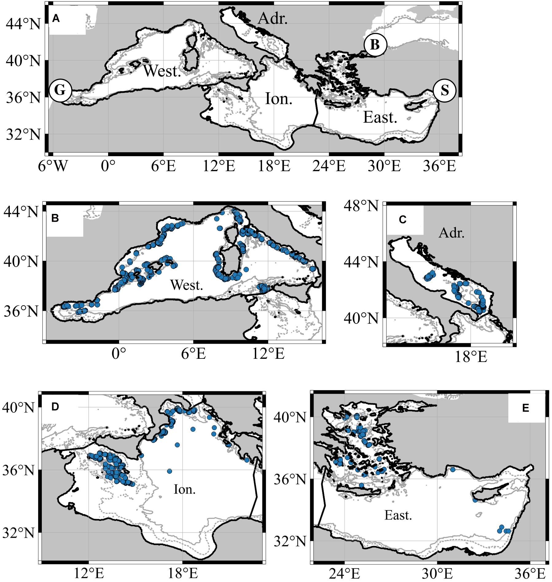
Figure 1. (A) The Mediterranean Sea with the four main sub-regions (Western: West; Adriatic: Adri, Ionian: Ion and Eastern: East) and flow exchanges with the Atlantic Ocean [Gibraltar Strait (G)]; the Red Sea [Suez Canal (S)], and the Black Sea [Bosporus Strait (B)]. Panels (B–E) represent sampling sites per sub-region. Isobath of 200 m (dashed line) and 1000 m (continuous line) are also represented.

The basin is heterogeneous with shallow sub-regions like the Adriatic Sea (mean depth around 300 m, Figure 1) and deep ones like the Ionian and Levantine seas (depths between 2500 and 4000 m; Zavatarelli and Melor, 1995; Durrieu de Madron et al., 2011). Decreasing gradients of nutrient and productivity are observed from north to south and west to east, making the Mediterranean Sea one of the most oligotrophic areas of the world ocean (Danovaro et al., 2010). Opposite trends are observed for temperature and salinity with increasing values eastward. In the twilight layer (i.e., mesopelagic and deeper layers) of the basin, temperature and salinity values are higher than in any other ocean (Gorlov, 2009). In the mesopelagic layer, there are longitudinal gradients of temperature and salinity, which correspond to 13°C and 38.4 PSU in the western basin and 15.5°C and 39.1 PSU in the eastern basin (Zavatarelli and Melor, 1995). This enclosed sea, despite covering only 0.32% of the world ocean volume, is an area known for its endemic biodiversity hotspot, hosting 7–10% of the world’s marine biodiversity (Bianchi and Morri, 2000; Coll et al., 2010).

Data

Biomass of Mesopelagic Fish

We built a database of georeferenced mesopelagic fish biomass (t/km²) using data from peer-reviewed articles and/or scientific reports (Figure 1 and Supplementary Table 1). The database was constructed following a framework to account for differences in recorded data (e.g., abundance vs. biomass data); the details are provided in the Supplementary Materials). We only considered the biomass of adults or juveniles, excluding thus mesopelagic fish larvae. Selected deep-sea species consisted of species defined by FishBase (Froese and Pauly, 2015) either as mesopelagic or in some cases, as bathypelagic fishes. Even if bathypelagic fish usually live in waters deeper than the mesopelagic layer, some species occur in both mesopelagic and bathypelagic layers (e.g., Arctozenus risso: 0 to 2200 m depth) or are sometimes described as meso- and bathypelagic species by FishBase. In our study, we excluded bathypelagic species estimates if those species were not described as migrators to the mesopelagic layer. Overall, we extracted 11,430 mesopelagic fish biomass estimates for the period 1994–2011 that were collected either during day or night or both (Supplementary Table 1). Thirteen mesopelagic families were collected with Myctophidae and Sternoptychidae representing 70% of the total biomass. We then tested the diurnal and seasonal effect on the biomass data and excluded this effect from model formulation because of their non-significance in explaining data variability (F(1,402) = 0.1346; p > 0.05, F(4,1952) = 2.16; p > 0.05, respectively).

Sampling stations were mainly distributed along the slope of the Mediterranean Sea (Figure 1) and 49.7% of them were in the Western sub-region. An overview description of this database is presented in Supplementary Table 1 of the Supplementary Information. To finally keep one biomass value per station and year, mesopelagic fish biomass of the different collected species was summed up, which reduced the database to 2,694 records.

Environmental Predictors

Environmental data were used to predict the distribution of mesopelagic fish biomass in space and time. We used yearly gridded environmental data from a three-dimensional hydrodynamic biogeochemical model (GETM-MedERGOM) covering the whole Mediterranean Sea at a spatial resolution of 0.083° (Macias et al., 2013, 2014a, 2015). Detailed description and validation of this model can be found in Macias et al. (2013). Environmental predictors were selected based on their potential to influence mesopelagic fish distribution: primary production (PPR) (Olivar et al., 2012); dissolved oxygen (DO) (Kinzer et al., 1993), seawater salinity (S), seawater temperature (T) (Themelis, 1997; Danovaro et al., 2004).

Environmental predictors were averaged for salinity, temperature, and DO and integrated for the PPR over three depth layers:

0–10 m depth layer (i.e., surface):

0–150 m depth layer (i.e., the euphotic zone also delimited by the Mixed Layer Depth)

0–1000 m depth layer (i.e., the entire water column where mesopelagic fish might occur).

This was done to understand the influence/importance of selected depth related environmental data in the estimation of the biomass and distribution of mesopelagic fish.

Also, to consider sub-regional differences in environmental and biological characteristics of the region, georeferenced biomasses were linked to the four main Mediterranean sub-regions (i.e., Western, Adriatic, Ionian, and Eastern) following the division as provided by the Marine Strategy Framework Directive (MSFD; 2008/56/EC).

Statistical Methods and Set Up

Generalized Additive Model

Generalized additive model is a non-parametric regression method that uses a link function to establish a relationship between the response variable and a “smoothed” function of the explanatory variable(s) (Hastie and Tibshirani, 1986). The strength of GAM is its ability to deal with highly non-linear and non-monotonic relationships between the response and the set of explanatory variables. Here, we used GAM to estimate the mesopelagic fish biomass in function of selected environmental predictors following the equations:

if Layer = 0–10 m:

where s and poly stand for smooth functions, Layer the depth-layer considered and Sub-region, one of the four sub-regions dividing the Mediterranean Sea and ε the residuals. The residuals ε were assumed to follow a Gaussian distribution.

To deal with spatial autocorrelation, we assess the residuals correlation structure using the exponential correlation structure (ECS). In the ECS, the correlation σ between two observations is given by:

where d is the distance between the two observations and r is the range (corresponding to the distance at which the residuals are no longer correlate). Longitude and latitude are projected in ETRS-LAEA (also called ETRS 89) for the calculation of the d and r of the residuals’ correlation structure in metric units. The ECS is chosen between the Gaussian, spherical and linear correlation, based on the reduction of the Akaike’s information criterion (AIC). The optimal combination of the predictor variables is performed by comparing nested models using the likelihood ratio test with maximum likelihood estimation (Zuur et al., 2007). To validate the model, we randomly split the data into training (2/3) and validation (1/3), we then compared the predictions of both models (training/validation) and once considered suitable, we used the entire data set to predict the biomass of mesopelagic fish. The best model was chosen based on (1) the lowest AIC and (2) significant covariates (Wood, 2001). Here, GAM was run using the “mgcv” package (version 1.8-7) in R.

Random Forest

Random forest is an ensemble of decision trees based on a bootstrap aggregation method (also called bagging method; see Breiman, 1996), which partitions the variable of interest, here, biomass, from decisions made on the predictor data. RF is a statistical model, which has been increasingly used in ecological modeling to predict fish biomass with the lowest errors (Knudby et al., 2010). As for GAM, RF can deal effectively with non-linearity between predictors and the response variable (Breiman, 2001). To tune the algorithm, the model requires two parameters: the number of regression trees, ntree and the number of different predictors tested at each split, mtry. Prior to the growth of each tree, one-third of the dataset, called the Out-Of-Bag (OOB), is excluded from the bootstrap and used for cross-validation. Decision trees are built by splitting the other two-thirds of the dataset according to four randomly selected predictors. The algorithm of RF looks for the optimal values (e.g., a value that reduces the variance) of these predictors before the splits. Once the decision trees are built, the accuracy of the tree predictions is assessed by using the observed biomass from the OOB dataset. In our study, we decided to set mtry to 2 and ntree to 500 to optimize the time computation and avoid errors in predictions (Breiman, 2001). We then estimated the mesopelagic fish biomass by averaging the predictions obtained from the 500 decision trees. To be consistent with GAM, RF used the same set of environmental predictors. RF was implemented using the “randomForest” package (version 4.6-10) in R, which is based on an algorithm described by Breiman (2001).

Models Performance

Generalized additive model and RF performances were compared through data variability explained by the models (i.e., cross-validated R² in RF and deviance in GAM) and the importance of environmental predictors (i.e., the reduction in deviance in GAM and the increase rate of the mean square error in RF). In GAM, the reduction in deviance is calculated as the difference between residual deviance of the final model and the residual deviance of a model where one or more predictors are dropped. In RF, the increase rate of the mean square error is obtained excluding one predictor from the model.

In addition to these methods, we decided to run (100 times) both models with a 10-fold cross-validation technique. The root-mean-square-error (RMSE) obtained through the 10-fold cross-validation was used to summarize the errors and compare the two statistical methods (the one yielding the lowest RMSE was the model with a better fit). RMSE was estimated as follow:

with n, the total number of data, y_i the i-th prediction and y_i the i-th observation.

Density Estimates in Space and Time

Once calibrated and validated, the best RF and GAM models were selected to predict the mesopelagic fish biomass (t/km²) in space and time for the period 1994–2011 using the spatially explicit and time-resolved environmental variables provided by the hydrodynamic-biogeochemical model. Taking into consideration that mesopelagic fish occur mainly in waters deeper than 200 m, we discarded all the predictions estimated over a topography shallower than 200 m. For both models and each depth layer, we calculated the arithmetic average of the estimated biomass for the entire Mediterranean Sea and for each sub-region (Western, Adriatic, Ionian, and Eastern). Additionally, we estimated biomass trends and spatial distributions using a geometric average over the period 1994–2011.

Finally, we tested the sensitivities of the models to changes in catchability, an input parameter that was used to estimate the mesopelagic biomass in the dataset (see Supplementary Materials for details). Both selected models were trained and run with catchability values ranging between 0.05 and 0.35, which were the values of catchabilities observed in the available scientific literature.

Results

Model Performances

The most statistically significant results were obtained with RF. This model, in fact, explained between 27.0 and 28.4% the variance of the data depending on the depth layer considered (Table 1); hypotheses on the residuals were analyzed and verified (Supplementary Figures 1–3 in Supplementary Information). As for GAM, the deviances ranged between 14.9 and 15.4% with smooth functions statistically significant (p-values < 0.05) and analysis on residuals verified (Supplementary Figures 4–6 in Supplementary Information). Bathymetry was the most important predictor for both models followed by salinity, temperature, and PPR for RF and by DO, PPR, and salinity for GAM (Table 1).

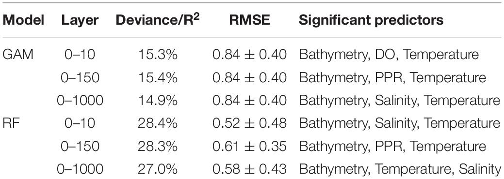
Table 1. Performances of the GAM and RF models by depth layer. Model performance is measured by the R² and RMSE.

Based on the RMSE from the 10-fold cross-validation analysis, the performances of RF were generally better than the ones from GAM, with an average of 0.57 and 0.84, respectively (Table 1).

In both models, the first two layers (0–10 and 0–150 m) contributed the most to the total explained variance. In GAM, the environmental predictors from the depth layer 0–150 m showed the highest improvement while in RF this was observed for the depth layer 0–10 m. For these GAM and RF models, the marginal effects of the environmental predictors in common (i.e., bathymetry, temperature, and salinity) on the biomass showed similar patterns (Supplementary Figures 7, 8).

Model-Estimated Mesopelagic Fish Biomass

The predicted mesopelagic fish biomass differed considerably between models. The average estimate obtained for the whole time period (1994–2011) and for the entire basin was 1.08 t/km² with GAM and 0.10 t/km² with RF. As for changes in catchability, GAM and RF showed a variance in modeled average biomass of around 220 and 280% when catchability decreased to 0.05 and −51% and −54% when it increased to 0.35 (Supplementary Figure 9), respectively.

Sub-Regions

High differences were observed between the two methods even at sub-regional scale (Figure 2). Overall, in RF there was a clear decreasing gradient of mesopelagic biomass from West to East while in GAM, such pattern was more homogenous. In GAM, the Ionian Sea was the sub-region with the highest densities with an average estimated at 1.77 t/km² and estimates were contained in the 95% confidence interval from 0.01 to 5.80 t/km². In RF, the highest values were found in the Western sub-region and averaged at 0.22 t/km². The 95% confidence interval for that sub-region included values from 0.01 to 0.66 t/km². For both GAM and RF models, the Adriatic sub-regions had low estimates of biomass (i.e., <0.06 t/km²). Then, the Ionian and Eastern sub-regions had the highest discrepancy rates (i.e., biomasses from GAM were ∼130 times higher than those estimated by RF).

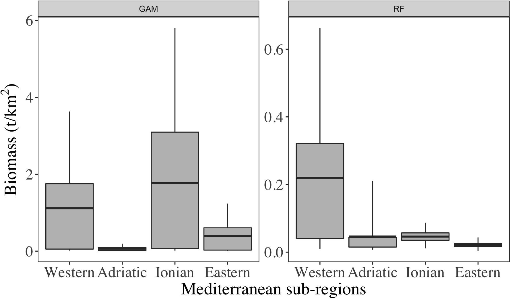
Figure 2. Statistics of biomass predicted using GAM (A) and RF (B) models by sub-regions of the Mediterranean Sea. The value ranges are from the 5th to the 95th quantiles.

Spatial Distribution and Temporal Dynamics

Spatial differences between the two models were mainly detected looking at the biomass distributions over the bathymetry (Figure 3). In general, small biomass estimates (<0.03 t/km²) were observed in all the sub-regions, particularly near the continental shelves and had low value variations (Supplementary Figure 10). On the contrary, the highest estimates (>3.5 t/km², Figure 3A) in GAM were encountered over the deep areas of the Western Mediterranean Sea, the Ionian and Eastern sub-regions (Figure 3). In those areas where the average estimates were high and the data coverage was absent, we also observed high standard deviation (i.e., from 0.4 to 3.5 t/km²) of the prediction (Supplementary Figure 10A). Similarly, but with values 10 times smaller, biomass estimates in RF were high (>0.4 t/km², Figure 3B) in the deep areas of the Western Mediterranean Sea. Nonetheless, the standard deviation was relatively the highest (from 0.4 to 1.9 t/km²) near Spanish islands and the Sicilia Strait in the Western Mediterranean Sea.

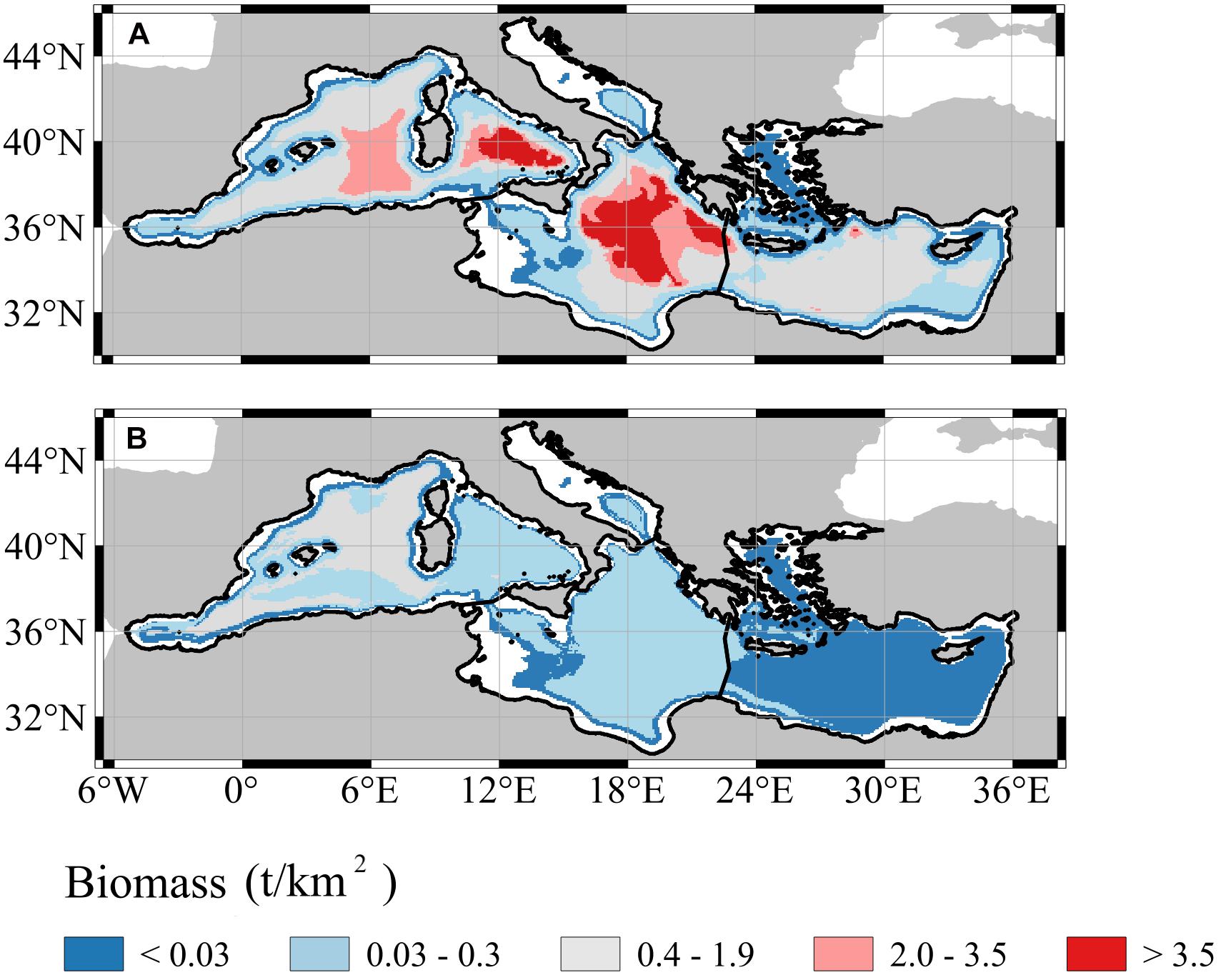
Figure 3. Spatial distribution of mesopelagic fish biomass averaged over the whole time period (1994–2012) using GAM (A) and RF (B). White areas correspond to the topography shallower than 200 m which was discarded from the analysis.

Temporal dynamics estimated by both models for the whole Mediterranean Sea suggested an increase of total mesopelagic fish biomass from 1995, which then decreased softly until 2007 before to rose steeply again in GAM (Figure 4). Meanwhile, in RF, the total mesopelagic biomass declined in 1998 and remained stable throughout 2001 and 2011. Similar trends were observed at sub-regional scale (Supplementary Figure 11), with the exception of the Ionian sub-regions in RF where the decline was not pronounced as in the other sub-regions. The temporal dynamic pattern in GAM was mainly driven by the temporal variability observed in the Ionian sub-region (Supplementary Figure 11C), where the predicted biomass was the highest (see Figure 2) while it was the Western sub-region influencing the most the modeled values in RF (Supplementary Figures 10, 11A). Temporal trends showed that RF was able to capture the decline of mesopelagic fish as observed in the sampling data (Figure 4) for the end of 1990s while GAM showed only a fluctuation.

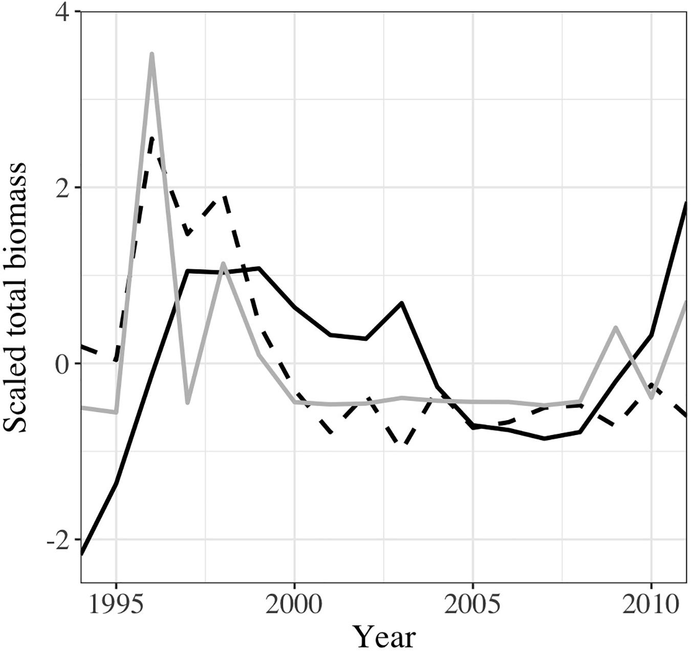
Figure 4. Interannual variability of the predicted mesopelagic fish biomass in the Mediterranean Sea using GAM (continuous line), and RF (dashed line) compared to the observed mesopelagic fish biomass as provided by our dataset (gray line). The biomass was scaled (subtraction of the average then division by the standard deviation) to facilitate the comparison.

Discussion

Data Quality and Model Performance

This study provides a first spatial and temporal estimate of mesopelagic fish biomass in the Mediterranean Sea. It covers the last two decades and is based on the best available data and best available modeling tools. Yet, we acknowledge that considerable gaps still exist, particularly with regards to data quality. For instance, environmental data were extracted from a hydrodynamic-biogeochemical model that, despite being tested and validated, still show levels of uncertainties. This particular model set-up has been shown to properly represent past (Macias et al., 2014a), present (Macias et al., 2014b), and future (Macias et al., 2015) conditions in this semi-enclosed basin, although it is still far from a perfect description of environmental characteristics. As a particle example of model limitations, it could be mentioned the underestimation of primary production values in certain particular areas such as along the Egyptian Coast, on the Tunisian continental shelf and in the shallow Adriatic waters, which are known to be highly productive (Bosc et al., 2004). Using time series from survey data (instead of modeled climatological data) could possibly result in a better model performance; however, data at regional scale with appropriate spatial and temporal coverage are inexistent.

The extraction of mesopelagic fish biomass estimates from scientific literature can itself be a considerable source of bias. Indeed, in some cases, mesopelagic biomass was obtained from studies where the scope was generally not aimed at targeting mesopelagic fish. Lack of regional data impedes a proper analysis of the dynamics of mesopelagic fish in the region. Besides, it also hampers the development of a comprehensive ecosystem analysis to evaluate the functional role of these fish in the food web. More efforts should be dedicated to improve data collection and quality in the region. Sampling data should be more homogeneously distributed in space and should have a better time coverage. Nonetheless, the biomass database that was constructed for this study followed a rigorous approach (Supplementary Materials) using, when missing, data (weights from length-weight relationships) coming from FishBase (a global biodiversity information system on finfishes)¹. We use this system to gather consistent information among the different studies and species, and to reduce further noise coming from information collected in localized/individual studies. Yet, we acknowledge that FishBase has limitations, particularly associated to uncertainties on the ecology of many mesopelagic fish species; thus, further efforts should be made to reduce this knowledge gap.

Probably the most uncertain parameter of our biomass database is the catchability that was fixed at 0.16 (i.e., only 16% of mesopelagic fishes in the volume swept by the trawl gear(s) were assumed to be caught by the gear), to estimate the biomass present in the water column, across species and surveys. This catchability was estimated by averaging published catchabilities of different gears [i.e., 6 feet Isaac Kidd Midwater Trawl (Barkley, 1964, 1972); Engel 152 (May and Blaber, 1989)], which were also the main gears used to sample mesopelagic fish biomass in the Mediterranean Sea. Such value might have led to under- or overestimate of the mesopelagic fish biomass. Catchability is a matter of fish size, fish species, fishing depth and a lot of other parameters, which makes it difficult to measure and estimate. Unfortunately, at the time this research was undertaken, no more information was available to fill these gaps. The results obtained from the sensitivity analysis, which tested different catchabilities, showed that biomass values may vary greatly depending on the catchability used. This result reinforces the need to conduct further research on catchability to reduce the uncertainties associated to the mesopelagic fish biomass estimation.

Lastly, our sampling sites were located close to the coast or the continental shelf and mainly in the northern part of the Mediterranean Sea. Spatial autocorrelation was not detected in the residuals of the two models. However, due to the scarcity of biomass sampling data for open waters, the estimation of the mesopelagic fish biomass distribution could be biased. In fact, with a better distribution of the sampling, we could undoubtedly improve the patterns of some relationship between biomass and predictors (e.g., Supplementary Figures 7, 8) and for the spatial estimation of the biomass (e.g., Figure 3). Nevertheless, the estimation of biomass on the continental slope of the Mediterranean Sea is in line with existing knowledge. The increase of biomass with bathymetry was previously observed by Moranta et al. (2004) and Massutí and Reñones (2005), and high estimation above the continental slope is expected since those zones shelter a high biodiversity and food abundance (Danovaro et al., 2010).

With the run of two models, we were able to assess communalities and main differences in depicting the relationship of mesopelagic fish with its environment. Our results highlight a general different pattern among these tools, not only in the absolute biomass estimates but also in the temporal and spatial distribution. These two models are commonly used to assess species distributions in both marine and terrestrial realms (e.g., Moisen et al., 2006; Rooper et al., 2017; Kosicki, 2020), however RF models have been seen to have substantially more performance power and control over the model overfitting compared to GAM approaches (Elith et al., 2006; Rooper et al., 2017), as it is also shown in this study. This is likely because of the RF algorithm, which is an ensemble of models (regression trees), each built on a random selection of relatively few predictors (Breiman, 2001). Besides, contrary to the GAM approaches, the RF algorithm did not seem to overestimate the biomass at places where we originally lacked data.

In addition, the statistically significant differences in predictive performance between these two modeling tools, suggest the need for further comparative studies, including other techniques and model types, to get stronger and more reliable conclusions (Martínez-Minaya et al., 2018). It has been observed that these statistical tools, together with machine learning methods, have great potential in reducing prediction error while incorporating non-linear and interaction effects (Knudby et al., 2010). As pointed out by several studies (Fulton, 2010; Piroddi et al., 2017), there is “no one best model” but rather a suite of tools should be examined given the high uncertainty associated to the questions that such approaches aim to address.

Estimates of Biomass

The distribution of biomass over the whole Mediterranean Sea and the relationship with some environmental predictors had comparable patterns with the available literature. First, our predicted biomass with GAM for the whole region was of the same order of magnitude as estimated by Gjøsaeter and Kawaguchi (1980), which was ∼3 t/km² for the entire region. On the other hand, RF was more in agreement with Gjøsaeter and Kawaguchi (1980) in relation to the distribution of mesopelagic biomass which was higher in the western Mediterranean Sea compared to the eastern part. This is also in line with other studies in the Mediterranean Sea that suggest a decreasing gradient of species richness from west to east (Danovaro et al., 2010; Piroddi et al., 2017) due to an increased oligotrophy in the eastern regions. Since our study is the first of its kind in producing spatiotemporal maps and trends of mesopelagic fish biomass for the basin, unfortunately, at this stage, no further and clear conclusions can be drawn. A hypothesis could be associated to an increase in water temperature in the basin that together with low levels of primary production, typical of the oligotrophic nature of the Mediterranean Sea might have created unfavorable conditions for mesopelagic fish biomass to thrive in the eastern region.

In this study, bottom depth was the variable that explained the greatest portion of the biomass and spatial distribution of mesopelagic fish. Many studies have demonstrated the importance of this parameter on the distribution of reef and demersal fish (Knudby et al., 2010; Pham et al., 2015), and it is not surprising that even deeper fish like mesopelagic fish are as well highly influenced by this variable. Having environmental data from a 3D hydrodynamic biogeochemical model allowed us to explore the influence of different depth related environmental data on the dynamics of mesopelagic fish. Our results showed no significant variations among the three assessed depth layers, suggesting an important contribution of each of these compartments in the pattern of these fish. Yet, our study indicated that the euphotic zone was the area with the highest influence on the distribution and abundance of mesopelagic fish. These results might be biased by the survey data used in this assessment, which was mainly collected close to coastal/shelf areas. Further studies should better evaluate this aspect when/if more data (in open waters) become available. The use of spatially explicit environmental variables from hydrodynamic-biogeochemical models, extracted as in this case at different depths, highlighted the importance of considering such tools to better capture fish dynamics and their linkage with the environment (Piroddi et al., 2017, 2020).

Biomass could also be linked to other parameters we did not consider in this study, notably those of species-dependent character. We think particularly of an increase in natural mortality or a modification of certain biological features e.g., growth (smaller sizes) and reproduction (less survival of larvae; Herring, 2002) with environmental changes. We did not consider the rate of by-catch from the fishing activities, but it might be important when looking at mesopelagic fish biomass trend. Even if mesopelagic fish are not targeted by any commercial fisheries, they are discarded at a considerable scale in such fisheries (Gorelli et al., 2016).

Conclusion and Perspectives

This study constitutes the first attempt to estimate the biomass and the spatial temporal patterns of mesopelagic fish using environmental variables as predictors. Compared to the work of our predecessors, Gjøsaeter and Kawaguchi (1980), this work provides a first preliminary estimate of the mesopelagic fish biomass for the whole Mediterranean Sea (not only the Western and Eastern sub-basins), and for more recent years (while the previous estimates were for the 1980s). Most importantly, this is the first study that assesses potential trends and spatial-temporal maps of this group of fish in the region. We agree that there is still considerable uncertainty associated to data availability and quality and model results, but our study aims to provide a baseline for assessing future mesopelagic fish biomass and distribution in the Mediterranean Sea. The two well-established statistical models used to estimate spatially and temporally mesopelagic fish biomass distribution in the Mediterranean Sea showed different results in relation to the distribution and the variation of the mesopelagic fish biomass in the region. Our analysis indicate that RF was the model that gave best biological results and acceptable performance. Finally, we believe that in order to improve our understanding in the processes behind mesopelagic fish dynamics in the Mediterranean Sea, more tools and analyses with integrated regional data should be tested.

Data Availability Statement

The raw data supporting the conclusions of this article will be made available by the authors, without undue reservation.

Author Contributions

MC-H gathered materials, built models, carried out post-analyses, wrote the manuscript. CP conceived the manuscript concept, supervised the first author, gathered materials, revised the manuscript. FQ built models, revised the manuscript. DM provided the material, revised the manuscript. VC conceived the manuscript concept, supervised the first author, gave access to materials, revised the manuscript. All authors contributed to the article and approved the submitted version.

Conflict of Interest

The authors declare that the research was conducted in the absence of any commercial or financial relationships that could be construed as a potential conflict of interest.

The handling editor declared a past co-authorship with one of the authors CP.

Acknowledgments

We thank the two reviewers for their very helpful comments, which have helped to improve the paper. VC acknowledges support through Natural Science and Engineering Research Council of Canada (NSERC) Discovery Grant RGPIN-2019-04901.

Supplementary Material

The Supplementary Material for this article can be found online at: https://www.frontiersin.org/articles/10.3389/fmars.2020.573986/full#supplementary-material

Footnotes

1. ^ www.fishbase.org

References

Barkley, R. (1964). The theoretical effectiveness of towed-net samplers as related to sampler size and to swimming speed of organisms. J. Cons. 29, 146–157. doi: 10.1093/icesjms/29.2.146
Barrett, R. T., Anker-Nilssen, T., Gabrielsen, G. W., and Chapdelaine, G. (2002). Food consumption by seabirds in Norwegian waters. ICES J. Mar. Sci. 59, 43–57. doi: 10.1006/jmsc.2001.1145
Bernal, A., Olivar, M. P., Maynou, F., Fernández, and de Puelles, M. L. (2015). Diet and feeding strategies of mesopelagic fishes in the western Mediterranean. Prog. Oceanogr. 135, 1–17. doi: 10.1016/j.pocean.2015.03.005
Bianchi, C. N., and Morri, C. (2000). Marine biodiversity of the Mediterranean Sea: situation, problems and prospects for future research. Mar. Pollution Bull. 40, 367–376. doi: 10.1016/s0025-326x(00)00027-8
Bosc, E., Bricaud, A., and Antoine, D. (2004). Seasonnal and interannual variability in algal biomass and primary production in the Mediterranean Sea as derived from 4 years of SeaWIFS observations. Glob. Biogeochem. Cycles 18:17. doi: 10.1029/2003GB002034
Coll, M., Piroddi, C., Steenbeek, J., Kaschner, K., Rais Lasram, F. B., Aguzzi, J., et al. (2010). The Biodiversity of the Mediterranean Sea: Estimates. Patterns, and Threats. PLoS One 5:e11842. doi: 10.1371/journal.pone.0011842
Cotter, J. (2009). A selection of nonparametric statistical methods for assessing trends in trawl survey indicators as part of an ecosystem approach to fisheries management (EAFM). Aquat. Living Resour. 22, 173–185. doi: 10.1051/alr/2009019
Danovaro, R., Company, J. B., Corinaldesi, C., et al. (2010). Deep sea biodiversity in the Mediterranean Sea: The known, the unknown and the unknowable. PLoS One 5:e11832. doi: 10.1371/journal.pone.0011832
Danovaro, R., Dell’Anno, A., and Pusceddu, A. (2004). Biodiversity response to climate change in a warm deep sea. Ecol. Lett. 7, 821–828. doi: 10.111/j.1461-0248.2004.00634.x
Davison, P. C., Koslow, J. A., and Kloser, R. J. (2015). Acoustic biomass estimation of mesopelagic fish: backscattering from individuals, populations, and communities. ICES J. Mar. Sci. 72, 1413–1424. doi: 10.1093/icesjms/fsv023
Demirel, N., Zengin, M., and Ulman, A. (2020). First large-scale eastern mediterranean and black sea stock assessment reveals a dramatic decline. Front. Mar. Sci. 7. doi: 10.3389/fmars.2020.00103
Dornan, T., Fielding, S., Saunders, R. A., and Genner Martin, J. (2019). Swimbladder morphology masks Southern Ocean mesopelagic fish biomass. Proc. R. Soc. B. 286:0353. doi: 10.1098/rspb.2019.0353
Durrieu de Madron, X., Guieu, C., Sempéré, R., Conan, P., Cossa, D., et al. (2011). Marine ecosystems’ responses to climatic and anthropogenic forcings in the Mediterranean. Prog. Oceanogr. 91, 97–166. doi: 10.1016/j.pocean.2011.02.003
Elith, J., Graham, C. H., Anderson, R. P., Dudík, M., Ferrier, S., Guisan, A., et al. (2006). Novel methods improve prediction of species’ distributions from occurrence data. Ecography 29, 129–151. doi: 10.1111/j.2006.0906-7590.04596.x
Escobar-Flores, P. C., O’Driscoll, R. L., Monthomery, J. C., Ladroit, Y., and Jendersie, S. (2020). Estimates of density of mesopelagic fish in the Southern Ocean derived from bulk acoustic data collected by ships of opportunity. Polar Biol. 43, 43–61. doi: 10.1007/s00300-019-02611-3
Ferretti, F., Myers, R. A., Serena, F., and Lotze, H. K. (2008). Loss of Large Predatory Sharks from the Mediterranean Sea. Conserv. Biol. 22, 952–964. doi: 10.1111/j.1523-1739.2008.00938.x
Freer, J. J., Tarling, G. A., Collins, M. A., Partridge, J. C., and Genner, M. J. (2019). Predicting future distributions of lanternfish, a significant ecological resource within the Southern Ocean. Divers Distrib. 25, 1259–1272. doi: 10.1111/ddi.12934
Fulton, E. (2010). Approaches to end-to-end ecosystem models. J. Mar. Syst. 81, 171–183. doi: 10.1016/j.jmarsys.2009.12.012
Giménez, J., Marçalo, A., García-Polo, M., García-Barón, I., Castillo, J. J., Fernández-Maldonado, C., et al. (2017). Feeding ecology of Mediterranean common dolphins: The importance of mesopelagic fish in the diet of an endangered subpopulation. Mar. Mammal Sci. 34, 136–154. doi: 10.1111/mms.12442
Gjøsaeter, J., and Kawaguchi, K. (1980). A Review of the World Resources of Mesopelagic Fish. Rome: Food And Agriculture Organization Of The United Nations.
Gorelli, G., Blanco, M., Sardà, F., Carreton, M., and Company, J. B. (2016). Spatio-temporal variability of discards in the fishery of the deep-sea red shrimp Aristeus antennatus in the northwestern Mediterranean Sea: implications for management. Scientia Mar. 80, 79–88.
Gorlov, A. A. (2009). “Temperature Differences in the Ocean at Low Latitude and Between Sea or River Water and Air at High Latitudes,” in Renewable Energy Sources Charged With Energy from the Sun and Originated from Earth-Moon Interactions, ed. E. E. Shpilrain (Abu Dhab: EOLSS Publishers Company Limited).
IPBES (2016). “The methodological assessment report on scenarios and models of biodiversity and ecosystem services,” in Secretariat of the Intergovernmental Science-Policy Platform on Biodiversity and Ecosystem Services, eds S. Ferrier, K. N. Ninan, P. Leadley, R. Alkemade, L. A. Acosta, H. R. Akçakaya, et al. (Bonn: IPBES).
Irigoien, X., Klevjer, T. A., Røstad, A., Martinez, U., Boyra, G., Acuña, J. L., et al. (2014). Large mesopelagic fishes biomass and trophic efficiency in the open ocean. Nat. Commun. 5:4271. doi: 10.1038/ncomms4271
Jennings, S., and Collingridge, K. (2015). Predicting Consumer Biomass, Size-Structure, Production, Catch Potential, Responses to Fishing and Associated Uncertainties in the World’s Marine Ecosystems. PLoS One 10:e0133794. doi: 10.1371/journal.pone.0133794
Kaartvedt, S., Staby, A., and Aksnes, D. (2012). Efficient trawl avoidance by mesopelagic fishes causes large underestimation of their biomass. Mar. Ecol. Prog. Ser. 456, 1–6. doi: 10.3354/meps09785
Kaiser, M. J., Attrill, M. J., Jennings, S., Thomas, D. N., Barnes, D. K. A., Brierley, S. A., et al. (2011). Marine ecology: processes, systems, and impacts. Oxford: Oxford University Press.
Katsanevakis, S., Coll, M., Piroddi, C., Steenbeek, J., Ben Rais, Lasram, F., et al. (2014). Invading the Mediterranean Sea: biodiversity patterns shaped by human activities. Front. Mar. Sci. 1:32. doi: 10.3389/fmars.2014.00032
Kinzer, J., Böttger-Schnack, R., and Schulz, K. (1993). Aspects of horizontal distribution and diet of myctophid fish in the Arabian Sea with reference to the deep water oxygen deficiency. Deep Sea Res. Part II: Topical Stud. Oceanogr. 40, 783–800. doi: 10.1016/0967-0645(93)90058-u
Knudby, A., Brenning, A., and LeDrew, E. (2010). New approaches to modelling fish–habitat relationships. Ecol. Model. 221, 503–511. doi: 10.1016/j.ecolmodel.2009.11.008
Kosicki, J. Z. (2020). Generalised Additive Models and Random Forest Approach as effective methods for predictive species density and functional species richness. Environ. Ecol. Stat. 27, 273–292. doi: 10.1007/s10651-020-00445-5
Littell, J. S., McKenzie, D., Kerns, B. K., Cushman, S., and Shaw, C. G. (2011). Managing uncertainty in climate-driven ecological models to inform adaptation to climate change. Ecosphere 2:102. doi: 10.1890/ES11-00114.1
Loots, C., Koubbi, P., and Duhamel, G. (2007). Habitat modelling of Electrona antarctica (Myctophidae, Pisces) in Kerguelen by generalized additive models and geographic information systems. Polar Biol. 30, 951–959. doi: 10.1007/s00300-007-0253-7
Lotze, H. K., Tittensor, D. P., Bryndum-Buchholz, A., Eddy, T. D., Cheung, W. W., Galbraith, E. D., et al. (2019). Global ensemble projections reveal trophic amplification of ocean biomass declines with climate change. Proc. Natl. Acad. Sci. 116, 12907–12912.
Macias, D. M., Garcia-Gorriz, E., and Stips, A. (2015). Productivity changes in the Mediterranean Sea for the twenty-first century in response to changes in the regional atmospheric forcing. Front. Mar.Sci. 2:79. doi: 10.3389/fmars.2015.00079
Macias, D., Garcia-Gorriz, E., and Stips, A. (2013). Understanding the causes of recent warming of mediterranean waters. How much could be attributed to climate change? PLoS One 8:e81591. doi: 10.1371/journal.pone.0081591
Macias, D., Garcia-Gorriz, E., Piroddi, C., and Stips, A. (2014a). Biogeochemical control of marine productivity in the Mediterranean Sea during the last 50 years. Glob. Biogeochem. Cycles 28, 897–907. doi: 10.1002/2014GB004846
Macias, D., Stips, A., and Garcia-Gorriz, E. (2014b). The relevance of deep chlorophyll maximum in the open Mediterranean Sea evaluated through 3D hydrodynamic-biogeochemical coupled simulations. Ecol. Model. 281, 26–37. doi: 10.1016/j.ecolmodel.2014.03.002
Mann, K. H. (1984). “Fish production in open ocean ecosystems,” in Flows of energy and materials in marine ecosystems: theory and practice, ed. M. J. R. Fasham (New York, NY: Plenum Press), 435–458. doi: 10.1007/978-1-4757-0387-0_17
Martínez-Minaya, J., Cameletti, M., Conesa, D., and Pennino, M. G. (2018). Species distribution modelling: a statistical review with focus in spatio-temporal issues. Stochastic Environ. Res. Risk Assess. 32, 3227–3244. doi: 10.1007/s00477-018-1548-7
Massutí, E., and Reñones, O. (2005). Demersal resource assemblages in the trawl fishing grounds off the Balearic Islands (western Mediterranean). Sci. Mar. 69, 167–181. doi: 10.3989/scimar.2005.69n1167
May, J. L., and Blaber, S. J. M. (1989). Benthic and pelagic fish biomass of the upper continental-slope off eastern Tasmania. Mar. Biol. 101, 11–25. doi: 10.1007/bf00393474
Moisen, G. G., Freeman, E. A., Blackard, J. A., Frescino, T. S., Zimmermann, N. E., and Edwards, T. C. (2006). Predicting tree species presence and basal area in Utah: a comparison of stochastic gradient boosting, generalized additive models, and tree-based methods. Ecol. Model 199, 176–187. doi: 10.1016/j.ecolmodel.2006.05.021
Moranta, J., Palmer, M., Massuti, E., Stefanescu, C., and Morales-Nin, B. (2004). Body fish size tendencies within and among species in the deep-sea of the Western Mediterranean. Sci. Mar. 68(Suppl.3), 141–152. doi: 10.3989/scimar.2004.68s3141
Olivar, M. P., Bernal, A., Molí, B., Peña, M., Balbín, R., Castellón, A., et al. (2012). Vertical distribution, diversity and assemblages of mesopelagic fishes in the western Mediterranean. Deep Sea Res. Part I: Oceanogr. Res. Papers 62, 53–69. doi: 10.1016/j.dsr.2011.12.014
Pham, C. K., Vandeperre, F., Menezes, G., Porteiro, F., Isidro, E., and Morato, T. (2015). The importance of deep-sea vulnerable marine ecosystems for demersal fish in the Azores. Deep Sea Res. Part I: Oceanogr. Res. Papers 96, 80–88. doi: 10.1016/j.dsr.2014.11.004
Piroddi, C., Coll, M., Liquete, C., Macias, D., Greer, K., Buszowski, J., et al. (2017). Historical changes of the Mediterranean Sea ecosystem: modelling the role and impact of primary productivity and fisheries changes over time. Sci. Reports 7:44491. doi: 10.1038/srep44491
Piroddi, C., Coll, M., Steenbeek, J., Macias-Moy, D., and Christensen, V. (2015). Modelling the Mediterranean marine ecosystem: addressing the challenge of complexity. Mar. Ecol. Prog. Series 533, 47–65. doi: 10.3354/meps11387
Piroddi, C., Colloca, F., and Tsikliras, A. C. (2020). The living marine resources in the Mediterranean Sea Large Marine Ecosystem. Environ. Develop. 2020:100555. doi: 10.1016/j.envdev.2020.100555
Rooper, C. N., Zimmermann, M., and Prescott, M. M. (2017). Comparison of modeling methods to predict the spatial distribution of deep-sea coral and sponge in the Gulf of Alaska. Deep-sea Res. Part I 126, 148–161. doi: 10.1016/j.dsr.2017.07.002
Salvanes, A. G., and Kristoffersen, J. B. (2001). Mesopelagic fish0Cambridge: Academic Press. 1711–1717. doi: 10.1006/rwos.2001.0012
Saunders, R. A., Fielding, S., Thorpe, S. E., and Tarling, G. A. (2013). School characteristics of mesopelagic fish at South Georgia. Deep Sea Res. Part I: Oceanogr. Res. Papers 81, 62–77. doi: 10.1016/j.dsr.2013.07.007
Saunders, R. A., Hill, S. L., Tarling, G. A., and Murphy, E. J. (2019). Myctophid Fish (Family Myctophidae) Are Central Consumers in the Food Web of the Scotia Sea (Southern Ocean). Front. Mar. Sci. 6:530. doi: 10.3389/fmars.2019.00530
Themelis, D. E. (1997). Variations in the abundance and distribution of mesopelagic fishes in the Slope Sea off Atlantic Canada. Halifax, NS: Doctorate of Philosophy, Dalhousie University.
Valinassab, T., Pierce, G. J., and Johannesson, K. (2007). Lantern fish (Benthosema pterotum) resources as a target for commercial exploitation in the Oman Sea. J. Appl. Ichthyol. 23, 573–577. doi: 10.1111/j.1439-0426.2007.01034.x
Williams, A., Koslow, J. A., Terauds, A., and Haskard, K. (2001). Feeding ecology of five fishes from the mid-slope micronekton community off southern Tasmania. Australia. Mar. Biol. 139, 1177–1192. doi: 10.1007/s002270100671
Wilson, R. W., Millero, F. J., Taylor, J. R., Walsh, P. J., Christensen, V., Jennings, S., et al. (2009). Contribution of Fish to the Marine Inorganic Carbon Cycle. Science 323, 359–362. doi: 10.1126/science.1157972
Wood, S. N. (2001). mgcv: GAMs and generalized ridge regression for R. R News 1.Amsterdam: Elsevier.
Würtz, M. (2010). Mediterranean Pelagic Habitat. Oceanographic and Biological Processes, An Overview. Gland: IUCN.
Zavatarelli, M., and Melor, G. L. (1995). A numerical study of the Mediterranean Sea Circulation. J. Phys. Oceanogr. 25, 1384–1414. doi: 10.1175/1520-0485(1995)025<1384:ansotm>2.0.co;2
Keywords: generalized additive model, Random Forest, spatial model, Mediterranean Sea, biomass distribution, mesopelagic fish
Citation: Clavel-Henry M, Piroddi C, Quattrocchi F, Macias D and Christensen V (2020) Spatial Distribution and Abundance of Mesopelagic Fish Biomass in the Mediterranean Sea. Front. Mar. Sci. 7:573986. doi: 10.3389/fmars.2020.573986
Received: 18 June 2020; Accepted: 01 December 2020;
Published: 18 December 2020.
Edited by:
Stelios Katsanevakis, University of the Aegean, GreeceReviewed by:
Binduo Xu, Ocean University of China, ChinaRyan Alexander Saunders, British Antarctic Survey (BAS), United Kingdom
Copyright © 2020 Clavel-Henry, Piroddi, Quattrocchi, Macias and Christensen. This is an open-access article distributed under the terms of the Creative Commons Attribution License (CC BY). The use, distribution or reproduction in other forums is permitted, provided the original author(s) and the copyright owner(s) are credited and that the original publication in this journal is cited, in accordance with accepted academic practice. No use, distribution or reproduction is permitted which does not comply with these terms.
*Correspondence: Morane Clavel-Henry, mhenry.research@gmail.com; morane.clavel-henry@ucd.ie; Chiara Piroddi, chiara.piroddi@ec.europa.eu
†Present address: Diego Macias, Instituto de Ciencias Marinas de Andalucía (ICMAN), Consejo Superior de Investigaciones Científicas (CSIC), Madrid, Spain