Spatial Variation in Thermal Stress Experienced by Barnacles on Rocky Shores: The Interplay Between Geographic Variation, Tidal Cycles and Microhabitat Temperatures

Introduction

Global climate change has been predicted to severely impact marine ecosystems, driving mass mortality, altering selection pressures and the geographic distribution of species (Helmuth et al., 2006a; Hawkins et al., 2008). The rocky intertidal zone is an excellent model system to study and predict the effect of global warming in marine systems as, under natural tidal cycles, intertidal species experience daily variation in both air and seawater temperatures depending on their vertical position on the shore. Under the stress experienced during low tide emersion periods, species in the intertidal zone are considered to be living very close to their physiological tolerance limits and, thus, are especially sensitive to changing thermal environments (Helmuth et al., 2006a; Somero, 2010; Han et al., 2018).

A common prediction of the impacts of increasing temperature is a latitudinal, poleward shift of species with the assumption that thermal stress will be more intense toward the equator (Southward et al., 1995; Broitman et al., 2001; Helmuth et al., 2006a; Parmesan, 2006; Sanda et al., 2019). Helmuth et al. (2002), however, showed that estimates of the “body” temperature of the intertidal mussel, Mytilus californianus, using biomimetic robomussels, did not increase monotonically with decreasing latitude along the west coast of United States, but rather reflected a mosaic of sites with different thermal environments. Helmuth et al. (2002) attributed this mosaic pattern to spatial variation in timing of low tides in summer; as low tides at locations in higher latitudes mostly occurred during the day (when thermal stress is higher), whilst those at lower latitudes occurred predominantly during the night (also see Finke et al., 2007 for tide variations across continents). A further study on heat stress of limpets along the Atlantic coast of Europe, based on thermal profiles recorded by biomimetic loggers (robolimpets), also demonstrated that the degree of exposure to solar radiation may override large-scale latitudinal gradients in thermal stress, resulting in a mosaic pattern of hot and cold sites (Seabra et al., 2011).

The West Pacific (W Pacific) and the South China Sea is a global marine biodiversity hotspot which experiences complex climatic patterns, seasonal monsoons and strong ocean currents (Hu et al., 2000; Williams et al., 2019). In this region, despite indications that extreme hot days are becoming more frequent, whilst extreme cool days are decreasing (Lima and Wethey, 2012; Tsang et al., 2013), the relationship between environmental temperatures and the level of heat stress experienced by rocky intertidal species is poorly understood (but see Marshall et al., 2010). Understanding which major environmental factors affect the body temperature of intertidal species is, therefore, an important prerequisite to inform predictions of potential changes in the distribution and abundance of intertidal organisms in the W Pacific and the South China Sea (Hui et al., 2020).

Acorn barnacles of the genus Tetraclita are common ecosystem engineers on rocky shores of the W Pacific and South China Sea (Chan et al., 2007, 2008; Cartwright and Williams, 2012, 2014), forming dense beds in the mid to lower tidal levels. In Hong Kong, mid to high shore populations of Tetraclita japonica can experience body temperatures up to 45°C during summer low tides and, consequently, suffer high mortality rates (Chan and Williams, 2003; Chan et al., 2006; Wong et al., 2014). In laboratory experiments, 50% of T. japonica enter coma when they experience air temperatures of 40°C for 2 h (Wong et al., 2014). Time length between the two consecutive heat stress events can affect the recovery of barnacles from heat stress (Fraser and Chan, 2019). There are, however, limited records of short- and long-term natural variations in intertidal thermal environments from this region, and so relating laboratory measured species’ thermal limits to on-shore conditions is problematic (Williams et al., 2016). Recently, Chan et al. (2016) developed a biomimetic temperature logger (the “robobarnacle”) using Tetraclita shells and showed that temperatures recorded by these robobarnacles accurately reflect body temperatures of live Tetraclita barnacles on the shore. Body temperature of Tetraclita barnacles during summer low tides are often 4–5°C higher than air temperatures. Measuring air temperature may not be a reliable proxy for estimating body temperature of intertidal species (also see Marshall et al., 2010). Biomimetic temperature loggers can, therefore, record long-term and fine-scale temperature trajectories of intertidal species (see also Lima and Wethey, 2009). In the present study, Tetraclita robobarnacles were deployed to measure temperatures at different tidal heights and shore aspects at sites along a latitudinal gradient, spanning 13–25° latitude, from Taiwan to Hong Kong and Thailand. We aimed to (1) record the maximum, estimated body temperatures on Tetraclita barnacles using robobarnacles along the latitudinal gradient from Taiwan, Hong Kong and Thailand to investigate whether patterns showed a latitudinal monotonic trend, or were spatially variable representing a mosaic pattern; (2) compare the observed patterns of thermal environments in the W Pacific and South China Sea with latitudinal patterns of their Atlantic counterparts, (3) examine the latitudinal variation in frequency occurrence of thermal stress, and (4) examine the spatial variation in time length between stress events which will have implications on the effective length of recovery of the barnacles after stress. Using a combination of these approaches our goal was to determine the relative importance of regional vs. microhabitat environmental drivers of the body temperatures of sessile intertidal organisms on the W. Pacific and South China Sea.

Materials and Methods

Study Sites and Design

Measurements were made in Taiwan, Hong Kong and Thailand in hot seasons (see Williams et al., 2019) between June and September 2013 (Figure 1 and Supplementary Table S1). The latitudinal gradients throughout Taiwan, Hong Kong and Thailand cover several marine physical systems with distinct climate and hydrodynamic conditions. Two sites, Guei-Hao and Shen-Ao-Keng, were selected to represent the northern (N) and northeastern (NE) coasts of Taiwan (Figure 1), which are under the influence of the East China Sea system, climate is highly affected by NE monsoon winds during winter (Williams et al., 2019). Two sites, Shi-Ti-Ping and Jia-Ler-Shui were selected on the eastern (E) and southern (S) coasts of Taiwan (Figure 1), which are under the influence of the warm Kuroshio Current flowing northwards from the Philippines and are relatively warm, with smaller seasonal variation. Penghu Island (P) was selected to represent the western coast of Taiwan, which is under the influence of the Taiwan Strait system, characterized by a seasonal shift of the warm South China Sea current from the south and the cold China Coastal waters from the north (see Chan and Lee, 2012; Figure 1 and Supplementary Table S1). Hong Kong is located on the southern China coast and its waters are influenced by seasonal variation in currents from the Taiwan Strait, the Kuroshio Current and the South China Sea Warm Current (Williams et al., 2019). Three sites, Shek O (SO), Chung Hum Kok (CHK), and Middle Bay (MB) were selected on the south east, more oceanic coast of Hong Kong Island (Figure 1). Finally, one site at Si Chang Island, Thailand (Thai) was established in the Gulf of Thailand, which experiences slight seasonal variation in seawater temperature but a strong monsoonal climate with wet and dry monsoonal influences (Samakraman et al., 2009).

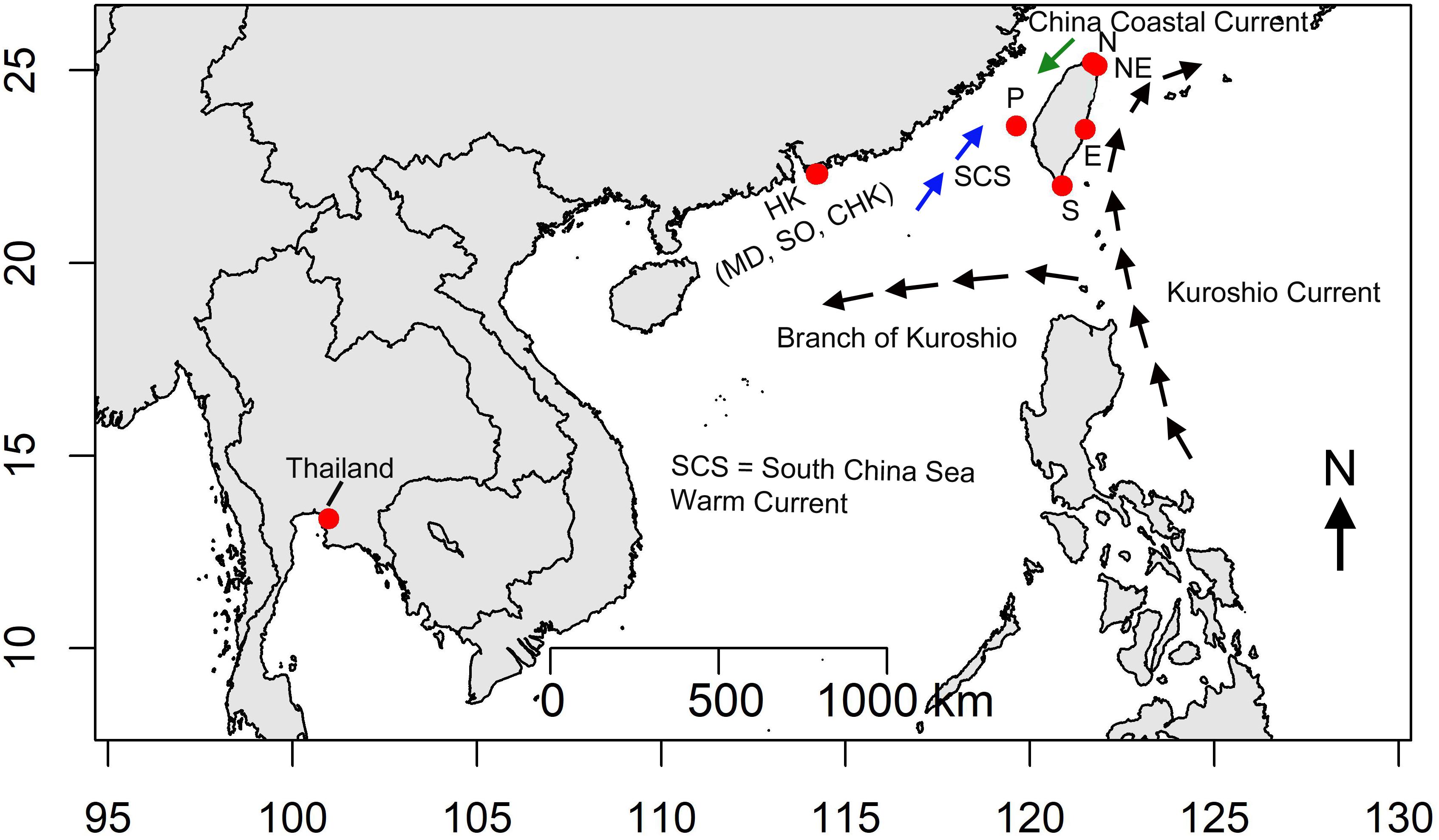
Figure 1. Study area, red dots indicate sampling sites. Sites in Taiwan (N – Guei-Hao, NE –Shen-Ao-Keng, E – Shi-Ti-Ping, S – Jia-Ler-Shui, P – Penghu, Hong Kong: MD – Middle Bay, CHK – Chung Hum Kok, SO – Shek O, Thailand – Si Chang Island). Black arrows indicate the flow of the Kuroshio from the Philippines to Japan, and the branch of the Kuroshio entering the South China Sea. The blue arrows indicate the South China Sea Current; and green arrows indicate the China Coastal Current.

Deployment of Robobarnacles

Robobarnacles were made from shells (>30 mm basal diameter) of Tetraclita japonica following Chan et al. (2016). The difference between the temperature recorded in robobarnacles and adjacent live barnacles was <1°C (Chan et al., 2016). Detailed measurements of local scale variation in thermal stress were made in Taiwan. At each site in Taiwan, two 10 m × 1 m areas of rocky shore, one east and one west facing, were selected. East-facing areas received solar radiation in the morning and west-facing areas during the afternoon. For each area, we monitored three tidal heights: high (1.75 m above Chart Datum), mid (1.5 m above Chart Datum) and low shore (1.25 m above Chart Datum; Supplementary Table S1), covering the vertical range of Tetraclita. Four robobarnacles were deployed at each height (Σn at each site = 2 areas/aspects × 3 shore heights × 4 robobarnacles = 24 robobarnacles). To examine larger scale, latitudinal variation in temperature, robobarnacles were deployed in Hong Kong and Thailand using the same scheme on east-facing shores (Supplementary Table S1). Data was recorded at a resolution of 0.5°C, at 1 h intervals. Some robobarnacles were lost during deployment, so the final number of robobarnacles ranged from 18 to 22 among sites in Taiwan, 7 to 12 among sites in Hong Kong and 4 at Thailand (see Supplementary Table S1).

Environmental Data

Site-specific environmental data were obtained for all Taiwan sites, including hourly recordings of rainfall, air temperature, wind speed, wind direction, daily proportion of solar duration, solar radiation, and hourly tidal heights during July–September 2013 from the nearest coastal weather stations (i.e., within 4–10 km, Central Weather Bureau, Taiwan, Supplementary Figure S1 and Supplementary Table S2). Hourly environmental data including rainfall, air temperature and predicted tide heights, were obtained for Hong Kong from the Hong Kong Observatory, and for Thailand from the Thai National Observatory (Supplementary Table S2). Tidal height data for the Taiwan sites were based on the Taiwan Vertical Datum 2001 (abbreviated as TWVD 2001) located in Keelung, Taiwan (Satellite Survey Center, Dept. of Land Administration, M.O.I., Taiwan, available at: http://gps.moi.gov.tw/SSCenter/). Due to the differences in the reference points for tide heights among regions, it is difficult to compare tide heights directly. Consequently, we derived anomalies of tidal height for each site for subsequent analyses (i.e., tidal height anomalies = tidal height measures subtracted by the site-specific mean).

Analysis

Temporal and Spatial Variation in Robobarnacle Temperatures

Temporal patterns

Monthly distributions of temperatures recorded by robobarnacles (hereafter “robo-temperatures”) were right-skewed for all sites and months (Supplementary Figure S2). Consequently, we derived natural-log-transformed robo-temperatures (with improved data symmetry; Supplementary Figure S3), exploring the effects of month, day, and phase patterns (categorical factors, see below) on the transformed temperature with a multiple linear regression. Phase patterns consisted of four diurnal phases: 0:00–5:00 am (midnight), 6:00–11:00 am (morning), 12:00–17:00 pm (afternoon), and 18:00–23:00 (evening), based on the apparent four discrete diurnal patterns of robo-temperatures (Supplementary Figure S4).

We examined temporal variation in robo-temperatures at two spatial scales; firstly comparisons between east and west facing orientations from pooled data from all sites; and secondly across sites with eastern aspects. Because the comparison of robo-temperature time series (months and phases) are logger-position specific, these temporal temperature measurements are not independent. To account for the effect of potential temporal autocorrelation on the ANOVA tests, we adjusted the effective sample size using the Quenouille procedure (Quenouille, 1952; Lima and Wethey, 2012), where N_effective = N(1 - r)/(1 + r); N: sample size, r: lag-1 autocorrelation coefficient of the residuals. As the N_effective < N, this adjustment increases mean square errors, resulting in conservative significance tests for our models (see Lima and Wethey, 2012). For the models with significant temporal patterns (e.g., significant effects of month and phase), Tukey HSD tests were used to determine potential differences among months or phases.

Spatial patterns

To explore variation in average robo-temperatures between orientations (east vs. west facing areas), among three shore levels (low, mid, and high), and among sites we used data in July and Aug, when robo-temperature records were available for all sites. Site-specific biotic or physical habitat structure may influence intertidal temperatures, confounding the spatial effects on robo-temperatures. Consequently, we applied a linear mixed-effects model (LME), with orientation and shore levels as two fixed effects and site as a random effect using the lme4 and lmerTest packages in R (Bates et al., 2014)¹. We evaluated the strength of the fixed effects using the likelihood ratio test (Faraway, 2006). To evaluate the site effect, we fitted a multiple linear regression with all three spatial variables as fixed-effects predictors and log(robo-temperature) as the response and the Tukey HSD test to evaluate variation in robo-temperature with respect to each level of these spatial variables. Given the strong diurnal cycles (i.e., phases) of robo-temperatures (see Results), we applied these LME models to fit data of individual phases, determining whether the effects of orientations or shore levels were consistent with those based on the combined-phase data.

Frequency of Heat Stress Events

In laboratory experiments, Wong et al. (2014) showed that there were three discrete coma responses of Tetraclita japonica from Hong Kong to different durations of exposure (Figure 2). We fitted a broken-stick model to this dataset (Wong et al., 2014) to depict the dependence of coma on time of exposure (Figure 2). The model fit suggested no barnacles would enter coma after being exposed to 40°C for <1 h, whereas 50% of individuals would when exposed for 2 h (i.e., proportion of individuals in coma increases linearly with exposure time ranging between 1 and 3 h; y = −0.43 + 0.46x) and >90% when exposed for ≥3 h (Figure 2).

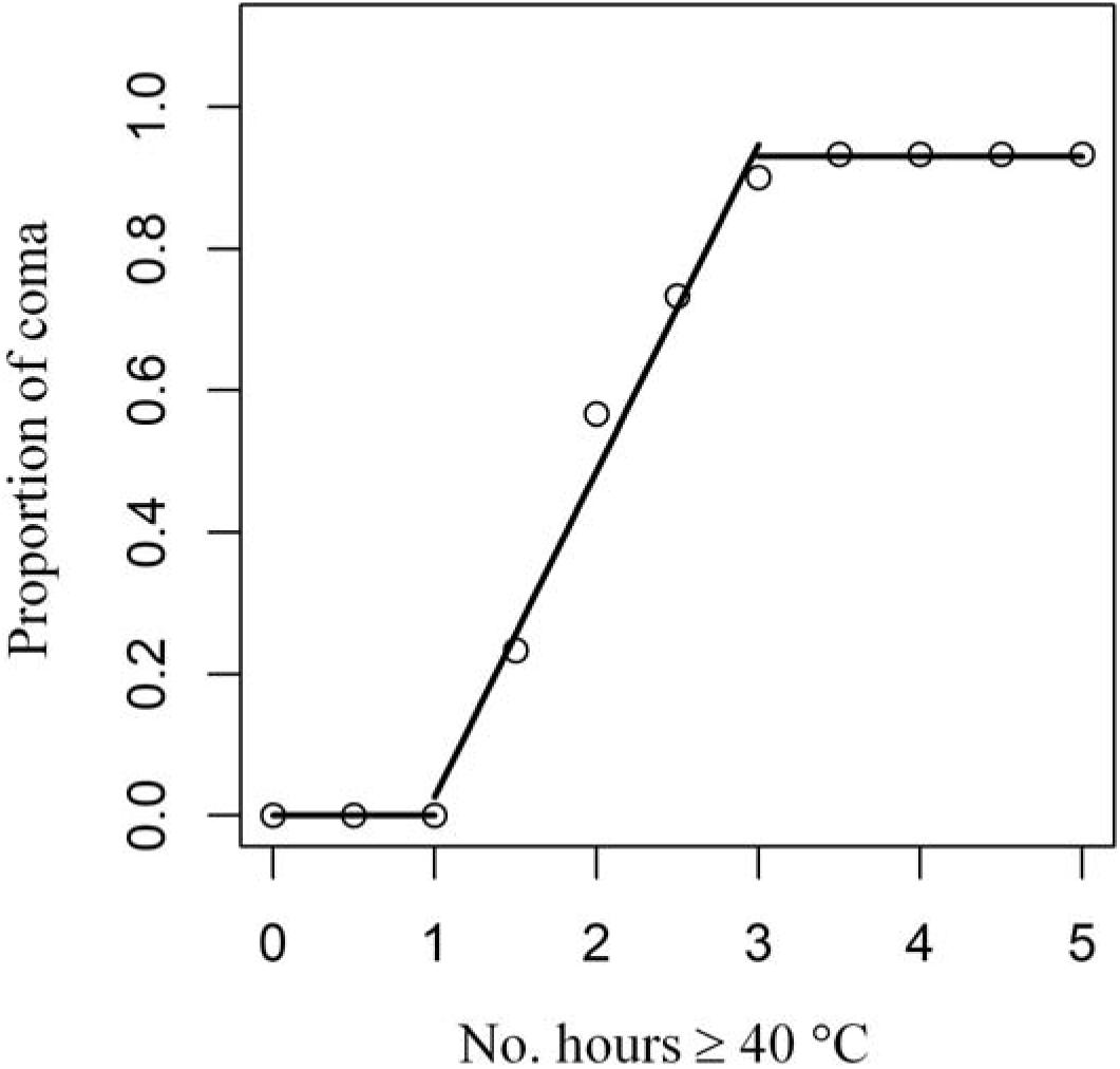
Figure 2. Broken-stick model fit of the experimental data of proportion of individuals in coma of the barnacle T. japonica as a function of the number of hours at 40°C (after Wong et al., 2014).

Given that the effects of heat stress depended on exposure time, we defined three levels of heat stress: low, intermediate, and high which denote when robobarnacles attained ≥40°C body temperature and were exposed to ≤1, 2 ≤ 3, and ≥3 consecutive hours at this temperature, respectively. We examined the frequency of occurrence of these levels by computing the monthly proportions of daily occurrence of these three levels of heat stress based on the east-facing habitats. We evaluated the effects of month, site, and shore on the proportions of hot season months when intermediate or high levels of heat stress occurred. The response variable was square-root transformed prior to regression fitting.

Variation in the “day intervals” between intermediate and high heat stress events provides an alternative index of the frequency of the three levels of heat stress. To explore spatial variation in the frequency of heat stress events, we estimated the intervals between incidences of intermediate and high levels of heat stress in July and August (the hottest months) for all shore levels and sites. We defined the intervals as number of days between two successive events of a given level of heat stress (i.e., an interval of 1 day denotes that heat stress of a given level occurs on 2 consecutive days, while a 2 day interval indicates that a given level of heat stress occurs on days 1 and 3, but not day 2). We excluded the last heat stress event in August and September. As the intervals were count estimates, we used a Poisson regression model with a log link to evaluate patterns of the intervals between the two levels of heat stress and among shores and sites. A Poisson regression assumes that the response variance is equal to its mean. When this assumption was violated (e.g., an overdispersion), we adjusted the P-values of the regression coefficients using the robust standard error (following Cameron and Trivedi, 1998). In addition, we fitted a negative binomial regression model as an alternative solution for violation of the assumption of Poisson regression. Multiple comparisons were conducted using the Tukey HSD test.

Relationship Between Environmental Conditions and Robo-Temperatures

The effects of air temperatures and tide heights on robo-temperatures for all sites were elucidated as these two variables are known to be important determinants of body temperatures for intertidal species (Helmuth et al., 2006b; Harley, 2008). For air temperature, we derived anomalies by centering site-specific hourly data by the site-specific mean; i.e., hourly values close to 0 indicate that the hourly data is similar to the mean, whereas positive and negative hourly values, respectively, represent values higher and lower than the mean. Then, we constructed the following LME model with anomalies of environmental variables, sites, and shore levels as fixed-effect predictors, and site as a random effect (i.e., random intercepts; Eq. 1):

Accounting for random variance of sites facilitates evaluating within-site responses of robo-temperatures to environmental variables. We used the likelihood ratio test to determine the significance of these fixed-effects variables. We also computed the constant e raised to a power of each of these regression coefficients, β₀ and β_5–12 of Eq. (1), to interpret variation in robo-temperatures among sites with no effects of environmental variable anomalies (hereafter referred to as “baseline robo-temperatures”). In order to compare the regression coefficients to interpret the effect of shore heights, we compared e^{β 0}, e^{β 3}, and e^{β 4} for among-shore differences in baseline robo-temperatures independent of the effects of environmental variables. Climate models (e.g., Intergovernmental Panel on Climate Change [IPCC], 2007, under the RCP6.0 scenario; also see New et al., 2011) predict that, on average, air temperatures in the W Pacific and South China Sea will warm by 1°C by the end of the twenty-first century. To explore the effects of environmental anomalies among sites, we derived the mean robo-temperature of each site given an 1°C increase in air temperature [i.e., exp((β₀ and β_5–12) + 1^∗(β₁ and β₁+β_13–20))] or a 10 cm increase in tidal height [i.e., exp((β₀ and β_5–12) + 10^∗(β₂ and β₂+β_21–28))]. Likewise, we compared the effects of environmental anomalies among shores by calculating the mean robo-temperature of each shore level given an 1°C increase in air temperature [i.e., exp((β₀ and β_3–4) + 1^∗(β₁ and β₁+β_29–30))] or a 10 cm increase in tidal height [i.e., exp((β₀ and β_3–4) + 10^∗(β₂ and β₂+β_31–32))]. We could not, however, compare the effects between these two environmental anomalies based on regression coefficients because they are scaled with different units.

Results

Monthly and Diurnal Variation

Robo-temperatures revealed pronounced variability (range = 23–48°C) and strong temporal trends (Table 1 and Supplementary Figure S2). Both site-specific and combined-sites analyses indicated that month and diurinal phase significantly affected robo-temperatures (Supplementary Table S3). Comparisons of the mean values of robo-temperatures revealed that the hottest months were July and August (Oct < May < Sept < June < July and Aug; Tukey’s HSD test see Supplementary Table S3) and the afternoon was the hottest phase (midnight < evening < morning < afternoon).

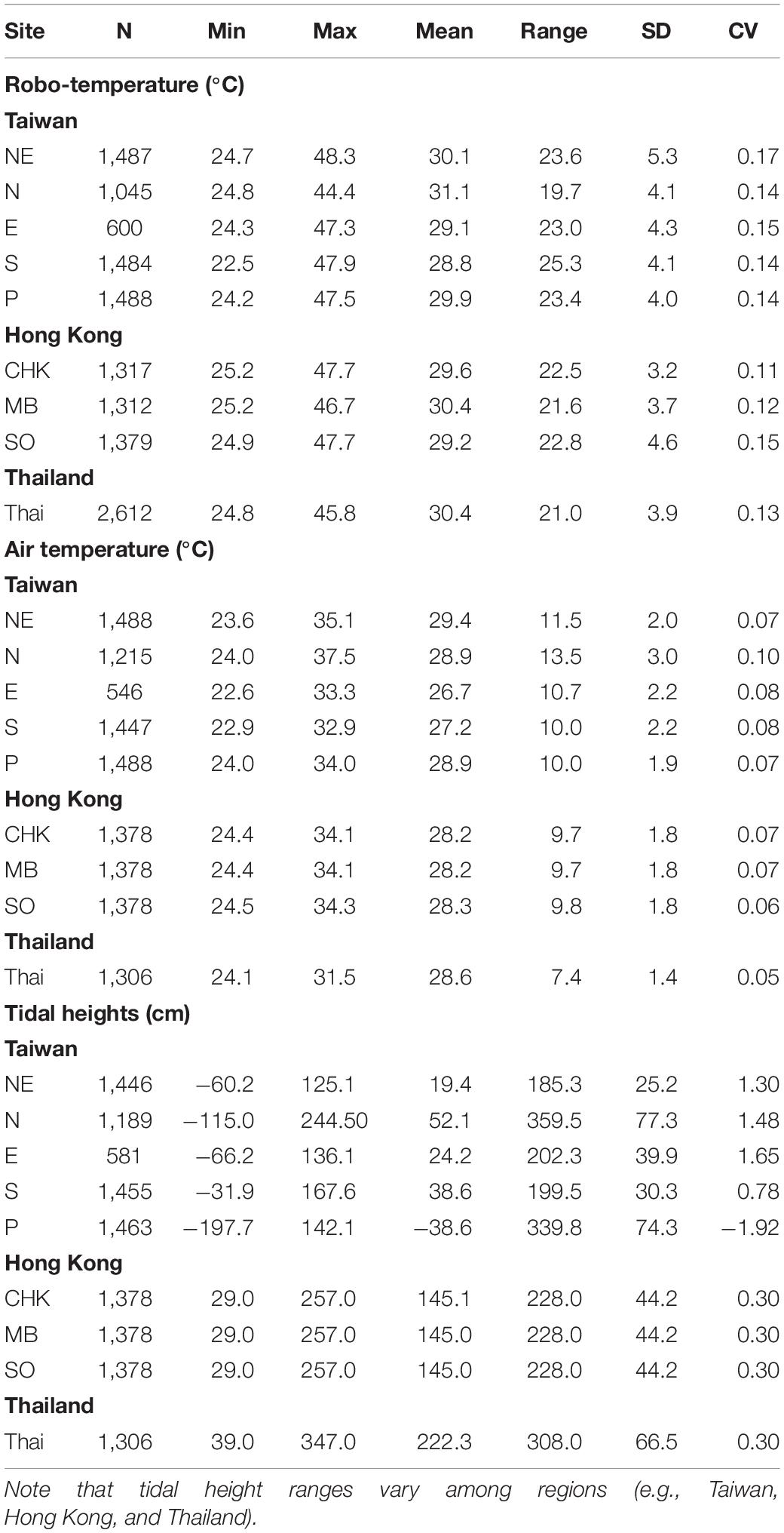
Table 1. Descriptive statistics (SD, Standard Deviation; CV, Coefficient of Variation) of robo-temperatures (°C), air temperature (°C), and tidal heights (cm) for various sites (for site abbreviations, refer to sections “Study Sites and Design” in Materials and Methods) in July and August (N = hourly data during the recording period).

Variation Between Aspects, Among Tidal Levels and Sites

Orientation did not have a significant effect on robo-temperature, but shore height did (P = 0.03; Tukey’s HSD test: low < mid < high Figure 3). Multiple linear regression revealed that robo-temperatures did not follow a latitudinal trend, with significant differences among sites with the highest robo-temperatures occurring at NE in Taiwan and Thailand; intermediate temperatures at SO (Hong Kong), N (Taiwan), P (Taiwan), and MB (Hong Kong); and the lowest at CHK in Hong Kong, E, and S Taiwan [with significant differences among these three sites; Tukey HSD test; Figure 3; note the ascending geographical latitudinal sequences of sites is: N, NE, E, P, S, HK (MD, CHK, SO) and Thailand, see Figure 1].

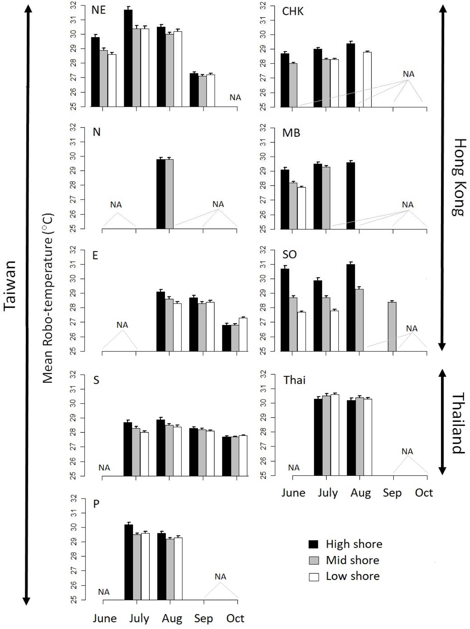
Figure 3. Barplots of monthly mean robo-temperatures of the sites with easterly aspects at three shore heights: high, mid, and low. Error bars represent SE. NA indicates sites/heights where data are unavailable.

The spatial patterns of robo-temperatures were, generally, not sensitive to phase changes. The effect of orientation, for example, was not significant in most phases, with the exception of morning (P for midnight = 0.43, morning = 0.03, afternoon = 0.26, and evening = 1), while the effect of shore was significant for most phases except in the evening (low < mid < high; P = 0.006, 0.03, 0.0001, and 0.19). In contrast, there were significant differences in robo-temperatures among phases at all sites [P < 0.001 for each of the four phases, (midnight < evening < morning < afternoon)].

Frequency of Occurrence of Heat Stress

The three levels (low, intermediate and high) of heat stress (i.e., ≤1, 2 ≤ 3, and ≥3 h of exposure at ≥40°C) varied between months and among shore levels and sites (Figure 4). Low levels of heat stress were most common at all shore levels (Figure 4 and Table 2). Intermediate and high heat stress levels, however, occurred more frequently at high as opposed to mid or low shore levels (1–3 x’s more frequent; Figure 4 and Table 2). Monthly patterns of heat stress also varied among sites (e.g., pronounced variation in the monthly proportions of heat stress at NE, but less so for the Hong Kong sites, Figure 4).

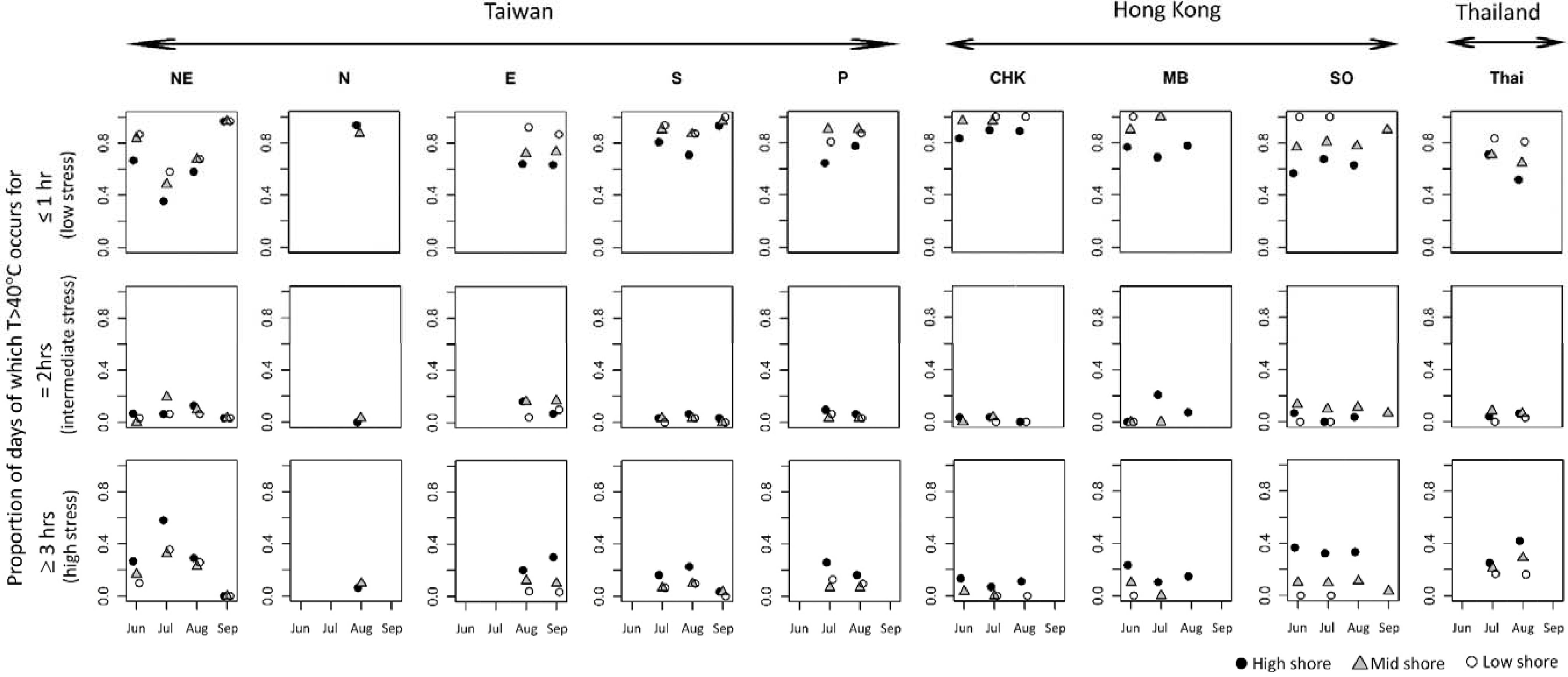
Figure 4. Proportions of monthly exposure to heat stress by location based on robo-temperature data. Top, middle, and bottom row, respectively, represents the proportions of exposure to low, intermediate, and high levels of heat stress (based on the broken-stick model fit to the dataset of Wong et al., 2014).

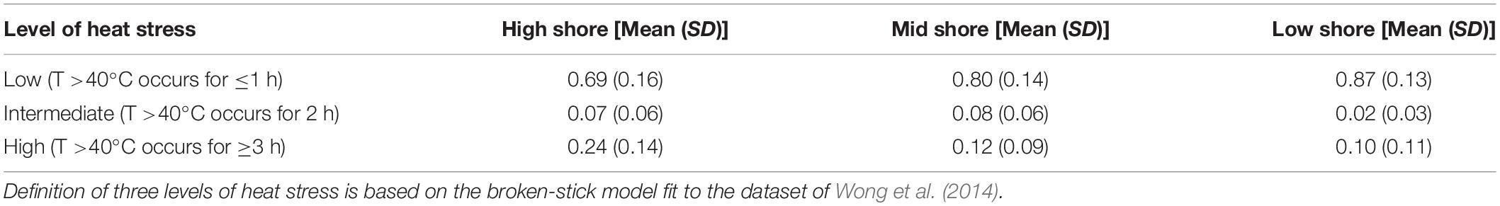
Table 2. Mean and standard deviation (SD) of proportion of days of three levels of heat stress at study locations in summer months (July and August).

Based on the robo-temperature data from east-facing habitats, the occurrence of intermediate levels of heat stress differed significantly among sites and shore levels (F = 3.59, df = 13, 49, P < 0.001, R² = 0.49; Figure 4) with intermediate heat stress occurring more frequently at the mid and high rather than the low shore levels (Tukey HSD tests P = 0.99, 0.02, and 0.03 for the comparisons of mid vs. high, high vs. low, and mid vs. low), and also varied significantly between Taiwan and Hong Kong; i.e., significant differences between CHK and NE and CHK and E, although other site pairs were similar (Tukey’s HSD tests, P = 0.05 and 0.002; Figure 4). No difference was observed for intermediate heat stress levels with month. All three variables, however, accounted for a significant proportion of the variance in levels of high heat stress (F = 7.24, df = 13, 49, P < 0.001, R² = 0.66; Figure 4). Frequencies of high heat stress increased from high shore as compared to mid and low shore (P < 0.05 for all pairwise comparisons in Tukey’s HSD). Significant differences in frequencies of high heat stress occurred between Thailand and NE (higher frequencies) vs. CHK, MB, and S (lower frequencies; Tukey HSD tests, P < 0.05; Figure 4). Also, high heat stress intensified significantly during June-Aug and weakened in September (Tukey HSD P < 0.001). Overall, robo-temperature data revealed that barnacles experienced intense heat stress at high shores across all study sites during the hot season months, but this varied with sites, with lower temperatures being recorded at CHK and MB in Hong Kong (Figure 4).

Intervals between heat stress events (which indicate low stress periods) varied between intermediate and high levels of heat stress and shore levels based on the robo-temperature data in July and Aug (Figure 5). Intervals between high heat stress events were right-skewed compared to being more evenly distributed between intermediate heat stress events (Figure 5). Poisson regression models indicated significant differences in the mean intervals between mid and high levels of heat stress, and among shore levels and sites (P ≤ 0.001). To account for overdispersion, a negative binomial regression model with the same response and predictors was run which showed consistent results with the Poisson model. Overall, both models indicated that mean intervals were greater for intermediate heat stress events (Figure 5), and varied with tidal height (low shore > mid shore > high shore for intermediate heat stress events and mid shore and low shore > high shore for high heat stress events, Figure 5). The among-site patterns of intervals of intermediate heat stress levels were less clear (Figure 6A), whereas intervals of high heat stress showed distinct geographic patterns, with shorter intervals occurring at high shore for the five sites of Taiwan and Thailand, and longer intervals at the sites of Hong Kong (Figure 6B).

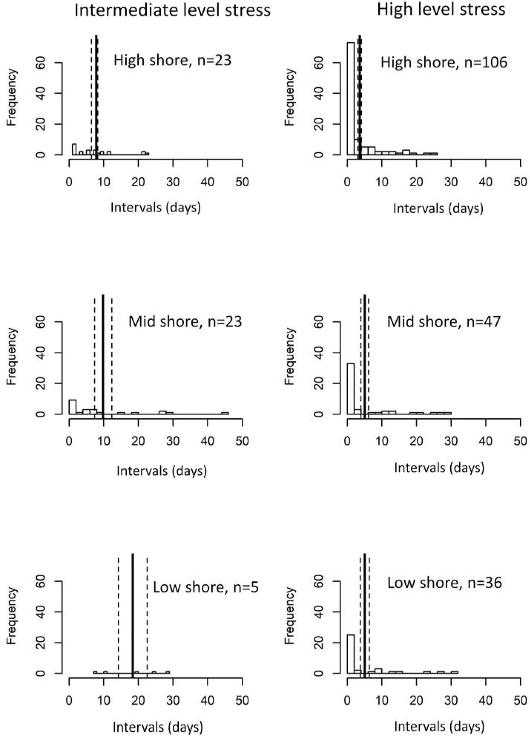
Figure 5. Distribution of time intervals between events of a given level of heat stress (left: intermediate level, right: high level) and by shore heights. Vertical solid and dashed lines denote mean ± 1 SE of the interval estimates (mean interval = 7.8, 9.8, and 18.4 days for high-, mid-, and low shore for intermediate-level heat stress; and 3.6, 5.1, and 5.1 days for high-, mid-, and low shore for high-level heat stress).

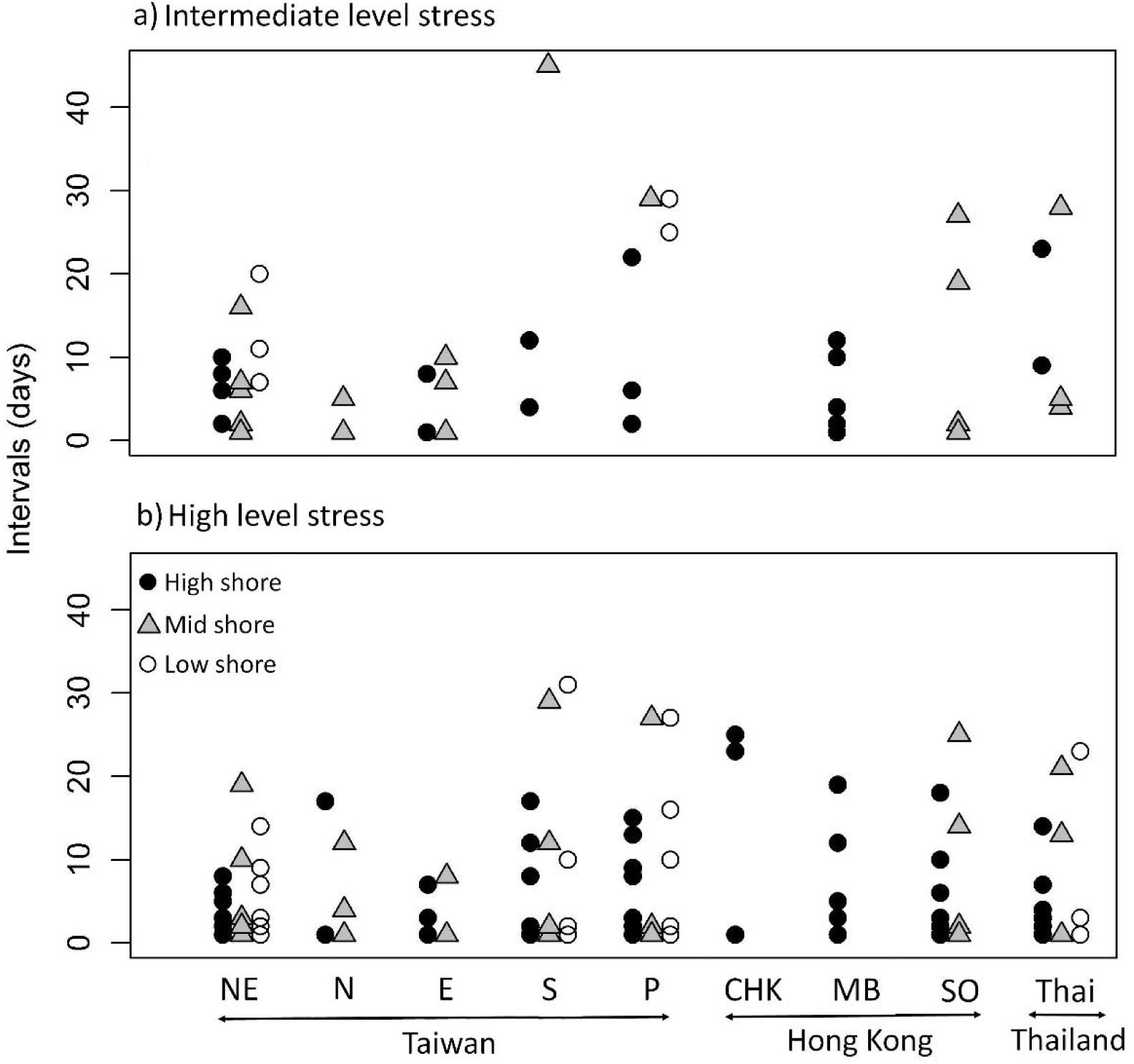
Figure 6. Scatter plots of intervals (days. i.e., period for recovery) between heat stress events (a: intermediate heat stress, b: high heat stress).

Effects of Environmental Conditions on Robo-Temperatures

Distributions of air temperatures and tidal heights were relatively symmetric, in contrast to those of wind speed, solar radiation, wind direction and robo-temperatures (Supplementary Figures S2, S5–S9). Based on the data of July–August for the Taiwan sites, the magnitudes of variation of air temperature were smaller than those of robo-temperatures (CV of air temperature < the CV of robo-temperature; Table 1), while the magnitudes of variation of tidal heights were greater than those of robo-temperatures (Table 1). There were positive correlations between air and robo-temperatures among locations (i.e., r = 0.54–0.63, P < 0.001).

The LME models [Eq. (1), based on data in July and Aug, east aspect, of all nine sites] showed pronounced variation in intercepts among sites, indicating differences in the baseline robo-temperatures among sites in the absence of anomalies of air temperature and tidal height (Figure 7A). The highest baseline robo-temperatures were found at NE in Taiwan and Thailand, whereas the lowest robo-temperatures occurred at CHK in Hong Kong (Figure 7A). The model fit showed significant interactions between sites and the anomalies of air temperatures and tidal height, indicative of variation in the influences of anomalies of either environmental variable among sites. A 1°C increment of anomalies would, for example, result in larger increases of baseline robo-temperatures at NE in Taiwan (+1.77°C) and Thailand (+1.60°C) but smaller increases at CHK in Hong Kong (+0.91°C; Figure 7A). The effects of anomalies of tide heights on robo-temperatures also varied among sites. An increase in tide heights of 10 cm would, for example, result in greater drops of robo-temperatures at NE (−0.55°C) and SO (−0.34°C) than N (−0.05°C; Figure 7A).

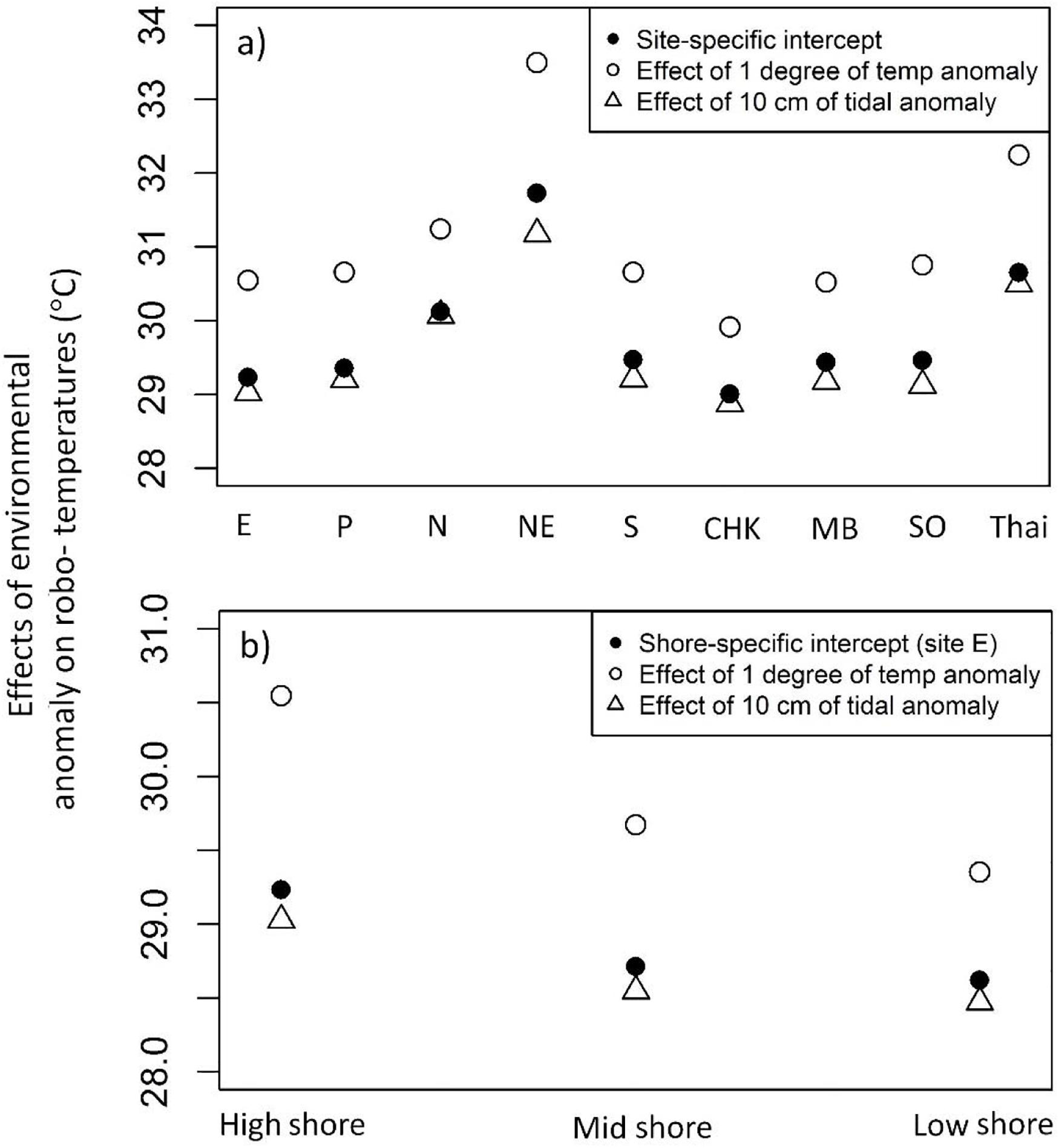
Figure 7. Estimates of robo-temperature at baseline (shown in solid black dots), rising 1°C (open circles), and rising 10 cm tidal height (open triangles). (a) Site-specific estimates; (b) Shore-specific estimates.

There were also significant interactions between shore levels and environmental anomalies, where an increase in 1°C anomalies resulted in differential increases of robo-temperatures among shore levels: high (+1.31°C), mid (+0.96°C), and low shore (+0.73°C; Figure 7B). Increasing tide heights by 10 cm resulted in decreasing of robo-temperatures along a gradient from high (−0.21°C), mid (−0.17°C), and low shore (−0.14°C; Figure 7B).

Discussion

Biomimetic loggers collecting long-term, high-resolution temperature data can provide a direct measure of temperature variability and extremes experienced by intertidal organisms during periods of high thermal stress such as in the summer/hot season (Helmuth et al., 2006b; Dong et al., 2015; Lathlean et al., 2015; Judge et al., 2018; this study). Based on such temperature data from robobarnacles, our analyses revealed a mosaic pattern of hot (e.g., NE of Taiwan and Thailand) and cool sites or “spots” (e.g., two Hong Kong sites CHK and MB) along locations of the W Pacific and South China Sea, which did not match a simple latitudinal pattern. The absence of a latitudinal gradient in the distribution of hot and cool spots is consistent with previous studies based on thermal profiles of robomussels (e.g., Helmuth et al., 2006b along the eastern Pacific) and robolimpets (e.g., Dong et al., 2015 in the Southern China; Seabra et al., 2011 along the Atlantic coast of Europe). While Helmuth et al. (2006b) found that the spatial heterogeneity in mussel temperatures could be explained by the timing of tidal inundations buffering the effects of air temperature along the Californian coastline, we found that hot spots in the W Pacific and South China Sea were characterized by frequent heat stress events (robo-temperatures ≥40°C for ≥2 h), but did not, however, always coincide with the maximum robo-temperatures recorded. The duration of the intervals between events of severe heat stress were, in general, correlated with the spatial patterns of heat stress (i.e., shorter intervals between heat events occurred at hot spots). The duration of the intervals between events of severe heat stress were, in general, correlated with the spatial patterns of heat stress (i.e., shorter intervals between heat events occurred at hot spots) which can be influenced by local weather conditions which are more stochastic events (i.e., logically, heat stress events only occur on sunny but not on cloudy days). The hot spot sites (NE of Taiwan and Thailand) are likely related to these sites which have more sunny days than other sites during the study period. Such results indicate that the intensity and frequency of latitudinal warming patterns interacts with weather conditions to have an additive effect on the thermal ecology of sessile intertidal organisms (see arguments in Helmuth et al., 2014). In the same manner, low stress periods (i.e., cloudy days), for example, may provide species time to recover from the physiological damages resulting from heat stress. Fraser and Chan (2019) showed that heat stress impacted the mating frequency and success of the intertidal barnacle, Fistulobalanus albicostatus, but a week of low heat stress allowed the barnacles to recover their mating frequencies, although these did not match pre-stressed levels. Seabra et al. (2016) also showed that Patella vulgata was able to recover from high temperatures experienced during low tide if allowed to re-immerse in cold water during high tide. The timing of low tides can also affect the heat stress experienced by intertidal species. Helmuth et al. (2002), for example, found that intertidal areas at higher latitudes experienced greater levels of stress as most of the low tides occur in daytime and vice versa at lower latitudes along the west coast of the United States. In the present study, the variation of the time of low tides along the latitudinal gradient from Taiwan to Thailand is relatively small, with low tides in Taiwan ∼1 h earlier than Thailand and ∼5 h earlier than Hong Kong (Supplementary Figure S10). When low tides in Taiwan occur in the afternoon, the low tides in Hong Kong are in the evening and, accordingly, Hong Kong shores experience relatively less thermal stress at these specific times than Taiwan.

In the present study, there was a strong correlation between hourly air temperatures and robo-temperatures. By plotting the relationship of robo-temperature vs. air temperature from all the sites (new Supplementary Figure S11), robo-temperature shows an almost ∼1:1 proportionally increase with low air temperatures (<30°C). However, at higher air temperatures (>30°C), the relationship between robo-temperature and air temperature showed increased variance suggesting air temperature, together with solar radiation and geothermal re-radiation (Marshall et al., 2010), are key components to drive the observed spatial variation in the robo-temperature. Solar radiation is naturally associated with sunny days which will affect the thermal environment of the whole intertidal area, as well as air temperatures. Importantly, the rock will absorb the solar radiation and re-emit it to the intertidal species (and also robobarnacles) which are in close contact with the rock surfaces. Accordingly, robo-temperatures are positively significantly correlated with both air temperature and solar radiation. Air temperature can, therefore, be a reliable predictor for patterns of body temperature of sessile intertidal species in the tropical and subtropical W Pacific and South China Sea. Our pattern is different to Marshall et al.’s (2010) findings in that the body temperature of the littorinid snail, Echinolittorina malaccana, in Brunei (4.5°N latitude) was primarily controlled by non-climatic sources of heat such as solar radiation and re-radiation from the substrate (i.e., not “climatically relevant” sources such as air temperatures). Interactions of local and regional effects may lead to different environmental drivers of body temperatures of intertidal organisms, for example, studies based on Eastern Pacific and European coastlines imply that environmental variables alone may not provide suitable predictive power to estimate the body temperatures of intertidal organisms. Helmuth (1998), for example, examined the effects of various environmental factors on the temperature of robomussels along the Eastern Pacific coast of Washington (48°N latitude) and concluded that no single environmental factor could alone account for the body temperature of mussels, and that air temperature was unlikely to be an accurate predictor of mussel body temperatures. In the Eastern Pacific and European Atlantic coast, shore aspect, which interacts with sun and shade, is important in affecting the body temperature and thermal stress of limpets (Seabra et al., 2011; Lima et al., 2016). Harley (2008) and Seabra et al. (2011) observed a marked difference in daily temperature maxima between north- and south-facing rock surfaces. In contrast to these studies, our results showed weak correspondence between robo-temperatures and substrate aspect (east vs. west). This discrepancy is probably because north facing rock surfaces in the Atlantic are often shaded (Seabra et al., 2011) and thus the relative importance of topographic shading to the thermal stress of intertidal species is much greater in the Eastern Pacific and European Atlantic region.

Robo-temperature data revealed that barnacles have higher body temperatures (maximum robo-temperatures ranging from 44 to 48°C) when compared to air temperatures 32–38°C (see also Chan et al., 2006). The water content of intertidal species is high and will be affected by heat sources from solar radiation, air temperatures and re-radiation from the rock substrate. As a result, body temperatures do not instantly equilibrate with air temperature (similar patterns have been recorded in the limpet Cellana grata in Hong Kong, Williams and Morritt, 1995 and in other gastropods by Vermeij, 1971).

Our analysis revealed that a 1°C increment in air temperature will result in severe thermal stress at certain locations (e.g., the hot spot locations by as much as 3.6 and 3.3°C at NE of Taiwan and Thailand) but relatively smaller body temperature changes at cool spots (e.g., 1.9°C at CHK in Hong Kong). Based on the maximum robo-temperature recorded in the present study, maximum estimated body temperature of barnacles in NE Taiwan (hot spots) can increase to 51.9°C (48.3 + 3.6 = 51.9) and body temperatures in CHK (cool spots) in Hong Kong up to 49.6 (47.7 + 1.9 = 49.6), respectively. Chan et al. (2006) recorded maximum body temperatures of high shore populations of Tetraclita at in Cape d’Aguilar in Hong Kong at ∼48°C and the majority of barnacles from this tidal level died off by the end of July–August. Thus it can be predicted that, in the future, individuals at today’s hot spots may experience body temperatures well beyond their current lethal temperatures and their populations may suffer heavy mortalities. Maximum body temperature for barnacles in present day cool spots will be around the current lethal temperature (∼48°C, Chan et al., 2006) under future increased air temperature based on the IPCC predictions. Whilst some populations in cool spots may, however, survive a 1°C increase in air temperature, there is, however, an interactive effect of temperature increase with shore level (e.g., a 2°C increase in air temperature will raise body temperatures by 2.7, 2.0, and 1.5°C at high, mid, and low shore levels, respectively). The observed variation in robo-temperatures among the three shore levels has clear implications for the future survival of barnacles settling at different shore heights (Connell, 1961; Appelbaum et al., 2002; Chan et al., 2006). As intertidal species live very close to their physiological tolerance limits (Helmuth et al., 2006a; Somero, 2012), our data suggest that under global warming, and without adaptive selection, it is likely that populations at high shore levels and located at present day hot spots may become locally extinct and the vertical distribution of species will, therefore, be altered which will have subsequent impacts on species interactions such as predation and competition lower on the shore (Helmuth et al., 2006b).

Data Availability Statement

The datasets generated for this study are available on request to the corresponding author.

Author Contributions

All authors designed and conducted the experiments. H-YW, BC, FL, RS, and GW conducted data analysis and wrote the manuscript.

Funding

BC acknowledges support from the Ministry of Science and Technology, Taiwan (MOST-103-2621-B-001-2005-MY3). FL was funded by FEDER through COMPETE (POCI-01-0145-FEDER-031088) and by National Funds through FCT (PTDC/BIA-BMA/31088/2017). RS was funded by FEDER through POR Norte (NORTE-01-0145-FEDER-031053) and by National Funds through FCT (PTDC/BIA-BMA/31053/2017).

Conflict of Interest

The authors declare that the research was conducted in the absence of any commercial or financial relationships that could be construed as a potential conflict of interest.

Supplementary Material

The Supplementary Material for this article can be found online at: https://www.frontiersin.org/articles/10.3389/fmars.2020.00553/full#supplementary-material

Footnotes

1. ^ www.r-project.org

References

Appelbaum, L., Achituv, Y., and Mokady, O. (2002). Speciation and the establishment of zonation in an intertidal barnacle: specific settlement vs. selection. Mol. Ecol. 11, 1731–1737. doi: 10.1046/j.1365-294X.2002.01560.x
Bates, D., Maechler, M., Bolker, B., and Walker, S. (2014). lme4: Linear Mixed-effects Models Using Eigen and S4. R Package Version 1.1-7.
Broitman, B. R., Navarrete, S., Smith, F., and Gaines, S. D. (2001). Geographic variation of southeastern Pacific intertidal communities. Mar. Ecol. Prog. Ser. 224, 21–34. doi: 10.3354/meps224021
Cameron, A., and Trivedi, P. (1998). Regression Analysis of Count Data. Cambridge: Cambridge University Press.
Cartwright, D. R., and Williams, G. A. (2012). Seasonal variation in utilization of biogenic microhabitats by littorinid snails on tropical rocky shores. Mar. Biol. 159, 2323–2332. doi: 10.1007/s00227-012-2017-3
Cartwright, D. R., and Williams, G. A. (2014). How hot for how long? The potential role of heat intensity and duration in moderating the beneficial effects of an ecosystem engineer on rocky shores. Mar. Biol. 161, 2097–2105. doi: 10.1007/s00227-014-2489-4
Chan, B. K. K., Akihisa, M., and Lee, P. F. (2008). Latitudinal gradient in the distribution of the intertidal acorn barnacles of the Tetraclita species complex (Crustacea: Cirripedia) in NW Pacific and SE Asian waters. Mar. Ecol. Prog. Ser. 362, 201–210. doi: 10.3354/meps07446
Chan, B. K. K., and Lee, P. F. (2012). “Biogeography of intertidal barnacles in different marine ecosystems of Taiwan – potential indicators of climate change?,” in Global Advances in Biogeography, ed. L. Stevens (London: In-Tech Open).
Chan, B. K. K., Lima, F. P., Williams, G. A., Seabra, R., and Wang, H. Y. (2016). A simplified biomimetic temperature logger for recording intertidal barnacle body temperatures. Limnol. Oceanogr. Meth. 14, 448–455. doi: 10.1002/lom3.10103
Chan, B. K. K., Morritt, D. M., Pirro, M. D., Leung, K. M. Y., and Williams, G. A. (2006). Summer mortality: effects on the distribution and abundance of the acorn barnacle Tetraclita japonica on tropical shores. Mar. Ecol. Prog. Ser. 328, 195–204. doi: 10.3354/meps328195
Chan, B. K. K., Tsang, L. M., and Chu, K. H. (2007). Morphological and genetic differentiation of the acorn barnacle Tetraclita squamosa (Crustacea, Cirripedia) in East Asia and description of a new species of Tetraclita. Zool. Scr. 36, 79–91. doi: 10.1111/j.1463-6409.2007.00260.x
Chan, B. K. K., and Williams, G. A. (2003). Effect of physical stress and mollusc grazing on the settlement and recruitment of Tetraclita species on a tropical shore. J. Exp. Mar. Biol. Ecol. 283, 1–23. doi: 10.1016/s0022-0981(02)00475-6
Connell, J. H. (1961). The influence of interspecific competition and other factors on the distribution of the barnacle Chthamalus stellatus. Ecology 42, 710–723. doi: 10.2307/1933500
Dong, Y., Han, G., Ganmanee, M., and Wang, J. (2015). Latitudinal variability of physiological responses to heat stress of the intertidal limpet Cellana toreuma along the Asian coast. Mar. Ecol. Prog. Ser. 520, 107–119. doi: 10.3354/meps11303
Faraway, J. J. (2006). Extending the Linear Model with R: Generalized Linear, Mixed Effects and Nonparametric Regression Models. Boca Raton, FL: Chapman & Hall/CRC.
Finke, G. R., Bozinovic, F., and Navarrete, S. A. (2007). Tidal regimes of temperate coasts and their influences on aerial exposure for intertidal organisms. Mar. Ecol. Prog. Ser. 343, 57–62. doi: 10.3354/meps06918
Fraser, C., and Chan, B. K. K. (2019). Too hot for sex: mating behaviour and fitness in the intertidal barnacle Fistulobalanus albicostatus under extreme heat stress. Mar. Ecol. Prog. Ser. 610, 99–108. doi: 10.3354/meps12848
Han, G., Cartwright, S. R., Ganmanee, M., Chan, B. K. K., Adzis, K. A. A., Hutchinson, N., et al. (2018). High thermal stress responses of Echinolittorina snails at their range edge predict population vulnerability to future warming. Sci. Total Environ. 647, 763–771. doi: 10.1016/j.scitotenv.2018.08.005
Harley, C. D. G. (2008). Tidal dynamics, topographic orientation, and temperature-mediated mass mortalities on rocky shores. Mar. Eco. Pro. Ser. 371, 37–46. doi: 10.3354/meps07711
Hawkins, S. J., Moore, P. J., Burrows, M. T., Poloczanska, E., Mieszkowska, N., Herbert, R. J. H., et al. (2008). Complex interactions in a rapidly changing world: responses of rocky shore communities to recent climate change. Clim. Res. 37, 123–133. doi: 10.3354/cr00768
Helmuth, B., Harley, C. D. G., Halpin, P. M., O’Donnell, M., Hofmann, G. E., and Blanchette, C. A. (2002). Climate change and latitudinal patterns of intertidal thermal stress. Science 298, 1015–1017. doi: 10.1126/science.1076814
Helmuth, B. S. T. (1998). Intertidal mussel microclimates: predicting the body temperature of a sessile invertebrate. Ecol. Monogr. 68, 51–74. doi: 10.1890/0012-9615(1998)068[0051:immptb]2.0.co;2
Helmuth, B. S. T., Broitman, B. R., Blanchette, C. A., Gilman, S., Halpin, P., Harley, C. D. G., et al. (2006a). Mosaic patterns of thermal stress in the rocky intertidal zone: implications for climate change. Ecol. Monog. 76, 461–479. doi: 10.1890/0012-9615(2006)076[0461:mpotsi]2.0.co;2
Helmuth, B. S. T., Mieszkowska, N., Moore, P., and Hawkins, S. J. (2006b). Living on the edges of two changing world: forecasting the responses of rocky intertidal ecosystems to climate change. Annu. Rev. Ecol. Evol. Syst. 37, 373–404. doi: 10.1146/annurev.ecolsys.37.091305.110149
Helmuth, B. S. T., Russell, B. D., Connell, S., Dong, Y.-W., Dong, C., Harley, D., et al. (2014). Beyond long-term averages: making biological sense of a rapidly changing world. Clim. Chan. Resp. 1:6.
Hu, J., Kawamura, H., Hong, H., and Qi, Y. (2000). A review on the currents in the South China Sea: seasonal circulation, South China Sea Warm Current and Kuroshio intrusion. J. Oceanogr. 56, 607–624. doi: 10.1023/A:1011117531252
Hui, T. Y., Dong, Y.-w., Han, G.-d., Lau, S. L. Y., Cheng, M. C. F., Meepoka, C., et al. (2020). Timing metabolic depression: predicting thermal stress in extreme intertidal environments. Am. Nat. (in press). doi: 10.1086/710339
Intergovernmental Panel on Climate Change [IPCC] (2007). “Climate change 2007: the scientific basis,” in Contribution of Working Group I to the Fourth Assessment Report of the Intergovernmental Panel on Climate Change, eds S. Solomon et al. (New York, NY: Cambridge University Press).
Judge, R., Choi, F., and Helmuth, B. (2018). Recent advances in data logging for intertidal ecology. Front. Ecol. Evol. 6:213. doi: 10.3389/fevo.2018.00213
Lathlean, J. A., Ayre, D. J., Coleman, R. A., and Minchinton, T. E. (2015). Using biomimetic loggers to measure interspecific and microhabitat variation in body temperatures of rocky intertidal invertebrates. Mar. Freshw. Res. 66, 86–94.
Lima, F. P., Gomes, F., Seabra, R., Wethey, D. S., Seabra, M. I., Cruz, T., et al. (2016). Loss of thermal refugia near equatorial range limits. Glob. Change Biol. 22, 254–263. doi: 10.1111/gcb.13115
Lima, F. P., and Wethey, D. S. (2012). Three decades of high-resolution coastal sea surface temperatures reveal more than warming. Nat. Commu. 3, 1–13.
Lima, P. F., and Wethey, D. S. (2009). Robolimpets: measuring intertidal body temperatures using biomimetic loggers. Limnol. Oceanogr. Meth. 7, 347–353. doi: 10.4319/lom.2009.7.347
Marshall, D. J., McQuaid, C. D., and Williams, G. A. (2010). Non-climatic thermal adaptation: implications for species’ responses to climate warming. Biol. Lett. 6, 669–673. doi: 10.1098/rsbl.2010.0233
New, M., Liverman, D., Schroder, H., and Anderson, K. (2011). Four degrees and beyond: the potential for a global temperature increase of four degrees and its implications. Phil. Trans. R. Soc. A 369, 6–19. doi: 10.1098/rsta.2010.0303
Parmesan, C. (2006). Ecological and evolutionary responses to recent climate change. Annu. Rev. Ecol. Evol. Syst. 37, 637–669. doi: 10.1146/annurev.ecolsys.37.091305.110100
Samakraman, S., Williams, G. A., and Ganmanee, M. (2009). Spatial and temporal variability of intertidal rocky shore molluscs in Sichang Island, east coast of Thailand. Publ. Seto. Mar. Biol. Lab. Spec. Publ. Ser. 10, 39–52.
Sanda, S., Hamasaki, K., Dan, S., and Kitada, S. (2019). Expansion of the northern geographical distribution of land hermit crab populations: colonization and overwintering success of Coenobita purpureus on the coast of the Boso Peninsula, Japan. Zool. Stud. 58:e25. doi: 10.6620/ZS.2019.58-25
Seabra, R., Wethey, D. S., Santos, A. M., Gomes, F., and Lima, F. P. (2016). Equatorial range limits of an intertidal ectotherm are more linked to water than air temperature. Glob. Chang. Biol. 22, 3320–3331. doi: 10.1111/gcb.13321
Seabra, R., Wethey, D. S., Santos, A. M., and Lima, F. P. (2011). Side matters: microhabitat influence on intertidal heat stress over a large geographical scale. J. Exp. Mar. Biol. Ecol. 400, 200–208. doi: 10.1016/j.jembe.2011.02.010
Somero, G. N. (2010). The physiology of climate change: how potentials for acclimatization and genetic adaptation will determine ‘winners’ and ‘losers’. J. Exp. Mar. Biol. Ecol. 213, 912–920. doi: 10.1242/jeb.037473
Somero, G. N. (2012). The physiology of global change: linking patterns to mechanisms. Annu. Rev. Mar. Sci. 4, 39–61. doi: 10.1146/annurev-marine-120710-100935
Southward, A. J., Hawkins, S. J., and Burrows, M. T. (1995). Seventy years’ observations of changes in distributions and abundance of zooplankton and intertidal organisms in the Western English Channel in relation to rising sea temperature. J. Therm. Biol. 20, 127–155. doi: 10.1016/0306-4565(94)00043-i
Tsang, L. M., Chan, B. K. K., Williams, G. A., and Chu, K. H. (2013). Who is moving where? Molecular evidence reveals patterns of range shift in the acorn barnacle Hexechamaesipho pilsbry in Asia. Mar. Ecol. Prog. Ser. 488, 187–200. doi: 10.3354/meps10385
Vermeij, G. J. (1971). Temperature relationships of some tropical Pacific intertidal gastropods. Mar. Biol. 10, 308–314. doi: 10.1007/bf00368090
Williams, G. A., and Morritt, D. (1995). Habitat partitioning and thermal tolerance in a tropical limpet, Cellana grata. Mar. Ecol. Prog. Ser. 124, 89–103.
Williams, G. A., Chan, B. K. K., and Dong, Y. W. (2019). “Rocky shores of mainland China, Taiwan and Hong Kong: past, present and future,” in Interactions in the Marine Benthos – Global patterns and processes, Vol 87, Systematics Association, eds S. J. Hawkins, K. Bohn, L. B. Firth, and G. A. Williams (Cambridge: Cambridge University Press), 360–390. doi: 10.1017/9781108235792.015
Williams, G. A., Helmuth, B. S., Russell, B. D., Dong, Y.-W., Thiyagarajan, V., and Seuront, L. (2016). Meeting the climate change challenge: pressing issues in southern China and SE Asian coastal ecosystems. Reg. Stud. Mar. Sci. 8, 373–381. doi: 10.1016/j.rsma.2016.07.002
Wong, K. K. W., Tsang, L. M., Cartwright, S. R., Williams, G. A., Chan, B. K. K., and Chu, K. H. (2014). Physiological responses of two acorn barnacles, Tetraclita japonica and Megabalanus volcano, to summer heat stress on a tropical shore. J. Exp. Mar. Biol. Ecol. 461, 243–249. doi: 10.1016/j.jembe.2014.08.013
Keywords: barnacle, heat stress, biomimetic loggers, West Pacific, South China Sea
Citation: Wang H-Y, Tsang LM, Lima FP, Seabra R, Ganmanee M, Williams GA and Chan BKK (2020) Spatial Variation in Thermal Stress Experienced by Barnacles on Rocky Shores: The Interplay Between Geographic Variation, Tidal Cycles and Microhabitat Temperatures. Front. Mar. Sci. 7:553. doi: 10.3389/fmars.2020.00553
Received: 03 March 2020; Accepted: 16 July 2020;
Published: 29 July 2020.
Edited by:
Stelios Katsanevakis, University of the Aegean, GreeceReviewed by:
Cristian J. Monaco, Institut Français de Recherche pour l’Exploitation de la Mer (IFREMER), FranceSimon Morley, British Antarctic Survey (BAS), United Kingdom
Copyright © 2020 Wang, Tsang, Lima, Seabra, Ganmanee, Williams and Chan. This is an open-access article distributed under the terms of the Creative Commons Attribution License (CC BY). The use, distribution or reproduction in other forums is permitted, provided the original author(s) and the copyright owner(s) are credited and that the original publication in this journal is cited, in accordance with accepted academic practice. No use, distribution or reproduction is permitted which does not comply with these terms.
*Correspondence: Benny K. K. Chan, chankk@gate.sinica.edu.tw