Operating Cabled Underwater Observatories in Rough Shelf-Sea Environments: A Technological Challenge
 Philipp Fischer1,2*
  Holger Brix3
  Burkard Baschek3
  Alexandra Kraberg4
  Markus Brand1
  Boris Cisewski5
  Rolf Riethmüller3
  Gisbert Breitbach3
  Klas Ove Möller3
  Jean-Pierre Gattuso6,7
  Samir Alliouane6
  Willem H. van de Poll8
  Rob Witbaard9
- 1Alfred-Wegener-Institut, Helmholtz Centre for Polar and Marine Research, Helgoland, Germany
- 2Department Physics and Earth Sciences, Jacobs University Bremen, Bremen, Germany
- 3Institute of Coastal Research, Helmholtz-Zentrum Geesthacht, Geesthacht, Germany
- 4Alfred-Wegener-Institut, Helmholtz Centre for Polar and Marine Research, Bremerhaven, Germany
- 5Thünen Institute of Sea Fisheries, Bremerhaven, Germany
- 6Laboratoire d’Océanographie de Villefranche, Centre National de la Recherche Scientifique (CNRS), Sorbonne Université, Villefranche-sur-Mer, France
- 7Institute for Sustainable Development and International Relations, Paris, France
- 8Department of Ocean Ecosystems, Energy and Sustainability Research Institute Groningen, University of Groningen, Groningen, Netherlands
- 9Netherlands Institute for Sea Research, Estuarine and Delta Systems, Yerseke, Netherlands
Cabled coastal observatories are often seen as future-oriented marine technology that enables science to conduct observational and experimental studies under water year-round, independent of physical accessibility to the target area. Additionally, the availability of (unrestricted) electricity and an Internet connection under water allows the operation of complex experimental setups and sensor systems for longer periods of time, thus creating a kind of laboratory beneath the water. After successful operation for several decades in the terrestrial and atmospheric research field, remote controlled observatory technology finally also enables marine scientists to take advantage of the rapidly developing communication technology. The continuous operation of two cabled observatories in the southern North Sea and off the Svalbard coast since 2012 shows that even highly complex sensor systems, such as stereo-optical cameras, video plankton recorders or systems for measuring the marine carbonate system, can be successfully operated remotely year-round facilitating continuous scientific access to areas that are difficult to reach, such as the polar seas or the North Sea. Experience also shows, however, that the challenges of operating a cabled coastal observatory go far beyond the provision of electricity and network connection under water. In this manuscript, the essential developmental stages of the “COSYNA Shallow Water Underwater Node” system are presented, and the difficulties and solutions that have arisen in the course of operation since 2012 are addressed with regard to technical, organizational and scientific aspects.
Introduction
The coastal zone accounts for 14–30% of the primary production in the ocean, 80% of organic matter burial, 90% of sedimentary mineralization, 75–90% of the oceanic sink of suspended river load, and approximately 50% of the deposition of calcium carbonate (Gattuso, 1998). Hydrological conditions in coastal waters change more rapidly compared to the adjacent ocean and may also form the nuclei for seasonal biological patterns, such as spring blooms and subsequent biological production (Harding and Perry, 1997; Cloern and Jassby, 2009). Shallow waters often provide important spawning areas and nursery habitats for marine biota and serve as foraging areas for many fish stocks and mammals (El-Hamad et al., 2009).
Local hydrography in shallow waters is often strongly affected by the specific littoral morphometry and the sediment type (Shalovenkov, 2000), which subsequently affects the biotic community across all trophic levels. Additionally, environmental conditions in coastal waters are significantly affected by atmospheric conditions due to local and regional wind patterns (Savijarvi, 2004) causing complex wave and current patterns as well as temporal and spatial patterns of physical, bio-geochemical and biological parameters (Comin et al., 2004). These often occur over distances and times ranging from millimeters to hundreds of kilometers and from seconds to years.
The study of shallow water coastal environments on a functional level is challenging due to the complexity of the systems themselves. In particular, temperate and polar coastal areas, which are increasingly perceived as vulnerable areas of high interest in the context of climate change, are often characterized by harsh wind conditions, low temperatures or even ice conditions. The North Sea, for example, has average wind speeds of 7–8 m s–1, with wind peaks above 6 bft on more than 300 days a year (Ganske et al., 2005).
Such harsh weather conditions significantly reduce the days available for field measurements and oceanographic or biological in situ assessments. This restriction of available observation periods based on conventional ship based sampling techniques poses considerable risk of either the inability of resolving existing patterns and relationships in coastal systems or, even worse, of misinterpreting those results. Fixed mooring systems are highly valuable in providing continuous time series data in coastal areas as well (Hop et al., 2019) but require regular ship time for recovery and suffer from the disadvantage that technical problems are only discovered after the deployment phase. Thus, there is a risk of partial or complete data loss due to system failures or even complete mooring loss. Furthermore, mooring systems normally have limited power resources that often restricting sensor types and operation.
Examples of misinterpretation resulting from an insufficient sampling frequency in ecological studies are given in Pearcy et al. (1989) based on the Nyquist theorem (Nyquist, 1928). This risk is even greater in coastal areas than in the open ocean. While excellent models and thorough predictive research capacities are available for blue water systems, the capacities for calculating and predicting functional relationships between oceanographic dynamics and the associated marine biota are rather limited in shallow coastal areas (Androsov et al., 2019). Different “ecosystems” (hard bottom areas, seagrass meadows, and so forth) are often located in the same area but nevertheless act as separate “functional units.” Understanding coastal processes and how these ecosystems function therefore often requires an assessment of numerous interacting environmental variables covering all process relevant spatio-temporal time scales.
The technology of cabled coastal underwater observatories has been significantly improved in recent decades (National Research Council, 2003; Hart and Martinez, 2006; Witze, 2013; Favali et al., 2015). Underwater observatories are often designed to provide ground truth data from static reference points over time (Badeck et al., 2004). In contrast to ship based surveys or other mobile observatory platforms such as AUV’s and autonomous gliders, cabled underwater observatories, however, cannot provide spatial coverage of a certain area. Together with mobile systems such as Argo floats that are specifically designed to cover extended surface areas but with limited temporal resolution (Levy et al., 2018), cabled underwater observatories can complement an integrated monitoring strategy of a marine region as a Long-Term Ecosystem Research (LTER) reference station and in situ lab facility.
Most cabled observatories such as MARS (Monterey Accelerated Research System)1, VENUS (Victoria Experimental Network Under the Sea) (Dewey et al., 2007), NEPTUNE (North-East Pacific Time-series Undersea Networked Experiments) (Best et al., 2007), ALOHA (Howe et al., 2011; Favali et al., 2015), and LoVe (Godø et al., 2014) have been installed in greater water depth (Best et al., 2016). However, some installations were specially developed for shallow water applications to withstand near-surface conditions and strong hydrodynamic forces. Examples are the cabled observatory “SmartBay” in Galway Bay, Ireland, at 22 m water depth (Cullen et al., 2015)2, the EMSO-Molène cabled observatory3 in the Atlantic at 18 m water depth, the EMSO Mediterranean Sea observatories at 20–30 m depth4, the OBSEA Observatory at 20 m water depth (Del-Rio et al., 2020)5, and the LEO-15 observatory on the East coast of New Jersey, United States (Forrester et al., 1997).
Although the advantages of permanent underwater observatories are obvious, their operation cannot always be maintained in the long term. For example, the WHOI’s PLUTO observatory off Panama was established in 2006, but was partially closed down in 2008. Unfortunately, it is almost impossible to obtain more detailed information about the reasons for the closure of such infrastructures, as negative experiences with new technologies or even the complete failure of systems or projects are rarely reported beyond personal communication. However, a thorough discussion of precisely these failures, pitfalls and drawbacks is particularly important in the case of emerging technologies that are not merely a “flash in the pan,” but seem to be developing as new tools that enable major advances in science.
New technologies must also provide a truly sustainable and long-term benefit for science. It is therefore necessary to consider the effort and the risks involved in operating cabled underwater observatories for science (Buck et al., 2019).
In this manuscript, we describe the experiences gained from 7 years of operating of two cabled underwater observatories in the North Sea and Arctic. We present the basic design features of the node systems used, the data handling procedures as well as the design and procedural changes since the systems were commissioned. In the “Materials and Methods” section, we describe the observation sites as well as the technical specifications of the underwater systems developed within the framework of COSYNA (Coastal Observing System for Northern and Arctic Seas) (Baschek et al., 2017) and the two Helmholtz Association projects ACROSS and MOSES (Modular Observation Solutions for Earth Systems). The “Results” section describes the experience with the setups since 2012. Using two scientific examples, the potential of cabled observatory technology, especially for coastal research, is presented together with the problems that have occurred on a hardware, software and conceptual level. In the “Discussion” section, the system optimizations carried out during operation to overcome those hurdles as well as those planned for the next node generation are described. The advantages, disadvantages and risks of operating cabled observatories in coastal research are also discussed.
Materials and Methods
Study Sites
The two COSYNA Underwater Node Systems are operated at two sites that differ significantly in terms of climatic and hydrodynamic conditions, but exhibit a remarkable similarity in terms of biota composition with respect to the fish and macroinvertebrate species present in both areas (Brand and Fischer, 2016; Wiencke and Hop, 2016). The “COSYNA-Helgoland” observatory (Figure 1) is located at 54°11′32.3″ N/7°52′42.2″ E (WGS84), about 500 m north of the island of Helgoland, at a depth of 9.7 m (± 0.9 m SD tidal amplitude), at the AWI (Alfred Wegener Institute) underwater experimental field “Margate” (Figure 1)6 close to the Helgoland roads time series (Wiltshire et al., 2009). The area is particularly characterized by strong hydrodynamic forces with average current velocities of 0.5 m s–1 (Fischer et al., 2019a) and dominant M2 and S2 tides, allowing characterization of this area as a hydrodynamically complex ecosystem. Minimum monthly-averaged water temperatures of about 3°C are reached in February and maximum values of about 18°C in August (Wiltshire and Manly, 2004; Fischer et al., 2018a). Another local feature affecting shallow water habitats and permanently installed measurement technology are wind speeds up to 147 km/h (Climate Data Center [CDC], 2019). These strong storms occur primarily in autumn and spring and can lead to “groundswell,” where the wave height is greater than the water depth so that the benthic community and technical installations on the seafloor are significantly exposed to strong hydrodynamic forces.
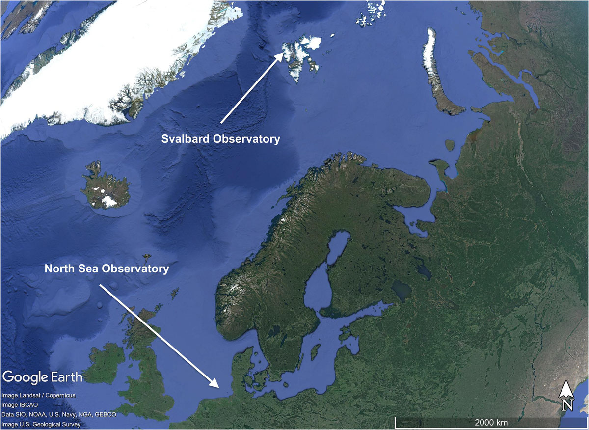
Figure 1. Location of the two COSYNA observatories in the southern North Sea (COSYNA-Helgoland) and the Arctic Ocean in the Svalbard archipelago (COSYNA-AWIPEV).
The COSYNA-AWIPEV observatory is located in the Kongsfjorden Arctic fjord system at 78°55′50.37″ N/11°55′12.10″ E (WGS84), at 10 m water depth (± 0.7 m SD tidal amplitude) on the west coast of Spitsbergen (Fischer et al., 2017; Figure 1). The site is comparatively sheltered in the inner part of the Kongsfjord, with average tidal currents of 0.1 m s–1 (Fischer et al., 2019b). The major threat for any fixed scientific installation in this polar area are freely drifting small and medium sized ice bergs. Until 2006, the fjord was regularly covered by sea ice in winter (Gerland and Renner, 2017). From then on, regular winter ice cover has become rare (Cottier et al., 2007) and closed winter ice cover has no longer been observed since 2009. This is mainly attributed to the increasing warming of the fjord system due to the influence of climate change (Kortsch et al., 2012). This leads to the situation that today, icebergs which are frequently calving from the glaciers inside the fjord are no longer locked by sea-ice but are freely floating in the fjord system reaching the shallow water areas, thus posing a considerable threat to permanently installed measurement systems. With significantly fluctuating minimum winter water temperatures between -1.6 and 0.8°C in February and March, and maximum average water temperatures of more than 6°C in August (Fischer et al., 2018b,c,d,e,f,g,h), there is an on-going discussion as to whether the fjord has exceeded a “tipping point” and will remain permanently ice-free in the future.
A further challenge in terms of continuous operation and regular maintenance of the COSYNA-AWIPEV Underwater Node System is the polar night with a dark phase from November to February and air temperatures below -30°C. This circumstance limits extensive maintenance work under water to the summer months and makes winter operations in the event of system failures a challenge for the participating scientific staff, the scientific divers and the equipment.
Observatory Layout: Configuration Requirements and Implementation
Both node systems have been developed and operated since 2010 as part of the COSYNA framework (Baschek et al., 2017). They were expanded since then as part of the ACROSS and MOSES projects. The main objective was to develop a cabled underwater node system for shallow water areas between water depths of 5 and 300 m. The system was to withstand the challenging environmental conditions in the North Sea and the Arctic with the requirement that it be continuously operated year round and fully controlled remotely. The weight of a single component should not exceed 1 t, so that it could be deployed with smaller coastal vessels using a standard ship crane. A further requirement was that all single components can be mounted or dismounted individually underwater by divers. An additional major requirement was that scientists must be able to operate a sensor at the node system without familiarity with the back-end software technology. Based on these requirements, two industrial (SME) partners were selected to develop a concept for the node hardware and software in a consortium with the participating institutes and to construct a corresponding prototype.
In Figure 2, a sketch of the COSYNA underwater node deployment configuration is shown. The system consists of a land station (1), the submarine cable (2), the actual underwater node (4) and a connected lander system (6), which serves as a basic sensor carrier. The system’s operational range – that is, the maximum cable length for connecting the land station and a first underwater node system – was defined at 10 km. This maximum distance was constrained by the requirements to reach different areas of sediment types around the designated test area of the first node system, the island of Helgoland in the southern North Sea. The concept, however, includes a range extension of up to 30 km by daisy chaining two further node installations.
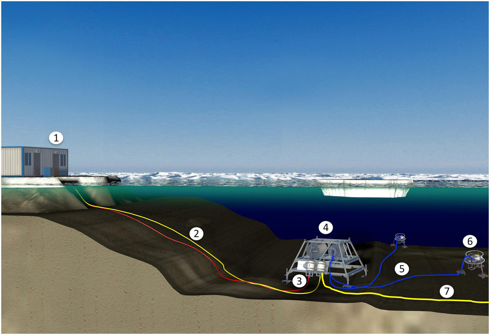
Figure 2. Basic deployment concept of the COSYNA Underwater Node System: (1) land station, (2) submarine cable (1000V), (3) breakout box, (4) underwater node, (5) Power (48V)/TCP-IP hybrid cable, (6) sensor carrier (lander), and (7) submarine cable (1000V) to daisy chained second node. The maximum distance from land station to the first node respectively among the daisy chained second and third nodes is 10 km. Maximum water depth is 300 m. See text for a detailed description of the single components.
The land station (Figure 2(1)) comprises one ARGOS 1200 power supply unit for each node7. Each unit delivers up to 1000 V and 1.2 A, thus providing an input power of up to 1200 W per node to the sea cable. The supply system is based on direct current (DC), which has a lower voltage loss on longer distances compared to alternating current (AC). Depending on the distance from the land station to the node system, the voltage delivered by the land station can be reduced to prevent the transfer of unnecessarily high voltages via the underwater cable and plugs (see also results section “Underwater Pluggable Cables and Connectors”). This is done, for example at the Svalbard node system, where the distance between the land station and the underwater node is only 200 m. There, the input voltage could be reduced to 250 V without any power limitations for the sensor operation.
As IT infrastructure, a VMware ESXi hypervisor, Version 5.5 was hosted one a local server with local storage (Dell PowerEdge R710, 12C, 96 GB RAM, 2,4TB Raid6 Storage). This early setup was replaced in 2016 by a redundant server infrastructure both at the Helgoland and the Arctic node system. It consists of two VMware ESXi hosts, Version 6.5 (Dell Power Edge R730, 8C, 192GB RAM) and two iSCSI storage units with each 5TB Raid6 storage. Full seamless fault tolerance is given this way for the failure of one storage unit or one ESXi host at either site.
The 6-core (6 × 2.5 mm) sea cable (Figures 2(2), 3) is used together with four single-mode fiber optic lines for data transmission. The cable is reinforced with an aramid sheath and has a copper foil shield with a double wire. The coating is made of polyurethane and the outer diameter is 22 mm. The cable is approved for an operating voltage of 1000 V DC, with a test voltage of 4 kV AC. The cable resistance is 3.3 Ohm/km; the weight is 705 kg km–1; and the maximum tension load is 2000 N. The calculated voltage drop is 6.9 V km–1 at 1000 V and 1200 W (maximum power transmission). This results in a maximum power drop of up to 207 V at a maximum distance of 30 km from the third node to the land station in the full expansion stage with daisy-chained node systems. For data connectivity, one pair of the fiber optic lines is used to establish a 1000-FX network link to the land station. A further capacity extension by upgrading the fiber optic transceivers is possible.
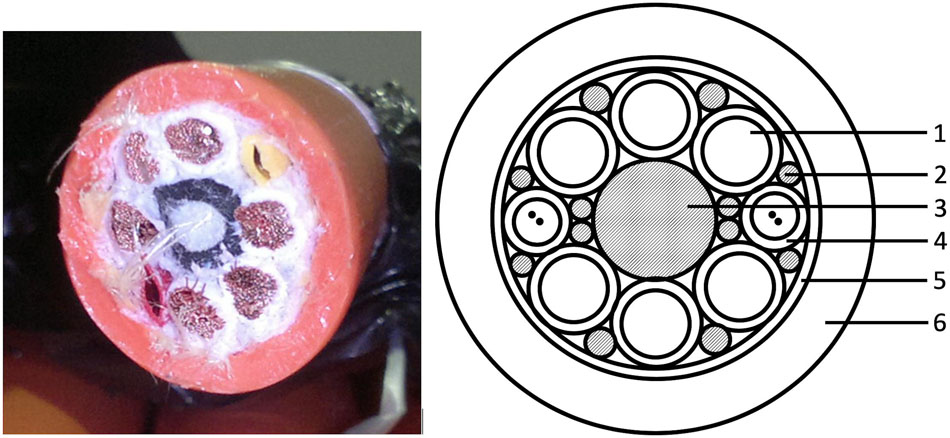
Figure 3. Sea cable (diameter 22 mm) used to connect the land station with the node system (1 = insulated cores, 6.0 mm2; 2 = filler; 3 = GRP fabric; 4 = fiberglass cable single mode; 5 = taping; 6 = outer sheath. For additional details see text). Photo: P. Fischer.
The submarine cable is connected to the underwater node system at the “breakout box” (Figure 4). In this cable termination, the optical fiber connection of the underwater cable is converted into a copper-based data transmission. The incoming 1000 V are converted to 48 V to supply the electronic components in the breakout box. This large-step power conversion was achieved by a special power supply unit from SYKO Type BLG.M. The IT components used are active components with their own IP addresses to communicate with the components and check their function in the event that either no node is connected or an undefined error occurs in the system. The breakout box is constructed of polyethylene (PE) and is approximately weight-neutral in water. An IP-based water intrusion detector is mounted to monitor it.
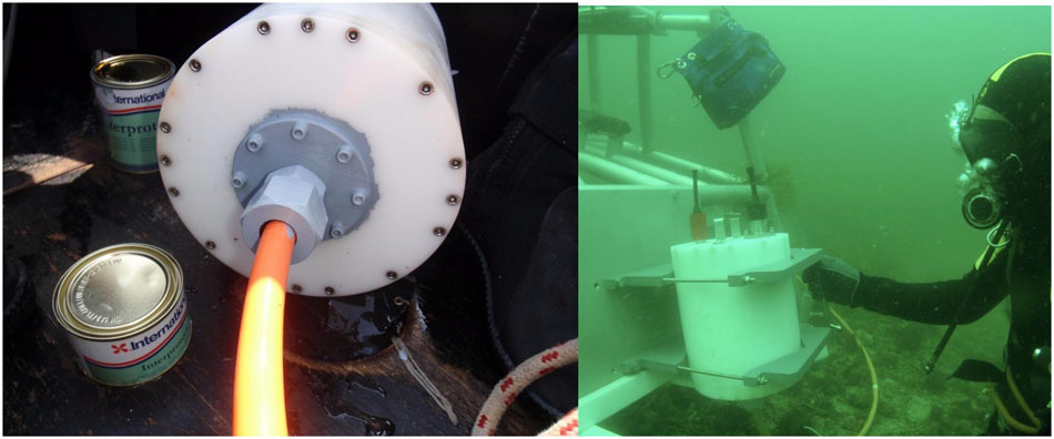
Figure 4. Left: Sea cable feedthrough coated with corrosion protection. Right: Breakout box mounted on the frame of the Helgoland underwater node system. Photos: P. Fischer.
Figure 5 shows the complete COSYNA Underwater Node System during operation. The breakout box is connected to the node by two wet-mateable cable connectors: one connecting the power (1000 V – type DC), and the other connecting Ethernet (1000BASE-T).
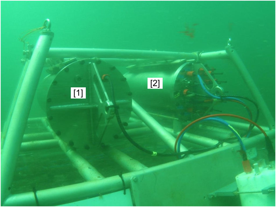
Figure 5. Fully operational node system off Helgoland. The left tube (1) houses a battery pack that provides power for 2–6 h, depending on the power consumption of the sensors. The right tube (2) is the node system which is connected to the breakout box by the red 1000 V power line and the blue Ethernet line. On the front panel, ten sensor ports are available, each providing up to 200 W and an Ethernet connection. All cables between the different node components are wet-mateable by divers, except for the sea cable that enters the breakout box from below via a permanent cable feedthrough (see Figure 4). Photo: P. Fischer.
Communication and data transfer from and to the underwater node systems is performed by standard internet protocol TCP/IP. From 2012 to 2015 at the Helgoland systems and until 2016 at the Svalbard system, the land stations of the nodes were connected via IP radio relays over a distance of up to 60 km to the respective national IP network. Even though these connections were sometimes identified as possible bottlenecks for remote node operation, especially in the Arctic, they never restricted the required bandwidth. From 2015 onward at Helgoland (Germany) and from 2016 onward at Svalbard, a cable-based fiber optic connection via the respective national sea cable infrastructure is available for data transfer.
The internal power of the underwater node system and connected sensors is set to 48 V to allow for safe underwater operation by divers when the 1000 V land power supply must be shut down. To keep the system running during intentional (or unintentional) power cuts, an additional battery buffer is installed (Figure 5(1)), keeping the system alive for at least 2 h so that divers can safely approach the system under fully operational conditions.
For attaching sensors (or even complex sensor units) to the node, ten underwater mateable connectors are available per underwater node, each providing 100BASE-T ethernet link (max. 1000BASE-T ethernet) for data transfer, and a 48 VDC power supply with a maximum of 200 W per connector (Figure 6, right image). IP-based Ethernet connections are used as standard transport protocol. Non-Ethernet sensors can be connected via specific “connector boxes” containing hardware to adapt sensors to serial or USB interfaces (Figure 6). The connector boxes have been specially designed and developed for the COSYNA node system. They can be individually configured depending on the sensors to be connected. The boxes are made of POM material (polyoxymethylene) which is commonly used in marine engineering and they are standardized in size. The standard connector box has a diameter of 27 cm and a length of 38 cm and can be equipped with various underwater pluggable connectors in the lid. Connector boxes only differ in the length of the body and not in the lid, so that the lid with the connectors and the wiring can be used with a larger body if additional space is needed. A COSYNA standard “connector box” can take up to six sensors and provides 12, 24, and 48 V as well as standard RS232 and RS485 communication at each of the six ports. For other sensors, a custom configured “connector box” is provided based on the standard input of 48 V and a 100 Mbit Ethernet connection from the node. For all sensor communication via the node to the user, industrial Ethernet-serial/USB converters (AdvantechTM EKI 1524 or WUTTM Com-Server Serial/USB) are used.
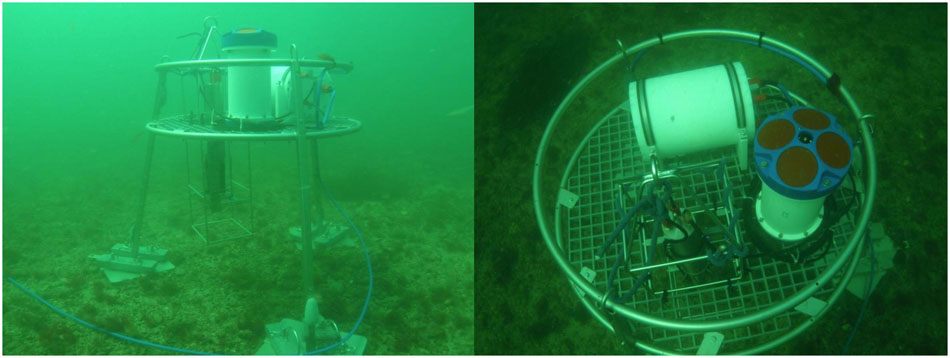
Figure 6. Sensor lander with a “connector box” (white PE tube in the right image). The “connector box” is connected to the “breakout box.” From there, a serial, USB or any other sensor is connected via the respective communication protocol. The respective Ethernet interface for a sensor is installed in the “breakout box” and connected to the sensor via an underwater mateable subcon plug. The photographs show a COSYNA “standard lander” that is equipped with a Sea&Sun CTD, a Teledyne ADCP and a SeaBird SBE38 temperature sensor. The standard “breakout box” can take up to six sensors and provides 12, 24, and 48 V as well as standard RS232 and RS485 communication at each of the six ports. For other sensors, a custom configured “breakout box” is provided based on the standard input of 48 V and a 100 Mbit Ethernet connection from the node. Photos: P. Fischer.
Standard Data Provided by the COSYNA Underwater Node System
Each COSYNA Underwater Node System is connected to a standard lander (Figure 6, left) carrying a sensor package that measures basic oceanographic parameters (Baschek et al., 2017) continuously year round. It comprises an upward looking ADCP (Teledyne Workhorse 1200 kHz), sensors for pressure, temperature, conductivity, oxygen, chlorophyll-a fluorescence, and turbidity integrated in an extended CTD (Sea&Sun CTD90) and temperature logger (SBE38). All standard oceanographic parameters are publicly available in near realtime (based on the logger after 1 or 24 h) on the COSYNA data portal8 and the AWI web page9. Both data portals offer CSV formatted data for download. The COSYNA data portal offers additional SensorML format via the web service OGC-SOS, the AWI dataportal offers JSON format. Discussions in the scientific community revealed, that most biological oceanographers prefer the CSV format, more standard oriented scientists prefer SensorML or netCDF and data scientists often prefer JSON. Even though the three latter data formats are more efficient with respect to information per data volume, according to our experience it is highly recommended to at least provide one “low-level” data format for download to make data accessible in the context of FAIR also for non-data specialists. On the other hand, CSV formatted data do not fulfill the FAIR criterium of interoperability because CSV files are not per se machine readable and linkable. It will certainly require further efforts to implement the FAIR standards for all user groups. An important step in this direction would be the consistent implementation of simple to use import routines for FAIR data formats in the most common spreadsheet programs and the provision of easy-to-use import routines for FAIR data formats in the common script languages such as R or Matlab.
User Operation of the COSYNA Underwater Node System
The COSYNA system is designed to enable sensor owners to operate their sensors at the underwater node without special knowledge of specific electronics and IT. Nevertheless, the sensor owner must provide basic information about the sensor itself (i.e., the sensor’s user manual), about the power requirements of the sensor (voltage and current consumption) and the type of digital communication. The comparatively strict procedure of answering a questionnaire in advance proved to be necessary in the course of integrating the first sensors to avoid misunderstandings between sensor owner and node operator and to avoid malfunctions, or even damage, to the sensor during integration. Based on this information, the physical integration of the sensor is prepared in the lab. There, the user must demonstrate that the sensor will function properly on a computer for at least 24 h with the defined power supply and that the software used for data acquisition (e.g., the original software from the sensor manufacturer) will demonstrate working stability. The final implementation of the sensors in the node system, including the mechanical, electrical and IT integration of the sensor as well as setting up and managing the user access to the sensor, is managed by the COSYNA node consortium, in which the two participating partners – Helmholtz-Zentrum Geesthacht and Alfred Wegener Institute Helmholtz Centre for Polar and Marine Research – are represented.
New sensor integration into the Arctic underwater node system is more extensive than for the North Sea node, as there, sensors are only accessible once or twice a year. In order to ensure the operational stability of these sensors, an integration and in situ test operation phase of at least 14 days at the North Sea node has proven to be important to ensure the reliability of the software and hardware components as well as to ensure the capability of complete remote control in terms of power and network. Since the North Sea and Arctic node systems are more or less identical in terms of hardware and network configuration, it is thus ensured that a sensor successfully operated at the North Sea node will also work at the Svalbard node system.
The final access to a sensor or to multiple sensors mounted at either node is established with virtual computers that are set up on the central server. A virtual machine is a software-based individual workstation on which different operating systems (Windows, Linux, Unix) can be installed. Access to the virtual machine is provided through remote login via an open source or a commercial remote login program, whereby the programs “Real-VNC”10 and “TeamViewer”11 have become the most popular in the COSYNA consortium. The user has full user rights to install software on his or her workstation to operate a sensor, and each workstation has a standard hard disk size of 500 GB to temporarily store sensor data. This system architecture allows the user to operate a sensor from anywhere in an identical manner and with the same software as used directly in the laboratory without the underwater node system infrastructure.
Data acquisition is important with respect to the software required for continuous sensor operation. For many sensors, only interactive sensor control software is available that requires manual interaction to store data files, read calibration data, or perform other operations. The development of software that allows fully automated operation of sensors, including data storage, is usually costly and requires special programming for each sensor type. Within the framework of the node system development, we developed an alternative way to operate sensors permanently and resiliently without an additional probe-specific software solution. For this purpose, the software “MacroScheduler” was used to code every action a user performs on the screen with a keyboard or mouse into a stable executable program. With this procedure, it has been possible to fully automate any original sensor software thus far. This has the additional advantage that the generated data files can be read with the original software and, if necessary, processed further.
In parallel to the optimization and development of the node hardware, the importance of timely, resilient and, in particular, traceable plausibility and quality checks of the measured data emerged in the course of the operational phase. Especially in case of cabled observatories, the tendency and the willingness is great to feed the measured data directly into respective databases and thus to make them immediately available to science and to public stakeholders, especially when the financial support of the systems may depend on this “real-time” data availability. Without reliable and widely automated quality control procedures, there is a considerable risk that unreliable or, in the worst case, false data, e.g., due to sensor failures or sensor drift, may become available and be used by the scientific community or the public. Furthermore, initiatives such as “FAIR” (Wilkinson et al., 2016) address the importance of adequate metadata for each sensor without which it is often not possible to use the data for scientific analyses. In the COSYNA framework, this requirement has been taken into account by checking all oceanographic basic data (see section “Standard Data Provided by the COSYNA Underwater Node System”) according to the international standard (SeaDataNet, 2010; Breitbach et al., 2016) prior to their transfer to the corresponding data portals. This ensured that at least impossible or improbable data were clearly marked as “bad” data and therefore could be excluded. In the course of the continuous operation of the two systems, however, it became clear that pure and fully automated plausibility checks, even though internationally accepted, were not sufficient to provide “good” data. We therefore developed a multi-step machine-human procedure to convert probably good data (data which passed the automated flagging routines) into “good” data. The procedure is entirely written in R and uses well published procedures for data de-spiking, data imputation, data cross-validation and visual data inspection and will be published separately. Even though it will never be possible to 100% avoid wrong data in datasets especially from continuous operating observatories, such multi-step machine-human procedure significantly help to minimize the risk of distributing erroneous scientific data and should therefore be always made available together with the respective datasets.
Results
Similar to moorings or other autonomous sensors, cabled underwater observatories offer the opportunity for temporal high-resolution long-term measurements in areas where it is difficult to perform manual sampling all year round. In addition, automated sensors can form the backbone of intensive measurement campaigns so that discrete sampling, for example, with (costly) research vessels can concentrate on collecting non-automatically measurable variables. In addition to moorings and autonomous sensors, cabled observatories also allow the use of highly complex sensors that need frequent human interaction for reliable operation – even in remote areas where access is limited. At both underwater observatories, in Helgoland and in the Arctic Kongsfjorden fjord system, we successfully operate additional complex stereo-optic sensors and a video-plankton recorder to assess the local fish, macroinvertebrate and plankton community in detail. These sensors provide large datasets of high-resolution images of a certain water volume or benthic area. The images are transferred online directly to Germany, where they are analyzed for total species abundance, species composition, and species-specific length-frequency distributions (Fischer et al., 2007; Wehkamp and Fischer, 2014).
Even though optical systems can be deployed also autonomously, cable connected systems have the advantage of more or less unlimited power supply and storage volume for the images. Furthermore, image analysis is often time consuming especially when no fully automated object detection and measurement algorithms are available, a field of data science in aquatic ecology which is just emerging (Marini et al., 2018). Images are delivered in near-realtime every day and can be analyzed continuously which is often more feasible than analyzing thousands of images after an instrument has been recovered. In addition, 100% autonomous operation over longer time periods is not feasible for such installations. The likelihood is high that such complex systems fail at some point and therefore need human interaction for proper operation. Such systems, however, can nevertheless be operated steadily over long periods of time at cabled observatories because they can be continuously monitored with automated routines, and many failures and problems during the operation can be fixed remotely. Furthermore, the samples (e.g., images, videos, acoustic recordings) can be transferred or streamed online to any land-based server, where the samples can be processed and analyzed in real or near-realtime so that not only the functionality of the sensor itself is controlled but also the scientific analysis can be done continuously and concomitantly with the sampling process itself. The latter point in particular is advantageous allowing a rather interactive than static sampling scheme where field campaigns can respond rapidly to signals from the environment, such as the start of the spring bloom or the occurrence of certain species in an area. This is especially advantageous for remote field activities and can make the often costly and labor intensive in situ sampling more targeted and efficient.
Figures 7, 8 show two examples of such labor-intensive samplings that are impossible to perform without cabled observatory technology. Figure 7 (left panel) shows a year-round assessment of the fish and macroinvertebrate community in Svalbard’s Kongsfjord in the years 2013 to 2014 using the RemOs1 3D imaging sensors (Fischer et al., 2007).
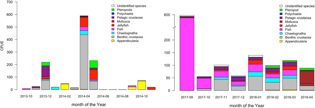
Figure 7. Data from the RemOs1 stereoscopic fish observatory attached to the underwater node system in Kongsfjorden. Left panel: Year round survey from October 2013 to November 2014 (modified after, Fischer et al., 2017). CPUE (catch per unit effort) is an arbitrary unit showing the total mean number of specimen counted per week based on 48 stereoscopic image pairs (one image pair every 30 min) summed up per week. Right panel: The same analysis performed for the period September 2017 to April 2018.
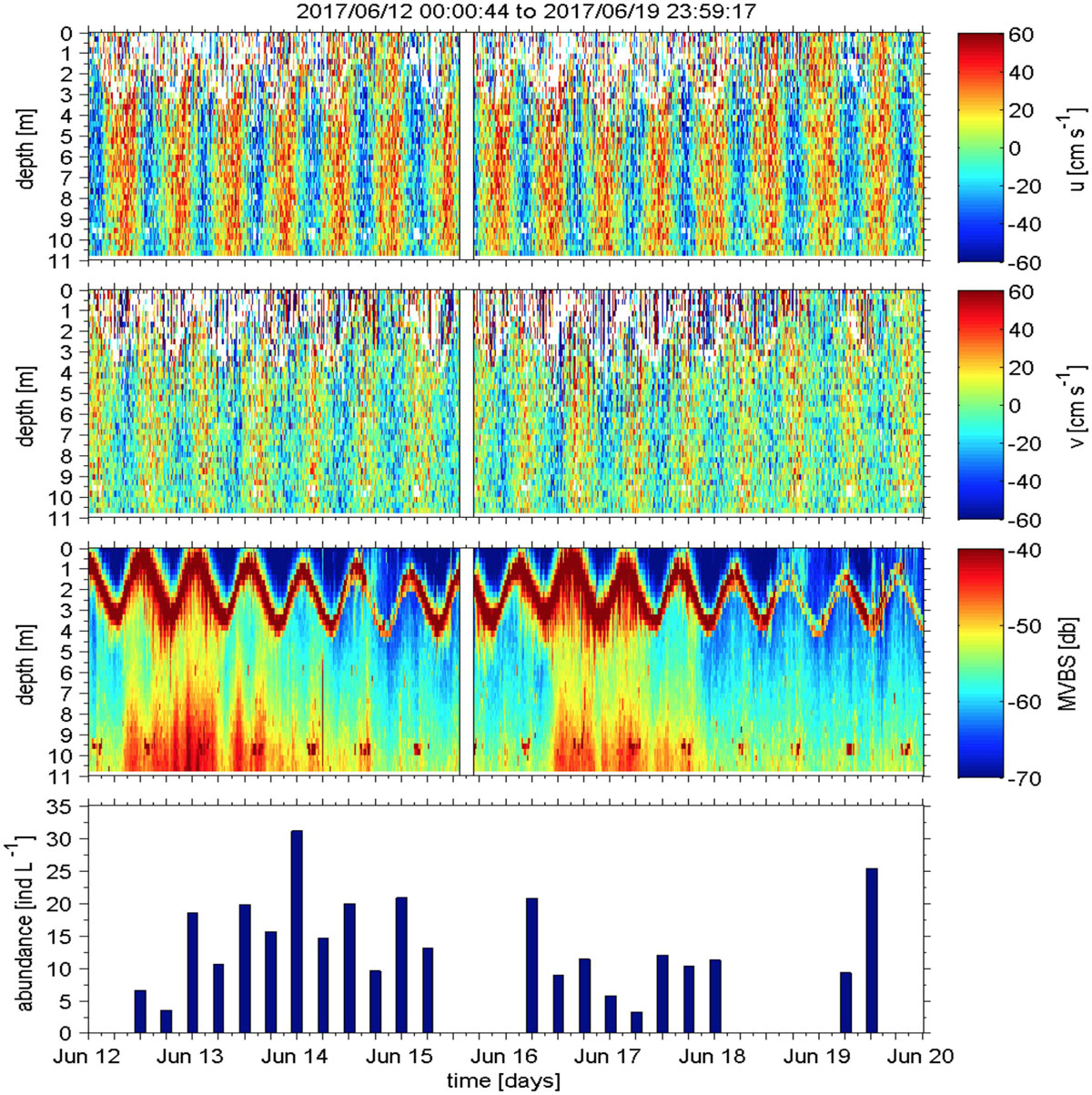
Figure 8. An 8-day sample (2017/06/12 00:00 to 2017/06/20 00:00) of horizontal velocity components u and v as well as backscatter estimated from the ADCP, moored about 500 m north of the island of Helgoland at a depth of around 10 m at the AWI underwater experimental field “Margate.” The lowermost panel shows the total abundance of plankton and particles derived from the VPR measurements (no data = underwater maintenance work at the observatory).
The profiling optical sensor takes high resolution stereoscopic images with a frequency of one image pair every 30 min and is positioned every week in five different water depths for at least 24 h. Moving the system vertically was done by an in-house designed remote-controlled winch system in combination with a depth sensor (Figure 9D) allowing to vertically position the entire system in any depth between the surface and the sea floor. The water column in the littoral zone is thus completely assessed once a week, with 2 days to spare for repeating depth strata that were missed – for example, due to technical problems or poor visibility. The system facilitates measurements of species abundance, species composition and species-specific length frequencies, while providing unique time series over the 24 h diel cycle continuously for 365 days of the year. The observatory enables repeated sampling every year as shown in Figure 7 (right panel) for the season 2017–2018. This long-term sampling provided the world’s first year-round dataset of the littoral fish community in an Arctic fjord system and confirmed the hypothesis that the polar night is rather important for the fish and macroinvertebrate community in very shallow areas. The development and operation of the COSYNA Underwater Node System enabled year-round collection of oceanographic variables together with quantitative data of higher trophic levels in an extremely hostile environment with air temperatures below -30°C and complete darkness during some times of the year. This made completely new insights into the temporal dynamics of this polar shallow water ecosystem possible (for details see Fischer et al. (2017).
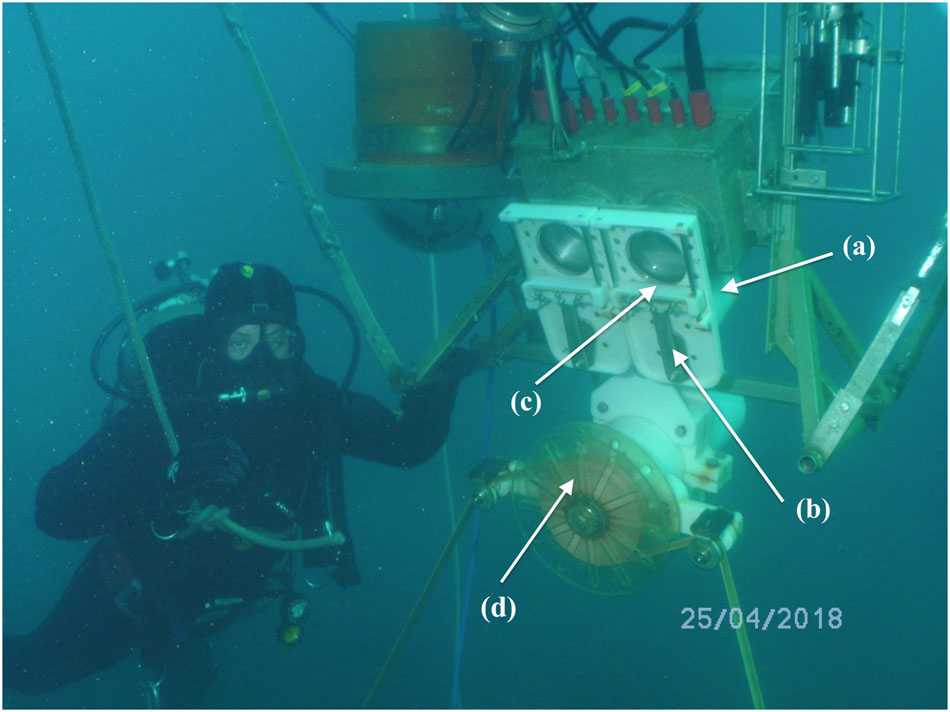
Figure 9. Stereo-optical unit in Kongsfjorden with a mechanical cleaning system (see arrow) for the camera lenses. For each lens, the system comprises (a) a remotely controlled electrical power unit, (b) a connection rod transferring the rotation of the engine to a vertical movement, (c) a wiper construction moving up and down to clean the lens systems, and (d) remote controlled winch system for vertical profiling and positioning the system in the water column. Photos: P. Fischer.
Figure 10 shows a sketch of the remote controlled zooplankton observatory attached to the Helgoland underwater node since 2016. This device is based on the combination of an Acoustic Doppler Current Profiler (ADCP RDI Workhorse Sentinel 1200 kHz, Teledyne RD Instruments USA, Poway, CA, United States) with an underwater imaging system (Video Plankton Recorder, VPR Seascan Inc., United States). The ADCP provides a three-dimensional measurement of the flow field and measures the acoustic backscatter strength, providing continuous high resolution data, for example, to yield precise estimates of timing, velocity and extent of the diel vertical migration of zooplankton communities (Cisewski and Strass, 2016 and Figure 8).
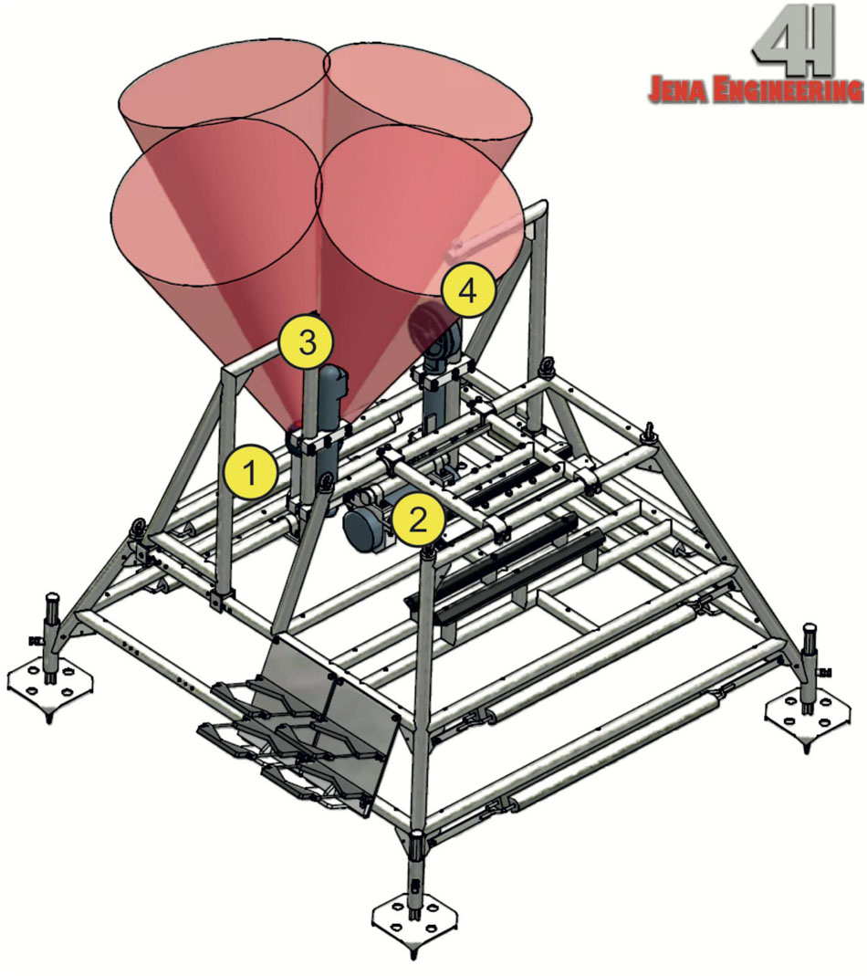
Figure 10. Sketch of the Zooplankton Observatory consisting of (1) a Workhorse Sentinel ADCP (1200 kHz), (2) VPR electronics housing assembly, (3) camera housing assembly and (4) strobe light housing assembly.
The VPR records high-resolution digital images with a frame rate of 15 s–1, illuminated by a ring light strobe synchronized with the camera shutter. Four calibrated magnification levels allow the focused imaging of plankton and particles within a size range of 50 μm to several millimeters and thus enable a quantitative optical sampling and size estimate of marine aggregates and fragile species. This includes gelatinous plankton, which is often undetected or underrepresented in the traditional plankton sampling methods (Möller et al., 2012). Both instruments are mounted on the COSYNA node rack in a manner such that one beam of the ADCP (depth cell size 25 cm, sampling interval adjusted to one ping per ensemble with a ping rate of 1 min–1) intersects the focal depth of the camera (Figure 10) to cover the same volume of water. Plankton and other particle images are automatically extracted from each image frame as regions of interest (ROIs) using the Autodeck image analysis software (Seascan Inc., United States), saved to the computer hard drive as TIFF files and immediately tagged using the system’s timestamp. This allows later merging with the ADCP and hydrographic parameters.
All images are sent to the land-based server for further processing, where they are classified automatically into taxonomic categories following a method by Hu and Davis (2006). The average power consumption of the entire system including node, sensors and VPR is about 120 W in standard operation mode and the volume of image files from the VPR is app. 20 GB h–1. This and the required intermittent human intervention, reprogramming of the system clearly demonstrate that such high-end optical systems cannot reasonably be operated autonomously year-round without cabled observatory technology.
The Node Hardware
Experience has shown that almost all generic and sensor-specific developments or experimental designs required significantly more time in operation than industrially tested software and hardware. Nevertheless, for some experimental approaches, no off-the-shelf components are available, so that in-house developments are necessary. However, this decision should be carefully examined on a case-by-case basis, as industrial solutions sometimes do exist, which are, however, more expensive initially. For off-the-shelf solutions, however, the financial expenditure is shifted from the investment to the operating expenses. It is important to consider that repairs or adjustments during operation are always associated with the risk of data failure or loss.
In addition to several small changes and optimizations that have occurred over the years during the operation of the nodes, three major problem areas have emerged, each of which has had a lasting effect on the operation of the underwater node during certain phases. These three problem areas were the underwater plug connections, the (non-)availability of essential housekeeping data for error analysis of the system in case of malfunctions as well as the basic software architecture for sensor data processing.
Underwater Pluggable Cables and Connectors
One of the main features of the COSYNA underwater node is that all individual components – the node, the external battery pack and the sensors – can be exchanged underwater by scientific divers without having to recover the entire system itself. The individual components are therefore connected by cable connections that can be plugged in under water. During the design and construction of the system, special care was therefore taken to ensure that all connectors used were certified by the manufacturer for underwater connection.
During operation, however, it was found that this specification was not fulfilled. Problems arose, in particular, at the main power connection, which delivered up to 980 V to the node. These plugs were officially certified to 1000 V, but failed after only 3 months with a short circuit, although the manufacturer’s handling instructions were followed precisely. This stipulated that both the plugs and the sockets, if they are to be plugged in under water, must be treated with a thin layer of a special grease supplied by the manufacturer. The analysis of the damage showed that the (+) pins of the 1000 V plug were completely burnt and the jacket of the plug had melted (Figure 11), so that sea water had penetrated the plug and led to a massive short circuit on the socket end as well.
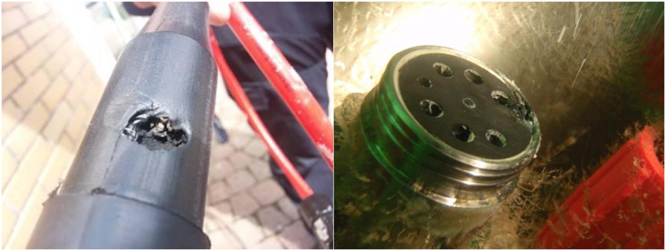
Figure 11. Underwater plug and respective socket of the 1000 V power input circuit after severe damage. Photos: P. Fischer.
The manufacturer informed us that this damage could only be the result of improper handling. We modified the manufacturer’s handling instructions and filled all sockets under water completely with a syringe filled with the grease recommended by the manufacturer. This alteration extended the operating time of the connectors to almost 9 months. After that period, however, there was another short circuit and the plug and socket were completely destroyed again.
Based on these events, the company commissioned its own investigations into the plugs. They found that the resistance between the individual plug pins was much lower when they were plugged in under water than when they were plugged in on land, regardless of whether they were properly greased or not. The company offered to replace all underwater plugs and cables, worth approximately €45,000. In addition, the manufacturer’s instructions for greasing the plugs was updated, the manufacturing process of the plugs themselves was modified and the manufacturers recommendation for the type of grease to be used for underwater mating was changed to a 100% carbon-free product.
Logging of Housekeeping Data
A second major issue in the operation of the nodes turned out to be incomplete housekeeping data. In the first node version, the input power on land and the output power at the sensor ports were available as housekeeping data and as Boolean information regarding the leak tightness of the underwater housings and the operating temperature of the individual components.
Continuous and largely unattended operation of the system showed that additional housekeeping data is required, particularly in the event of system malfunctions and failures. It turned out during operation that the originally selected variables and their recording frequency were insufficient.
As already mentioned, the most critical components during operation were not the electronic components in the node, but the cable-bound connection between the individual components. The first node generation did not include an explicit infrastructure for a continuous and higher-frequency logging of the undisturbed functionality of cables between the node components. As a result, it was often unclear which component of the system was affected, resulting in unnecessary recovery of all node components or lengthy underwater troubleshooting and testing. Based on this experience, we decided to equip all pluggable cable connections with appropriate sensors for voltage on both ends in order to obtain detailed information on where a possible malfunction is located. The availability of this information significantly accelerates troubleshooting, as defects in cables and connectors can either be detected so early in operation that a problem can be prevented, or malfunctions can be found and corrected more quickly (in case of internal system component failures. In this context, we experienced that in addition to the continuous monitoring of the voltage and current parameters, a continuous monitoring of the residual currents of the power lines is of critical importance. Residual current measurements provide information about the insulation condition of the cables and connectors against the surrounding water. Particularly in the case of the underwater mateable connectors, a slow increase in the residual current indicates a gradual loss of insulation of the connector, e.g., due to the washing out of the insulation grease. This problem can then be solved in time and without potential damage by re-greasing the plug connections under water.
Node Control Software
The overall power management of the underwater node (switching the individual ports on and off and providing power to the sensor ports) as well as the node monitoring (power consumption and network activity) is realized by Programmable Logic Controllers (PLC) with discrete software. The first prototype node used Siemens Simatic S7 PLC, which was replaced in rebuild by a Beckhoff CX8090 CPU. Both PLC solution were equipped with required analog and digital I/O modules. The remote control and monitoring is realized via a web frontend and IP, and all available information are logged in a SQL database for system monitoring. This frontend has three access levels: “user,” “port administrator” and “system administrator.” As of now, “users” are allowed to see the status of all ports (i.e., see if a specific port is on or off); “port administrators” are allowed to switch all ports on and off and to change the maximal power (watt) that the individual ports deliver; and “system administrators” have full access to the system, including adding new users with password settings.
This software design proved not to be ideal for an infrastructure used by several independent groups in parallel. In particular, the roles and privileges of the “user” and the “port administrator” were not well designed. Currently, “users” only have read/write access to a port for accessing a sensor and downloading data. In order to switch off a sensor completely, “port administrator” rights are required. “Port administrators,” however, cannot be enabled for single ports only, but have access to all ports and extended functions of the node. This leads to the consequence that external users are only assigned the role of “user” and thus cannot switch their own sensor on and off. This is especially problematic with sensors that are not completely developed or automated either in terms of the hardware or the software and therefore frequently must be disconnected from the power supply network in order to reset.
Software Issues With Respect to Sensor Operation
In the very beginning of node operation, two different scenarios of sensor operation were planned: (a) the operation of sensors for standard parameters by the node consortium itself and (b) the operation of sensors from external partners under the full responsibility of the external users. The external users, in particular, were thought to be fully responsible for their data and, after the initial installation phase, also for the remote sensor operation and monitoring. Both scenarios were adapted based on the experiences of the first year of node operation. Scenario A was initially designed as a type of real-time operation, where the sensor data were to be streamed directly to a central database at the Helmholtz-Zentrum Geesthacht. While the basic principle of this real-time streaming approach works well for our set-up and is still in place, some shortcomings of a pure streaming procedure became apparent. Many sensors do not deliver “to go” data directly from the sensor itself but “raw data,” such as voltage, a digital or a binary output. This data must be processed by software using calibration coefficients or conversion algorithms to obtain the target parameters in the correct units. With direct streaming, the raw data (e.g., Volt) are converted by generic software “on the fly” into scientific values which are then directly fed into the database, however without storing the original raw (e.g., Volt) data. This holds a considerable risk in case the calibration files are technically decoupled from the probe and can thus be unintentionally confounded. In 2014, this “on the fly” conversion resulted in almost 2 month data loss from a specific sensor, because the wrong calibration file was used. Because the raw data (Volt) were not stored, the scientific data could not be recalculated with the correct calibration file. To prevent this, it was decided not only to stream the final scientific readings from each probe, but also to store the raw data from each sensor in the highest possible temporal resolution (e.g., in volts at 1 Hz) every hour in single files. This makes it possible, in case of accidental use of the wrong calibration file, to recalculate the data completely afterward. Additionally, it was decided to implement additional security procedures for the data transfer to the respective databases to avoid the transmission of erroneous data in the data portals and to ensure that there is no missing metadata for individual sensors. From 2016 on, the transfer of data into the database itself was obligatorily linked to the availability of a minimum of up-to-date metadata which means that if metadata were missing, no data entry would be possible at all. This strategic upgrade of redundant data acquisition and storage procedure proved to be extremely reliable and allows post-processing of all data in case of a failure in the real-time streaming process occur.
To store raw or scientific data in discrete hourly files, we prefer to run the original program provided with the sensor. This has the advantage that the program can undertake all raw data conversions and usually delivers “readable” ASCII files, which can be used for further processing with standard programs. Only very few sensors come with programs that would enable the sensor to run fully automatically for several months and save data files at pre-defined time intervals. We therefore use the macro scripting language “Macro Scheduler” to make these non-scriptable programs fully automatic and remotely controllable. This is done by simulating user interactions in macros, which then can be run in pre-defined time intervals, such as every 60 min or 24 h. This procedure proved to be extremely efficient and reliable, especially when integrating new sensors into the network.
The second sensor operation scenario (sensors operated by external partners under their own full responsibility) more or less failed. Our expectation was that most external groups that asked for the opportunity to operate a sensor at the underwater node were experienced in remote sensor operation and that it would be sufficient for us to provide assistance during sensor integration. This assumption turned out to be unrealistic. Most users approaching us to operate a sensor, either in the North Sea or in the Arctic, are experienced in manual sensor operation and data handling but not in remote controlled automated sensor operation. To remedy this finding, we also applied our internal sensor operation procedures to the external partners. We offered not only to install but also to operate the sensors, utilizing our automation and data saving routines, and most often also using automated data file delivery to any server or e-mail address. It turned out that this “full service” was a better solution for all internal and external partners, often leading to scientific cooperation projects rather than mere infrastructure used by the external partners.
Although the software on sensor control, data transfer and regular node operation developed since 2012 is not so far available in a public repository like GitHub, all scripts and routines are freely available upon request. This is especially true for the complex routines and scripts for data plausibility and quality control, which are mainly written in the script language R (R Core Team, 2017).
Discussion
Underwater node systems are one of the future technologies that can contribute to real progress in coastal ecological research once their technological development is sufficiently advanced. The possibility of a continuous interactive “presence” in environmentally (e.g., weather-related or geographically) difficult focus regions, such as the polar regions or the North Sea, makes this technology highly valuable for answering Earth system questions (Trowbridge et al., 2019). Cabled underwater observatories should be integrated into larger, networks since the digital connection of the sensors to the Internet is readily possible. The two COSYNA node systems presented here are part of the emerging German Digital Marine Network “MareHub” and the German National Research Data Infrastructure (NFDI) as well as part of the European Jerico 3 network. In addition, COSYNA data are delivered to the European Marine Observation and Data Network (EMODnet) and Copernicus Marine Environment Monitoring Service (CMEMS). However, experiences with operating the node systems described here also show that there are still several technical, conceptual and structural problems that must be overcome in order to improve the use of underwater nodes as a fully operational and stable technology for aquatic research in the future. The most important points concern the power supply, the stability of sensors in continuous operation mode and the handling of large data sets by the scientists themselves – that is, the need for user training.
Power Related Issues
During the operation of the COSYNA underwater node system from 2012 to 2018, several power related issues emerged, which intermittently hampered the operation of the nodes and the attached sensors considerably. Table 1 shows a summary of the major power failures during the continuous operation of our observatories. The first two columns compile the sources of failures in the power supply system. Some of the problems listed in Table 1 occurred only once and could be fixed permanently. The central problem that could not be solved by a single repair and is still virulently occurring in our systems is the issue with the underwater pluggable connections. Although the manufacturer has made some modifications to the installed connector types in response to our damage reports (see section “The Node Hardware”), it must be stated that the connector types used are still only conditionally suitable for long-term use under water and must be maintained at least every 6 months. Even though this can be done under water by scientific divers after some training, the problem is not ultimately resolved, and there is a certain risk that the plugs will show malfunctions even though they are properly maintained. During maintenance, particular care must be taken to clean and degrease the plugs and sockets thoroughly and to fill the socket holes again with 100% carbon-free grease (e.g., Parker SuperOLube). When assembling the plugs under water, it is absolutely crucial that the grease is pressed out of the socket holes during the plugging process and that the grease completely fills the gap between plug and socket. This is necessary to prevent seawater penetrating this gap to avoid, for example, small mussel larvae – which are only few μm in size – from settling in this space, growing there and slowly pushing the plug out of the socket.
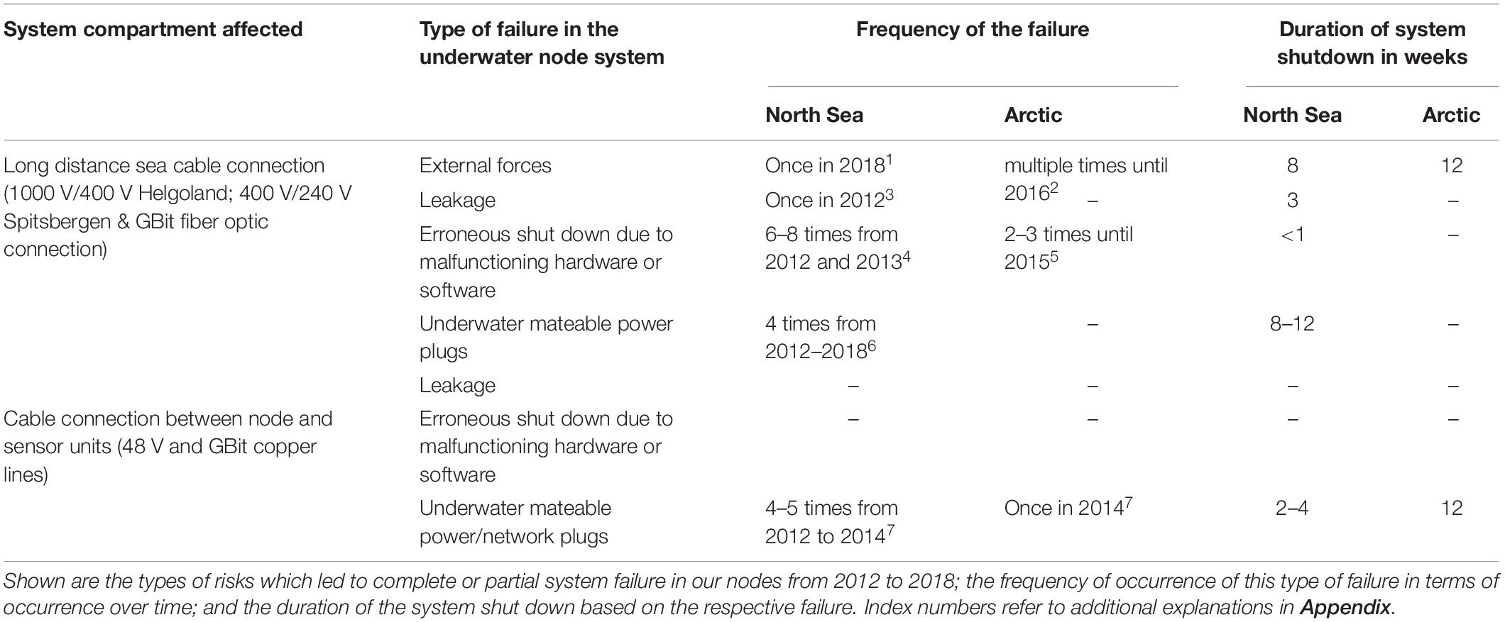
Table 1. Summary of failures of the underwater nodes in the southern North Sea and in the Arctic.
If the procedure described above is followed exactly, it is possible to use medium-priced underwater connectors for shallow water observatories, but with a latent risk of failure. Therefore, to avoid the risk of system failure, industrial plug connections such as GISMA, which are significantly more expensive, however, should be used, especially for voltages above 48 V.
Sensor Exposure Time
A particular challenge for the longer term operation of underwater nodes is the fact that sensors may not be designed for longer term exposure, i.e., for several months. There are only few sensor systems available which have a manufacturer designed device to prevent biofouling and therefore must be cleaned by hand at regular intervals. Furthermore, probe manufacturers typically do not provide reliable information about the temporal drift behavior of their probes or the recommended maximum duration of a measurement until recalibration is required. Some manufacturers do not even provide accuracy and precision values for their sensors, even if they are properly calibrated. This missing information on data quality of sensors lead to the highly unsatisfactory situation that scientists sometimes have to trust sensor data without being able to estimate data accuracy and without a proper knowledge of the probe’s behavior especially during longer time exposure. Because we cannot assume that sensor data, even when a sensor is quite expensive, are correct per se, we need a better implementation of validated data quality control routines in aquatic ecological disciplines. Such procedures are already available (see e.g., Ocean Best Practices System Repository)12 but should be applied as default, e.g., as ready-to-use packages in common software and scripting languages. Until now, automatically generated data are too often not continuously checked for quality from the start and corrected if necessary, but only after several weeks or even months. If no reliable and fully automated control routines are implemented in such a system, errors in the measurements often remain undiscovered for too long and cannot be corrected afterwards. The result is that the data sets must ultimately be discarded.
Biofouling
The problem of biofouling is probe and even parameter specific. While temperature and conductivity sensors are less affected, optically or chemically based sensors face the problem of significant accuracy loss as well as potential precision loss after only a short time, especially in warmer temperatures. While our Arctic sensors were normally perfectly stable for months during the Arctic winter when no light was available, in spring and summer, these sensors were overgrown with periphyton within days or weeks. In the Arctic system especially, when daylight returns in spring, periphyton can grow so fast that “soft” anti-biofouling measures such as UV-radiation (MacKenzie et al., 2019) or gentle acid applications on surfaces cannot cope with the growth rates of the biota. In our case, only mechanical hardware cleaning systems such as wipers were effective in preventing sensor overgrowth and uncorrectable data deterioration. Mechanical wipers are, however, not applicable for all sensors and are normally technologically demanding. Figure 9 shows a mechanical wiper system developed by AWI for a stereo-optical camera system used in our Arctic observatory since 2013. The system’s cleaning frequency can be remotely adjusted and removes periphyton mechanically from the windows. The system is quite complex and needs to be fully integrated into the sensor control system itself. However, such a cleaning system can hardly be applied to, for example, commercial multiparameter sensors, where several different sensors are mounted very close to each other. As of yet, there is no overall convincing solution available on the market for such sensors (Delauney et al., 2010; Venkatesan et al., 2017) and most manufacturers simply do not offer “anti-biofouling” systems for this equipment. An emerging technology might be the improved UV-radiation systems, which have recently become available and which rely on modern diode-technology. However, according to Venkatesan et al. (2017), technology has not yet reached a level to avoid biofouling to an extend that the sensor’s data quality is not significantly affected when mounted for longer periods of time. Therefore, biofouling remains a major issue in most long-term monitoring projects especially in productive coastal systems.
Maintenance Frequency
The overall maintenance intensity of the two systems varies depending on the location. The Helgoland system has to be cleaned almost weekly in summer, because biofouling has a strong impact particularly on the optical sensors but also, e.g., on the conductivity sensors. The node system proper (without the sensors) is almost maintenance free and can in principle remain under water for several years, except for electronic and mechanical system failures.
In contrast, the node system in Svalbard is usually completely serviced twice a year. The main reason for this is that system failures are much more difficult to repair than in Helgoland, so that we try to avoid them by more frequent routine maintenance. Furthermore, the mechanical load on the Svalbard system is much higher, especially in spring and summer due to iceberg drift, so that mechanical damage of the system needs to be repaired. Since 2017, the previously fixed scheme of a routine maintenance in spring after the polar night and another routine maintenance in autumn before the polar night has been changed in favor of only a scheduled maintenance in autumn and a second more flexible maintenance phase when it is needed. A maintenance stay in the Arctic is scheduled for 2 weeks on site plus travel time each with a diving team of 3 persons and one or two additional technicians. During this time, the node system is completely recovered, all plugs and cables are carefully checked and individual components are replaced if necessary. For the electronic system components, a replacement interval of 5 years is scheduled, even if the components as such are still fully functional. This is particularly due to the problem of the expensive and time-consuming travel to Spitsbergen. No fixed maintenance intervals are specified for the node system Helgoland, as all maintenance work and repairs can be carried out within a few days due to the easy accessibility.
Smart Sensor Technology
Another need for future technological development in remote-controlled long term sensor operation is the implementation of modern communication procedures in marine sensors (Martinez et al., 2017; Del-Rio et al., 2018; Lin et al., 2020). Today, even the simplest IT equipment, such as printers, have fully automated reconnection procedures. This is unfortunately not the case in most marine sensors, which often do not have the simplest plug-in connection procedures let alone TCP/IP technology. Significant technological innovations in sensor development are therefore needed to provide smart monitoring technologies with automated error handling procedures if the control software fails (Toma et al., 2013). Also necessary are reliable alerting functions in the event of a contact failure. In addition, we need to implement state-of-the-art IT technology under water that works based on plug and play technology. This includes fully automated transmission, verification, storage and accessibility to sensor metadata and sensor actions, such as deployment or maintenance. The result needs to be a significantly reduced human interaction in sensor operation.
Housekeeping Data
Closely related to the need for better sensor technology is the need for more comprehensive background information on the status of the node system itself, the so called housekeeping data. The need for continuous recording and storage of such technical data is often only recognized when a problem occurs in the system. Therefore, when systems are fully functional, there is a high potential that the continuous collection of housekeeping data will be disregarded, especially as it does not provide real scientific added value and can be very specific to each system. In the context of the continuous operation of the here described node systems, it turned out to be most efficient if the housekeeping data for the relevant system components are handled identically to the scientific sensor data. We finally decided to feed the housekeeping data into the repository together with the scientific data on the dashboards. This ensures that the housekeeping data receive the same amount of attention as the scientific data and are recognized as important “metadata.” A continuous recording of the housekeeping data is also useful because the most critical system failures (i.e., electrical short circuits in submarine cables) develop gradually and can be detected at an early stage when it is still possible to take adequate countermeasures and to plan a timely repair, so that longer system shutdowns can be avoided.
Software and Conceptual Issues
Further important changes that can only be implemented in the context of future node generations concern the node control software and the general network and software architecture. One important point that proves to be disadvantageous for smooth sensor operation at our node system is the limited rights of external users, who can only communicate with their sensors but not switch their power on and off. This is a particular hindrance when a sensor or the software crashes during the weekend when no node operator is available to reset the sensor. As part of the further development of the node software, we therefore plan to selectively assign “port administrator” rights to external users, so they can switch the power supply of a specific port on and off themselves.
Furthermore, we plan to upgrade the underwater node network architecture to VLAN technology (virtual local area networks) (Wang et al., 2013; Das et al., 2014). This technology allows grouping of selected sensors (e.g., of an external user) into a closed virtual network that is invisible to other external users. This prevents different external users from influencing each other, for example, by accidentally switching off the port or the communication interfaces of another user. The installation and management of separate VLANs requires more time and expertise in early operation, but brings considerable advantages in the long run. It enables, for example, bulk network management by means of professional standard tools for network configuration and maintenance, but also easier forwarding and integration of a certain sensor or VLAN into the IT infrastructure of an external institute. This would significantly simplify remote users’ access to their sensors in the node network.
Another problem when integrating external sensors into the COSYNA node infrastructure is the data transfer from the sensor’s virtual machine to the sensor owner’s IT infrastructure. Although it is almost always possible for a sensor owner to manually copy files from the virtual machine to his/her own institute’s drives, automated data transfer requires external access (in the case of our nodes from the COSYNA network) to the owner’s own IT infrastructure, such as an FTP data server or a direct data stream service. Experience shows that this is often problematic or even impossible due to different Internet security procedures at the different institutes (see Cragin et al., 2010). In these cases, it actually proved more practicable to use a commercial server provider, such as “Dropbox” or “Google,” to which the data was first automatically copied and then retrieved by the external user’s institute. In most cases, this rendered read or write access to external institute servers unnecessary.
A further lesson learned in the operation of this node system since 2012 is, that cabled shallow water observatory systems, which are comparatively easy to access, e.g., by divers, can be designed differently than autonomous mooring systems, which have to operate unsupervised over a long period of time. An important advantage of shallow water systems is the possibility to also perform short-term projects with frequently changing sensors in an experimental operation mode. Furthermore, the sensors are fully accessible via remote control at all times and can be even restarted completely in case of a system error. In this case, it is often easier to use the software supplied by the manufacturer of a sensor in terms of the cost-benefit calculation than to program complex special software for remote operation. As a rule, this only makes sense if the respective sensors are planned for long-term use, e.g., to provide relevant oceanographic or biological background information of the area like water temperature, current and light conditions (see section “Standard Data Provided by the COSYNA Underwater Node System”) etc. which are often required as auxiliary information for proper data interpretation of experimental setups.
Data Issues
In addition to the hardware and software changes, which have already been implemented or are planned for future node generations, data processing is also an emerging topic that should receive considerably more attention when dealing with cabled observatory technology.
An important first step with regard to successful operation of automated sensors is the definition of responsibilities for the sensors itself but also for the data (Leonelli, 2016). It should be clarified in advance whether a cooperation partner only needs the node infrastructure and on-site support for installation and maintenance to operate his sensor or whether further support is required for data processing and software engineering for continuous sensor operation. These requirements and the necessary financial expenditures must be made clear in advance to avoid confusion regarding responsibilities during operation, which can also have significant consequences for data quality.
A closely related issue concerns the handling of the continuous data stream. Cabled observatories provide an almost unlimited amount of sensor data that must be quality- controlled, stored, processed and finally published. Even though data processing methods in the area of “big data” have developed significantly in recent years, it cannot be assumed that all sensor owners are able to process a continuous stream of data adequately and reliably in the long term to guarantee data accuracy and reliability (see also Wallis and Borgman, 2011). For this reason, a basic “data policy” was adopted within the framework of COSYNA. Originally, it was planned that each external “sensor owner” would need to handle and process the data files generated by the owned sensor him- or herself and that COSYNA would only take over the data handling in exceptional cases. This method proved to be unsuccessful, with a high risk of data loss for external sensors. Most external users are able to handle individual data files from their sensors, but are overwhelmed when the same data files must be continuously processed. Data files are then often stored unsystematically, locally and without the necessary backups. Based on this experience, the “data policy” for handling external data was changed in such a way that all data, if the sensor owner agrees, are also stored in the corresponding COSYNA databases and are available there in the highest available resolution via a password-protected web interface (Breitbach et al., 2016).
A last major lesson learnt in the course of long-term automated sensor operation at our underwater node systems addresses data management and data verification procedures (Vallejos and Morimoto, 2013). Data verification routines based solely on labor-intensive visual procedures by scientists or technicians are not viable in the long run. This might be possible if an experiment runs only for shorter periods – over, say, 2–3 weeks – but not when multiple complex sensors are online 24 h a day, 365 days a year. Promising steps are undertaken in monitoring systems where near real-time plausibility control procedures are implemented to flag suspicious data (out of range, spikes, stuck values, missing values) automatically (Huang et al., 2016) and send a warning to an operator if too many data were flagged.
However, flagging only addresses the plausibility of the data and is not a comprehensive data quality procedure. When considering data quality, additional parameters must be given for each data point, providing, for example, accuracy and precision of this data point. This means that there is at least an estimate available about the expected maximum possible deviation of a measured value from a real value (accuracy) and additional information on the spread of multiple measurements of the same value (precision) (Menditto et al., 2006). It will be the task of future collaborative projects between engineers, scientists, data managers and statisticians to develop technological and conceptual solutions as well as mathematical procedures for the highly variable coastal seas (Grubbs, 1973). These developments are to provide data in such a way that a scientist using automated sensor data does not only have a single value he/she must trust but a range value identifying, for example, the 90% confidence limits for each measured value. The scientist then is free to decide whether this accuracy is appropriate for his or her scientific application or if he/she must reject this value as too inaccurate or imprecise for the scientific question at hand. Nevertheless, even the best algorithms will not be able to replace a final data check involving human expertise. However, this final check must be automated to the greatest extent possible, for example, using web-applications, which the responsible person can easily access and share online. These applications will assist in deciding whether the data from a certain period are ultimately correct and should be released (or not). This includes supervised online procedures to mark single data points interactively as bad values based on standardized mathematical routines. As long as no robust artificial intelligence procedures are at hand, this will be the only way to detect, for example, wrong calibration constants, gradual sensor drifts, gradual onset of biofouling, and more. Especially for coastal waters, the natural variability of data over long time scales is significant but also hardly predictable by even the most sophisticated mathematical algorithms. Therefore, regular visual inspection in parallel with automated procedures must be considered as a “must have” in the planning and allocation of resources. This must be undertaken in a feasible manner for scientific experts without being too time consuming with respect to the computational effort.
Unfortunately, in marine technology and data management, we do not yet fully use the computational potential of modern interactive data analysis and state-of-the-art data verification technology, even though promising approaches have been developed in recent years within the community13 ,14. These approaches must be consistently developed further in close cooperation between data scientist and ecologists to ensure that they are mathematically/statistically correct and also applicable in natural science without being a data science specialist. Such methods should include in particular sophisticated technologies based on data gap analysis and missing data inclusion as well as intelligent modeling procedures for sensor data prediction. These can be used for online plausibility check procedures, especially in complete data and sensor systems.
Conclusion
Summarizing the experiences in the operation of the cabled COSYNA underwater observatories from 2012 to 2018, several points can be concluded. We need an innovation boost in the field of intelligent underwater sensor technology. This is particularly important in view of global change, since the effects of global change are unfortunately most strongly perceptible in areas such as polar systems, which are only partially accessible due to climatic conditions. The latest research clearly underlines the fact that a deeper and functional understanding of our Earth system is imperative to address the upcoming climatic and anthropogenic challenges for humanity. It also underscores the fact that these challenges cannot be solved separately in individual disciplines, but require an integrated approach across scientific subjects. These areas include natural sciences, engineering, data sciences and informatics. In order to achieve efficient interdisciplinary and transdisciplinary research, more and comprehensive environmental data must be available. In particular, the possibility of data evaluation and data analysis for high-frequency data from fully automatic sensors must also be significantly improved. Data evaluation should not only focus on the computing capabilities in handling large data sets, but on actually gaining scientific insight into Earth systems. In our opinion, this requires two important strategic paths in the planning and operation of automated marine sensor systems. Firstly, this means consistent application of a strict “open source policy” for scientific hardware and software development with the aim that the various disciplines can contribute to technological development and secondly the consistent implementation of the “FAIR” principle (Tanhua et al., 2019) in the field of data science – that is, data must be “findable,” “accessible,” “interoperable” and “reusable.” It will be a great challenge for the next few years to implement measures that work toward this goal on a broad basis, bearing in mind that even the first requirement of keeping data “searchable” has not yet been met in many sensor networks.
Data Availability Statement
The datasets generated for this study are available on request to the corresponding author.
Author Contributions
PF and HB coordinated the production of the manuscript. PF, HB, BB, AK, RR, and J-PG wrote the overall text. MB, GB, and SA significantly contributed to the description of the system details and IT infrastructure. BC and KM wrote parts of the “Results” section. WP and RW significantly contributed to the “Discussion” section. All authors contributed to the article and approved the submitted version.
Funding
This study was part of the Helmholtz program PACES (Topic 2) and was supported by COSYNA (Coastal Observing System for Northern and Arctic Seas), the two Helmholtz largescale infrastructure projects ACROSS (Advanced Remote Sensing) and MOSES (Modular Observation Solution for Earth Systems), the EU project Jericho-Next, and the French Polar Institute IPEV.
Conflict of Interest
The authors declare that the research was conducted in the absence of any commercial or financial relationships that could be construed as a potential conflict of interest.
The reviewer JB declared a past co-authorship with several of the authors PF and AK to the handling editor.
Acknowledgments
We express our ardent thanks to Max Schwanitz from AWI for his key contribution during the construction phase and the continuous operation of the AWIPEV observatory from 2011 on. We furthermore want to express our thanks to Uwe Posner (4H-JENA engineering GmbH, Mühlenstraße 126, 07745 Jena, Germany) and Reiner Loth (loth-engineering GmbH, Lochmühle 1, 65527 Niedernhausen, Germany) who both were deeply involved in the development and operation of the FerryBox and underwater node systems at Spitzbergen and Helgoland. We are grateful to the AWIPEV staff Rene Buergi, Verena Mohaupt, Marine Ilg, Rudolf Denkmann, Basile Le Maut, Grégory Tran, and Gwendal Hénaff who made the continuous operation of the underwater observatory in this remote location possible. We thank the numerous divers from the AWI Centre for Scientific Diving for their excellent work during our maintenance missions and the BAH workshop for their technical support. Special thanks goes to the scientific coordinator of the AWIPEV station Roland Neuber as well as to Christian Wiencke, who strongly supported the idea of a cabled underwater observatory at AWIPEV during the initiation phase.
Footnotes
- ^ https://www.mbari.org/at-sea/cabled-observatory/
- ^ http://www.smartbay.ie
- ^ http://www.emso-fr.org/fr/EMSO-Molene/Infrastructure
- ^ http://emso.eu/observatories-node/ligurian-sea/
- ^ https://obsea.es/
- ^ https://www.awi.de/en/science/special-groups/scientific-diving/margate.html
- ^ https://tet.industriealpine.de/material/datasheet/de/ARGOS_1200_DATA_de.pdf
- ^ http://codm.hzg.de/codm/
- ^ https://www.awi.de/en/science/biosciences/shelf-sea-system-ecology/main-research-focus/cosyna.html
- ^ www.realvnc.com
- ^ www.teamviewer.com
- ^ https://www.oceanbestpractices.org/
- ^ https://www.seadatanet.org/Standards/Data-Quality-Control
- ^ https://ioos.noaa.gov/project/qartod/
References
Androsov, A., Fofonova, V., Kuznetsov, I., Danilov, S., Rakowsky, N., Harig, S., et al. (2019). FESOM-C v.2: coastal dynamics on hybrid unstructured meshes. Geosci. Model Dev. 12, 1009–1028.
Badeck, F.-W., Bondeau, A., Bottcher, K., Doktor, D., Lucht, W., Schaber, J., et al. (2004). Responses of spring phenology to climate change. New Phytol. 162, 295–309. doi: 10.1111/j.1469-8137.2004.01059.x
Baschek, B., Schroeder, F., Brix, H., Riethmüller, R., Badewien, T. H., Breitbach, G., et al. (2017). The coastal observing system for northern and Arctic seas (COSYNA). Ocean Sci. 13, 379–410.
Best, M. M., Bornhold, B. D., Juniper, S. K., and Barnes, C. R. (2007). NEPTUNE Canada regional cabled observatory: science plan. Sea Technol. 49, 10–14.
Best, M. M. R., Favali, P., Beranzoli, L., Blandin, J., Çaðatay, N. M., Cannat, M., et al. (2016). The EMSO-ERIC pan-European consortium: data benefits and lessons learned as the legal entity forms. Mar. Technol. Soc. J. 50, 8–15. doi: 10.4031/mtsj.50.3.13
Brand, M., and Fischer, P. (2016). Species composition and abundance of the shallow water fish community of Kongsfjorden. Svalbard. Polar Biol. 39, 2155–2167. doi: 10.1007/s00300-016-2022-y
Breitbach, G., Krasemann, H., Behr, D., Beringer, S., Lange, U., Vo, N., et al. (2016). Accessing diverse data comprehensively – CODM, the COSYNA data portal. Ocean Sci. 12, 909–923. doi: 10.5194/os-12-909-2016
Buck, J. J. H., Bainbridge, S. J., Burger, E. F., Kraberg, A. C., Casari, M., Casey, K. S., et al. (2019). Ocean data product integration through innovation-the next level of data interoperability. Front. Mar. Sci. 6:32. doi: 10.3389/fmars.2019.00032
Cisewski, B., and Strass, V. H. (2016). Acoustic insights into the zooplankton dynamics of the eastern Weddell Sea. Prog. Oceanogr. 144, 62–92. doi: 10.1016/j.pocean.2016.03.005
Climate Data Center [CDC] (2019). Historische 10-Minütige Stationsmessungen der Max/Min -Mittel und Windspitzen in Deutschland, Version V1, 2019. Available online at: ftp://ftp-cdc.dwd.de/climate_environment/CDC/observations_germany/climate/10_minutes/extreme_wind/
Cloern, J. E., and Jassby, A. D. (2009). Patterns and scales of phytoplankton variability in estuarine–coastal ecosystems. Estuaries Coasts 33, 230–241. doi: 10.1007/s12237-009-9195-3
Comin, F. A., Menndez, M., and Herrera, J. A. (2004). Spatial and temporal scales for monitoring coastal aquatic ecosystems. Aquat. Conserv. 14, S5–S17.
Cottier, F. R., Nilsen, F., Inall, M. E., Gerland, S., Tverberg, V., and Svendsen, H. (2007). Wintertime warming of an Arctic shelf in response to large-scale atmospheric circulation. Geophys. Res. Lett. 34:L10607.
Cragin, M. H., Palmer, C. L., Carlson, J. R., and Witt, M. (2010). Data sharing, small science and institutional repositories. Philos. Trans. A Math. Phys. Eng. Sci. 368, 4023–4038. doi: 10.1098/rsta.2010.0165
Cullen, E., Chumbinho, R., and Breslin, J. (2015). “SmartBay Ireland’s marine real time data acquisition system,” in Proceedings of the 2014 Oceans, St. John’s, NL, doi: 10.1109/OCEANS.2014.7003264
Das, H., Naik, B., Pati, B., and Panigrahi, C. R. (2014). A survey on virtual sensor networks framework. Int. J. Grid Distrib. Comput. 7, 121–130. doi: 10.14257/ijgdc.2014.7.5.11
Delauney, L., Compère, C., and Lehaitre, M. (2010). Biofouling protection for marine environmental sensors. Ocean Sci. 6, 503–511. doi: 10.5194/os-6-503-2010
Del-Rio, J., Nogueras, M., Toma, D. M., Martinez, E., Artero-Delgado, C., Bghiel, I., et al. (2020). Obsea: a decadal balance for a cabled observatory deployment. IEEE Access 8, 33163–33177. doi: 10.1109/access.2020.2973771
Del-Rio, J., Toma, D. M., Martinez, E., O’reilly, T. C., Delory, E., Pearlman, J. S., et al. (2018). A sensor web architecture for integrating smart oceanographic sensors into the semantic sensor web. IEEE J. Ocean Eng. 43, 830–842. doi: 10.1109/joe.2017.2768178
Dewey, R., Round, A., Macoun, P., Vervynck, J., and Tunnicliffe, V. (2007). “The VENUS cabled observatory: engineering meets science on the seafloor,” in Proceedings of the OCEANS 2007, Vancouver, BC, 1–7.
El-Hamad, I., Scarcella, C., Pezzoli, M. C., Ricci, A., Castelli, F., and Istm, M. H. C. (2009). Dead blood under my skin. J. Travel Med. 16, 284–285. doi: 10.1111/j.1708-8305.2009.00312.x
Favali, P., Laura, B., and Angelo, D. S. (2015). Seafloor Observatories: A New Vision of the Earth From the Abyss. Berlin: Springer.
Fischer, P., Brand, M., Möller, K.-O. C. B., Posner, U., Brix, H., and Baschek, B. (2018a). Hydrographical Time Series Data of Helgoland-Margate Underwater Experimental Area 2018. Helgoland: Biological Institute Helgoland.
Fischer, P., Brand, M., Möller, K.-O. C. B., Posner, U., Brix, H., and Baschek, B. (2019a). ADCP Time Series Data Helgoland-Margate Underwater Experimental Area 2018. Helgoland: Biological Institute Helgoland.
Fischer, P., Schwanitz, M., Brand, M., Posner, U., Brix, H., and Baschek, B. (2018b). Hydrographical Time Series Data of the Littoral Zone of Kongsfjorden, Svalbard 2012. Helgoland: Biological Institute Helgoland.
Fischer, P., Schwanitz, M., Brand, M., Posner, U., Brix, H., and Baschek, B. (2018c). Hydrographical Time Series Data of the Littoral Zone of Kongsfjorden, Svalbard 2013. Helgoland: Biological Institute Helgoland.
Fischer, P., Schwanitz, M., Brand, M., Posner, U., Brix, H., and Baschek, B. (2018d). Hydrographical Time Series Data of the Littoral Zone of Kongsfjorden, Svalbard 2014. Helgoland: Biological Institute Helgoland.
Fischer, P., Schwanitz, M., Brand, M., Posner, U., Brix, H., and Baschek, B. (2018e). Hydrographical Time Series Data of the Littoral Zone of Kongsfjorden, Svalbard 2015. Helgoland: Biological Institute Helgoland.
Fischer, P., Schwanitz, M., Brand, M., Posner, U., Brix, H., and Baschek, B. (2018f). Hydrographical Time Series Data of the Littoral Zone of Kongsfjorden, Svalbard 2016. Helgoland: Biological Institute Helgoland.
Fischer, P., Schwanitz, M., Brand, M., Posner, U., Brix, H., and Baschek, B. (2018g). Hydrographical Time Series Data of the Littoral Zone of Kongsfjorden, Svalbard 2017. Helgoland: Biological Institute Helgoland.
Fischer, P., Schwanitz, M., Brand, M., Posner, U., Brix, H., and Baschek, B. (2018h). Hydrographical Time Series Data of the Littoral Zone of Kongsfjorden, Svalbard 2018. Helgoland: Biological Institute Helgoland.
Fischer, P., Schwanitz, M., Brand, M., Posner, U., Brix, H., and Baschek, B. (2019b). ADCP Time Series Data of the Littoral Zone of Kongsfjorden, Svalbard 2018. Helgoland: Biological Institute Helgoland.
Fischer, P., Schwanitz, M., Loth, R., Posner, U., Brand, M., and Schröder, F. (2017). First year of practical experiences of the new Arctic AWIPEV-COSYNA cabled underwater observatory in Kongsfjorden, Spitsbergen. Ocean Sci. 13, 259–272. doi: 10.5194/os-13-259-2017
Fischer, P., Weber, A., Heine, G., and Weber, H. (2007). Habitat structure and fish: assessing the role of habitat complexity for fish using a small, semiportable, 3-D underwater observatory. Limnol. Oceanogr. Methods 5, 250–262. doi: 10.4319/lom.2007.5.250
Forrester, N., Stokey, R. P., Von Alt, C., Allen, B. G., Goldsborough, R. G., Purcell, M. J., et al. (1997). “The LEO-15 long-term ecosystem observatory: design and installation,” in Proceedings of the Oceans ‘97. MTS/IEEE Conference Proceedings, Halifax, NS.
Ganske, A., Rosenhagen, G., and Schmid, H. (2005). Der Windatlas für Deutsche Küstenseegebiete der Nordsee: KFKI-Projekt MOSES. Fördernummer KFKI, 80 Edn. Hamburg: Deutscher Wetterdienst.
Gattuso, J. (1998). Effect of calcium carbonate saturation of seawater on coral calcification. Glob. Planet. Change 18, 37–46. doi: 10.1016/s0921-8181(98)00035-6
Gerland, S., and Renner, A. H. H. (2017). Sea-ice mass-balance monitoring in an Arctic fjord. Ann. Glaciol. 46, 435–442. doi: 10.3189/172756407782871215
Godø, O. R., Johnsen, S., and Torkelsen, T. (2014). The LoVe ocean observatory is in operation. Mar. Technol. Soc. J. 48, 24–30. doi: 10.4031/mtsj.48.2.2
Grubbs, F. E. (1973). Errors of measurement, precision, accuracy and the statistical comparison of measuring instruments. Technometrics 15, 53–66. doi: 10.1080/00401706.1973.10489010
Harding, L. W., and Perry, E. S. (1997). Long-term increase of phytoplankton biomass in Chesapeake Bay, 1950-1994. Mar. Ecol. Prog. Ser. 157, 39–52. doi: 10.3354/meps157039
Hart, J. K., and Martinez, K. (2006). Environmental sensor networks: a revolution in the earth system science? Earth Sci. Rev. 78, 177–191. doi: 10.1016/j.earscirev.2006.05.001
Hop, H., Cottier, F., and Berge, J. (2019). “Autonomous marine observatories in Kongsfjorden, Svalbard,” in The Ecosystem of Kongsfjorden, Svalbard. Advances in Polar Ecology, Vol. 2, eds H. Hop and C. Wiencke (Cham: Springer), 515–533. doi: 10.1007/978-3-319-46425-1_13
Howe, B. M., Roger, L., Fred, D., and David, K. (2011). “ALOHA cabled observatory installation,” in Proceedings of the OCEANS’11 MTS/IEEE KONA, Waikoloa, HI.
Hu, Q., and Davis, C. (2006). Accurate automatic quantification of taxa-specific plankton abundance using dual classification with correction. Mar. Ecol. Prog. Ser. 306, 51–61. doi: 10.3354/meps306051
Huang, S., Wang, Y., Xie, Y., Zhao, P., and Lüers, J. (2016). OutlierFlag: a tool for scientific data quality control by outlier data flagging. J. Open Res. Softw. 4:e20.
Kortsch, S., Primicerio, R., Beuchel, F., Renaud, P. E., Rodrigues, J., Lonne, O. J., et al. (2012). Climate-driven regime shifts in Arctic marine benthos. Proc. Natl. Acad. Sci. U.S.A. 109, 14052–14057. doi: 10.1073/pnas.1207509109
Leonelli, S. (2016). Locating ethics in data science: responsibility and accountability in global and distributed knowledge production systems. Philos. Trans. A Math. Phys. Eng. Sci. 374:20160122. doi: 10.1098/rsta.2016.0122
Levy, G., Vignudelli, S., and Gower, J. (2018). Enabling earth observations in support of global, coastal, ocean, and climate change research and monitoring. Int. J. Remote Sens 39, 4287–4292. doi: 10.1080/01431161.2018.1464101
Lin, S., Lyu, F., and Nie, H. (2020). An automatic instrument integration scheme for interoperable ocean observatories. Sensors 20:1990. doi: 10.3390/s20071990
MacKenzie, A. F., Maltby, E. A., Harper, N., Bueley, C., Olender, D., and Wyeth, R. C. (2019). Periodic ultraviolet-C illumination for marine sensor antifouling. Biofouling 35, 483–493. doi: 10.1080/08927014.2019.1616698
Marini, S., Fanelli, E., Sbragaglia, V., Azzurro, E., Del Rio Fernandez, J., and Aguzzi, J. (2018). Tracking fish abundance by underwater image recognition. Sci. Rep. 8:13748.
Martinez, E., Toma, D. M., Jirka, S., and Del Rio, J. (2017). Middleware for plug and play integration of heterogeneous sensor resources into the sensor web. Sensors 17:2923. doi: 10.3390/s17122923
Menditto, A., Patriarca, M., and Magnusson, B. (2006). Understanding the meaning of accuracy, trueness and precision. Accredit. Qual. Assur. 12, 45–47. doi: 10.1007/s00769-006-0191-z
Möller, K. O., St John, M., Temming, A., Floeter, J., Sell, A. F., Herrmann, J. P., et al. (2012). Marine snow, zooplankton and thin layers: indications of a trophic link from small-scale sampling with the Video Plankton recorder. Mar. Ecol. Prog. Ser. 468, 57–69. doi: 10.3354/meps09984
National Research Council (2003). Enabling Ocean Research in the 21st Century: Implementation of a Network of Ocean Observatories. Washington, DC: The National Academies Press.
Nyquist, H. (1928). Certain topics in telegraph transmission theory. Trans. Am. Inst. Electr. Eng. 47, 617–644. doi: 10.1109/t-aiee.1928.5055024
Pearcy, R. W., Ehleringer, J. R., Mooney, H. A., and Rundel, P. W. (1989). Plant Physiological Ecology. Dordrecht: Springer Netherlands.
R Core Team (2017). R: A Language and Environment for Statistical Computing. Vienna: R Foundation for Statistical Computing.
Savijarvi, H. (2004). Model predictions of coastal winds in a small scale. Tellus A 56, 287–295. doi: 10.1111/j.1600-0870.2004.00069.x
SeaDataNet (2010). Data Quality Control”, 6Th Framework of EC DG Research. Available online at: https://www.seadatanet.org/content/download/596/file/SeaDataNet_QC_procedures_V2_%28May_2010%29.pdf (accessed May 14, 2010).
Shalovenkov, N. (2000). Scales of ecological processes and anthropogenous loads on the coastal ecosystems of the Black Sea. Estuar. Coast. Shelf Sci. 50, 11–16. doi: 10.1006/ecss.1999.0526
Tanhua, T., Pouliquen, S., Hausman, J., O’brien, K., Bricher, P., De Bruin, T., et al. (2019). Ocean FAIR data services. Front. Mar. Sci. 6:440. doi: 10.3389/fmars.2019.00440
Toma, D. M., Del Rio, J., O’reilly, T., and Manuel, A. (2013). “Automatic marine sensors services discovery on IP networks,” in Proceedings of the 2013 MTS/IEEE OCEANS, Bergen.
Trowbridge, J., Weller, R., Kelley, D., Dever, E., Plueddemann, A., Barth, J. A., et al. (2019). The ocean observatories initiative. Front. Mar. Sci. 6:74. doi: 10.3389/fmars.2019.00074
Vallejos, M. A. V., and Morimoto, D. (2013). The importance of data verification: unchecked errors in basic natural history sampling may greatly impair conservation research. Biol. Conserv. 157, 437–438. doi: 10.1016/j.biocon.2012.07.024
Venkatesan, R., Senthilkumar, P., Vedachalam, N., and Murugesh, P. (2017). Biofouling and its effects in sensor mounted moored observatory system in Northern Indian Ocean. Int. Biodeterior. Biodegradation 116, 198–204. doi: 10.1016/j.ibiod.2016.10.034
Wallis, J. C., and Borgman, C. L. (2011). Who is responsible for data? An exploratory study of data authorship, ownership, and responsibility. Proc. Am. Soc. Inf. Sci. Technol. 48, 1–10. doi: 10.1002/meet.2011.14504801188
Wang, A. J., Iyer, M., Dutta, R., Rouskas, G. N., and Baldine, I. (2013). Network virtualization: technologies, perspectives, and frontiers. J. Lightw. Technol. 31, 523–537. doi: 10.1109/jlt.2012.2213796
Wehkamp, M., and Fischer, P. (2014). A practical guide to the use of consumer-level digital still cameras for precise stereogrammetric in situ assessments in aquatic environments. Underw. Technol. 32, 111–128. doi: 10.3723/ut.32.111
Wiencke, C., and Hop, H. (2016). Ecosystem Kongsfjorden: new views after more than a decade of research. Polar Biol. 39, 1679–1687. doi: 10.1007/s00300-016-2032-9
Wilkinson, M. D., Dumontier, M., Aalbersberg, I. J., Appleton, G., Axton, M., Baak, A., et al. (2016). The FAIR guiding principles for scientific data management and stewardship. Sci. Data 3:160018.
Wiltshire, K. H., Kraberg, A., Bartsch, I., Boersma, M., Franke, H.-D., Freund, J., et al. (2009). Helgoland Roads, North Sea: 45 years of change. Estuaries Coasts 33, 295–310. doi: 10.1007/s12237-009-9228-y
Wiltshire, K. H., and Manly, B. F. J. (2004). The warming trend at Helgoland Roads, North Sea: phytoplankton response. Helgol. Mar. Res. 58, 269–273. doi: 10.1007/s10152-004-0196-0
Appendix
The descriptions and numbers of system failures below refer to Table 1 in the “Discussion” section.
1. The failure occurred once in October 2018, when the network link to the underwater node became unstable with increasing package losses during operation. About 1 month after these first issues occurred, the connection went down completely. A systematic error search revealed that the sea cable was damaged at the entrance point to the water, where an underwater metal construction was loosened and continuously hit the cable due to the swell of the water. The cable was recovered at this point and could be repaired by a professional company.
2. A failure in the parts of the power connection of the underwater portion of the system occurred several times from 2012 to 2016 due to iceberg damage. All cables and tubes were protected by PE tubes with a wall thickness of 1 cm and a tube diameter of 20 cm buried in the ground to a depth of about 0.5 m up to a water depth of 7–8 m. Nevertheless, the short distance where power cables laid open toward the observatory fundament was affected almost every year until 2016. Cables were either completely ripped to shreds or simply damaged at a single point. In 2016, all non-protected parts of the power cables were additionally coated with flexible and wire-reinforced PVC tubes, with a wall thickness of 8 mm and a diameter of 44 mm. Each single cable was protected with an individual tube, starting from the PE-protection tube at a 7–8 m water depth, ending directly at the fundament of the observatory at a 12 m water depth. No more damages of the underwater cables have occurred after this modification.
3. At the very beginning of the node operation in Helgoland in 2012, a leakage occurred in the underwater terminator of the 1000 V sea cable (“breakout box”), where the node is connected to the sea cable via an underwater mateable power plug (Figure 4). The reason for this leakage was a deformation of the PE fabricated cable shell of the central underwater cable at exactly the point where the commercial cable penetration squeezed the cable to ensure water tightness. It finally emerged that the reason for this leakage was an installation error of the cable penetration. Essentially, a specific part was not installed, which should have guaranteed a homogenous squeezing of the seals around the cable.
4. To monitor the main power supply of the node system in the North Sea, independent from the software monitoring, a special hardware fuse system for the 1000 V direct current was installed. Independent from any software, this monitoring system was designed to measure the main power line integrity to the underwater node system up to a distance of 30 km in cable length and would shut down the main power supply in case of a cable failure. Even though the commercial manufacturer of this monitoring system provided evidence that the type of system works properly on land, it never worked properly in our underwater application. The system was modified several times within the first year of operation by the company that manufactured the electrical components of the node power supply, but this never solved the problem of erroneous power line failure messages. This led to a complete shutdown of the system each time. The system’s cable monitoring system was finally shut down as a result of too many false error messages that led to unsolved system shutdowns. Because the software-based power monitoring system worked well over the entire period and always shut down the system correctly in case of simulated power failure, it was decided that this software system was more reliable compared to the separate hardware solution.
5. This error occurred only in the Arctic observatory and in the fiber-optic lines. Beginning in 2014, spontaneous but not persistent package losses were observed in the network connections to the node in one fiber-optic line. Therefore, we used only the second fiber-optic line from 2014 onward, working under the assumption that the fiber optic lines of the main sea cable had been damaged. In 2017, the entire network switch and computer infrastructure on the land end was updated and changed from single computers to a redundant server infrastructure, with virtual computers undertaking the data storage and management tasks. During this renewal process, all fiber optic connectors on the land end of the sea cable were cleaned and partly refurbished. From this point on, the second fiber-optic line also worked properly again and did not show any failures since then.
6. The most critical point in the operation of the Helgoland node system is the underwater mateable plug for the primary power supply of the node. We decided to use a standard underwater mateable power plug system in an intermediate price category. This decision was based on a written statement by the manufacturer that the plug system was rated for 1000 V when underwater mated and also because we had positive experiences with this type of plug system in a previous project (Fischer et al., 2007). A first major failure of the plug system occurred only after about 3 months of operation. After recovering the node system, it was apparent that the 2 m long specially manufactured power plug cable connecting the 1000 V line at the terminator box of the sea cable (the breakout box) and the node was melted at the terminator box end and needed to be refurbished (for a detailed description of the damage see section “The Node Hardware”).
7. Problems with the cable plug connections also occurred in the first years in particular in the 48V/network hybrid cable technology. After consistent application of the routines and procedures described in section “Underwater Pluggable Cables and Connectors” and Appendix Item 6 when plugging the cables under water, these problems no longer occurred.
Keywords: coastal cabled observatories, remote sensor operation, data quality, Arctic coasts, North Sea
Citation: Fischer P, Brix H, Baschek B, Kraberg A, Brand M, Cisewski B, Riethmüller R, Breitbach G, Möller KO, Gattuso J-P, Alliouane S, van de Poll WH and Witbaard R (2020) Operating Cabled Underwater Observatories in Rough Shelf-Sea Environments: A Technological Challenge. Front. Mar. Sci. 7:551. doi: 10.3389/fmars.2020.00551
Received: 10 October 2019; Accepted: 16 June 2020;
Published: 13 August 2020.
Edited by:
Johannes Karstensen, GEOMAR Helmholtz Centre for Ocean Research Kiel, GermanyReviewed by:
Justin James Henry Buck, National Oceanography Centre, University of Southampton, United KingdomChristopher Leonard Cardwell, University of Southampton, United Kingdom
Joaquin del Rio Fernandez, Universitat Politecnica de Catalunya, Spain
Copyright © 2020 Fischer, Brix, Baschek, Kraberg, Brand, Cisewski, Riethmüller, Breitbach, Möller, Gattuso, Alliouane, van de Poll and Witbaard. This is an open-access article distributed under the terms of the Creative Commons Attribution License (CC BY). The use, distribution or reproduction in other forums is permitted, provided the original author(s) and the copyright owner(s) are credited and that the original publication in this journal is cited, in accordance with accepted academic practice. No use, distribution or reproduction is permitted which does not comply with these terms.
*Correspondence: Philipp Fischer, philipp.fischer@awi.de