An Efficient Multi-Objective Optimization Method for Use in the Design of Marine Protected Area Networks

1. Introduction

Connectivity of marine ecosystems is fundamental to survival, growth, spread, recovery from damage and adaptation to changing conditions, on ecological and evolutionary timescales (James et al., 2002; Cowen and Sponaugle, 2009; Burgess et al., 2014). Empirical evidence shows the benefits of connectivity information to conservation management (Planes et al., 2009; Olds et al., 2012). Knowledge of the characteristics of connectivity is rapidly expanding, with recent studies using seascape genetics approaches combining particle tracking in high resolution ocean models with state-of-the art genetic techniques (Foster et al., 2012; Teske et al., 2016; Truelove et al., 2017).

For marine conservation there is ongoing debate (see Cabral et al., 2016) over the relative merits of prioritizing site protection by network structure and connectivity (Kininmonth et al., 2011; Watson et al., 2011; Berglund et al., 2012), or by intrinsic patch characteristics such as habitat quality and extent (Carson et al., 2011; López-Duarte et al., 2012; Cabral et al., 2016). The conclusions can depend on the objectives and measures of success. Cabral et al. (2016) found the most effective way to maximize adult population was to base conservation on extent and quality of habitat, ignoring connectivity. But Kininmonth et al. (2011) used a quality measure based on metapopulation persistence to advocate prioritizing groups of highly connected reserves (hubs).

The current generation of computational tools for spatial conservation prioritization, for example Marxan (Ball et al., 2009), and Zonation (Moilanen et al., 2011; Lehtomäki and Moilanen, 2013), can incorporate information on the connectivity between spatially separate subpopulations common in marine ecosystems in their optimization methods (Schill et al., 2015; Magris et al., 2016). Other tools map static, area-based measures of importance or centrality (Carroll et al., 2012) across the landscape, these maps can be used subjectively in spatial conservation prioritization. Further, a series of papers by Jonsson, Jacobi and co-workers (Nilsson Jacobi and Jonsson, 2011; Berglund et al., 2012; Jonsson et al., 2016) used eigenvalue perturbation theory to find an optimal subset of marine protected areas (MPAs), given the total area to be protected, that maximized the growth rate of the metapopulation. All of the above methods require prior selection of the protected network size, quality or cost; and site-based network centralities are generally calculated on the full network and not updated based on the protected subnetwork configuration. By pre-selecting a target quality or cost value, these approaches greatly simplify the computational task. This convenience comes with a dramatically impoverished range of potential solutions accessible to the approach, and will inevitably miss solutions which decision-makers would find preferable, despite varying from the pre-selected target in one objective.

Once the connections are mapped (or modeled), a “graph” of nodes (sites or subpopulations) and directed edges (connections) results. Optimal spatial conservation prioritization can then make use of the rapidly expanding fields of network and complexity theory. Many network metrics are appropriate proxies for ecological processes and have been used in assessment of existing or planned marine protected area (MPA) networks, identifying the most important nodes for genetic material supply, network robustness, stepping-stones to maintain connectivity, and gaps (Treml et al., 2007; Rozenfeld et al., 2008; Andrello et al., 2015; Fox et al., 2016). With a complex network such static analysis is of limited use; inclusion or removal of a single node from the network can have implications for the function and importance of many other nodes. To produce more robust information we need methods to search the vast space of all possible subnetworks for those which give the optimal combination of desired properties.

The problem considered here is one of multi-objective optimization, where decisions need to be taken in the presence of trade-offs between two or more conflicting objectives, for example maximizing network resilience while minimizing social or economic costs. In a non-trivial multi-objective optimization problem, there is no single solution that simultaneously optimizes each objective. Instead there are a number of “Pareto optimal” solutions (Miettinen, 1999), solutions where none of the objectives can be improved without degrading some of the others. The goal is to find the set of Pareto optimal solutions, and quantify the trade-offs; a final solution would incorporate additional unmodeled information together with subjective preferences of stakeholders and expert human decision makers.

Networks of marine reserves are designed for many objectives, including socioeconomic, pragmatic and ecological—such as species and habitats of concern, connectivity and ecosystem function, natural and anthropogenic catastrophes (Leslie, 2005). Here we use a site-based economic cost together with a network metric—average shortest path—used as a proxy for network resilience (Watts and Strogatz, 1998; Manzano et al., 2015) to characterize “small world” networks and interconnectedness (Albert et al., 2000). Ecologically the average shortest path can be considered a proxy for resilience and for gene flow, with increasing gene flow potentially promoting adaptation (Tigano and Friesen, 2016). While these methods and cost functions are most naturally applicable to sessile benthic species with a pelagic phase, the multi-objective optimization and search methods presented are fully independent of the choice of objectives and cost functions.

For small networks (20–30 sites), all possible network configurations can be examined: beyond this scale, we need search methods which converge more rapidly on the optimal configurations. Here we describe a new metaheuristic search method (Voß et al., 1999; Glover and Kochenberger, 2003), based around Markov Chain Monte Carlo (MCMC) sampling methods (Gilks et al., 1995), and the expected properties of optimal solutions, to efficiently search for Pareto optimal solutions to multi-objective optimization problems. These methods are first tested on model networks, based on random geometric graphs (Penrose, 2003). These model graphs are a useful analog to marine benthic networks and allow close control of network size and connectivity (see Kininmonth et al., 2011 and Cabral et al., 2016 for the use of graph models in MPA network studies). The optimization methods are then applied to two marine network optimization problems—the first aimed at conservation of natural populations, and the second at preserving connectivity across a network of man-made structures.

Pareto frontiers have been investigated previously in the context of marine spatial planning. Lester et al. (2013) discuss how the Pareto frontier can be used to evaluate trade-offs among ecosystem services. Meanwhile, Rassweiler et al. (2014) use “black box” genetic algorithms to identify the Pareto frontiers in optimization of fishing returns and population biomass. Here we advance this work significantly, describing in detail for the first time an efficient search method specifically designed to identify the optimal configurations of connected marine networks in marine spatial planning. The search method is tested on small networks with known solutions to confirm convergence to the correct Pareto optimal solution, it is then applied to larger model networks and real-world connected marine networks. Crucially, we examine the structure of the optimal subnetworks, compare and contrast these with previous work and demonstrate the power and value of the multi-objective optimization approach.

2. Methods

2.1. The Sample Space

We consider selection of optimum subnetworks (or subgraphs) for protection from a network (graph) of sites (nodes) connected by directed weighted edges. In these subgraphs, each node can be either included in (protected) or excluded from (unprotected) the subgraph. Connections into and out of nodes which are not in the subgraph are removed, assuming that unprotected subpopulations are lost. Denoting the wider graph G_T = (V_T, E_T) with nodes V_T and edges E_T, our sample space is then all possible subgraphs G_S = (V_S, E_S) with nodes V_S and edges E_S where:

and

We use m to represent the number of nodes in G_T, and n for the number of nodes in subgraph G_S. The total possible number of subgraphs, including both the full graph and the empty graph (the size of the sample space) is 2^m.

The assumption that unprotected sites are lost represents an extreme case most applicable to highly vulnerable, slow-to-recover species like cold-water corals. More generally, protected and unprotected areas are intertwined, with spillover from protected areas contributing to productivity elsewhere and larvae produced in unprotected areas contributing to reserves (Botsford et al., 2001; Almany et al., 2009). This could be accounted for by reducing the weight of, rather than completely removing, connections into and out of unprotected areas to represent reduced larval production and recruitment.

2.2. Multi-Objective Optimization and Pareto Optimal Solutions

We can define optimization functions (also referred to as “cost functions”) on the protected subnetwork, some to be maximized (e.g., connectivity, geographic range, diversity, resilience, fishing returns, or biomass) and some minimized (e.g., costs to industry). Plotting the output of such functions (Figure 1), we can draw a “Pareto front,” connecting the Pareto optimal solutions. For example, subnetworks are Pareto optimal if all subnetworks with higher benefits cost more, or equivalently all lower cost networks have lower benefits. Multiple solutions can lead to the same point on the frontier but careful choice of objective functions can minimize this possibility. If such cases occur, other criteria would need to be used to make a final choice.

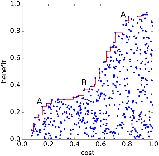
Figure 1. Schematic of a Pareto front (red line), with a function to be minimized (labeled “cost”) on the x−axis and a second function (labeled “benefit”), to be maximized, on the y−axis. Each blue dot represents a possible solution. The points along the Pareto front are Pareto-optimal solutions from which the benefit cannot be increased without increasing the cost; and cost cannot be reduced without reducing benefits. Convex sections of the front (“A”) represent locally preferred solutions. Concave sections (“B”) represent locally poorer solutions.

There is usually no single optimal solution. However the shape of the Pareto front gives information on solutions which may represent better, or preferred, choices. The center of convex frontal regions (“A” in Figure 1) represent better solutions where increased benefits require large cost increase, and cost can only be decreased with large reductions in benefit; while the center of concave regions (“B” in Figure 1) represent poorer solutions (Lester et al., 2013). Multi-objective approaches are always an enhancement over single-objective approaches; if automated return of a single solution is desired, then this is available by applying any desired single-objective function to those in the Pareto set; if not, a human decision maker, with input from stakeholders, can inspect the trade-off surface and make a well-informed decision (see Cabral et al., 2017 for a discussion of trade-off analysis). The Pareto front idea can be extended to optimizing more conditions, but becomes difficult to visualize; for example, with three functions the Pareto front will in general be a surface, and with N+1 functions the Pareto front could be N-dimensional.

For small networks we can examine all possible subnetworks, finding the optimal solutions by “brute force.” However, the number of possible subnetworks, 2^m, very quickly becomes unmanageably large. For larger networks we need an efficient search method to locate the Pareto-optimal solutions.

2.3. Search for Pareto Optimal Solutions

The broad field of optimization is concerned with efficiently finding good solutions to problems with non-trivial cost functions. With the exception of some special cases (such as minimal-spanning tree problems, or unconstrained linear systems), optimization algorithms do not guarantee finding true optima, but aim for the best solutions attainable in reasonable time, which in practice—when the algorithm is well-engineered for the problem at hand—tend to be either optimal or near-optimal. In the remainder of this section we will use “optimal” as shorthand for “optimal or near-optimal.”

A range of optimization methods are available, categorized in terms of the structural nature of the target problem. For example, when the problem can be formulated in terms of differentiable functions of real-valued parameters, “gradient methods” from mathematical optimization can be used (Snyman, 2005); when the problem can be formulated in terms of linear functions of discrete variables, methods from operations research can be used (Hillier and Lieberman, 2015). Although approaches exist to extend the reach of techniques from operations research and mathematical optimization, further categories of optimization method have wider applicability. Prominent among the latter are “metaheuristic” approaches (Voß et al., 1999; Glover and Kochenberger, 2003), which can be used to find optimal solutions in problems of arbitrary structure. To ensure that we do not constrain the cost-functions that may be used to evaluate MPA solutions, we design our algorithm from among the latter approaches.

Metaheuristic approaches are “black box” optimizers: the design of an algorithm does not rely on properties of the function(s) to be optimized; this is key to their wide applicability. A metaheuristic search process is guided primarily by the cost function values of solutions evaluated earlier in the process. A fundamental insight that guides search in metaheuristic algorithms is that solutions that are close in terms of their design parameters will often be close in terms of their cost function values; thus, in order to seek better solutions, it will be fruitful to sample new solutions close to the best ones found so far. Metaheuristic algorithms also devote some of their search effort to mechanisms that “explore” the search space by evaluating samples that are distant from the areas currently being exploited. Among the wide variety of metaheuristic approaches that could be applied, Markov Chain Monte Carlo (MCMC) frameworks provide arguably the most principled approach toward balancing exploitation and exploration. We therefore use ideas and methods from MCMC sampling to converge toward Pareto-optimal solutions from random initial estimates.

MCMC sampling centers on the concept of a “Markov Chain,” a sequence of connected “moves” through the sample space. In the current context, a “move” represents stepping from one MPA network A to another network B which is “close” to A; for example, A and B may share many sites in common. A sequence of such moves is often termed a (random) “walk.” In standard MCMC sampling, a walk is performed from a random starting position, and the new solution at each step along the walk is evaluated; steps along the walk may be rejected if they fail a stochastic test based on the cost/benefit values (in which case we stay at the current position and consider an alternative step). When MCMC is used for optimization (Strens, 2003; Lecchini-Visintini et al., 2010) (rather than for characterizing complex sample distributions; Gilks et al., 1995; Gamerman and Lopes, 2006), the stochastic test boosts the probability of moves toward high-quality regions of the search space. However the standard scheme often leads to slow or poor convergence since single chains can get trapped in suboptimal areas. An alternative approach is to use a collection of parallel walks to reduce the chance of suboptimal convergence (Craiu et al., 2009). We adopt this multiple walk approach, in part because it naturally promises highly effective speedup on parallel architectures, which may be necessary for large-scale MPA scenarios. In addition we repeatedly refresh these walks by restarting at positions on the best-so-far Pareto set; repeated restarts is common in parallel-walk MCMC algorithms (Martino et al., 2014; Garthwaite et al., 2016), while the idea of repeatedly exploiting the current approximation to the Pareto set borrows from prominent and successful “many-objective” optimization methods (Corne and Knowles, 2007). Finally, in our algorithm design we simplify the individual walks by omitting the use of a stochastic test, and simply accepting all moves along the walk. As we discovered in preliminary experiments, this was more successful than using a standard MCMC approach; although individual walks have an increased chance of wandering away from promising areas, this is balanced by the repeated restarts, which emphasise exploitation of the current Pareto set. We complete our description of the algorithm by describing details of the moves and structure, along with full pseudocode.

First consider possible choices of random steps. From any subnetwork we could take a step to any one of the other 2^m−1 subnetworks. A useful choice of step balances exploration of the local neighborhood with the ability to traverse the whole space in reasonable time. The simplest choice of step is the switching of a single randomly selected node between in and out of the network or vice versa. This fits our conditions: while allowing exploration of “nearby” space, a walker taking such steps could reach any subnetwork from any other in at most m steps. Computationally this also has the potential advantage of rapid evaluation of network metrics with just the addition or removal of a single node. This will be our random step, the node to switch is selected using a uniformly distributed random number.

Second, to maintain pressure toward encountering solutions that will advance beyond the current Pareto set, we need to keep our random walkers in the vicinity of the better solutions found so far. In a preliminary version of the algorithm we used the recognized MCMC optimization approach in which a move was only accepted if it passed a stochastic test. However, in our final algorithm design, every move in a walk is accepted, and the pressure toward optimal solutions instead comes from the multiple walker framework, as described next.

The algorithm operates by running repeated series of parallel but independent random walks. Initially, a simple random search is done to obtain an initial Pareto set of solutions. Then, starting from a subset of these solutions, k independent random walks are launched, each lasting for s steps, updating the current Pareto set according to the solutions evaluated along the way. This set of independent random walks is repeated, each time starting each walk from a randomly selected sample in the current Pareto set, until a termination criterion is reached. Effectively, the dynamically changing Pareto set acts to repeatedly select, prune or “multiply” search trajectories. Trajectories that did not contribute the Pareto set become “pruned,” those that do contribute may be multiplied.

Note that while this method must converge eventually, there is no guarantee that it converges to the correct, global, Pareto optimal solutions. Use of a larger set of initial random subnetworks, and more steps, s, in each walk reduces the chance of converging to a locally optimal solution. The efficiency of the method relies on the use of well-behaved, rather than noisy, optimization functions which vary slowly with choice of nodes in the subnetwork.

2.4. Cost Functions

To examine the use of connectivity in network optimization, we use a connectivity-based objective function—a proxy for network resilience and gene flow—and a simple site-based cost function. The merits of these objective functions and further possible choices of function are discussed in section 4.

2.4.1. Costs

For the model networks (section 2.5) and the decommissioning example (section 2.6.2) sites are considered to have equal cost so a network of k sites has a cost of k.

MPA network proposals often include industry-based estimates of financial costs to fishing, shipping, renewable energy, oil and gas, and mining industries. For the Scottish MPA network (section 2.6.1) these costs are available from the Business and Regulatory Impact Assessments (BRIAS) conducted as part of the Scottish Government MPA consultation (http://www.gov.scot/Topics/marine/marine-environment/mpanetwork) or Impact Assessments produced for consideration as a Special Area of Conservation (SAC) under the EU Habitats Directive 1992 (http://jncc.defra.gov.uk/page-4524). Here we use estimates of ongoing management costs and costs to the fishing industry from these Impact Assessments as most relevant to the protection of Lophelia pertusa. Upper cost estimates to fishing were used, representing the removal of all bottom-contacting fishing from protected sites. Where such estimates were not available (Hatton Bank, North West Rockall Bank and South East Rockall Bank), an estimate from a similar nearby site was used, weighted by site area. To these we add an average annual management cost, obtained from the SAC Impact Assessments, of £50,000 per year for each site. We do not claim these costs as complete or authoritative, a rigorous cost analysis would be required in a practical application. The estimated costs here cover a realistic range and serve to demonstrate the optimization method.

In the North Sea decommissioning example (section 2.6.2) minimum financial cost and maximum network connectivity may both be achieved by leaving all platforms in place. But this solution could have reputational costs to government and industry: under Decision OSPAR 98/3 Disposal of Disused Offshore Installations for parties contract to the OSPAR Convention, all topsides and substructure are to be fully removed with few exceptions for derogation. Policy change to leave installations in place could be perceived as motivated by cost-cutting rather than environmental concerns. Additionally, leaving installations in place, either wholly or partially, could restrict the opportunity for growth in the fisheries industry, so it is reasonable to consider the number of installations left in the network as a “cost” to be minimized.

2.4.2. Benefits

Average shortest path, the smallest distance to travel between any two sites in a network averaged over all pairs of sites, is one of a suite of network metrics used as indicators of network robustness (Watts and Strogatz, 1998; Manzano et al., 2015). Also used to characterize “small world” networks and interconnectedness (Albert et al., 2000), ecologically, the average shortest path gives an idea of the gene flow through a network, increased gene flow can promote adaptation (Tigano and Friesen, 2016). Here, the average shortest path metric is calculated for each protected subnetwork G_S being considered. To avoid only selecting for the smallest fully connected networks (two nodes with a connection in both directions), we make small modifications to the standard average shortest path calculation. Firstly, we calculate the average shortest path over all the pairs of sites in the full network G_T, having first removed all connections into and out of nodes which are not in the protected subnetwork G_S. This assumption could be relaxed to instead reduce the weight of connections to and from unprotected sites (see for example Nilsson Jacobi and Jonsson, 2011). Secondly, if there is no possible path between a pair of nodes we define the shortest path to be D, longer than the distance across the full network. Finally, in the real-world examples we include self-connections in the shortest path lengths, these represent return of larvae to the source site.

We include edge weights in the average shortest path, where the edge e_ij, from x_i to x_j, has weight w_ij and corresponding length d_ij. The edge length is calculated directly for the model networks as described in section 2.5. For the real-world networks the larval connectivity modeling gives estimates of the relative probability of a link between any two sites, i.e., edge weights w_ij, where 0 ≤ w_ij < 1. Weights are converted to distances using

this maintains the natural interpretation of the probability of a link along a chain

2.5. Model Networks

Various graph models have been used in studies of marine connectivity. Kininmonth et al. (2011) explores many types including minimally connected, nearest neighbor, small-world, geometric, random, and scale free graphs. Considering the physical processes underlying benthic ecological networks we use a modification of random geometric graphs (Penrose, 2003). Random geometric graphs have nodes randomly distributed in geometric space with connections between pairs of nodes separated by less than a specified distance. Benthic subpopulations can appear to be randomly distributed, although distribution is governed by water depths, substrates, local watermass properties, hydrodynamics, food and nutrient delivery, and human pressures. The fixed radius of connections in random geometric graphs models turbulent transport and random swimming of pelagic larvae in the absence of mean flows. Here we refine the definition to introduce a directional bias to the connections, analogous to the common situation of populations within a mean flow. The advantage of model graphs is we can control size and connectivity of the network for a thorough test of the search and optimization methods.

While this form of graph is chosen primarily to model the common form of sessile benthic species with a pelagic larval phase and a metapopulation/subpopulation structure, similar model graphs—which consist purely of nodes and weighted connecting edges—could easily be constructed to represent species with direct development or continuous distribution. The optimization approach described is general and applicable to any network configuration.

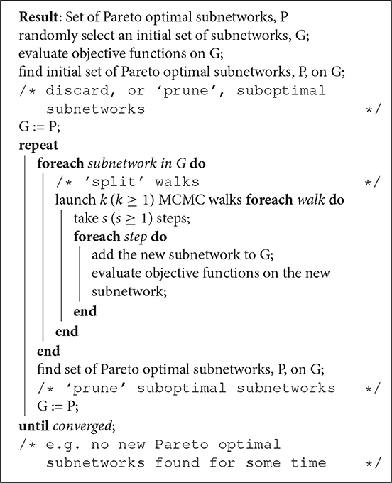
We construct such graphs, G_T(V_T, E_T), (Figure 2) with nodes, V_T, and edges, E_T, in 2-d geometric, (x, y), space. Here m nodes were positioned randomly on the plane x ∈ [0, 1], y ∈ [0, 1]. With spreading distance r (in time t) and uniform flow u, with associated displacement s in time t (in the positive x−direction) each node (x_i, y_i) was connected to all nodes (x_j, y_j) according to

Each node (x_i, y_i) is connected to all other nodes (x_j, y_j) that lie within distance r of the point (x_i+s, y_i). The separation length d_ij is the distance from the spreading center (x_i+s, y_i) to node (x_j, y_j). That is

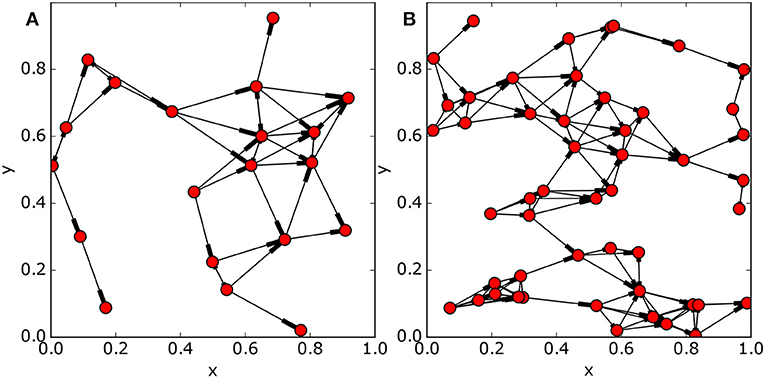
Figure 2. Modified random geometric networks of 20 nodes (A) and 50 nodes (B). Edge connections are toward the thickened end of the line. Parameters used in the construction: (a) m = 20, r = 0.17, s = 0.085; (b) m = 50, r = 0.15, s = 0.085.

2.6. Example Real-World Networks

Two real-world cases are tested: the Scottish MPA network and a man-made network of oil and gas installations in the North Sea, with connectivity matrices derived from larval dispersal modeling (Fox et al., 2016).

2.6.1. Scottish MPA Network

In Scottish waters MPAs have been designated for the protection of cold-water coral L. pertusa (Roberts et al., 2006). The weighted larval connections have been modeled by Fox et al. (2016), Figure 3. This is a small network of 12 sites so we can easily evaluate objective functions for all possible network configurations, finding the true Pareto optimal solutions by brute force. Estimates of costs for each site, determined as described in section 2.4.1 are shown in Table 1.

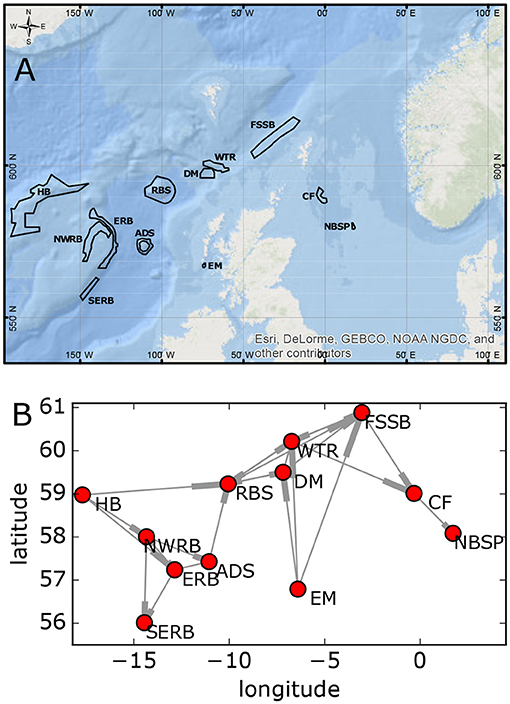
Figure 3. Estimated connectivity of Scottish MPA network for L. pertusa from Fox et al. (2016). (A) Map of the network. (B) Diagram of the connectivity. Connection direction is toward the thickened end of the edge. Site name abbreviations are listed in Table 1.

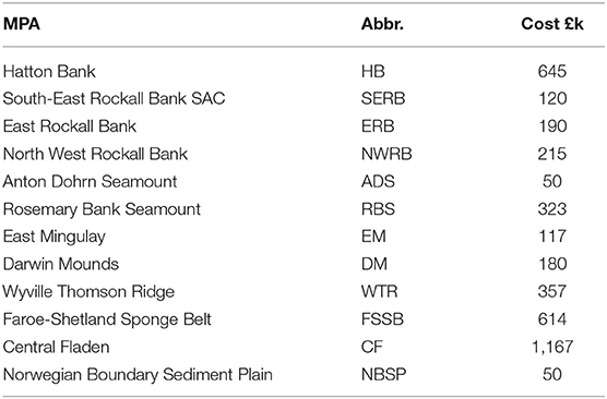
Table 1. Estimated annual costs associated with Scottish MPAs (thousands of £).

2.6.2. North Sea Oil and Gas Installation Decommissioning Scenario

Within the North Sea, oil and gas platforms form a man-made network providing hard substrates generally unavailable in the North Sea away from the coasts. These platforms are colonized by benthic species (Roberts, 2002) including hard corals (L. pertusa), soft corals (Alcyonium digitatum), mussels (Mytilus edulis), barnacles (Chirona hameri) and anemones (Metridium sessile). Many installations are reaching the decommissioning stage, so work is ongoing to quantify the contribution of this man-made network to North Sea biodiversity and interconnectedness of this new man-made ecosystem (Henry et al., 2018). It is interesting therefore to examine scenarios where some of the substructure is left in place to form artificial reefs of hard substrate ecosystems.

Particle tracking experiments simulating larval connectivity among the installations were done using the Lagrangian TRANSport model (LTRANSv.2b, North et al., 2011) with a high resolution configuration of the Nucleus for European Modeling of the Ocean (NEMO) for the North West European Shelf, the NEMO-AMM60 (Atlantic Margin Model 1/60 degree, Guihou et al., 2018). Here, 100 particles were released daily during 14 days (February 15 to 28, 2010) at the location of each installation and tracked for 40 days, near the upper limit of the pelagic larval duration for the shallow-water species observed on North Sea oil platforms. Particle trajectories were evaluated for settlement inside 1 km diameter circular polygons centerd at the subsea structures. The full network consists of over 1,000 installations, too many for the optimization method to converge in reasonable time, so we consider a gridded network of 104, 0.5 × 0.5 degree areas (Figure 4). Connections and connection weights in the gridded network are accumulated from the connections between all pairs of platforms in each grid cell.

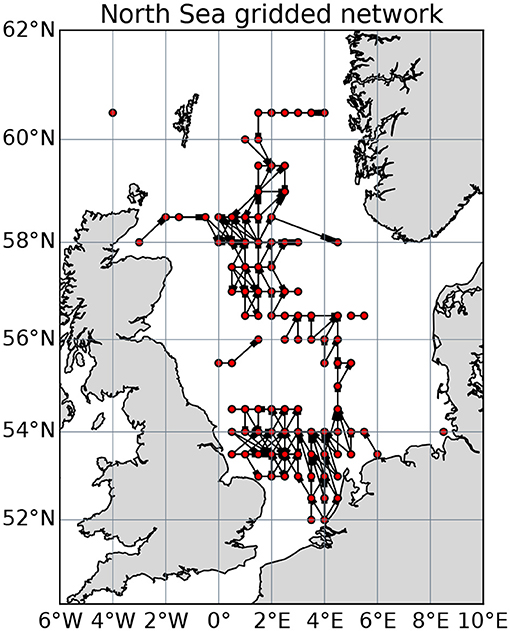
Figure 4. The network of connected North Sea oil and gas installations gridded at 0.5 by 0.5 degrees. Directed connections are thickened in the direction of travel.

All methods were implemented in python in Jupyter notebooks, an example is included as Supporting Information. Graph theory metrics were calculated using the networkX package and results plotted using the matplotlib package.

3. Results

First we show the multivariate optimization for small networks where we can use brute force to examine all possible networks, and then we test the more efficient search method and using it to examine two larger networks.

3.1. Small Networks—Brute Force

Figure 5 shows the Pareto optimal solutions for the 20-node model network in Figure 2. The Pareto front (Figure 5A) has a uniform slope (away from the extremes) suggesting no optimal solutions are to be preferred over others (final selection would require a decision maker and stakeholder input). Figure 5B shows the make-up of each optimal solution, highlighting which nodes are included. Each optimal solution is built around a core of the best connected nodes, gradually expanding with the addition of nodes as costs are increased, with the poorly connected sites on the edges selected last (maps of all optimal networks are included in Supporting Information). Figure 5C shows that for each possible network size a single optimal network has been identified, except for single node solutions where none are optimal. The use of at least one optimization function that does not return identical values for any two distinct network configurations ensures the uniqueness of each optimal solution.

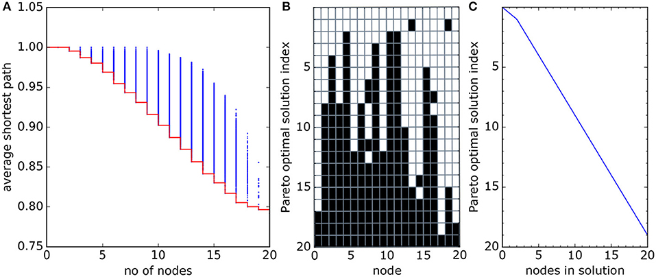
Figure 5. (A) All possible cost/average shortest path function pairs (“solutions,” blue dots) for the network in Figure 2A. The Pareto optimal solutions lie on the red line. (B) Node structure of the Pareto optimal solutions. Each row represents an optimal subnetwork, each column a network node. Black filled squares are nodes included in the optimal subnetwork. The “Pareto optimal solution index” (y-axis) is a numbering of the optimal subnetworks, from smallest (single node) to largest (full network), used in the text to refer to individual solutions. The network sizes are shown in (C). Data for this plot were found by brute force, examining all 2²⁰ = 1, 048, 576 possible networks.

The Scottish MPA network uses a node-dependent cost function and also includes larval retention (or “self-loops”) in the analysis (Figure 6). The Pareto front is less smooth than for the model networks, and the inclusions of a variable cost function produces many more points on the front. We note from Figure 6A that firstly, the bulk of the possible networks lie far from the optimal solutions, and secondly, changes in gradient of the Pareto front can be used to identify locally “preferred” optimal solutions, as described in section 2.3. These are the solutions that would be most valued by decision-makers. The structure of four of these preferred optimal subnetworks, are shown in Figure 7. The preferred optimal subnetworks are built around a central core of nodes, excluding those on the periphery. This central core of nodes begins with Anton Dohrn Seamount (ADS), East Rockall Bank (ERB), North West Rockall Bank (NWRB), and South East Rockall Bank (SERB) before expanding northeastwards to include Rosemary Bank Seamount (RBS), Darwin Mounds (DM) and Wyville Thomson Ridge. The inclusion of Norwegian Boundary Sediment Plain (NBSP) in these “preferred” solutions is interesting. Even though it is unconnected to the other protected sites it is included because it is low-cost and retains a significant proportion of the larvae it produces, thus adding to overall network resilience. The priority for protection suggested by these “preferred” results is based on a mix of cost and connectivity.

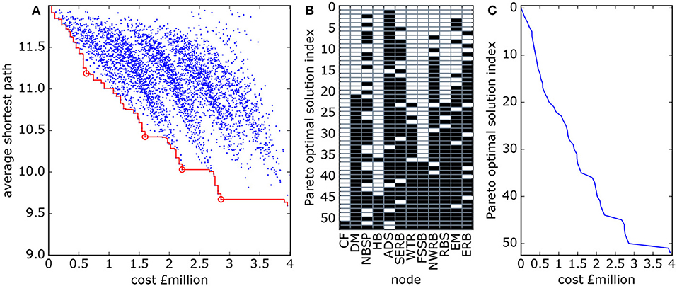
Figure 6. (A) Cost and average shortest path length for all subnetworks of the Scottish MPA network shown in Figure 3 (blue dots). The red line links the Pareto optimal points. The open circles indicate the locally “better” solutions—lower cost and shorter average shortest path—on the Pareto front. Panels (B,C) are the composition (B) and cost (C) of the Pareto optimal subnetworks as described for Figure 5. Site name abbreviations (x-axis in B) are listed in Table 1.

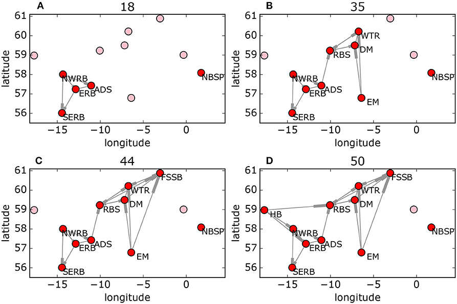
Figure 7. Four of the “preferred” Pareto-optimal solutions (indicated by the circles in Figure 6A) for the Scottish MPA network (Figure 3) in order of increasing cost (A–D). Red and pink circles show sites included in and excluded from the network, respectively.

3.2. Larger Networks—Metaheuristic Search

For larger networks we use the metaheuristic search. First we tested this method to recalculate the optimal solutions for the small networks in section 3.1. In all cases the true global optimal solution was reached in much reduced time (results for the 20-node model network are in Supporting Information). For the 20-node model networks, the correct solution is reached while examining fewer than 0.005% of the possible solutions. The efficiency savings increase with network size.

The results of the optimal solution search for the 50-node network (Figure 2B) are shown in Figure 8. The search was ended when no new optimal solutions had been found for 100 iterations, when only 65,000 of a possible 2⁵⁰ solutions had been examined. It is not possible to prove that this is the correct solution, but it passes some simple checks, the set of optimal solutions found is unaffected by the initial random selection.

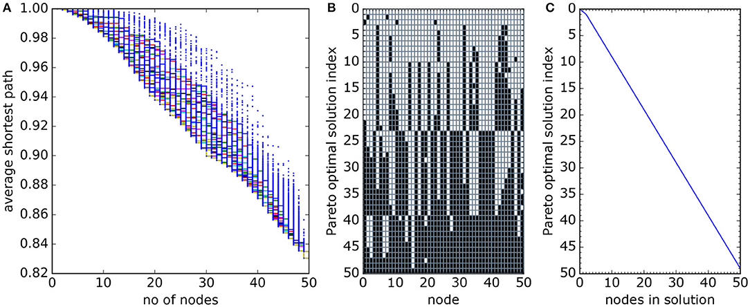
Figure 8. Estimated Pareto front for the 50-node network. (A) Successive iterative estimates of the Pareto front (solid colored lines) with blue dots showing computed values of average shortest path for each network. (B) The structure of the Pareto optimal solutions and, (C) the number of nodes in each Pareto optimal solution. Notice the region of slightly “better” (convex front shape in A) solutions around 30 nodes and the sharp changes in structure of the 50-node Pareto optimal solution between solution index numbers 22 and 23, and again between 38 and 39 in panel (B).

The set of optimal solutions has features which were not observed in the smaller networks. Most notably, a step change in the structure of the network is visible in Figure 8B between Pareto optimal solutions with index numbers 22 and 23, with most of the protected nodes in solution number 22 being unprotected in solution 23. There is a second smaller such step change between solutions index 38 and 39. The full network has two well-connected clusters, one for nodes with y > 0.4 and the other for y < 0.4. The cluster of sites with smaller y values (“southern” sites) is better connected but smaller – so the smaller optimal networks are selected from these sites. But there is a tipping point at 23 sites, where there are no more southern sites to select. Rather than adding northern sites to the southern network, the whole optimal network switches to the northern cluster (Figures 9A,B).

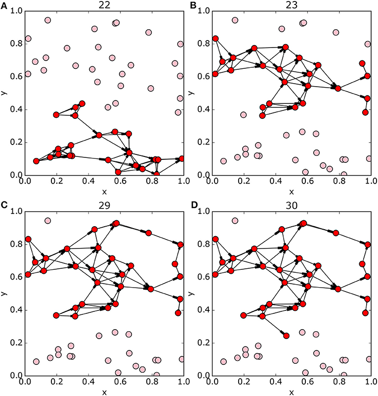
Figure 9. Pareto-optimal subnetworks, bright red nodes are included in the network, light red are excluded. Panels (A,B) show the networks either side of the subnetwork structural discontinuity at solution 22 in Figure 8B. There is a step change in optimal network structure with the addition of just a single site to the optimal solution, from exclusively “southern” sites (y < 0.4) to exclusively on “northern” sites (y > 0.4). Panels (C,D) show the optimal subnetworks around the change in gradient in the Pareto front at 29 nodes (Figure 8A). Subnetworks of more than 30 nodes must include sites from both the “northern” and “southern” groups and the average shortest path improves more slowly.

Also observe the change in gradient of the front at 29–30 protected nodes (Figure 8A), here the addition of a few more protected nodes causes relatively little improvement in average shortest path. This occurs as the subnetwork of northern nodes is complete and further network expansion requires inclusion of sites on both sides of the weak connection around y = 0.4 (Figures 9C,D).

Figure 10 shows results for the real-world network of oil and gas installations in the North Sea (section 2.6.2). A stable set of Pareto optimal solutions here was obtained by examining about 250,000 of the possible 2¹⁰⁴ solutions.

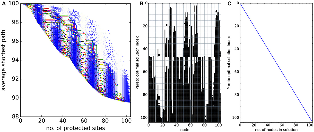
Figure 10. As Figure 8 for the network of oil and gas installations in the North Sea, Figure 4. (A) Estimates of the Pareto front. (B) The Pareto optimal solutions and, (C) the number of nodes in each Pareto optimal solution. The estimate of the Pareto optimal solutions here was found by examining 250, 000 of the possible 2¹⁰⁴ subnetworks. Notice the step change in Pareto optimal subnetwork structure, visible around solution index 45 to 47 in panel (B). The optimal subnetworks around this index are illustrated in Figure 11.

This real-world set of Pareto optimal solutions contains many of the features described for the model network: a step change in structure (at solution number 45, Figure 10B) and locally preferred solutions (convex front around 40 and 75 sites, Figure 10A). The step change is again caused by northern and southern networks with poor connections between, the optimal subnetwork doesn't switch fully between clusters with increasing size, but switches from entirely southern sites to a combination of southern and northern sites (Figure 11). The preferred solutions at around 40 protected sites (Figure 10A) occur just before this step change. The slow-down in average shortest path improvement as more sites are protected after 75 sites occurs because the remaining unprotected sites are poorly-connected peripheral sites.

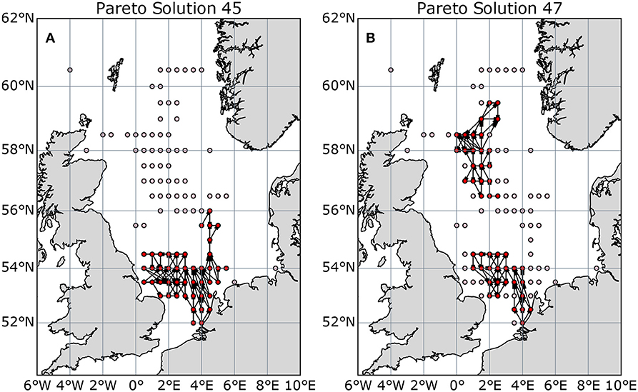
Figure 11. Selected Pareto-optimal subnetworks of the North Sea gridded network, either side of the structural discontinuity at solution 45–47 (45–47 nodes protected) in Figure 10B. (A) optimal solution with 45 nodes protected; (B) 47 nodes protected. Bright red nodes are included in the subnetwork, light red are excluded.

4. Discussion

We have demonstrated the effectiveness and advantages of multivariate optimization of the selection of sites in networks of MPAs and man-made structures based on Pareto optimal sets. Such methods allow examination of trade-offs to inform decision-making. As the number of possible network configurations grows very rapidly with network size, an efficient method of estimating the set of optimal solutions is required. We take a metaheuristic approach, suited to problems of arbitrary cost function structure, to ensure that we do not limit or constrain the potential cost-functions that may be used to evaluate MPA solutions.

The multivariate optimization locates step changes in the structure of the optimal network for small variations in cost functions. These step changes were not observed in the shape of the Pareto front, but require examination of the optimal subnetwork structure. In theory the optimal subnetwork of n+1 sites may be quite different from that of n sites, the present study demonstrates that this is a common eventuality.

The methods also allow identification of “preferred” optimal solutions, particularly with larger networks and more detailed cost functions. These are solutions where increasing cost (or adding sites) produces minimal increase in benefit, and cost cannot be reduced (more sites unprotected) without a disproportionately large reduction in benefit. This identification of gradients in objective function trade-off space is a clear advantage of the multi-criteria approach.

While the optimization approach is suited to arbitrary cost function structure, the results described are based on a specific pair of objective functions: a simple site-based economic cost function and a connectivity-based function—the average shortest path. These functions were chosen for their relevance to the real-world cases considered, design of networks for protection of long-lived benthic populations where the primary threats are catastrophic anthropogenic damage.

The model and real-world examples presented are based on benthic species with sessile adult phase and at least partially pelagic larval phase. This choice was motivated by problems of conservation and management in the deep sea where this life-cycle is thought to be ubiquitous, although the method is more generally applicable. Deep-sea benthic sediment communities are dominated by polychaetes, crustaceans, molluscs and echinoderms, with cnidarians and sponges dominant on hard substrates (Gage and Tyler, 1991). Young (2003) reviews the knowledge of embryogenesis and larval development of these groups in the deep sea. The most common larval life history pattern in all groups is thought to contain a pelagic phase of some length (Pechenik, 1999), either lecithotropic (not feeding, generally shorter duration) or planktotrophic (feeding, generally longer duration). Bradbury et al. (2008) also reviews data on marine fishes, including deep sea species, where again the most common life history includes a pelagic larval phase.

The use of average shortest path here as a proxy for network resilience is a simplification of the ecosystem and metapopulation dynamics. However, the results closely support the conclusions of other work based on more detailed metapopulation persistence models. Kininmonth et al. (2011) found that for network persistence, protection needs to prioritize “hubs” or “clusters” with high connectivity. The optimization results of Nilsson Jacobi and Jonsson (2011) suggest a similar strategy, but they imposed an arbitrary limit on the number of sites in each “cluster” to be protected, resulting in a wider distribution of sites in their optimal solution. Hastings and Botsford (2006) show theoretically that only patterns of reproduction and connectivity which eventually lead to descendants returning to the patch from which they originate contribute to persistence. The results from the average shortest path proxy used here support this idea that such “strongly connected” clusters are given priority. The use of a weighted shortest path metric and inclusion of self-connections suggests optimal networks may contain isolated sites where large numbers of larvae are retained.

While these comparisons provide support for the use of average shortest path as a proxy for network persistence, connectivity is only part of metapopulation dynamics, and the aim of conservation planning is to ensure metapopulation persistence across a range of species (Kininmonth et al., 2011). Connectivity data must be used together with other data. Connectivity does not represent habitat quality, diversity of habitat types, and species diversity, among other factors. A focus on high connectivity doesn't necessarily ensure persistence and might decrease resilience if it leads to clumped networks on spatial scales analogous to disturbance scales (Game et al., 2008; Levin and Lubchenco, 2008; Almany et al., 2009).

We also assume throughout that connectivity is constant in time, even though on short timescales stochasticity in connectivity patterns in marine systems is common (Hogan et al., 2012; Fox et al., 2016) and on multi-decadal timescales the circulation of the North Sea could change (Holt et al., 2018). While this constant in time assumption is probably appropriate for the species considered here—benthic species with lifespans that are long compared to the dominant short-term variability of the currents but short compared to the climatic variability of the currents—it may be less valid for short-lived fish species or for connectivity in future climate scenarios.

The current work considers optimization of a network for a single species in isolation, in practice marine conservation is still often based around these individual, often vulnerable, habitat-forming, species (for example the Scottish MPA process above). In such cases, the full, unconstrained, multi-objective optimization approach would provide important information to help guide conservation planning when considered alongside other data and input from stakeholders and planning decision-makers. It must be stressed that the multiobjective optimization and search methods described are completely independent of the choice of objective functions.

Alternative objective functions could be based on meta-population or meta-community models incorporating species-species interactions and many factors determining population persistence, including stochastic effects (Hanski and Gilpin, 1991; Guichard et al., 2004). The major difficulty using these models in multiobjective optimization is the computational load incurred by the need to run the model on many subnetworks.

Additional objective functions can also easily be added to the optimization as Pareto-optimal solutions can be also calculated for more than two functions. The disadvantages are that the front becomes difficult to visualize and many more Pareto optimal points will typically exist, slowing the search. The addition of further functions could be used to extend the method to multiple species (with individual connectivity matrices), or include factors such as network spatial scale, or site-based habitat quality measures. These extensions are beyond the scope of the current work and will be the subject of further studies.

Data Availability Statement

The raw data supporting the conclusions of this manuscript will be made available by the authors, without undue reservation, to any qualified researcher.

Author Contributions

AF, DC, JR, L-AH, and JP conceived the ideas. AF and DC designed the methodology. JP, CM, and AF produced the connectivity matrices used for the real-world cases. AF led the writing of the manuscript. All authors contributed critically to the drafts and gave final approval for publication.

Funding

AF was supported by a Daphne Jackson Fellowship. All authors acknowledge support from the ANChor project funded through the INSITE programme. This work is a contribution to the ATLAS project and has received funding from the European Union's Horizon 2020 research and innovation programme under grant agreement no. 678760. The paper reflects the authors' views and the European Union is not responsible for any use that may be made of the information it contains.

Conflict of Interest Statement

The authors declare that the research was conducted in the absence of any commercial or financial relationships that could be construed as a potential conflict of interest.

Acknowledgments

AF would like to acknowledge Prof. Mathew Penrose (University of Bath) for discussions about random geometric graphs.

Supplementary Material

The Supplementary Material for this article can be found online at: https://www.frontiersin.org/articles/10.3389/fmars.2019.00017/full#supplementary-material

References

Albert, R., Jeong, H., and Barabasi, A.-L. (2000). Error and attack tolerance of complex networks. Nature 406, 378–382. doi: 10.1038/35019019
Almany, G. R., Connolly, S. R., Heath, D. D., Hogan, J. D., Jones, G. P., McCook, L. J., et al. (2009). Connectivity, biodiversity conservation and the design of marine reserve networks for coral reefs. Coral Reefs 28, 339–351. doi: 10.1007/s00338-009-0484-x
Andrello, M., Mouillot, D., Somot, S., Thuiller, W., and Manel, S. (2015). Additive effects of climate change on connectivity between marine protected areas and larval supply to fished areas. Divers. Distrib. 21, 139–150. doi: 10.1111/ddi.12250
Ball, I. R., Possingham, H. P., and Watts, M. E. (2009). “Marxan and relatives: software for spatial conservation prioritization,” in Spatial Conservation Prioritisation: Quantitative Methods and Computational Tools, eds A. Moilanen, K. A. Wilson, and H. P. Possingham (Oxford: Oxford University Press), 185–195.
Berglund, M., Nilsson Jacobi, M., and Jonsson, P. R. (2012). Optimal selection of marine protected areas based on connectivity and habitat quality. Ecol. Modell. 240, 105–112. doi: 10.1016/j.ecolmodel.2012.04.011
Botsford, L. W., Hastings, A., and Gaines, S. D. (2001). Dependence of sustainability on the configuration of marine reserves and larval dispersal distance. Ecol. Lett. 4, 144–150. doi: 10.1046/j.1461-0248.2001.00208.x
Bradbury, I. R., Laurel, B., Snelgrove, P. V. R., Bentzen, P., and Campana, S. E. (2008). Global patterns in marine dispersal estimates: the influence of geography, taxonomic category and life history. Proc. Biol. Sci. 275, 1803–1809. doi: 10.1098/rspb.2008.0216
Burgess, S. C., Nickols, K. J., Griesemer, C. D., Barnett, L. A., Dedrick, A. G., Satterthwaite, E. V., et al. (2014). Beyond connectivity: How empirical methods can quantify population persistence to improve marine protected-area design. Ecol. Appl. 24, 257–270. doi: 10.1890/13-0710.1
Cabral, R. B., Gaines, S. D., Lim, M. T., Atrigenio, M. P., Mamauag, S. S., Pedemonte, G. C., et al. (2016). Siting marine protected areas based on habitat quality and extent provides the greatest benefit to spatially structured metapopulations. Ecosphere 7:e01533. doi: 10.1002/ecs2.1533
Cabral, R. B., Halpern, B. S., Costello, C., and Gaines, S. D. (2017). Unexpected management choices when accounting for uncertainty in ecosystem service tradeoff analyses. Conserv. Lett. 10, 422–430. doi: 10.1111/conl.12303
Carroll, C., McRae, B. H., and Brookes, A. (2012). Use of linkage mapping and centrality analysis across habitat gradients to conserve connectivity of Gray Wolf populations in Western North America. Conserv. Biol. 26, 78–87. doi: 10.1111/j.1523-1739.2011.01753.x
Carson, H. S., Levin, L. A., Cook, G. S., López-Duarte, P. C., and Levin, L. A. (2011). Evaluating the importance of demographic connectivity in a marine metapopulation. Ecology 92, 1972–1984. doi: 10.1890/11-0488.1
Corne, D. W., and Knowles, J. D. (2007). “Techniques for highly multiobjective optimisation: some nondominated points are better than others,” in Proceedings of the 9th Annual Conference on Genetic and Evolutionary Computation - GECCO '07 (New York, NY: ACM Press), 773. doi: 10.1145/1276958.1277115
Cowen, R. K., and Sponaugle, S. (2009). Larval dispersal and marine population connectivity. Annu. Rev. Mar. Sci 1, 443–466. doi: 10.1146/annurev.marine.010908.163757
Craiu, R. V., Rosenthal, J., and Yang, C. (2009). Learn from thy neighbor: parallel-chain and regional adaptive MCMC. J. Am. Stat. Assoc. 104, 1454–1466. doi: 10.1198/jasa.2009.tm08393
Foster, N. L., Paris, C. B., Kool, J. T., Baums, I. B., Stevens, J. R., Sanchez, J. A., et al. (2012). Connectivity of Caribbean coral populations: complementary insights from empirical and modelled gene flow. Mol. Ecol. 21, 1143–1157. doi: 10.1111/j.1365-294X.2012.05455.x
Fox, A. D., Henry, L.-A., Corne, D. W., and Roberts, J. M. (2016). Sensitivity of marine protected area network connectivity to atmospheric variability. R. Soc. Open Sci. 3:160494. doi: 10.1098/rsos.160494
Gage, J. D., and Tyler, P. A. (1991). Deep-Sea Biology: A Natural History of Organisms at the Deep-Sea Floor. Cambridge: Cambridge University Press.
Game, E. T., Watts, M. E., Wooldridge, S., and Possingham, H. P. (2008). Planning for persistence in marine reserves: a question of catastrophic importance. Ecol. Appl. 18, 670–680. doi: 10.1890/07-1027.1
Gamerman, D., and Lopes, H. F. (2006). Markov Chain Monte Carlo : Stochastic Simulation for Bayesian Inference. Boca Raton, FL: Chapman and Hall/CRC.
Garthwaite, P. H., Fan, Y., and Sisson, S. A. (2016). Adaptive optimal scaling of MetropolisHastings algorithms using the RobbinsMonro process. Commun. Stat. Theor. Methods 45, 5098–5111. doi: 10.1080/03610926.2014.936562
Gilks, W. R., Richardson, S., and Spiegelhalter, D. J. (1995). Markov Chain Monte Carlo in Practice eds W. R. Gilks, S. Richardson, and D. J. Spielgelhalter (Boca Raton, FL: Chapman & Hall/CRC).
Glover, F., and Kochenberger, G. A. (2003). Handbook of Metaheuristics. New York, NY: Kluwer Academic Publishers.
Guichard, F., Levin, S., Hastings, A., and Siegel, D. A. (2004). Toward a dynamic metacommunity approach to marine reserve theory. Bioscience 54, 1003–1011. doi: 10.1641/0006-3568(2004)054[1003:TADMAT]2.0.CO;2
Guihou, K., Polton, J., Harle, J., Wakelin, S., O'Dea, E., and Holt, J. (2018). Kilometric scale modeling of the North West European Shelf seas: exploring the spatial and temporal variability of internal tides. J. Geophys. Res. Oceans 123, 688–707. doi: 10.1002/2017JC012960
Hanski, I., and Gilpin, M. E. (1991). Metapopulation Dynamics: Empirical and Theoretical Investigations. London: Academic Press.
Hastings, A., and Botsford, L. W. (2006). Persistence of spatial populations depends on returning home. Proc. Natl. Acad. Sci. U.S.A. 103, 6067–6072. doi: 10.1073/pnas.0506651103
Henry, L.-A., Mayorga Adame, C. G., Fox, A. D., Polton, J. A., Ferris, J. S., McLellan, F., et al. (2018). Ocean sprawl facilitates dispersal and connectivity of protected species. Sci. Rep. 8:11346. doi: 10.1038/s41598-018-29575-4
Hillier, F. S., and Lieberman, G. J. (2015). Introduction to operations research. New York, NY: McGraw-Hill Education.
Hogan, J. D., Thiessen, R. J., Sale, P. F., and Heath, D. D. (2012). Local retention, dispersal and fluctuating connectivity among populations of a coral reef fish. Oecologia 168, 61–71. doi: 10.1007/s00442-011-2058-1
Holt, J., Polton, J., Huthnance, J., Wakelin, S., ODea, E., Harle, J., et al. (2018). Climate-driven change in the North Atlantic and Arctic Ocean can greatly reduce the circulation of the North Sea. Geophys. Res. Lett. 45, 11827–11836. doi: 10.1029/2018GL078878
James, M. K., Armsworth, P. R., Mason, L. B., and Bode, L. (2002). The structure of reef fish metapopulations: modelling larval dispersal and retention patterns. Proc. Biol. Sci. R. Soc. 269, 2079–2086. doi: 10.1098/rspb.2002.2128
Jonsson, P. R., Nilksson Jacobi, M., and Moksnes, P.-O. (2016). How to select networks of marine protected areas for multiple species with different dispersal strategies. Divers. Distrib. 22, 161–173. doi: 10.1111/ddi.12394
Kininmonth, S., Beger, M., Bode, M., Peterson, E., Adams, V. M., Dorfman, D., et al. (2011). Dispersal connectivity and reserve selection for marine conservation. Ecol. Modell. 222, 1272–1282. doi: 10.1016/j.ecolmodel.2011.01.012
Lecchini-Visintini, A., Lygeros, J., and Maciejowski, J. M. (2010). Stochastic optimization on continuous domains with finite-time guarantees by Markov Chain Monte Carlo Methods. IEEE Trans. Automat. Control 55, 2858–2863. doi: 10.1109/TAC.2010.2078170
Lehtomäki, J., and Moilanen, A. (2013). Methods and workflow for spatial conservation prioritization using Zonation. Environ. Modell. Softw. 47, 128–137. doi: 10.1016/j.envsoft.2013.05.001
Leslie, H. M. (2005). A synthesis of marine conservation planning approaches. Conserv. Biol. 19, 1701–1713. doi: 10.1111/j.1523-1739.2005.00268.x
Lester, S. E., Costello, C., Halpern, B. S., Gaines, S. D., White, C., and Barth, J. A. (2013). Evaluating tradeoffs among ecosystem services to inform marine spatial planning. Mar. Policy 38, 80–89. doi: 10.1016/j.marpol.2012.05.022
Levin, S. A., and Lubchenco, J. (2008). Resilience, robustness, and marine ecosystem-based management. Bioscience 58, 27–32. doi: 10.1641/B580107
Lopez-Duarte, P. C., Carson, H. S., Cook, G. S., Fodrie, F. J., Becker, B. J., Dibacco, C., et al. (2012). What controls connectivity? An empirical, multi-species approach. Integr. Comp. Biol. 52, 511–524. doi: 10.1093/icb/ics104
Magris, R. A., Treml, E. A., Pressey, R. L., and Weeks, R. (2016). Integrating multiple species connectivity and habitat quality into conservation planning for coral reefs. Ecography 39, 649–664. doi: 10.1111/ecog.01507
Manzano, M., Sahneh, F., Scoglio, C., Calle, E., and Marzo, J. L. (2015). Robustness surfaces of complex networks. Sci. Rep. 4:6133. doi: 10.1038/srep06133
Martino, L., Elvira, V., Luengo, D., Artés-Rodríguez, A., and Corander, J. (2014). Orthogonal MCMC algorithms. 2014 IEEE Workshop Stat. Signal Process. 364–367.
Miettinen, K. (1999). Nonlinear Multiobjective Optimization. Boston, MA: Kluwer Academic Publishers.
Moilanen, A., Anderson, B. J., Eigenbrod, F., Heinemeyer, A., Roy, D. B., Gillings, S., et al. (2011). Balancing alternative land uses in conservation prioritization. Ecol. Appl. 21, 1419–1426. doi: 10.1890/10-1865.1
Nilsson Jacobi, M., and Jonsson, P. R. (2011). Optimal networks of nature reserves can be found through eigenvalue perturbation theory of the connectivity matrix. Ecol. Appl. 21, 1861–1870. doi: 10.1890/10-0915.1
North, E. W., Adams, E. E., Schlag, Z., Sherwood, C. R., He, R., Hyun, K. H., et al. (2011). “Simulating oil droplet dispersal from the deepwater horizon spill with a Lagrangian approach,” in Monitoring and Modeling the Deepwater Horizon Oil Spill: A Record Breaking Enterprise, eds Y. Liu, A. MacFadyen, Z.-G. Ji, and R. H. Weisberg (Washington, DC: American Geophysical Union), 217–226.
Olds, A. D., Connolly, R. M., Pitt, K. A., and Maxwell, P. S. (2012). Habitat connectivity improves reserve performance. Conserv. Lett. 5, 56–63. doi: 10.1111/j.1755-263X.2011.00204.x
Pechenik, J. (1999). On the advantages and disadvantages of larval stages in benthic marine invertebrate life cycles. Mar. Ecol. Prog. Ser. 177, 269–297. doi: 10.3354/meps177269
Planes, S., Jones, G. P., and Thorrold, S. R. (2009). Larval dispersal connects fish populations in a network of marine protected areas. Proc. Natl. Acad. Sci. U.S.A. 106, 5693–5697. doi: 10.1073/pnas.0808007106
Rassweiler, A., Costello, C., Hilborn, R., and Siegel, D. A. (2014). Integrating scientific guidance into marine spatial planning. Proc. Biol. Sci. 281:20132252. doi: 10.1098/rspb.2013.2252
Roberts, J. M. (2002). The occurrence of the coral Lophelia and other conspicuous epifauna around an Oil Platform in the North Sea. J. Soc. Underw. Technol. 25, 83–91. doi: 10.3723/175605402783219163
Roberts, J. M., Wheeler, A. J., and Freiwald, A. (2006). Reefs of the deep: the biology and geology of cold-water coral ecosystems. Science 312, 543–547. doi: 10.1126/science.1119861
Rozenfeld, A. F., Arnaud-Haond, S., Hernández-García, E., Eguíluz, V. M., Serrão, E. A., and Duarte, C. M. (2008). Network analysis identifies weak and strong links in a metapopulation system. Proc. Natl. Acad. Sci. U.S.A. 105, 18824–18829. doi: 10.1073/pnas.0805571105
Schill, S. R., Raber, G. T., Roberts, J. J., Treml, E. A., Brenner, J., and Halpin, P. N. (2015). No reef is an island: integrating coral reef connectivity data into the design of regional-scale marine protected area networks. PLoS ONE 10:e0144199. doi: 10.1371/journal.pone.0144199
Snyman, J. A. (2005). Practical Mathematical Optimization : An Introduction to Basic Optimization Theory and Classical and New Gradient-Based Algorithms. (Boston, MA: Springer), 278.
Strens, M. J. A. (2003). “Evolutionary MCMC sampling and optimization in discrete spaces,” in Proceedings of the 20th International Conference on Machine Learning (ICML-03) (Washington, DC), 736–743.
Teske, P. R., Sandoval-Castillo, J., van Sebille, E., Waters, J., and Beheregaray, L. B. (2016). Oceanography promotes self-recruitment in a planktonic larval disperser. Sci. Rep. 6:34205. doi: 10.1038/srep34205
Tigano, A., and Friesen, V. L. (2016). Genomics of local adaptation with gene flow. Mol. Ecol. 25, 2144–2164. doi: 10.1111/mec.13606
Treml, E. A., Halpin, P. N., Urban, D. L., and Pratson, L. F. (2007). Modeling population connectivity by ocean currents, a graph-theoretic approach for marine conservation. Landscape Ecol. 23, 19–36. doi: 10.1007/s10980-007-9138-y
Truelove, N. K., Kough, A. S., Behringer, D. C., Paris, C. B., Box, S. J., Preziosi, R. F., et al. (2017). Biophysical connectivity explains population genetic structure in a highly dispersive marine species. Coral Reefs 36, 233–244. doi: 10.1007/s00338-016-1516-y
Voß, S., Martello, S., Osman, I. H., and Roucairol, C. (1999). Meta-Heuristics : Advances and Trends in Local Search Paradigms for Optimization (Boston, MA: Springer), 523.
Watson, J. R., Siegel, D. A., Kendall, B. E., Mitarai, S., Rassweiller, A., and Gaines, S. D. (2011). Identifying critical regions in small-world marine metapopulations. Proc. Natl. Acad. Sci. U.S.A. 108, 907–913. doi: 10.1073/pnas.1111461108
Watts, D. J., and Strogatz, S. H. (1998). Collective dynamics of mall-world networks. Nature 393, 440–442. doi: 10.1038/30918
Keywords: multi-objective optimization, Pareto optimal solution, marine protected area networks, random geometric graph, connectivity, Markov Chain Monte Carlo, graph theory
Citation: Fox AD, Corne DW, Mayorga Adame CG, Polton JA, Henry L-A and Roberts JM (2019) An Efficient Multi-Objective Optimization Method for Use in the Design of Marine Protected Area Networks. Front. Mar. Sci. 6:17. doi: 10.3389/fmars.2019.00017
Received: 23 May 2018; Accepted: 14 January 2019;
Published: 05 February 2019.
Edited by:
Ricardo Serrão Santos, Universidade dos Açores, PortugalReviewed by:
Lorenzo Angeletti, Istituto di Scienze Marine (ISMAR), ItalyAmerico Montiel, University of Magallanes, Chile
Copyright © 2019 Fox, Corne, Mayorga Adame, Polton, Henry and Roberts. This is an open-access article distributed under the terms of the Creative Commons Attribution License (CC BY). The use, distribution or reproduction in other forums is permitted, provided the original author(s) and the copyright owner(s) are credited and that the original publication in this journal is cited, in accordance with accepted academic practice. No use, distribution or reproduction is permitted which does not comply with these terms.
*Correspondence: Alan D. Fox, alan.fox@ed.ac.uk