Forcings and Evolution of the 2017 Coastal El Niño Off Northern Peru and Ecuador

Introduction

Historically, the term ‘El Niño’ was used by Peruvian scientists for ocean warming events followed by heavy rainfalls in Peruvian and Ecuadorian coastal regions (Carranza, 1891; Carrillo, 1893). Bjerknes (1969) identified a mechanistic link between the negative phase of the Southern Oscillation, the weaker Walker circulation, and the El Niño events, giving rise to the concept of El Niño – Southern Oscillation (ENSO). El Niño events deeply impact the marine ecosystem and hydrological conditions in the eastern South Pacific. During El Niño, intra-seasonal westerly wind anomalies in the western equatorial Pacific generate intense downwelling equatorial Kelvin waves (e.g., Kessler et al., 1995). The latter propagate eastward until they reach the coasts of Ecuador and trigger a deepening of the nearshore thermocline and nutricline (Barber and Chavez, 1983; Espinoza-Morriberón et al., 2017). The upwelling of cold, nutrient-replete waters and the associated primary productivity are strongly altered, leading to modifications at all levels of the trophic chain (Barber and Chavez, 1983). Furthermore, the accumulation of anomalously warm nearshore waters in the far-eastern Pacific (i.e., the northern part of the Eastern South Pacific, off northern Peru and Ecuador) favors the development of deep convection in the atmosphere, triggering intense rainfall and flooding (known as “Huaicos”) in the arid coastal zone (Takahashi, 2004).

However, a couple of extreme El Niño events stand out as uncommon. Indeed, two extreme El Niños occurred off Peru in 1891 and 1925 under neutral or intensified Walker circulation and cool SSTs in the central equatorial Pacific. These rare events might be classified as ‘Coastal El Niños.’ While little is known about the 1891 event, the 1925 Coastal El Niño was studied in detail by Takahashi and Martínez (2017). They found that downwelling equatorial Kelvin waves from the western equatorial Pacific played a minimal role in its initiation, but southerly winds were particularly weak along the coasts of Ecuador and northern Peru, pointing to a possible atmospheric teleconnection between the western-central equatorial Pacific and the far-eastern Pacific. A coastal El Niño was also evidenced in July 2008 during austral winter, but nearshore temperatures were not high enough to generate strong precipitations (Hu et al., 2018).

The latest extreme coastal El Niño occurred in austral summer 2017. A strong surface temperature anomaly developed off northern Peru, reaching a maximum of +5°C at the coast, while very weak temperature anomalies were found in the Central Equatorial Pacific (Figure 1). Coastal precipitations attained a maximum of 8 mm day^-1 (monthly average), thus being almost as intense as during the 1997–98 El Niño event (10 mm day^-1, Figure 1). The event was triggered by a decrease of the southerly trade winds in January 2017 (Figure 2A) which reduced the latent heat release and ocean cooling (Garreaud, 2018; Hu et al., 2018). Climate reanalysis data suggest that the wind relaxation was related to the weakening of the free tropospheric westerly flow impinging the subtropical Andes, remotely forced by anomalously intense deep convection in the western Pacific (Garreaud, 2018). However, the impacts of the wind relaxation and local air-sea feedbacks on the coastal upwelling have not been investigated in detail.

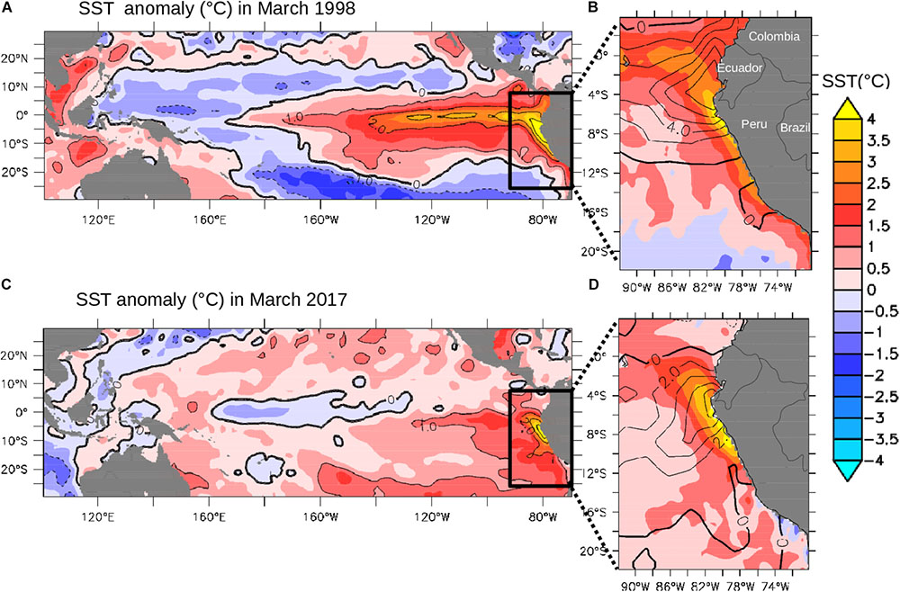
FIGURE 1. (A) SST anomaly (in °C) and (B) SST anomaly (in °C, color scale) and precipitation (in mm day^-1, contours) during the 1997–1998 El Niño in March 1998; (C,D) are same as (A,B) during the 2017 coastal El Niño in March 2017. Anomalies were computed with respect to the 1981–2016 climatology.

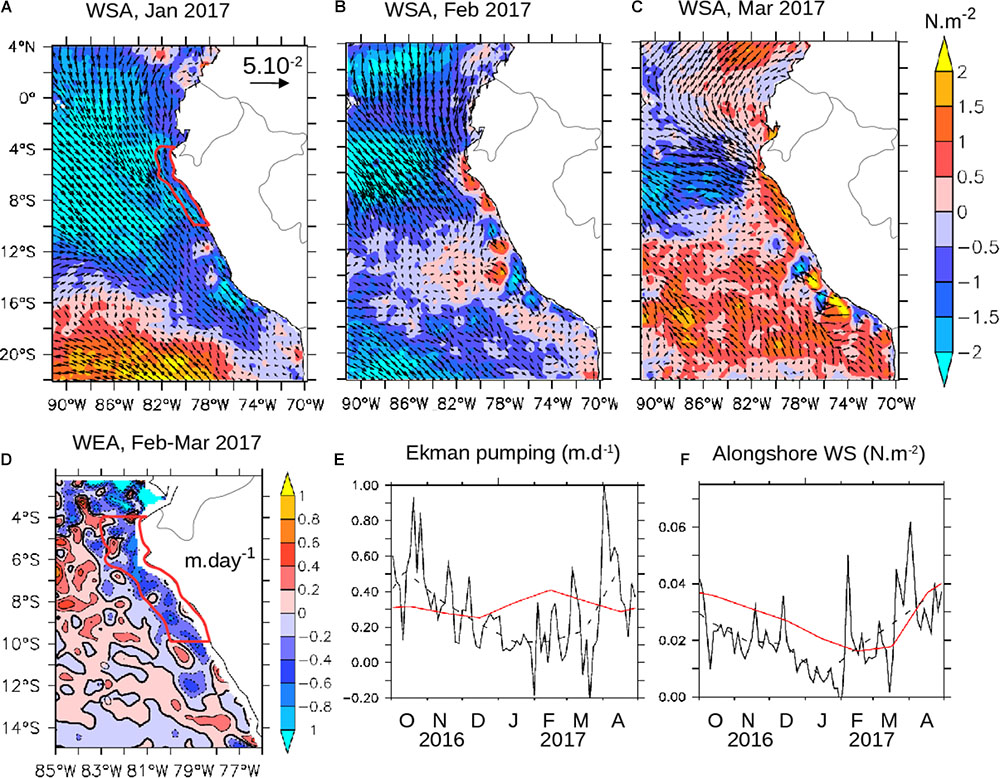
FIGURE 2. ASCAT monthly mean wind stress anomalies (in N m^-2) in 2017: (A) January, (B) February, (C) March. Anomalies were computed with respect to a climatology over 2013–2016. (D) Mean Ekman pumping velocity anomaly (in m day^-1, positive upward) in February-March 2017. (E) Ekman pumping velocity (in m day^-1, positive upward) in a coastal box (4–10°S, 0–200 km) from the coast, see red box in (D). (F) Alongshore wind stress in a coastal box (4–10°S, 0–100 km) from the coast, see red box in (A). The alongshore direction was the mean orientation of the coastline between 6°S and 10°S. Red and dashed lines mark climatological (over 2013–2016) and monthly mean values, respectively.

Strong coastal warming has occurred in other regions. The ’Ningaloo Niños’ (Feng et al., 2013) off the western coast of Australia are generated by cyclonic anomalies in the Mascarene subtropical anticyclone (Marshall et al., 2015). The wind relaxation reduces the ocean latent heat release, and the SST anomalies are then sustained by the poleward advection of warm water by the Leeuwin Current. Nevertheless, Ningaloo Niños are much more frequent than the coastal El Niños in the far-eastern Pacific, as the Mascarene subtropical high is often impacted by atmospheric teleconnections during La Niña (Marshall et al., 2015). A recent anomalous warming (the California “blob,” Peterson et al., 2015) was observed in the eastern North Pacific in the boreal winter of 2013–14, while El Niño conditions were neutral. The surface warming was triggered by an anomalously high-pressure system, which mitigated the wintertime cooling (Bond et al., 2015). The anomalously warm water was subsequently advected toward the northwestern coasts of the United States, generating major changes in the marine trophic chain and mild conditions over the continent.

In the present study, we investigate the regional forcings (e.g., wind anomalies, surface ocean currents, ocean-atmosphere feedbacks) and large-scale teleconnections (following Garreaud, 2018) that generated a strong surface ocean warming in the far-eastern Pacific in late summer 2017. The temporal evolution of the event is first characterized using satellite and in situ observations. The local oceanic and atmospheric drivers of the warming are then investigated using a regional ocean circulation model. Last, we study the teleconnections that initiated the wind relaxation at the origin of the surface warming using climate reanalysis data. In the following sections, we first describe the observations, followed by the model experiments and methodology (section Data and Methods). Results are presented in section “Results” and discussion and conclusions in section “Discussion and Conclusion.”

Data and Methods

Satellite Data

Several remotely sensed gridded products that were used for the analysis are as follows:

– The 1° × 1° daily NOAA Optimum Interpolation (OI) V2 sea surface temperature (SST) product for the period 1981–2017 was used¹. A description of the OI analysis, which merges satellite and in situ SST observations can be found in Reynolds et al. (2007). Note that this product is prone to be biased toward the climatology in the presence of stratocumulus cloud cover (Bretherton et al., 2010) in the Peru region.

– The gridded (1/4° × 1/4°) CMEMS (Copernicus Marine Environment Monitoring Service) daily sea level anomalies (SLA) were used. Data from all altimeter missions during the period 1993–2017 were merged to build a single product. It was downloaded on footnote².

– The daily surface winds and wind stress from the Advanced Scatterometer (ASCAT, 1/4° × 1/4°), the daily Quick Scatterometer (QuikSCAT, 1/2° × 1/2°), and weekly European Remote Sensing ERS wind stress (1° × 1°) were used. The gridded products were processed by CERSAT (2002a,b) and Bentamy and Fillon (2012) and downloaded from http://www.ifremer.fr/cersat.

– The gridded (2.5 × 2.5°) monthly precipitation product from the Global Precipitation Climatology Project (GPCP) was used. Data from rain gauge stations, satellites, and sounding observations were merged to estimate the monthly rainfall from 1979 to the present (Adler et al., 2003). The data was provided by the NOAA/OAR/ESRL Physical Sciences Division and downloaded from https://www.esrl.noaa.gov/psd/.

Climate Reanalysis

Monthly surface winds and precipitation from the NCEP/NCAR (hereafter NCEP; Kalnay et al., 1996), NCEP-DOE (hereafter NCEP2; Kanamitsu et al., 2002), and ERA-interim (hereafter ERAI; Dee et al., 2011) reanalysis were used to study teleconnections between surface winds in the eastern South Pacific and regions of atmospheric deep convection in the South Pacific in the period 1980–2017. Time correlation between the monthly precipitation fields and a monthly time series of meridional wind spatially averaged in a box located north-west of Peru (4°–10°S,90°–83°W) was computed for the month of January, when the wind relaxation occurred. The time period used to compute the correlations was 1980–2016.

In situ Observations

In situ temperature measurements were collected along cross-shore sections off Chicama (8°S) during monthly cruises performed by the Peruvian Institute of Sea Research (Instituto del Mar del Peru, IMARPE) on board R/V IMARPE V. The data were collected on March 27–28th, 2017, using a Sea Bird Electronics CTD profiler (type SBE 19 V2) each meter between the surface and 500 m depth. The water column was sampled at a distance of 5, 15, 30, 45, 60, 80, and 100 nautical miles (∼185 km) from the coast. A monthly climatology computed from IMARPE measurements during 1981–2010 (Dominguez et al., 2017) was substracted to the March 2017 data to obtain temperature anomalies.

Regional Modeling

The CROCO (Coastal and Regional Ocean Community model) was used to model ocean dynamics. CROCO is a new oceanic modeling system built upon ROMS_AGRIF and a new non-hydrostatic kernel (not used in this study). As the Regional Ocean Modeling System (ROMS), CROCO resolves the Primitive Equations, which are based on the Boussinesq approximation and hydrostatic vertical momentum balance. A third-order, upstream-biased advection scheme allows the generation of steep tracer and velocity gradients (Shchepetkin and McWilliams, 1998). For a complete description of the model numerical schemes the reader can refer to Shchepetkin and McWilliams (2005). The code used in this study is the CROCO v1.0 version, which is very similar to ROMS_AGRIF (Penven et al., 2006; Shchepetkin and McWilliams, 2009) in its version v3.1.

The model domain spans over the coasts of south Ecuador and Peru (from 5°N to 22°N) and from 92°W to 70°W. It is similar to the one used in Penven et al. (2005). The horizontal resolution is 1/9°, corresponding to ∼12 km. The bottom topography from ETOPO2 (Smith and Sandwell, 1997) is interpolated on the grid and smoothed in order to reduce potential error in the horizontal pressure gradient. The vertical grid has 32 sigma levels.

Several simulations of the 2017 warm event forced with contrasted forcings were compared in order to investigate the impact of different processes. Besides, the 1997–1998 El Niño event was simulated with the same model configuration and compared to the 2017 event. The different forcings and simulations are described as follows and summarized in Table 1.

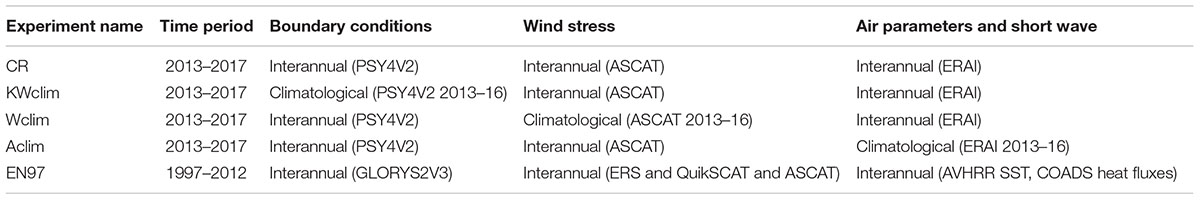
TABLE 1. Name and characteristics of the CROCO regional simulations.

Open Boundary Conditions (OBC)

Open boundary conditions (OBC) for physical variables (temperature, salinity, velocities, and sea-level) were treated using a so-called mixed passive/active scheme (Marchesiello et al., 2001). Barotropic velocities and sea level values were imposed following the conservation of characteristics (Blayo and Debreu, 2005). External OBC daily forcing from the Mercator-Ocean global reanalysis GLORYS2V3 at 1/4° (Lellouche et al., 2013; Masina et al., 2015) was used for the period January 1997-December 2012, and daily forcing from the Mercator-Ocean global analysis/forecast system PSY4V2 at 1/12° (Lellouche et al., 2018) was used for the period January 2013–March 2017. Altimeter data, in situ temperature, and salinity vertical profiles and satellite SST were jointly assimilated in GLORYS2V3 and PSY4V2. Both products are freely distributed by the Copernicus Marine Environment Monitoring Service (see text footnote²).

Atmospheric Forcing

ERAI daily net downward short-wave heat flux was used for insolation. Daily ASCAT wind speed, ERAI air temperature and humidity, and ROMS SST were used to compute latent and sensible heat flux online using a bulk parameterization (Liu et al., 1979) for the 2013–2017 period. Daily ASCAT wind stress was used to force the surface momentum fluxes, rather than the wind stress derived from the Liu et al. (1979) parameterization implemented in ROMS, because the latter was systematically weaker in the region of study. For the 1997–1998 period, climatological short-wave heat flux, net heat flux, and net freshwater flux (E-P) from COADS (Da Silva et al., 1994), and ERS (1997–1999) weekly wind stress were used. This simulation was resumed until 31 December 2012 using QuikSCAT (2000–2008) and ASCAT (2009–2017) daily wind stress. It should be noted that although differences between the two scatterometer winds have been evidenced (Bentamy et al., 2012), the transition from QuikSCAT to ASCAT in January 2009 did not have a noticeable impact on the modeled circulation in our region of interest. Bulk parameterizations were not used during 1997–2012, and SST was restored toward daily NOAA OI SST following Barnier et al. (1995). Note that this simulation (in particular the 1997–1998 time period) is only briefly used in the following to compare a few aspects of the strong 1997–1998 El Niño event with the 2017 coastal El Niño.

The atmospheric forcing fields, physical initial and OBC were interpolated onto the CROCO grid using MATLAB routines from the ROMSTOOLS pre-processing package (Penven et al., 2008).

Numerical Simulations

The following numerical experiments were performed (see Table 1):

– The EN97 simulation was run from 1 January 1997 to 31 December 2012 using the interannual atmospheric and OBC forcing described previously. Only the 1997–1998 period was analyzed in the present study. Initial conditions on 1 January 1997 were provided by a climatological ROMS simulation performed in a previous work (Echevin et al., 2014), thus no spin up was needed for EN97.

– The control run (CR) forced by daily interannual atmospheric forcing and OBC was run from 1 January 2013 to 30 March 2017. Initial conditions on 1 January 2013 were provided by EN97.

– The Wclim simulation forced by ASCAT monthly climatological winds and wind stress (the climatology was computed over the 2013–2016 period), daily interannual shortwave, precipitation, air temperature and humidity, and daily interannual OBC, was run from 1 January 2016 to 30 March 2017. The comparison of Wclim with CR allowed to investigate the effect of the wind relaxation in late 2016 and early summer 2017. Initial conditions on 1 January 2016 were provided by CR.

– The KWclim simulation forced by daily interannual atmospheric forcing (as in CR) and monthly climatological OBC was run from 1 January 2017 to 30 March 2017. The monthly climatological OBC was computed for January, February, and March for the period 2013–2016. Note that coastal trapped waves were present in 2013–2016 but the monthly climatology reduced their intensity drastically (see section Sea Level Anomalies and Horizontal Circulation). The comparison of KWclim with CR allowed to investigate the effect of the equatorially forced downwelling Kelvin waves on the anomalous warming during summer 2017. Initial conditions on 1 January 2017 were provided by CR.

– The Aclim simulation forced by climatological heat fluxes (short wave radiation, air temperature, and humidity), daily interannual wind and wind stress, and daily interannual OBC, was run from 1 January 2017 until 30 March 2017. Initial conditions on 1 January 2017 were similar to those for KWclim.

Heat Budget in the Mixed Layer

A heat budget was performed to study the processes responsible for the mixed layer temperature evolution. The temperature evolution equation is averaged for each time step in the model mixed layer, leading to different terms corresponding to the rate of change of SST, lateral and vertical advection of heat, and heat exchange through the base of the mixed layer by vertical mixing (defined here as the sum of entrainment/detrainment and vertical diffusion at the mixed layer base; Jullien et al., 2012). The mixed layer depth is equal to the boundary layer depth which is determined by comparing a bulk Richardson number to a critical value (KPP parameterization; Large et al., 1994).

Results

Atmospheric and Oceanic Conditions During Summer 2017

Wind stress conditions were unusually weak off Peru since the last quarter of 2016 and particularly in January 2017. During this month, poleward anomalies reaching ∼0.2 N m^-2 nearshore and offshore were encountered, particularly in the north of Peru (Figure 2A). In February, the wind stress remained very weak offshore in the north of Peru, whereas it started to increase nearshore along the northern coast (4°S–10°S) and further south (12°S, Figure 2B). In the second half of March a strong alongshore upwelling-favorable wind stress anomaly developed over most of the central shelf of Peru (5°S–13°S). A poleward wind stress anomaly off the coast of Ecuador generated a strong convergence near (82°W, 4–6°S) (Figure 2C). The nearshore wind stress increase and the offshore wind stress relaxation off northern Peru generated an intense wind stress curl anomaly and an associated negative Ekman pumping anomaly (Figure 2D). Ekman pumping was much weaker than the climatology between mid-December and the end of March (Figure 2E). It reached negative values during short time periods of a few days at the end of January and mid-March, generating a local downwelling. The occurrence of such downwelling driven by Ekman pumping has been previously observed off southern Peru (15°S) during the 1997–1998 El Niño event (Halpern, 2002).

We now investigate the potential role of large-scale oceanic conditions in the nearshore warming. A Hovmöller diagram of along-equator (in the Equatorial Pacific between 140°E and 80°W) and along-coast (between 0°Sand 22°S, e.g., see Figure 2 in Colas et al., 2008) altimetric SLA (Figure 3) shows positive anomalies propagating along the equator as downwelling equatorial Kelvin waves and along the coast as coastally trapped waves during the summer of 2017. Nevertheless, these waves were relatively weak compared with those propagating during summer 2016 in the midst of the 2015–2016 El Niño and did not generate El Niño conditions in the central Pacific (Figure 1C). Nevertheless, such positive SLA are generally associated with a deepening of the nearshore thermocline along the coast of Peru (e.g., Espinoza-Morriberón et al., 2017), and thus may have strengthened the surface warming initiated by the wind relaxation.

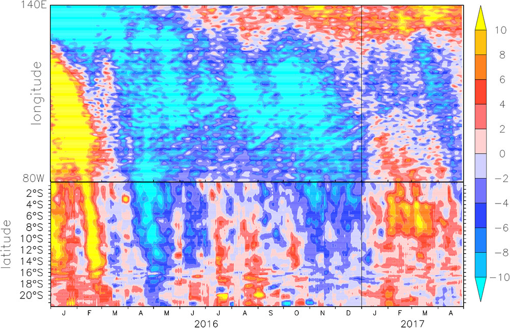
FIGURE 3. Hovmöller of altimetric sea level anomaly (in cm) along the equator (140°E–80°W) and along the coast of Peru (0–22°S). The sea level anomalies were computed using the 1/4° × 1/4° gridded product, such that for each latitude, the sea level observations were averaged between the coast and 50 km offshore. The anomalies were computed with respect to a 2013–2016 climatology.

Evolution of the SST and Vertical Temperature Structure

The SST anomalous patterns changed over the course of austral summer 2017. In January, the observed mean temperature near the northern coast was slightly colder than the climatology, with weak negative anomalies between -1 and 0°C (Figure 4A). There was a buildup of coastal positive anomalies during the following months, reaching a maximum of 2–3°C in February (Figure 4B) and more than 5°C in March (Figure 4C). The model was able to reproduce the January nearshore negative anomaly mainly off the south part of the shelf (Figure 4D). The model coastal SST anomalies reached a maximum of 4 and 5°C in February (Figure 4E) and March (Figure 4F), respectively. However, the spatial extension and intensity of the anomalous warming were slightly reduced in the model when compared to the observations.

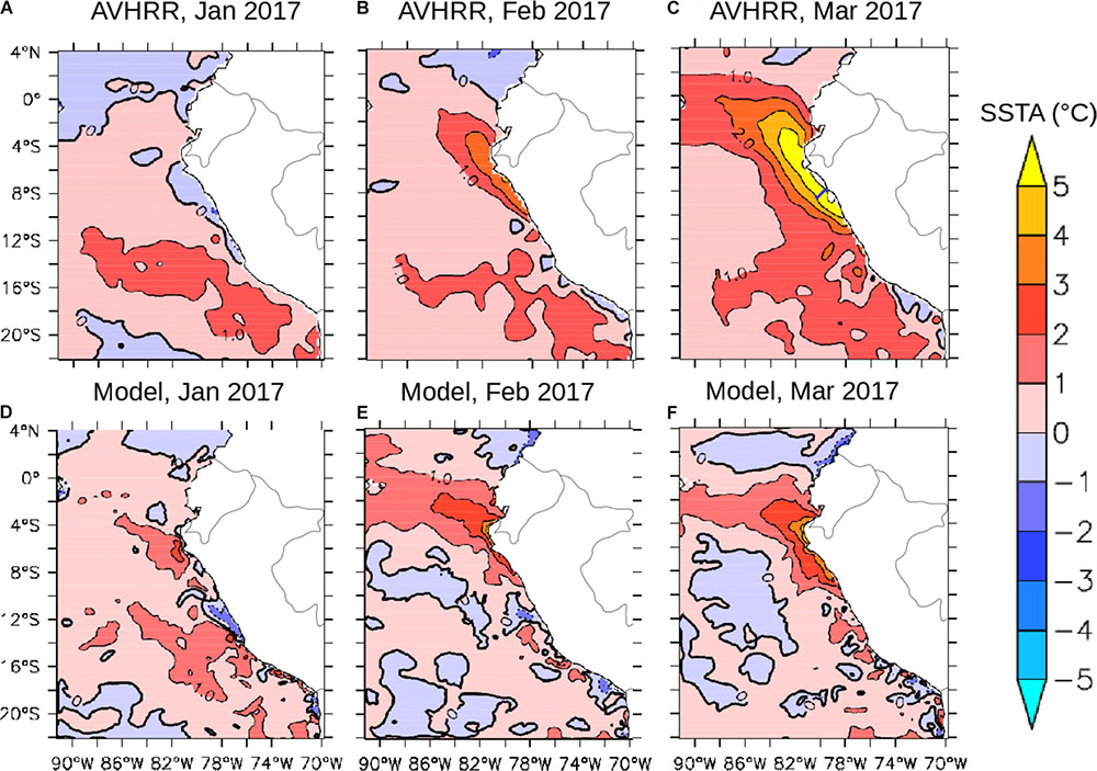
FIGURE 4. SST anomalies in (A,D) January, (B,E) February, and (C,F) March 2017 from SST observations (top) and model output (bottom). Anomalies were computed with respect to 2013–2016 climatology. The blue line in (C) indicates the location of the Chicama section.

The vertical structure of the temperature field in late March 2017 is examined using IMARPE in situ data collected along a cross-shore section near 8°S. On 27–28th March, the isotherms sloped upward toward the coast, indicative of coastal upwelling (Figure 5A), which was consistent with the enhanced alongshore wind stress signal (Figure 2F). The 15°C isotherm sloped downward toward the shore, thereby marking the presence of the poleward undercurrent. The modeled temperature section displays comparable patterns, such as upwelling in the surface layer (Figure 5B). The 15°C isotherm depth was relatively realistic in the model, whereas the thermocline was slightly shallower than in the observations.

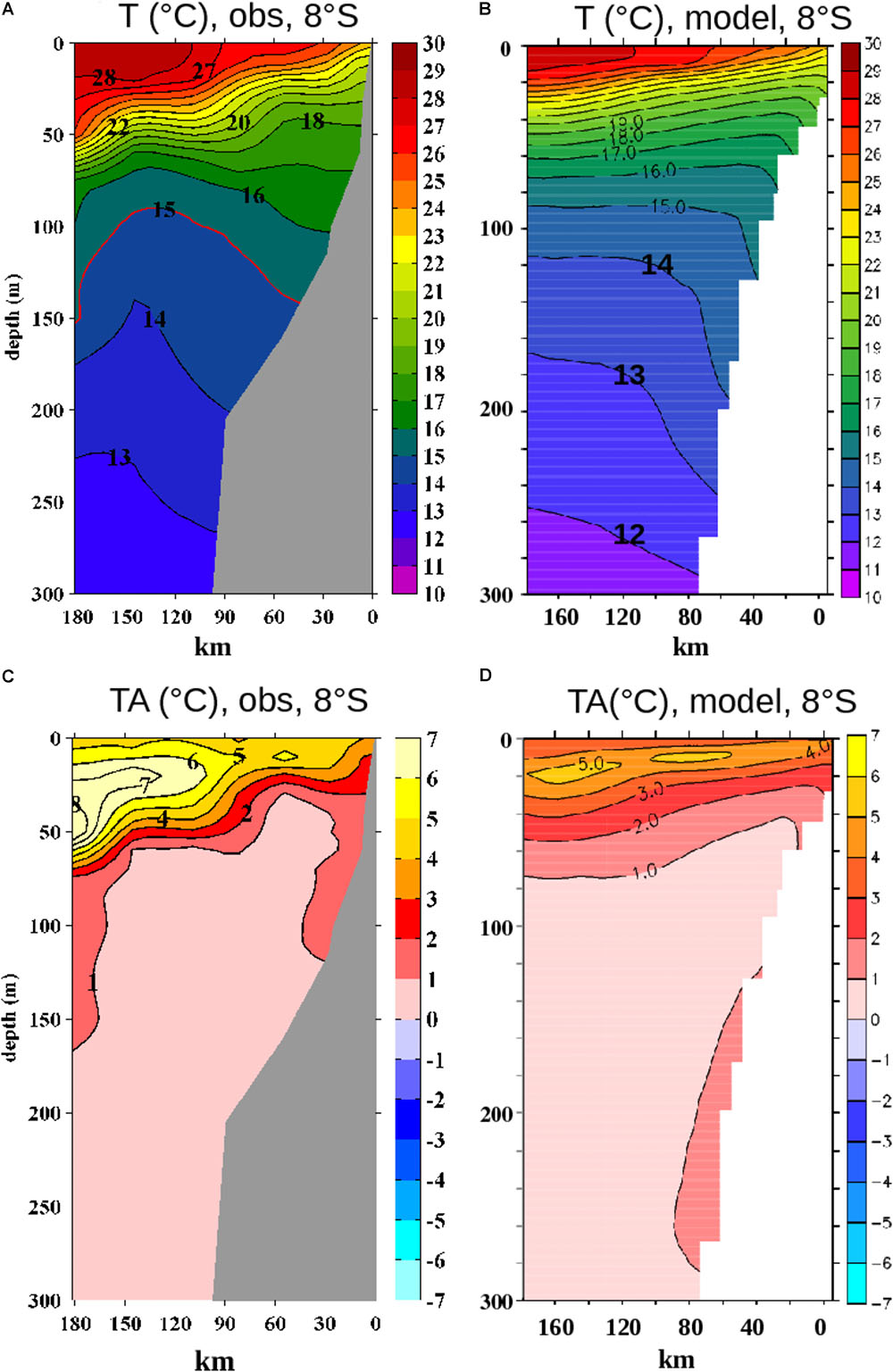
FIGURE 5. Cross-shore vertical sections of temperature (A,B) absolute values and (C,D) anomalies (in °C) in March 2017 off the northern Peru shelf (Chicama, 8°S). The section’s location is indicated in Figure 4C. Observed anomalies (c) were computed with respect to a climatology of IMARPE data for the period 1981–2010, while modeled anomalies were computed with respect to a model climatology for 2013–2016.

In situ temperature positive anomalies larger than +2°C were found above ∼60 m depth offshore and above ∼40 m near the coast (Figure 5C). The strongest anomalies (+7–8°C) were encountered offshore at ∼20 m depth, while the highest nearshore anomalies (∼ + 4°C) were found at the surface. Modeled positive anomalies larger than + 2°C were found above ∼50 m depth offshore and above ∼30 m depth near the coast (Figure 5D). The maximum anomalies reached +4°C near ∼20–30 m depth and were weaker than the observed ones. In conclusion, the model was able to represent the surface and subsurface thermal anomalies with a fair degree of realism.

Sea Level Anomalies and Horizontal Circulation

The spatial structure of SLA during the warm event sheds light on the surface geostrophic anomalous circulation. The observed sea level patterns did not display notable anomalies in January 2017 (Figure 6A). A large-scale positive SLA structure, with maximum values of ∼9 cm (near 3–5°S, 82–81°W), appeared in February and March (Figures 6B,C). It created a steep sea level slope and an intense onshore, south-eastward geostrophic current. The latter transported relatively warm offshore waters toward the coast near 10°S, and reduced the coastal divergence and offshore transport of relatively cold upwelled waters, thus enhancing the coastal warming in the southern part of the shelf. Comparable SLA structures were simulated by the model, differing slightly in the shape of the large-scale anomalous patterns (Figures 6B,C).

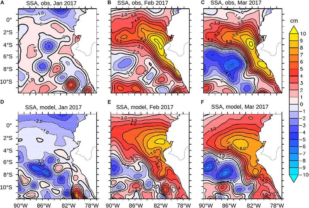
FIGURE 6. Sea level anomaly (in cm) in (A,D) January; (B,E) February; (C,F) March 2017, from satellite observations (top) and model (bottom). Anomalies were computed with respect to the 2013–2016 climatology.

The strong sea level rise was associated with a significant thermocline deepening in the model (Figure 7). The depth of the 20°C isotherm (hereafter D20, used here as a thermocline depth proxy) was relatively shallow (∼20 m) until late January 2017, much shallower than during El Niño events in January 1998 (∼120 m) or in January 2015 (∼ 50 m). D20 increased in February and March 2017, reaching approximately the same depth (∼30–35 m) as in March 2016. However, the thermocline remained much shallower than in March 1998 (∼ 60 m) during the extreme 1997–1998 El Niño event, showing that the 2017 warming was confined to a relatively shallow layer.

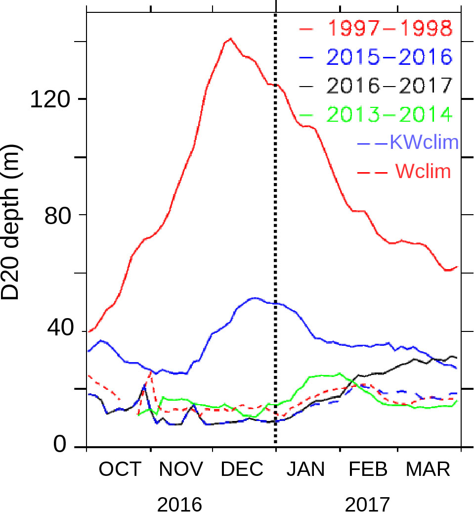
FIGURE 7. Time evolution of the depth of the 20°C isotherm (D20, in meters) between October (year–1) and March (year+1) for different time periods (see labels). D20 was averaged in a coastal box between 4°S and 10°S and within 200 km from the coast.

Heat Fluxes and Mixed Layer Heat Budget During Summer 2017

We now characterize the air-sea heat fluxes during the warm event. ERAI shortwave flux anomalies were weak in January (Figure 8A) and negative off northern Peru in February (Figure 8B) and March (Figure 8C), likely due to an increased cloud cover. Due to the wind relaxation in January (Figure 2), the surface ocean was less cooled than under climatological conditions by the latent heat release (Figure 8D; Garreaud, 2018). However, the latent heat flux anomalies turned negative due to the nearshore wind increase off northern Peru in February (Figure 8E) and March (Figure 8F). Consequently, the net heat flux anomalies were negative near the northern coast (Figures 8G–I), indicating that less heat than under climatological conditions was transferred from the atmosphere to the ocean during the coastal warming.

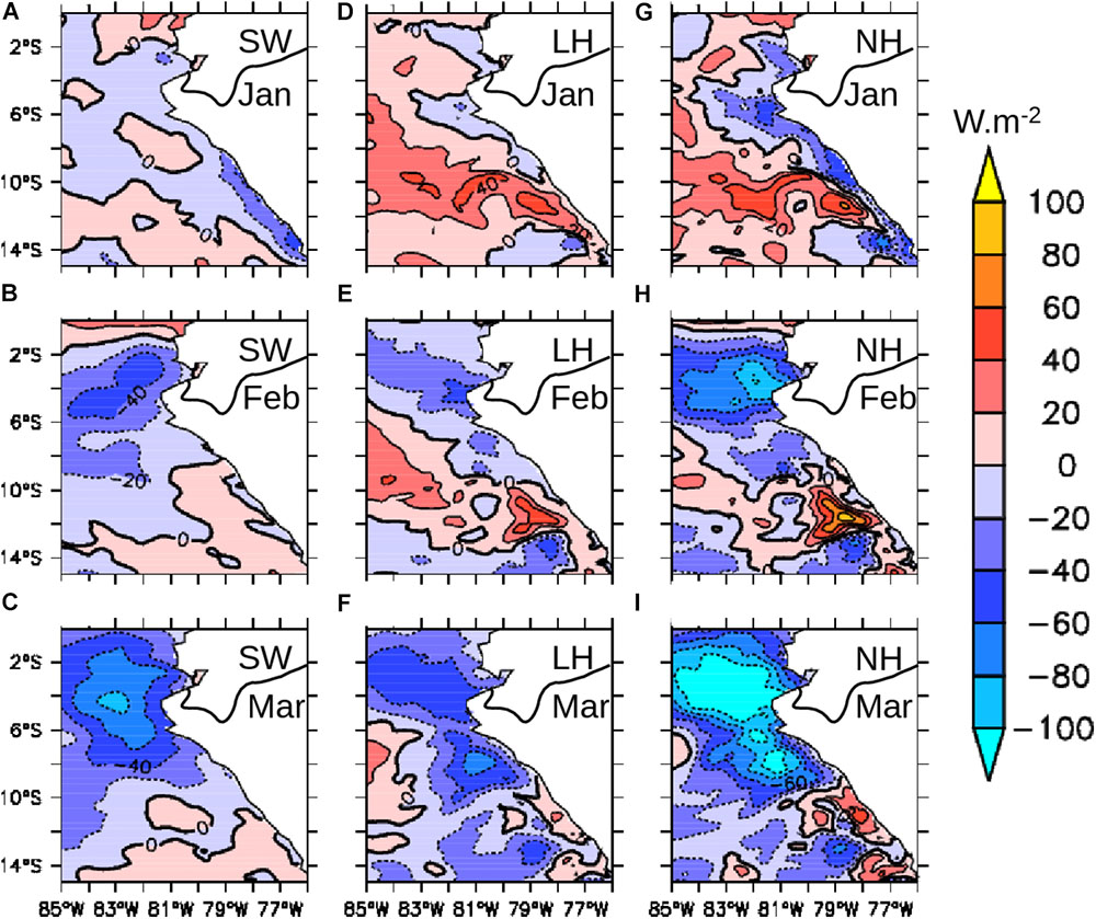
FIGURE 8. Monthly heat flux anomalies (in W m^-2, positive downward) in January, February, and March 2017: (A–C) short wave heat flux anomaly (SW); (D–F) latent heat flux anomaly (LH); and (G–I) net heat flux anomaly (NH). Positive fluxes indicate an input of heat into the ocean. Anomalies were computed with respect to the 2013–2016 model climatology.

The drivers of the mixed layer SST evolution were investigated using the mixed layer heat budget terms (see section Data and Methods). Anomalies of the temperature rates in January-March 2017 represent the growth of the temperature anomaly in the mixed layer. The SST anomaly increased mainly in January (Figure 9A) and February (Figure 9B), and began to decrease in March (Figure 9C). The January warming was driven both by the atmospheric forcing (Figure 9D) and advective processes (Figure 9J). As the mixed layer was shallower (by ∼6 m, Figure 9A) than its climatological value, the deposition of heat in an abnormally shallow mixed layer allowed the latter to warm, in spite of the negative net heat flux anomalies (Figure 8G). This heating was partly compensated by entrainment. As the shallow mixed layer deepened during January (not shown), entrainment of cool water into the mixed layer resulted in an anomalously strong cooling (Figure 9G). More importantly, coastal upwelling was strongly reduced owing to the weak alongshore wind stress (Figure 2). Thus, less cool subsurface water was advected through the mixed layer base (Figure 9J), which amplified the surface warming.

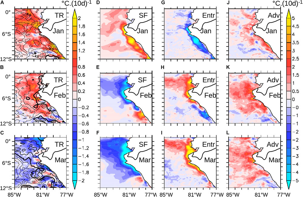
FIGURE 9. Heat budget in the surface mixed layer. (A–C) Mixed layer temperature rate of change (TR, in °C/10 days, color scale) and mixed layer depth (in meters). The contour interval is 2 m, dashed (full) lines mark negative (positive) values. (D–F) Surface forcing (SF, in °C/10 days). (G–I) Entrainment (Entr, in °C/10 days). (J–L) Advection (horizontal + vertical, Adv, in °C/10 days). Top, middle, and bottom rows correspond to January, February, and March 2017, respectively. Anomalies were computed with respect to the 2013–2016 climatology.

When the wind became anomalously strong near the northern coast in February and March, the mixed layer deepened nearshore (Figures 9B,C). In contrast to January, the cooling of the mixed layer in February and March (Figures 9E,F) was partly compensated by entrainment (Figures 9H,I). Indeed, anomalously warm subsurface water (due to the deepening of the thermocline driven by anomalous Ekman pumping and downwelling coastal waves, Figure 7) was entrained into the mixed layer. Advection also contributed to the warming (Figures 9K,L) due to the shoreward flow of warm surface waters (Figure 6) and the reduced Ekman pumping (Figures 2D,E). Note that the enhanced wind-driven coastal upwelling in March (Figure 2) slightly mitigated the nearshore warming between 6° and 8°S (Figures 9C,L).

Relative Impacts of the Wind and Equatorial Oceanic Forcing

Overall, the atmospheric forcing played a major role in the mixed layer warming, first by forcing a decrease of the coastal upwelling at the beginning of the event, then by creating a strong wind stress curl (Figures 2D,E) which deepened the thermocline (Figure 7). However, the passage of downwelling coastal trapped waves may also have impacted the warming by deepening the thermocline near the coast. In the following paragraphs, we analyze the model experiments performed with modified forcings (see section Data and Methods) to evaluate the relative contribution of each forcing to the surface warming.

Figure 10 displays the nearshore SST evolution off northern Peru in the different model experiments and observations. The CR-modeled SST was overestimated by ∼2°C in January and underestimated by ∼1–2°C in March 2017. The CR SST also displayed oscillations, peaking in late January, late February, and mid-March 2017. The KWclim SST, in which the impact of downwelling coastal waves was suppressed, was similar to the CR SST until the beginning of February. Then, it became weaker than in the CR, the difference reaching ∼2°C in late February-March. This indicates that the February-March remotely forced waves induced a warming of ∼ + 2°C in the nearshore region.

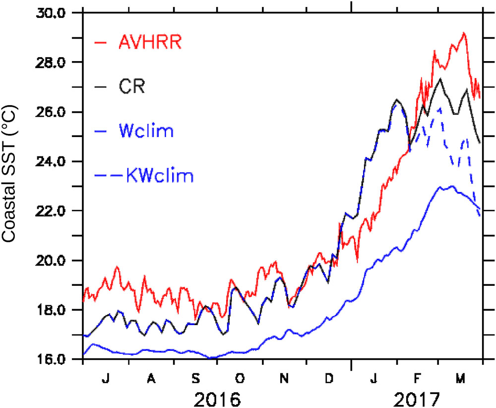
FIGURE 10. Time evolution of the SST averaged in a coastal box (4–10°S, 0–100 km from the coast) for AVHRR observations (red line), CR (black line), Wclim (blue line), and KWclim (dashed blue line).

Nevertheless, the effect of the wind anomalies was much stronger than that of the coastal waves, as shown by the Wclim SST. Nearshore surface winds were relatively weak during austral spring 2016 (Figure 2F), which led to an SST difference of ∼ + 1–2°C between CR and Wclim during winter and spring 2016. The SST difference between CR and Wclim increased strongly in January 2017, reaching ∼ + 6.5°C at the end of the month. Then a wind-driven upwelling event (Figure 2F) cooled the surface layer by ∼2°C in CR. The SST difference between CR and Wclim remained around ∼3–4°C until the end of March 2017. The absence of SST oscillations in Wclim during January-March 2017, in contrast with CR and KWclim, was likely due to the absence of 10–25 days of wind variability (Dewitte et al., 2011) in the climatological wind forcing.

The spatial patterns forced by the weak winds and downwelling coastal waves during summer 2017 were investigated by computing the anomalies between the CR and modified forcing experiments SST fields. The spatial structure of the CR-Wclim SST anomaly in March 2017 (Figure 11A) resembles the CR SST anomaly with respect to the climatology (Figure 4F), suggesting that the anomalous wind stress forcing was the main driver of the surface warming in the north (2°S–6°S) of the region of study. Nevertheless, the coastal waves also impacted the nearshore temperature near 7–8°S. The CR-KWclim SST anomaly was confined to the coastal zone and weaker (∼ + 4°C, Figure 11B) than the more extended and stronger (up to ∼ + 5°C, Figure 11A) anomaly associated with the wind anomalies. In agreement with the previous results, both the wind anomalies and the coastal waves contributed to the nearshore thermocline deepening, in approximately equal proportions (∼18 cm, Figure 7). Besides, the Aclim simulation (see section Numerical Simulations and Table 1) did not produce any noticeable differences with respect to the CR (Figures not shown), confirming that insolation anomalies (Figure 8) had a negligible impact on the warming.

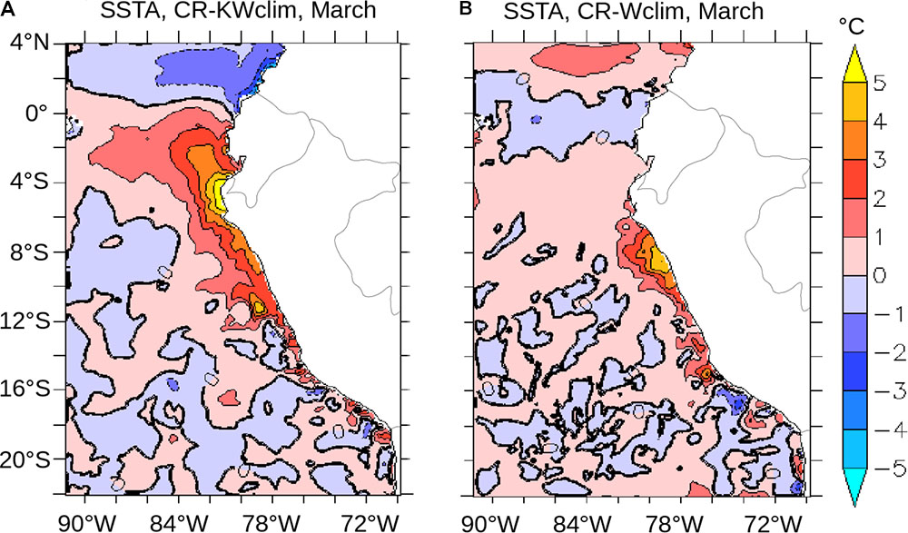
FIGURE 11. March 2017 SST difference (in °C) between the control run (CR) and sensitivity runs: (A) CR-Wclim and (B) CR-KWclim.

Large-Scale Forcing of the January Wind Relaxation

The large-scale dynamical mechanisms driving the January wind relaxation are now investigated, in an attempt to complement the findings of Garreaud (2018). Using NCEP, NCEP2, and ERAI reanalysis over the period 1980–2016, we computed correlations between monthly precipitation (a proxy of deep convection in the atmosphere) over the tropical and south Pacific Ocean and an index of meridional wind intensity in the far- eastern Pacific (see section Climate Reanalysis) during January (Figure 12). Relatively high correlations (>0.5) were found over north-eastern Amazonia, indicating a plausible teleconnection between enhanced deep convection in this region and surface wind relaxation in the far-eastern Pacific. Note that surface wind relaxation was also associated with a reduction of deep convection in the western and central Pacific.

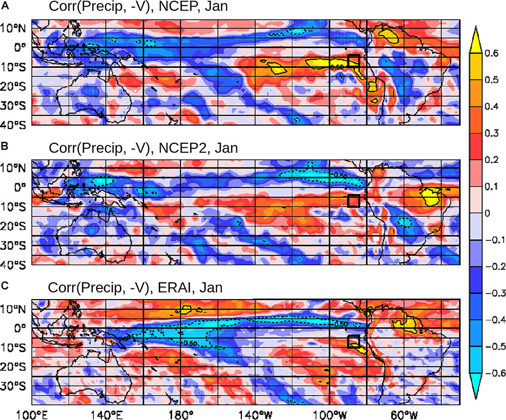
FIGURE 12. Correlation between South and Equatorial Pacific monthly precipitation and meridional wind (positive when oriented poleward, averaged in black square) in the far-eastern Pacific in January. The correlations were computed from three different reanalyses products: (A) NCEP, (B) NCEP2, and (C) ERAI. Monthly anomalies were computed over 1979–2016. Full and dashed contours mark correlations of 0.5 and –0.5, respectively.

We now investigate whether anomalous deep convection occurred at these locations in January 2017. Observed and reanalysis precipitations were anomalously intense over central Australia (Figure 13) during this time period, which were in agreement with the negative outgoing long wave anomalies evidenced by Garreaud (2018). Precipitations were also anomalously intense over eastern Amazonia. This suggests that the surface wind relaxation may have been forced by atmospheric teleconnections between the western and far-eastern Pacific (Takahashi and Martínez, 2017; Garreaud, 2018) but enhanced convection (i.e., release of heat of the upper atmosphere) over the Amazonia may have impacted the South Pacific Anticyclone (SPA) (Miyasaka and Nakamura, 2010).

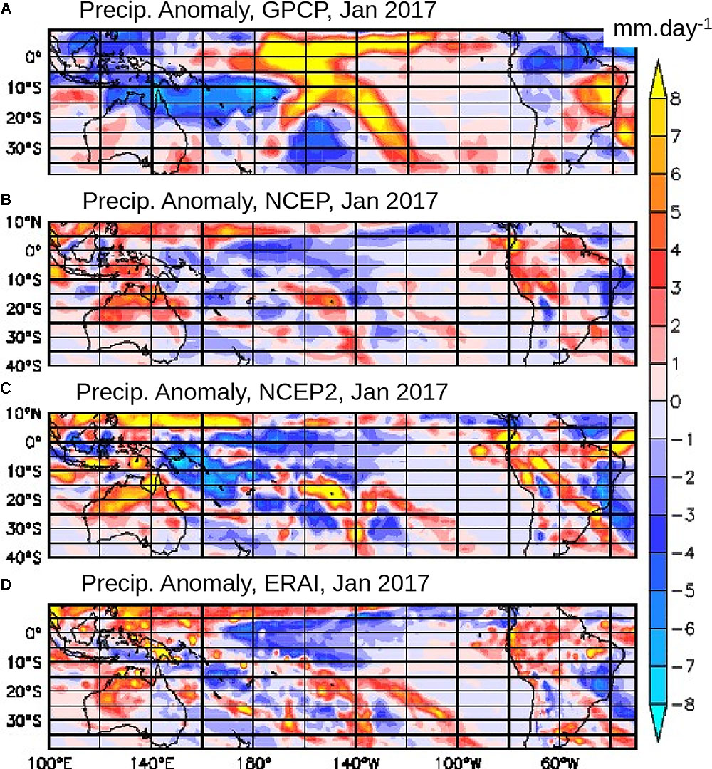
FIGURE 13. Mean precipitation anomaly (in mm day^-1) in January 2017 from: (A) GPCP, (B) NCEP, (C) NCEP2, and (D) ERAI. Monthly anomalies were computed over the period 1979–2016.

Discussion and Conclusion

An exceptional warming of the surface ocean took place off the coast of northern Peru and Ecuador in late summer 2017, producing catastrophic flooding and landslides. Its duration was much shorter than previous Eastern Pacific El Niño events but SST anomalies and precipitations were nevertheless very intense. As there were no signs of anomalously high temperatures in the equatorial Pacific, the intense coastal warming and its consequences were not anticipated by the local governmental agencies or by the scientific community (Ramirez and Briones, 2017). In the present study, in agreement with Garreaud (2018), we found that the initial warming was mainly associated with a regional decrease of the winds in the far-eastern Pacific. Offshore and nearshore winds were weak in late 2016, and continued to drop until the end of January 2017, which shut down the wind-driven coastal upwelling. In February, nearshore winds began to increase while the offshore winds remained weak, resulting in a strong wind stress curl which deepened the thermocline and enhanced the warming through negative Ekman pumping. The local thermocline deepening was associated with a sea level rise off the coasts and a shoreward geostrophic current anomaly intensifying the coastal warming. Similar onshore geostrophic currents were evidenced in simulations of El Niño events (Colas et al., 2008; Espinoza-Morriberón et al., 2017).

The strong wind stress curl anomaly, caused by the offshore relaxation and nearshore wind intensification in February and March 2017, played a major role in the warming. A comparable wind stress curl anomaly developed during the 1997–1998 El Niño off southern Peru near Pisco (15°S), enhancing the downwelling primarily driven by the very intense downwelling coastal trapped waves (Halpern, 2002). The dynamical processes responsible for the 1997–1998 nearshore wind increase were recently analyzed by Chamorro et al. (2018). Using a regional atmospheric model, the authors showed that the increase of nearshore wind was driven by the SST alongshore gradient, associated with the accumulation of warm waters along the northern shores of Peru. We believe that a similar sequence of events may have taken place during the summer of 2017, albeit with a different initialization process than during classical El Niño events. During the 2017 coastal El Niño, the January wind relaxation reduced the coastal upwelling and generated a positive SST anomaly off northern Peru and Ecuador (Figure 4), thereby creating an alongshore temperature gradient (Figure 14). After reaching its weakest value in late January, the coastal wind increased in phase with the SST gradient and recovered climatological values by mid-February. Subsequently both the SST gradient and the coastal wind reached a plateau between mid-February and mid-March. Note that the strong wind increase in late March cannot be only explained by this paradigm, as a large-scale wind intensification also took place (Figure 2C). During February and March, the Ekman pumping negative anomaly associated with the wind stress curl (Figure 2E) may have deepened the thermocline, and thus the cooling due to enhanced upwelling at the coast may have been mitigated by the upward flux of anomalously warm source waters. The atmospheric response to the SST gradient, described by Chamorro et al. (2018) for the 1997–1998 El Niño, may thus feedback positively on the warming initiated in January. The ocean-atmosphere coupled processes occurring during this event would need to be more fully investigated using a regional coupled ocean-atmosphere model (Oerder et al., 2016, 2018).

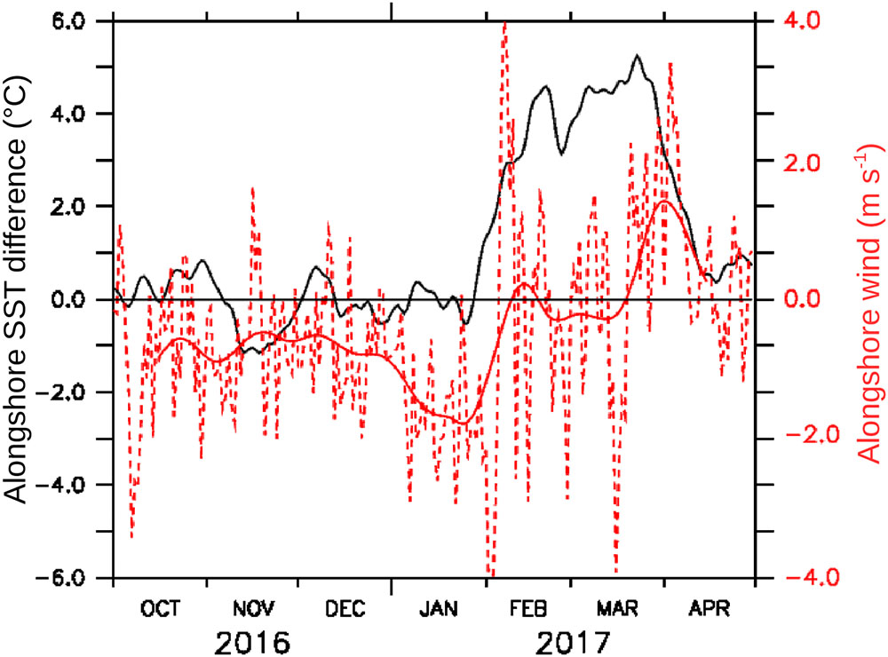
FIGURE 14. Alongshore SST difference (in °C, black line) and alongshore wind anomaly (in m s^-1, red line). The SST difference was computed as the difference between the SST averaged in a northern coastal box (6–10°S, 0–100 km from the coast) and a southern coastal box (10–16°S, 0–100 km from the coast). The alongshore direction was the mean orientation of the coastline between 6°S and 14°S.

Our regional model represented the spatial patterns of the SST anomaly relatively well but with a weaker intensity with respect to SST observations (Figure 4). This could be partly attributed to biases in the atmospheric heat fluxes, in particular to the ill-representation of the eastern Pacific low cloud deck in atmospheric models (Wyant et al., 2010). Moreover, the absence of SST decrease in the data (Figure 10) during the late January coastal upwelling event is puzzling. Although cloud cover was not anomalously strong during this period (Figure not shown), gaps in the satellite data could explain this discrepancy. Indeed, missing data are filled by in situ and climatological observations to produce a cloud-free SST product (Reynolds et al., 2007). An alternative explanation could be that the upwelling of anomalously warm source waters in early February did not produce an SST decrease. This may not be well represented by the model as the subsurface source water temperature anomaly may have been underestimated (Figures 6C,D).

The large-scale mechanisms triggering coastal El Niños, and the 2017 event, are still not well known due to their scarcity. During the 1925 coastal El Niño, which bears similarities with the 2017 event, the northeasterly flow related with the Panama gap jet and the southeasterly trades associated with the SPA were not particularly anomalous (Takahashi and Martínez, 2017). To explain the low coastal winds off Peru, these authors proposed that a reduction of deep convection in the western-central Pacific and of zonal air moisture flow in the tropical troposphere may have displaced the ITCZ southward, enhancing precipitation along the northern Peruvian Andes (Sulca et al., 2018). Studying the 2017 event, Garreaud (2018) evidenced a teleconnection between the western and the far-eastern Pacific as a triggering mechanism. Using the NCEP2 reanalysis, he found that deep convection over central Australia in January 2017 triggered Rossby wave trains extending across the South Pacific (Mo and Higgins, 1998), which modified the tropospheric westerly flow impinging the subtropical Andes. The poleward shift of the flow modified subsidence in the SPA and reduced the southeasterlies. Note that according to our results, none of the three reanalyses produced a positive correlation pattern over central Australia (Figure 12). This suggests that Garreaud’s (2018) proposed teleconnection between the latter and the far-eastern Pacific by means of atmospheric Rossby waves is not a common feature in any of the reanalyses. Using the NCEP reanalysis over the period 1979–2001, Grotjahn (2004) evidenced a distinct teleconnection. He showed that enhanced deep convection (i.e., more precipitation) over eastern Amazonia coordinated with reduced deep convection (i.e., less precipitation) in the western tropical Pacific during austral spring-summer could impact the tropical side of the SPA, reducing surface winds. Forcing of the summertime SPA by the deep convective heating over the Amazonia has been evidenced in model experiments (Miyasaka and Nakamura, 2010). This teleconnection evidenced in several reanalysis products (Figure 12) may have played a role in the triggering of the wind relaxation which initiated the coastal warming. However, a dedicated and more thorough study would be necessary to better understand the atmospheric large-scale mechanisms initiating coastal El Niño events. It is beyond the scope of the present work and will be addressed in a future study.

Author Contributions

VE proposed the original idea of the study, produced most of the material, and wrote the manuscript. FC, DE-M, and DG discussed the results and corrected the manuscript. TA processed the in situ data. LV participated to the in situ data collection.

Funding

This work was partly supported by the French national program LEFE/INSU (project CIENPERU) and by the LMI DISCOH project. It is a contribution to the cooperative agreement between IMARPE and the Institut de Recherche pour le Développement (IRD).

Conflict of Interest Statement

The authors declare that the research was conducted in the absence of any commercial or financial relationships that could be construed as a potential conflict of interest.

Acknowledgments

We thank the IMARPE R/V crew in charge of the cruise off northern Peru during March 2017. Model simulations were performed on the Ada supercomputer at IDRIS (project x2016011140). Atmospheric reanalysis data was downloaded on the Ciclad IPSL server. Global ocean model outputs and sea level maps were provided from the Copernicus Marine Environment Monitoring Service (CMEMS). Francis Codron (LOCEAN) is acknowledged for fruitful discussion.

Footnotes

1. ^https://www.esrl.noaa.gov
2. ^http://marine.copernicus.eu/

References

Adler, R. F., Huffman, G. J., Chang, A., Ferraro, R., Xie, P., and Janowiak, J. (2003). The version 2 Global Precipitation Climatology Project (GPCP) monthly precipitation analysis (1979-present). Hydrometeor. J. 4, 1147–1167. doi: 10.1175/1525-7541(2003)004<1147:TVGPCP>2.0.CO;2
Barber, R. T., and Chavez, F. P. (1983). Biological consequences of el nino. Science 222, 1203–1210. doi: 10.1126/science.222.4629.1203
Barnier, B., Siefridt, L., and Marchesiello, P. (1995). Thermal forcing for a global ocean circulation model using a three-year climatology of ECMWF analyses. J. Mar. Syst. 6, 363–380. doi: 10.1016/0924-7963(94)00034-9
Bentamy, A., and Fillon, D. C. (2012). Gridded surface wind fields from Metop/ASCAT measurements. Int. J. Remote Sens. 33, 1729–1754. doi: 10.1080/01431161.2011.600348
Bentamy, A., Grodsky, S. A., Carton, J. A., Croizé-Fillon, D., and Chapron, B. (2012). Matching ASCAT and QuikSCAT winds. Geophys. J. Res. 117:C02011. doi: 10.1029/2011JC007479
Bjerknes, J. (1969). Atmospheric teleconnections from the equatorial Pacific. Mon. Weather Rev. 97, 163–172. doi: 10.1175/1520-0493(1969)097<0163:ATFTEP>2.3.CO;2
Blayo, E., and Debreu, L. (2005). Revisiting open boundary conditions from the point of view of characteristic variables. Ocean Model. 9, 231–252. doi: 10.1016/j.ocemod.2004.07.001
Bond, N. A., Cronin, M. F., Freeland, H., and Mantua, N. (2015). Causes and impacts of the 2014 warm anomaly in the NE Pacific. Geophys. Res. Lett. 42, 3414–3420. doi: 10.1002/2015GL063306
Bretherton, C. S., Wood, R., George, R. C., Leon, D., Allen, G., and Zheng, X. (2010). Southeast Pacific stratocumulus clouds, precipitation and boundary layer structure sampled along 20 S during VOCALS-REx. Atmos. Chem. Phys. 10, 10639–10654. doi: 10.5194/acp-10-10639-2010
Carranza, L. (1891). Contra-corriente marítima observada en Paita y Pacasmayo. Boletín Sociedad Geográfica Lima 9, 344–346.
Chamorro, A., Echevin, V., Colas, F., Oerder, V., Tam, J., and Quispe-Ccalluari, C. (2018). Mechanisms of the intensification of the upwelling-favorable winds during El Niño 1997–1998 in the Peruvian upwelling system.Clim. Dyn. 1–17. doi: 10.1007/s00382-018-4106-6
Colas, F., Capet, X., McWilliams, J. C., and Shchepetkin, A. (2008). 1997–1998 El Niño off Peru: a numerical study. Prog. Oceanogr. 79, 138–155. doi: 10.1016/j.pocean.2008.10.015
Da Silva, A. M., Young, C. C., and Levitus, S. (1994). Atlas of Surface Marine Data 1994, vol. 1, ALGORITHMS and Procedures, Technical Report. Washington, D.C: U.S. Department of Commerce.
Dee, D. P., Uppala, S. M., Simmons, A. J., Berrisford, P., Poli, P., Kobayashi, S., et al. (2011). The ERA-Interim reanalysis: configuration and performance of the data assimilation system. Meteorol. Q. J. R. Soc. A 137, 553–597. doi: 10.1002/qj.828
Dewitte, B., Illig, S., Renault, L., Goubanova, K., Takahashi, K., Gushchina, D., et al. (2011). Modes of covariability between sea surface temperature and wind stress intraseasonal anomalies along the coast of Peru from satellite observations (2000–2008). J. Geophys. Res. Oceans 116. doi: 10.1029/2010JC006495
Dominguez, N., Grados, C., Vasquez, L., Gutierrez, D., and Chagneau, A. (2017). Thermohaline Climatology in Front of the Coast of Peru, Period 1981-2010. Available at: http://biblioimarpe.imarpe.gob.pe/handle/123456789/3146
Echevin, V., Albert, A., Lévy, M., Graco, M., Aumont, O., Piétri, A., et al. (2014). Intraseasonal variability of nearshore productivity in the Northern Humboldt Current System: the role of coastal trapped waves. Cont. Shelf Res. 73, 14–30. doi: 10.1016/j.csr.2013.11.015
Espinoza-Morriberón, D., Echevin, V., Colas, F., Tam, J., Ledesma, J., Vásquez, L., et al. (2017). Impacts of El Niño events on the Peruvian upwelling system productivity. J. Geophys. Res. Oceans 122, 5423–5444. doi: 10.1002/2016JC012439
Feng, M., McPhaden, M. J., Xie, S., and Hafner, J. (2013). La Niña forces unprecedented Leeuwin Current warming in 2011. Sci. Rep. 3:1277. doi: 10.1038/srep01277
Garreaud, R. D. (2018). A plausible atmospheric trigger for the 2017 coastal El Niño. Int. J. Climatol. 38, e1296–e1302. doi: 10.1002/joc.5426
Grotjahn, R. (2004). Remote weather associated with South Pacific subtropical sea-level high properties. Int. J. Climatol. 24, 823–839. doi: 10.1002/joc.1024
Halpern, D. (2002). Offshore Ekman transport and Ekman pumping off Peru during the 1997–1998 El Nino. Geophys. Res. Lett. 29, 19.1–19.4.
Hu, Z.-Z., Huang, B., Zhu, J., Kumar, A., and McPhaden, M. J. (2018). On the variety of coastal El Niño events. Clim. Dyn. 1–16. doi: 10.1007/s00382-018-4290-4
Jullien, S., Menkes, C. E., Marchesiello, P., Jourdain, N. C., Lengaigne, M., Koch-Larrouy, A., et al. (2012). Impact of tropical cyclones on the heat budget of the South Pacific Ocean. J. Phys. Oceanogr. 42, 1882–1906. doi: 10.1175/JPO-D-11-0133.1
Kalnay, E., Kanamitsu, M., Kistler, R., Collins, W., Deaven, D., Gandin, L., et al. (1996). The NCEP/NCAR 40-year reanalysis project. Bull. Am. Meteorol. Soc. 77, 437–471. doi: 10.1175/1520-0477(1996)077<0437:TNYRP>2.0.CO;2
Kanamitsu, M., Ebisuzaki, W., Woollen, J., Yang, S. K., Hnilo, J. J., Fiorino, M., et al. (2002). NCEP–DOE amip-ii reanalysis (r-2). Bull. Am. Meteorol. Soc. 83, 1631–1643. doi: 10.1175/BAMS-83-11-1631
Kessler, W. S., McPhaden, M. J., and Weickmann, K. M. (1995). Forcing intraseasonal Kelvin waves in the equatorial Pacific. Geophys. J. Res. 100, 613–610. doi: 10.1029/95JC00382
Large, W. G., McWilliams, J. C., and Doney, S. C. (1994). Oceanic vertical mixing: a review and a model with a nonlocal boundary layer parameterization. Rev. Geophys. 32, 363–403. doi: 10.1029/94RG01872
Lellouche, J.-M., Greiner, E., Le Galloudec, O., Garric, G., Regnier, C., Drevillon, M., et al. (2018). Recent updates on the Copernicus Marine Service global ocean monitoring and forecasting real-time 1/12° high resolution system. Ocean Sci. 14, 1093–1126. doi: 10.5194/os-14-1093-2018
Lellouche, J.-M., Le, O., Greiner, E., Garric, G., Ferry, N., Desportes, C., et al. (2013). Evaluation of real time and future global monitoring and forecasting systems at Mercator Océan. Ocean Sci. Discuss. 9, 1123–1185. doi: 10.5194/osd-9-1123-2012
Liu, W. T., Katsaros, K. B., and Businger, J. A. (1979). Bulk parameterization of air-sea exchanges of heat and water vapor including the molecular constraints at the interface. J. Atmos. Sci. 36, 1722–1735. doi: 10.1175/1520-0469(1979)036<1722:BPOASE>2.0.CO;2
Marchesiello, P., McWilliams, J. C., and Shchepetkin, A. (2001). Open boundary conditions for long-term integration of regional oceanic models. Ocean Model. 3, 1–20. doi: 10.1016/S1463-5003(00)00013-5
Marshall, A. G., Hendon, H. H., Feng, M., and Schiller, A. (2015). Initiation and amplification of the Ningaloo Niño. Clim. Dyn. 45, 2367–2385. doi: 10.1007/s00382-015-2477-5
Masina, S., Storto, A., Ferry, N., Valdivieso, M., Haines, K., Balmaseda, M., et al. (2015). An ensemble of eddy-permitting global ocean reanalyses from the MyOcean project. Clim. Dyn. 49, 813–841. doi: 10.1007/s00382-015-2728-2725
Miyasaka, T., and Nakamura, H. (2010). Structure and mechanisms of the Southern Hemisphere summertime subtropical anticyclones. J. Clim. 23, 2115–2130. doi: 10.1175/2009JCLI3008.1
Mo, K. C., and Higgins, R. W. (1998). The Pacific–South American modes and tropical convection during the Southern Hemisphere winter. Mon. Weather Rev. 126, 1581–1596. doi: 10.1175/1520-0493(1998)126<1581:TPSAMA>2.0.CO;2
Oerder, V., Colas, F., Echevin, V., Masson, S., Hourdin, C., Lemarié, F., et al. (2016). Mesoscale SST – Wind Stress coupling in the Peru–Chile Current System: which mechanisms drive its seasonal variability? Clim. Dyn. 47, 2309–2330. doi: 10.1007/s00382-015-2965-7
Oerder, V., Colas, F., Echevin, V., Masson, S., and Lemarié, F. (2018). Impacts of the mesoscale ocean-atmosphere coupling on the Peru-Chile ocean dynamics: the current-induced wind stress modulation. J. Geophys. Res. Oceans 123, 812–833. doi: 10.1002/2017JC013294
Penven, P., Debreu, L., Marchesiello, P., and McWilliams, J. C. (2006). Evaluation and application of the ROMS 1-way embedding procedure to the central California upwelling system. Ocean Modell. 12, 157–187. doi: 10.1016/j.ocemod.2005.05.002
Penven, P., Echevin, V., Pasapera, J., Colas, F., and Tam, J. (2005). Average circulation, seasonal cycle, and mesoscale dynamics of the Peru Current System: a modeling approach. J. Geophys. Res. Oceans 110. doi: 10.1029/2005JC002945
Penven, P., Marchesiello, P., Debreu, L., and Lefèvre, J. (2008). Software tools for pre-and post-processing of oceanic regional simulations. Environ. Model. Softw. 23, 660–662. doi: 10.1016/j.envsoft.2007.07.004
Peterson, W., Robert, M., and Bond, N. (2015). The Warm Blob Continues to Dominate the Ecosystem of the Northern California Current. Sidney: PICES Press 23, 44.
Ramirez, I. J., and Briones, F. (2017). Understanding the El Nino Costero of 2017: the definition problem and challenges of climate forecasting and disaster responses. Int. J. Disaster Risk Sci. 8, 489–492. doi: 10.1007/s13753-017-0151-8
Reynolds, R. W., Smith, T. M., Liu, C., Chelton, D. B., Casey, K. S., and Schlax, M. G. (2007). Daily high-resolution-blended analyses for sea surface temperature. J. Clim. 20, 5473–5496. doi: 10.1175/2007JCLI1824.1
Shchepetkin, A. F., and McWilliams, J. C. (1998). Quasi-monotone advection schemes based on explicit locally adaptive dissipation. Mon. Weather Rev. 126, 1541–1580. doi: 10.1175/1520-0493(1998)126<1541:QMASBO>2.0.CO;2
Shchepetkin, A. F., and McWilliams, J. C. (2005). The regional oceanic modeling system (ROMS): a split-explicit, free-surface, topography-following-coordinate oceanic model. Ocean Model. 9, 347–404. doi: 10.1016/j.ocemod.2004.08.002
Shchepetkin, A. F., and McWilliams, J. C. (2009). Correction and commentary for “Ocean forecasting in terrain-following coordinates: formulation and skill assessment of the regional ocean modeling system” by Haidvogel et al. Comp. J. Phys. 227, 3595–3624.
Smith, W. H., and Sandwell, D. T. (1997). Global sea floor topography from satellite altimetry and ship depth soundings. Science 277, 1956–1962. doi: 10.1126/science.277.5334.1956
Sulca, J., Takahashi, K., Espinoza, J. C., Vuille, M., and Lavado-Casimiro, W. (2018). Impacts of different ENSO flavors and tropical Pacific convection variability (ITCZ, SPCZ) on austral summer rainfall in South America, with a focus on Peru. Int. J. Climatol. 38, 420–435. doi: 10.1002/joc.5185
Takahashi, K. (2004). The atmospheric circulation associated with extreme rainfall events in Piura, Peru, during the 1997-98 and 2002 El Niño events. Ann. Geophys. 22, 3917–3926. doi: 10.5194/angeo-22-3917-2004
Takahashi, K., and Martínez, A. G. (2017). The very strong coastal El Niño in 1925 in the far-eastern Pacific. Clim. Dyn. 1–27. doi: 10.1007/s00382-017-3702-1
Keywords: El Niño, oceanography, coastal waters, wind, mechanical processes, precipitation, extreme events
Citation: Echevin V, Colas F, Espinoza-Morriberon D, Vasquez L, Anculle T and Gutierrez D (2018) Forcings and Evolution of the 2017 Coastal El Niño Off Northern Peru and Ecuador. Front. Mar. Sci. 5:367. doi: 10.3389/fmars.2018.00367
Received: 23 April 2018; Accepted: 24 September 2018;
Published: 26 October 2018.
Edited by:
Isabel Iglesias, Centro Interdisciplinar de Investigação Marinha e Ambiental (CIIMAR), PortugalReviewed by:
Moacyr Cunha de Araujo Filho, Federal Rural University of Pernambuco, BrazilAntonio Neves, Università degli Studi di Bologna, Italy
Copyright © 2018 Echevin, Colas, Espinoza-Morriberon, Vasquez, Anculle and Gutierrez. This is an open-access article distributed under the terms of the Creative Commons Attribution License (CC BY). The use, distribution or reproduction in other forums is permitted, provided the original author(s) and the copyright owner(s) are credited and that the original publication in this journal is cited, in accordance with accepted academic practice. No use, distribution or reproduction is permitted which does not comply with these terms.
*Correspondence: Vincent Echevin, vincent.echevin@locean-ipsl.upmc.fr