Phytoplankton Group Identification Using Simulated and In situ Hyperspectral Remote Sensing Reflectance

Introduction

Phytoplankton play a fundamentally key role in oceans, seas, and freshwater basin ecosystems, as well as in related biogeochemical cycles. Phytoplankton communities are characterized by large taxonomic diversity that strongly determines their role in the ecosystem and their biogeochemical functioning (Uitz et al., 2015). The aquatic environment, whether inland, coastal, or open-ocean waters, is rarely comprised of a single algal class (IOCCG, 2014). Different phytoplankton groups adapt to environmental conditions such as high or low light, temperature, nutrient availability, and turbulence level (Aiken et al., 2008). Specific phytoplankton groups are characterized by some specific pigments—biomarkers—and can, thus, be identified from pigment inventories derived from in situ samples (Alvain et al., 2005). Recently, different bio-optical and ecological models have been developed for identifying phytoplankton functional types (PFTs), phytoplankton taxonomic composition, and specific phytoplankton species (e.g., Craig et al., 2006; Astoreca et al., 2009) by means of light absorption spectra, spectral response based on reflectance anomalies, backscatter-based derivation of the particle size distribution, phytoplankton abundance, or through look-up table of R_rs(λ) that incorporates the range of absorption and scattering variability (e.g., Ciotti and Bricaud, 2006; Alvain et al., 2008, 2012; Hirata et al., 2008; Bracher et al., 2009; Kostadinov et al., 2009; Mouw and Yoder, 2010; Brewin et al., 2015; Lorenzoni et al., 2015). Two recent review articles provide an overview of the different methodological approaches, remote sensing algorithms, and a gap analysis for obtaining phytoplankton diversity from ocean color (Bracher et al., 2017; Mouw et al., 2017). One technical requirement for better phytoplankton identification comprises the utilization of hyperspectral ocean color data over the full visible range between 400 and 700 nm. A limited traceability of uncertainties in connection with phytoplankton group information for all water types has been identified as a current gap of knowledge (Bracher et al., 2017).

With recent advances in optical measurements and future improvements in satellite sensors, approaches of phytoplankton group discrimination have been proposed based on various types of data from in situ measurements, model simulations and satellite sensors (Hunter et al., 2008; Lubac et al., 2008; Nair et al., 2008; Taylor et al., 2011; Isada et al., 2015). The rapid development of hyperspectral sensors allows providing more comprehensive remote sensing data of water reflectance spectral properties, attributable to the full range of visible light, i.e., to more wavebands, and higher spectral resolution. The increasing quantity of hyperspectral satellite missions, from existing Hyperion (Folkman et al., 2001), CHRIS (Barnsley et al., 2004), and HICO (Corson et al., 2008) (terminated in 2014) to the expected missions such as EnMAP (Foerster et al., 2015), PRISMA (Meini et al., 2015), HyspIRI (Lee et al., 2015), HYPXIM (Michel et al., 2011), and PACE (Gregg and Rousseaux, 2017), has and will provide much potential for applications of hyperspectral satellite data in aquatic ecosystems (Guanter et al., 2015; Xi et al., 2015). Band placement for improving PFTs retrieval from remote sensing data was investigated by analyzing dominant spectral features in the absorption spectra of the PFTs determined with different methods, with recommendations of using continuous hyperspectral data as they will provide better results (Wolanin et al., 2016). Attempts on hyperspectral identification and differentiation of phytoplankton taxonomic groups have been carried out with various approaches (e.g., Bracher et al., 2009; Torrecilla et al., 2011; Sadeghi et al., 2012; Uitz et al., 2015; Xi et al., 2015; Kim et al., 2016). Progresses achieved so far have not only provided recommendations on the directions into which more effort need to be put, but also suggested the constraints and difficulties lying in these approaches. Our previous study has shown that identification of phytoplankton taxonomic groups is successful when using light absorption spectra, but the identification performance varies in different water types when using remote sensing reflectance, R_rs(λ), as variability in water optical components changes R_rs(λ) spectra significantly, both in magnitude and spectral shape (Xi et al., 2015). Light absorption spectra of phytoplanktonic algae are determined by pigment composition and pigment cell concentrations, both can alter e.g., with light condition during growth (photoacclimation). Modeling and identification approaches that are based on phytoplankton absorption features also need to take these intra-taxa and intra-species variability into account, but are due to computer performance issues usually based on just a few single spectra representing a taxonomic or spectral group.

Given that a commonly used parameter obtained directly from hyperspectral Earth observation sensors is the remote sensing reflectance of the water surface, we focused on phytoplankton identification using R_rs(λ) only. In a former study (Xi et al., 2015) we have also shown that absorption features of pure water in R_rs(λ) affect the identification performance when phytoplankton concentration is low. In the present study, based on five standard absorption spectra representing five phytoplankton spectral groups, an extensive dataset including 10⁵ R_rs(λ) spectra was simulated using HydroLight with various water optical conditions. This simulated dataset is part of a database compiled within the ESA SEOM C2X project (C2X, 2015). An identification approach is proposed to determine phytoplankton groups with the use of the C2X database. The objectives of this study are (i) to test the skill of the identification, (ii) to investigate how and to what extend other water optical constituents impact the accuracy of this identification, and (iii) to show the applicability of this approach in natural waters using in situ data.

Data and Methods

Absorption Data

In order to obtain spectral absorption coefficient of different phytoplankton groups, 128 cultures of various algal species from six major phytoplankton taxonomic groups were prepared. Cultures had been prepared from 68 different species, these included 19 diatom species [Heterokontophyta (Bacillariophyceae)], 13 species of dinophytes [Dinophyta (Dinophyceae)], four species of prymnesiophytes [Haptophyta (Prymnesiophyceae)], three species of cryptophytes [Cryptophyta (Cryptophyceae)], 23 species of chlorophytes [Chlorophyta (Chlorophyceae, Picocystophyceae, and Trebouxiophyceae)], and six species of cyanobacteria (Cyanophyceae). Culture preparation, growth and light conditions are detailed in Xi et al. (2015) and included different light conditions for each species to introduce some spectral variability for each species. The absorption coefficient spectrum of each culture, a_ph(λ) (m⁻¹), was measured with a Point-Source Integration-Cavity Absorption Meter (PSICAM) following the procedures outlined in Röttgers et al. (2007). All measurements were done at least in triplicate against pure water as the reference. The PSICAM offers accurate determinations of the absorption coefficient without errors induced by light scattered on the algal cells. a_ph(λ) spectra were measured and area-normalized in the full spectral range of photosynthetically active radiation, i.e., 400–700 nm (Xi et al., 2015).

Datasets of Simulated Remote Sensing Reflectance

In-water radiative transfer simulations have been carried out using HydroLight (version 5.2; Sequoia Scientific, Inc., USA; Mobley, 1994). The numerical model computes radiance distributions and other related quantities such as remote sensing reflectance, R_rs(λ), for any given water body. Optical properties of the homogeneous water body are varied in a controlled light environment, i.e., clear maritime atmosphere, moderate wind, and the sun is at its zenith. Two datasets of R_rs(λ) were modeled using HydroLight's “Case-2” model, assuming the same external conditions but differ in the number of representative spectra for the phytoplankton spectral groups. Thus, they have some similarities but are quasi-independent. The so-called C2X dataset (from ESA's Case-2 Extreme Water Project) that is based on five phytoplankton absorption spectra representing five spectral (taxonomic) groups is used as the standard database and the second one, which comprises optical situations based on 128 phytoplankton absorption spectra from cultures, is for testing; detailed descriptions of the datasets are provided in Hieronymi et al. (2017) and Xi et al. (2015), respectively (the test dataset used here contains more different CDOM absorption and non-algal particles, NAP, concentrations than in the previous study of Xi et al., 2015). Basic information about the HydroLight input for the two datasets is provided in Table 1.

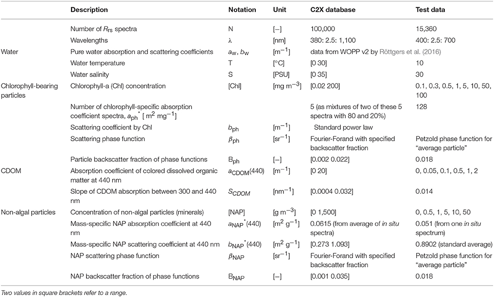
Table 1. Specifications of the two used R_rs(λ) datasets, C2X database and test data, both simulated with the “Case-2” model of HydroLight (with references in Mobley and Sundman, 2013).

The main feature of the C2X database is that it covers most water types, from clearest oceanic Case-1 waters to CDOM-dominated (extreme absorbing) and sediment-dominated (extreme scattering) Case-2 waters. For example, the total (organic and inorganic) particulate backscattering coefficient at 510 nm, b_bp(510), varies between 0.0007 and 15.4 m⁻¹ and the combined absorption coefficient of detritus and gelbstoff at 412 nm, a_dg(412), is between 0.004 and 120.2 m⁻¹. On the basis of the Xi et al. (2015) study, five fundamental spectral shapes of chlorophyll-specific absorption were selected. The five absorption spectra (of different species of algae) are supposed to have the highest potential for identification of these five different spectral groups from a remote sensing reflectance spectrum. These normalized spectra are shown in Figure 1A and stand for: (1) a “brown spectral group” representing Heterokontophyta, Dinophyta, and Haptophyta, (2) a “green spectral group” representing Chlorophyta, (3) a group for Cryptophyta, (4) a blue-green cyanobacteria, and (5) a red cyanobacteria. The first four spectra are absorption spectra from single cultures that are close to the mathematical mean for all spectra of cultures from this group (from the 128 measured culture absorption spectra). As an example, the absorption spectrum for the “brown spectral group” was chosen from all the cultures in the brown group in Figure 1B. These culture-spectra are realistic as very similar spectra can be found in the HZG in situ database (unpublished data). The spectrum of the red cyanobacteria was obtained from field measurements in the Baltic Sea during a bloom of cyanobacteria (most likely Nodularia sp.). Culture spectra (e.g., a red Synechococcus sp.) of this type mostly exhibit much higher phycobilin-related absorption peaks around 570 nm. In order to account for natural variability in the simulation for the C2X database, the actually used a_ph*(λ) spectra are always mixtures from two of the five groups with individual contributions of 80 and 20%, respectively. The total phytoplankton absorption, a_ph, is related to the spectral chlorophyll-specific absorption and chlorophyll a concentration (denoted as [Chl] hereafter), a_ph (λ) = a_ph* (λ) × [Chl]. The natural variability of phytoplankton absorption is very high (e.g., Bricaud et al., 2004); and the full range of observed natural variability is included in the simulations (Figure 2). Basis for estimating distributions, ranges, and covariances of optical properties and concentrations are several in situ datasets (e.g., Valente et al., 2016), but mainly our HZG in situ data from the North and Baltic Sea. The simulated data have been compared with in situ observations, e.g., b_bp(510) and a_dg(412) vs. different reflectance band ratios (Hieronymi et al., 2016), and we generally found a good agreement. But we have also found some discrepancies partly related to plausible measuring uncertainties and possibly due to model simplifications. In this context, it should be mentioned that the model assumptions for spectral scattering properties are identical for all five phytoplankton groups, i.e., the particle backscatter fraction depends on chlorophyll a concentration (Twardowski et al., 2001), but not on algae-specific (back-) scattering properties.

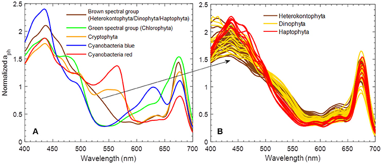
Figure 1. (A) Five area-normalized absorption spectra of phytoplankton used in R_rs(λ) simulation for the C2X database, and (B) corresponding spectra of cultures representing the “brown spectral group.”

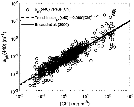
Figure 2. Phytoplankton absorption coefficient at 440 nm, a_ph(440), vs. chlorophyll a concentration [Chl] used in simulations for the C2X database. The trend line is also shown in comparison to that by Bricaud et al. (2004).

For the HydroLight simulations, the considered R_rs(λ) is fully normalized, i.e., the sun is at zenith and the viewing angle is perpendicular; the water is infinitely deep; inelastic scattering, i.e., Raman scattering and Chl and CDOM fluorescence, are taken into account. Nonetheless, how inelastic scattering processes and their natural variability influence the results is out of scope of this work. Ultimately, the C2X database built with HydroLight simulations includes in total 1 × 10⁵ R_rs(λ) spectra with five phytoplankton groups with various water optical conditions; while the test dataset includes 15,360 R_rs(λ) spectra, for 120 different water conditions ([Chl] varys from 0.1 to 100 mg m⁻³, [NAP] from 0 to 50 g m⁻³, and CDOM from 0 to 2 m⁻¹) with 128 phytoplankton absorption spectra (Table 1). The corresponding concentration values were listed in Table 1, and rational of the water condition settings was described and discussed in Xi et al. (2015) where this dataset was firstly used.

Phytoplankton Group Identification

The general scheme of the identification approach is illustrated in Figure 3. At first, all R_rs(λ) spectra are area-normalized and then second-order derivative is calculated. Details on the normalization and derivative transformation are described in Xi et al. (2015). To identify the corresponding phytoplankton groups in a test data set, each R_rs(λ) spectrum in the test data set is compared to all spectra in the C2X database using the similarity index (SI) as an angular distance (Millie et al., 1997):

where x₁ is a second-derivative spectrum of R_rs(λ) in the C2X database, and x₂ is one in the test dataset. The SI is a number between 0 and 1, where 0 indicates no similarity and 1 indicates perfect similarity between the two spectra. It is noteworthy that only the second-derivative spectra of R_rs(λ) in the range of 420–620 nm was used for SI calculation to minimize the influence of noises at shorter wavelengths, where reflectance is often low, and that of strong water absorption features at longer wavelengths (Xi et al., 2015).

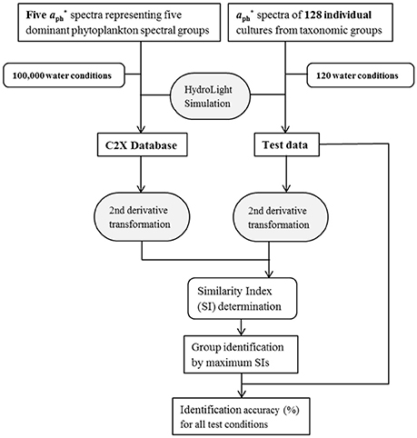
Figure 3. Flowchart showing the approach for dominant phytoplankton group identification.

This approach produces 10⁵ SI values for each spectrum of the test dataset. The first 20 spectra in the C2X database providing highest SI values for each test spectrum are selected and their corresponding known phytoplankton spectral group is recorded. The group that is dominant in these 20 spectra is taken as the identified spectral group for this test spectrum. For each test spectrum one of the five spectral groups is identified as being dominant. Each taxonomic group in the test data is represented by five to 48 R_rs(λ) spectra (from 5 to 48 different cultures), and all taxonomic groups are categorized into five spectral groups, the spectral group identification accuracy is thus determined by calculating the percentage of the correctly identified R_rs(λ) spectra in each spectral group. In the end, given that there are 120 water optical conditions in the test data, 120 values for the identification accuracy of each group are calculated.

In situ R_rs(λ) Data of Lake Taihu

An investigation campaign was carried out from 5th to 17th October 2008 in Lake Taihu (China). A set of in situ R_rs(λ) spectra was obtained by measuring the water-leaving radiances and sky radiances with a dual channel spectrometer, ASD FieldSpec Pro Dual VNIR (FieldSpec 931, ASD Inc., USA), following NASA ocean optics protocols (Mueller et al., 2003). When performing the measurements, the viewing angels of the two channels from the water surface at the zenith angle and the azimuth angle were 40° and 135°, respectively. Radiances of a 25 cm by 25 cm plaque with 25% reflectivity, water and sky radiances (each preceded by a dark offset reading) were measured and repeated five times. The measurements were performed at a location that minimized shading, reflections from superstructure, ship's wake, foam patches, and whitecaps. Moreover, the location was also pointed away from the sun to reduce the sunglint effect. Upon the upward radiance (Lu), sky radiance (Lsky), gray plaque radiance (Lplaq), and the water-air interface reflectivity determined based on the lake state at that time, R_rs(λ) were calculated referring to the method proposed by Mobley (1999). Details of the approaches for radiance measurements and R_rs(λ) calculation are illustrated in Ma et al. (2006). Water samples were taken simultaneously with the spectrometer for lab measurements of Chl, NAP, and CDOM concentrations. Absorption spectra by the total particles and the NAP were determined by quantitative filter technique (QFT) method (Mitchell, 1990) and a_ph (λ) was obtained by subtracting a_NAP(λ) from a_p(λ). a_CDOM(λ) was also measured spectrophotometrically in a 10 cm cuvette using 0.7 mm Whatman GF/F-filtered water sample pads by the same UV-2401 spectrophotometer. More details on the above determinations are described in Xi (2011).

As one of the biggest freshwater lakes in China, Lake Taihu covers an area of 2427.8 km² with highly varying water quality from area to area. Water types in Lake Taihu are mainly classified into two categories: optically deep waters (ODWs) and optically shallow waters (OSWs) (Xi, 2011). ODWs cover most area of the lake with highly eutrophicated and turbid waters and frequent occurrence of cyanobacteria blooms, while the southeastern area is mostly OSWs with clear waters and abundant aquatic plants. Data used here are from ODWs only, as R_rs(λ) from OSWs has much influence from the submerged aquatic plants and the lake bottom and are thus not suitable for use in this study. Due to the large area of the lake, water optical conditions in ODWs are also diverse. Variations of the water components are known: [Chl] varied from 4.0 to 180 mg m⁻³, [NAP] from 9.5 to 95 g m⁻³ and CDOM from 0.4 to 1.7 m⁻¹. For the present study, R_rs(λ) spectra together with other optical parameters for 66 stations in ODWs are obtained. This additional “Taihu dataset” is used to test the applicability of the presented approach in natural waters.

Results

Spectral Analysis of C2X Reflectances

The C2X database contains simulated R_rs(λ) spectra that included as model input a standard absorption spectrum for each of five different phytoplankton spectral groups. These R_rs(λ) spectra show different spectral features reflecting various water optical conditions. Prior to utilizing the C2X data in the identification approach, R_rs(λ) spectra in the database are firstly normalized and transformed to the second derivative spectra. To have an general understanding on the C2X database, representative R_rs(λ) spectra of the five phytoplankton groups and their second derivatives are selected for a few water cases. For each water case, five R_rs(λ) spectra with similar water optical conditions representing the five phytoplankton groups are chosen. Figure 4 shows examples of R_rs(λ) spectra and their second derivative spectra, for different phytoplankton groups in five water cases. The five water cases are however not exhaustive. According to Hieronymi et al. (2017), 13 different water optical classes in total are classified by a fuzzy logic classification approach, but they are not completely included here as this study is not focusing on water type interpretation. Only examples of five water cases are chosen to show spectral variations in different scenarios. These five water cases possess the following conditions:

(1) low [Chl], low [NAP], and low CDOM (Figure 4A–C);

(2) low [Chl], low [NAP], and moderate CDOM (Figure 4D–F);

(3) low [Chl], moderate [NAP], and moderate CDOM (Figure 4G–I);

(4) high [Chl], moderate [NAP], and moderate CDOM (Figure 4J–L); and

(5) moderate [Chl], extremely high [NAP], and moderate CDOM (Figure 4M–O).

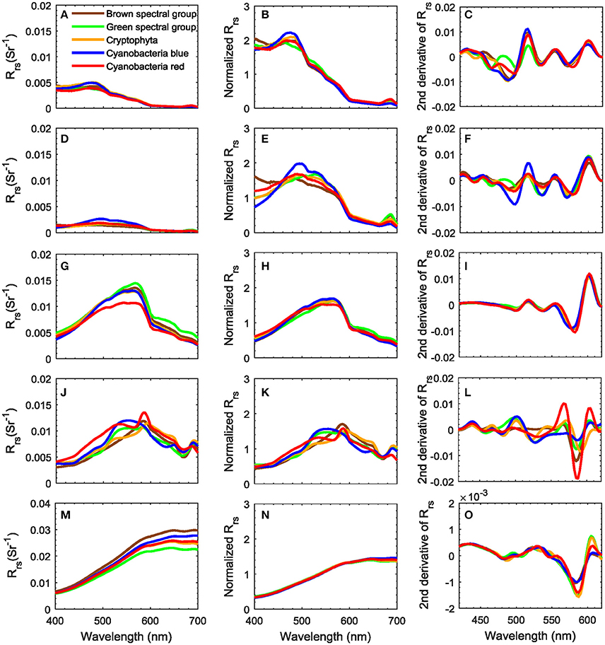
Figure 4. Representatives of R_rs(λ) spectra (first column), the corresponding area-normalized R_rs(λ) spectra (second column) and second derivative spectra (third column) for five phytoplankton spectral groups and different water conditions. (A–C) Low [Chl], [NAP], and CDOM; (D–F) low [Chl] and [NAP], moderate CDOM; (G–I) low [Chl], moderate [NAP] and CDOM; (J–L) high [Chl], moderate [NAP] and CDOM; and (M–O) moderate [Chl], extremely high [NAP], and moderate CDOM. Note that the second derivative spectra were only for 420–620 nm, i.e., the spectral range used in the identification approach.

The corresponding water optical conditions of the five water cases and the variation of water optical components are listed in Table 2. Note that the ranges of “low,” “moderate,” and “high” concentrations are a bit varying from case to case which may cause slight difference in the spectral magnitude as well as the chlorophyll fluorescence. Water case (1) represents clear Case-1 waters (Figure 4A) where phytoplankton, CDOM and pure water are the main contributors to the R_rs(λ); phytoplankton absorption contributes to the suppression at 440 nm and the reflectance in the blue spectral region is high; low scattering and the high absorption by water at red and near infrared wavelengths results in low reflectance in this region. In absorbing waters such as water case (2) where CDOM is moderate but other concentrations are low (Figure 4D), reflectance is lower in the blue band suggests a strong CDOM absorption, and the peak at about 682 nm is due to the fact that Chl fluorescence was included in the simulations. In scattering dominated waters as water case (3) (Figure 4G), NAP are the dominating component; the reflectance is high in the whole visible region and the maximum is shifted to longer wavelength with the increase of NAP concentrations; peaks and troughs attributable to pigment absorption are suppressed. In high [Chl] waters as water case (4), the contribution by different phytoplankton pigments in the R_rs(λ) spectra is clearly seen (Figure 4J), suggesting that it is relatively easy to identify phytoplankton groups in such waters. Scattering by NAP results in higher reflectance at longer wavelengths (>550 nm), therefore when sediment load is extremely high, as shown in Figure 4M, the reflectance shows an increasing pattern with wavelengths in the visible region. In NAP-dominated waters, little spectral difference can be observed among the different phytoplankton groups (Figure 4N); absorption and scattering by sediments mask the algae pigment features. This masking effect is a generally known limitation and uncertainty source for remote sensing of biomass in turbid Case-2 waters (e.g., IOCCG, 2000).

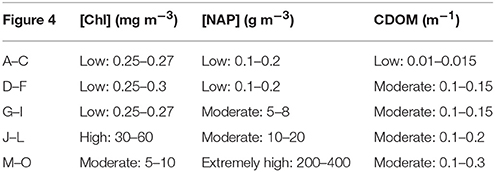
Table 2. Corresponding variations of [Chl], [NAP] and CDOM for R_rs(λ) spectra in Figure 4.

Though phytoplankton groups exhibit distinct spectral features in some water cases, the corresponding second derivative spectra of R_rs(λ) in Figure 4 (third column) show much variation in different water cases even for the same dominating phytoplankton group, due to the different contribution of other water optical constituents to the reflectance spectra. This indicates a possible difficulty in identifying phytoplankton groups for highly variable natural waters, by only inter-comparing the reflectance spectra without references. Given that, our theoretical basis is the C2X database that in the following is used as a look-up table (LUT) of standard reflectance spectra with information about the dominating phytoplankton groups, so that any test spectrum can be spectrally compared to the LUT and a certain phytoplankton group can be allocated to it. With the use of the simulated test data, the performance by the LUT identification approach can be evaluated for various water optical conditions.

Phytoplankton Spectral Group Identification

In order to investigate how accurate the phytoplankton groups can be identified under different water optical conditions, R_rs(λ) spectra of the test data are compared with those in the C2X database by following the identification approach described above. Identification accuracy based on the 120 water conditions is generated for each spectral group via the proposed approach. The identification accuracy is presented for each spectral group as a function of the different water conditions using a ternary plot (Figure 5). Since a triangular diagram displays the proportion of three variables that sum to a constant, absorption coefficients by phytoplankton and NAP are used here to represent [Chl] and [NAP], respectively. CDOM itself is typically represented by the absorption of CDOM. The sum of these three absorption coefficients can be normalized to be 1, ignoring the absorption of pure water. Their proportions for all the 120 water conditions can be well displayed in a ternary plot. [Chl] and [NAP] are thus transformed to the corresponding absorption coefficients at 440 nm, a_ph(440) and a_NAP(440), and used together with a_CDOM(440). Four hundred and forty nanometers is chosen as all components do significantly absorb light at this wavelength, and contribution by pure water is low. The transformation from [Chl] to a_ph(440) is based on the relationship shown in Figure 2: a_ph(440) = 0.06 × [Chl]^0.728 and a_NAP(440) = a_NAP*(440) × [NAP], where the mass-specific NAP absorption at 440 nm, a_NAP*(440) = 0.0615 m² g⁻¹ as shown in Table 1. Different colors and sizes of the dots are used to represent the actual [Chl] and [NAP] respectively, as the position in the ternary plot only shows each relative contribution.

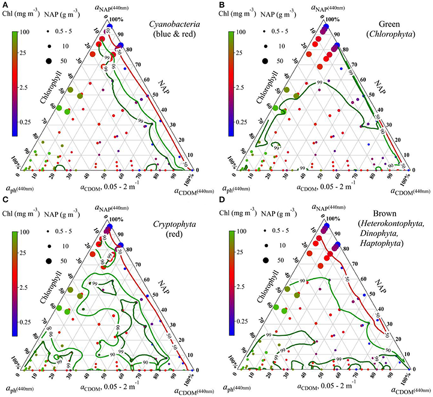
Figure 5. Ternary plots showing the identification accuracy of phytoplankton groups (A) Cyanobacteria (red and blue), (B) Chlorophyta (green spectral group), (C) Cryptophyta (red), and (D) Brown spectral group in different water conditions with respect to fractions of phytoplankton, NAP, and CDOM absorption at 440 nm: Contour lines indicate the accuracy of identification. Colors of dots indicate Chl concentrations; sizes of dots indicate NAP concentrations.

Contour lines of the identification accuracy are plotted for each spectral group (Figure 5). The contour lines indicate different distribution of the identification accuracy for the different groups. However, a main finding in common is that low identification (50% contour line) for all groups located in the plot area where [NAP] is high (bigger dots) and [Chl] (blue dots) is low. However, this is not always true. If taking a further look on the plots one can see that the identification accuracy is also dependent on the absorption contribution of each water components but not only on concentrations. In Figure 5, for simplification, blue and red cyanobacteria are combined, as they show distinct spectral features compared to other groups and their identification results are highly similar. Cyanobacteria blue and red (combined in Figure 5A) show a relatively distinct contour pattern: the contour lines are roughly parallel with low Chl contributions, e.g., the identification rate of 90% is approximately at a_ph(440) taking up only 10% of the total non-water absorption (a_ph+CDOM+NAP), and the 99% contour line is between 10 and 20%, meaning that cyanobacteria can be successfully identified when a_ph(440) takes up more than 20% of the total non-water absorption. The approach also performs well on the green spectral group (Chlorophyta), as Figure 5B shows that the identification rates falls in 90% only when [Chl] is extremely low [a_ph(440) is <5%] and [NAP] is as high as 50 g m⁻³, in all other conditions chlorophytes are correctly identified. The identification contour lines for cryptophytes in Figure 5C show more variations for different water conditions, due to the fact that there are only five cultures for Cryptophyta in the test dataset and one culture showed higher similarity with red cyanobacteria and is thus misidentified at some water conditions. This has lowered 20% of the identification rate. The overall performance of identifying species of the brown spectral group show that 90% of the cultures from Heterokontophyta, Dinophyta, and Haptophyta are correctly identified as being brown when a_ph(440) contributes more than 20% and a_NAP(440) contributes <60% to the total non-water absorption (Figure 5D).

Applicability Test Using Taihu In situ Dataset

Though the performance of using the simulated test dataset showed satisfactory results at specific water conditions, the ultimate goal of our approach is to identify phytoplankton groups by using reflectance spectra of natural waters. A set of in situ R_rs(λ) spectra of Lake Taihu is taken to perform an additional test on the applicability of the proposed approach. The second derivative spectra of in situ R_rs(λ) in 420–620 nm are compared with that in C2X database to produce highest SIs leading us to find the corresponding dominating phytoplankton groups. Results show that only two phytoplankton spectral groups are found, blue cyanobacteria and Chlorophyta, In the examined 66 stations, for 52 (80%) the dominating phytoplankton are identified as cyanobacteria (blue) and 14 (20%) as chlorophytes. Figure 6 shows the classified spectra of in situ R_rs(λ), the corresponding normalized R_rs(λ) in 400–700 nm, and the second derivative spectra. It is clearly seen that most spectra identified as Chlorophyta exhibit higher reflectance in 500–600 nm and lower chlorophyll fluorescence peaks around 690 nm, indicating higher sediment concentrations and lower Chl concentrations. On the contrary, spectra that are identified as cyanobacteria show distinct absorption peaks at 675 nm and more pronounced fluorescence (Figure 6B). Table 3 lists the identification results for Lake Taihu when stations are selected by different [Chl], showing that the identification rate of cyanobacteria increases with the increasing minimum [Chl]: 90% when [Chl] > 10 mg m⁻³, 98% when [Chl] > 20 mg m⁻³, and 100% when [Chl] > 30 mg m⁻³.

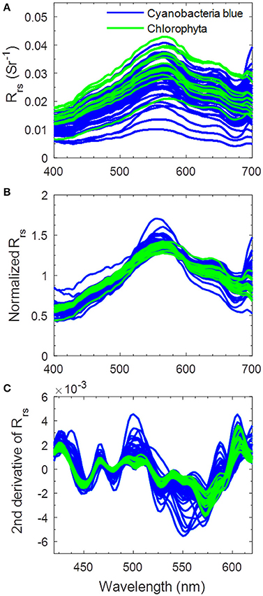
Figure 6. Phytoplankton-group-classified spectra of (A) in situ R_rs(λ) in Lake Taihu in 400–700 nm, (B) the corresponding area-normalized R_rs(λ), and (C) second derivative spectra in 420–620 nm.

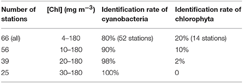
Table 3. Phytoplankton groups identification in Lake Taihu with different [Chl] ranges.

It has been known in the context that [Chl] has an order of two in magnitude, and water optical conditions highly varied from station to station in Lake Taihu. The information we had from the campaign was that in waters where [Chl] was roughly 30 mg m⁻³ or higher, cyanobacteria aggregated obviously and were the dominating group. Whereas, lower [Chl] waters could either be green algae or cyanobacteria dominated according to the identification. To explore whether the two identified groups are relating to the absorption contributions of each water component, proportions of a_ph(440), a_NAP(440), and a_CDOM(440) to the total non-water absorption at 440 nm were statistically summarized for cyanobacteria identified stations and green algae identified stations, respectively (Table 4). The overall [Chl] and contribution of aph(440) at cyanobacteria dominating stations are higher than that at green algae dominating stations. Mean a_ph(440) contribution is 16.1% for cyanobacteria while only 9.8% for green algae. a_NAP(440) contribution shows the opposite with a_ph(440), with lower mean value (58.1%) for cyanobacteria but slightly higher for green algae; no difference is found in CDOM contribution between the two groups. These statistical results in Table 4 also reveal that CDOM has little influence in the identification, in agreement with results from the simulated test dataset. Lower phytoplankton contribution in green algae dominating stations might suggest that the identification of green algae is less accurate.

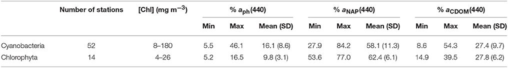
Table 4. Identified phytoplankton groups with relation to contributions of a_ph(440), a_NAP(440), and a_CDOM(440) to the total non-water absorption.

Discussion

Simulated C2X Data

Generally, the simulated reflectance spectra in the C2X database are plausible and fit to in situ measurements. For example, many lakes have signal-dominating CDOM fractions and exhibit reflectance spectra as shown in Figure 4D (e.g., Eleveld et al., 2017) and Figure 4M shows similar spectra as measured in a turbid estuary (e.g., Knaeps et al., 2012). Nonetheless, the simulations are based on some spectral assumptions that may lead to inaccuracy and therefore uncertainties in the group identification. One simplification regards the scattering properties of phytoplankton; some natural variability is included in the simulations, but due to the lack of reliable specific information, all phytoplankton groups are modeled with the same scattering assumptions. But due to different particle shapes and size distribution, it is evident that the spectral scattering properties vary (e.g., Morel, 1987; Evers-King et al., 2014; Harmel et al., 2016). Robertson Lain et al. (2017) showed the potentially considerable influence of different phytoplankton phase functions on modeled remote sensing reflectance over the entire visible range. A second point of model uncertainties, particularly in the range 650–700 nm, regards inelastic scattering effects such as CDOM and phytoplankton fluorescence; in nature, the quantum yield efficiency of phytoplankton varies significantly depending on nutrient- and light-availability and algae species (e.g., Greene et al., 1994). However, in the HydroLight simulations, the standard quantum yield efficiency was used.

Identification Approach and Its Skill

The proposed approach was chosen for phytoplankton group identification based on the idea of whether we can identify phytoplankton groups by only knowing R_rs(λ), which is a directly obtained parameter from satellite sensors. All other inversion models require information on water inherent optical properties and the retrieval accuracy can be various (e.g., Werdell et al., 2014; Wang et al., 2016). In our previous study, we have made a performance comparison between using R_rs(λ) directly and using QAA-inverted absorption spectra from R_rs(λ) for phytoplankton group differentiation (Xi et al., 2015). Results show that the inverted absorption spectra performed less precise compared to the R_rs(λ). Due to the retrieval algorithm constraints, pigment information in the derived absorption spectra might be lost or distorted as theoretical or empirical relationships between the IOPs and AOPs are normally used in the retrieval algorithm. Upon the simulated extensive R_rs(λ) database, a direct comparison in spectral shapes between the second derivatives of a test R_rs(λ) spectrum and that of the spectra in the database is carried out by the current approach, omitting the knowledge of optical properties as well as the retrieval errors introduced by inversions. The benefit of this approach would be that we provide a straightforward way allowing us to know the dominant phytoplankton group (if it is one of the five) once R_rs(λ) is obtained from either in situ measurements or hyperspectral satellite data.

Skill of the proposed approach varies in different water conditions. Results derived by using the test dataset for various water optical properties indicated that the identification accuracy was highly subject to the water optical conditions; the identification was effective for waters with high phytoplankton contribution but less effective in NAP dominated waters, whereas CDOM has little influence even when it is extremely high. It is not only in agreement with the results by Xi et al. (2015) that phytoplankton groups differentiation is unsuccessful in waters with [Chl] lower than 1 mg m⁻³, but also suggested the low efficiency in high [NAP] waters. However, regarding the optical boundaries of the successful identifications, it should be clarified that the accuracy of the identification is not only dependent on the concentrations of water components but also on the contribution of absorption by each water component to the total absorption. That means the identification accuracy can possibly be high both in case 1 clear waters and in highly turbid productive (phytoplankton abundant) waters. There are no clear concentration boundaries. And the optical boundaries in terms of absorption contribution are nicely shown in the ternary plots (Figure 5). Regarding this matter, ternary plots exhibit clearly the contour line distribution of the identification accuracy for all water optical conditions generated by 120 points representing 120 water optical conditions. We can roughly wrap up some general findings from the ternary plots, that are—the identification accuracy is higher than 90% when the absorption by phytoplankton is taking up more than 20% and the NAP contribution is <60% to the total absorption; for the groups of cyanobacteria and green algae, the identification accuracy is even higher at the above boundaries.

Though there were only 120 water optical conditions considered in the test dataset, it included most of the natural aquatic environment from clear to moderate turbid and productive waters. The findings have provided us a basic knowledge that the proposed approach for phytoplankton group identification performs well except for waters where phytoplankton contribution to the overall absorption is low and for NAP dominated waters. Regarding the five spectral groups included in C2X database, they are not exhaustive but are chosen to represent natural common groups. In addition, due to modeling and computing constraints, the phytoplankton groups that were taken into account in the simulation have to be representative and the number of the groups should be as low as possible to allow extensive simulations. This database is however adjustable, when absorption features of other phytoplankton groups (or species with typical features) are important.

Phytoplankton Group Identification in Lake Taihu

To test the applicability of the proposed approach in natural waters, in situ remote sensing reflectance data obtained from Lake Taihu were used. Though lacking the information of dominant phytoplankton species or pigment analysis for this campaign in October 2008, previous investigations on the phytoplankton community and composition in Lake Taihu can be taken as reference. Chen et al. (2003) revealed that phytoplankton groups commonly observed in Lake Taihu are cyanobacteria, Chlorophyta, Bacillariophyta, and flagellates. A study on phytoplankton community structure succession in Lake Taihu from 1992 to 2012 by Deng et al. (2014) showed that Cryptomonas (Cryptophyta) was the dominant species in spring during the early 1990s. Dominance then shifted to Ulothrix (Chlorophyta) in 1996 and 1997. However, Cryptomonas again dominated in 1999, 2000, and 2002, with Ulothrix regaining dominance from 2003 to 2006. The bloom-forming cyanobacterial species Microcystis sp., a typical blue cyanobacteria, dominated in 1995, 2001, and 2007–2012. Another study revealed that Microcystis sp. is the most commonly seen cyanobacteria species, approximately taking up 85% of algae biomass and forming algal blooms each summer (Zhu et al., 2007). More importantly, a year-long investigation in dominant phytoplankton species from October 2008 to October 2009 conducted in the lake showed that Microcystis sp. dominated in October 2008, when our in situ data was collected, contributing more than 90% of total biovolume in most area of the lake, coexisted with minor portion of the cyanobacteria Dolichospermum flos-aquae and the diatom Cyclotella meneghiniana (Ai et al., 2015). Our identification results showed good agreement with these investigations, except that chlorophytes were identified as the dominant group at some stations when [Chl] was moderate. Comparison in absorption contributions between cyanobacteria and green algae identified stations shows that phytoplankton contribute <10% on average to the total non-water absorption at green algae identified stations (Table 4), leading to lower identification accuracy as indicated in Figure 5. It is highly likely that this is a misinterpretation, as still cyanobacteria were codominant.

The in situ data of Lake Taihu are used as a first example. Coinciding data of spectral reflectance and information of phytoplankton taxonomic composition are still quite rare. However, this first example has given optimistic outcome and the fact that the approach is applicable in this optically complex lake. More datasets in different water types are under collection and processing, with expectations to testify further the identification approach in more natural waters.

Conclusions and Outlook

A database of R_rs(λ) spectra, C2X database, based on five phytoplankton groups was built using HydroLight simulations for various water optical conditions. A similarity-index approach was proposed to identify phytoplankton groups, using remote sensing reflectance spectra only, by spectrally comparing an input test spectra with the R_rs(λ) in C2X database. The performance of the approach was tested using another simulated R_rs(λ) dataset with 128 spectra of phytoplankton algae from six taxonomic groups arranged into five spectral groups. For 120 water optical conditions, the identification was high at most occasions except for waters with a low phytoplankton contribution and for waters dominated by NAP. Whereas, the influence of CDOM is less pronounced and only significant at extremely high level. Though the proposed approach was based on simulated datasets, its applicability in natural waters was also tested by using in situ R_rs(λ) spectra from Lake Taihu, China. Despite of possibly wrong identification of chlorophytes that could not be validated, cyanobacteria were successfully identified in Lake Taihu as a dominating group in high [Chl] waters, proving the applicability of the approach in natural waters when a single group is dominating.

The current approach is only capable of identifying spectral groups that are already presented in the C2X database. However, the database can be expanded by running the same HydroLight simulations with different absorption characteristics of other phytoplankton groups. The following aspects might be worth to investigate: (1) more validation with in situ data and measurements; (2) applicability in extreme events such as floating algae in highly turbid waters; (3) determination on the required or lowest spectral resolution for a wider use of hyperspectral R_rs(λ); and (4) examination of using hyperspectral satellite data in consideration of influences of radiometric, spectral, and atmospheric effects on R_rs(λ) from the space.

Author Contributions

HX carried out the data analysis and the approach development with guidance from RR. MH simulated the hyperspectral remote sensing reflectance for the C2X database and the test data using HydroLight. HX drafted the main manuscript and MH refined the simulation part in Data and method. MH, RR, and HK all provided comments and suggestions and revised the manuscript.

Funding

The work of HX is supported by the project “Preparations for the scientific use of the EnMAP data: Coastal and inland waters (50EE1257).” EnMAP is funded under the DLR Space Administration with resources from the German Federal Ministry of Economic Affairs and Energy. MH is partly supported by ESA through a Living Planet Fellowship. The C2X database was established by MH in the ESA SEOM C2X project (ESA ESRIN/C-No. 4000113691/15/I-LG). We thank ESA for sponsoring the publication.

Conflict of Interest Statement

The authors declare that the research was conducted in the absence of any commercial or financial relationships that could be construed as a potential conflict of interest.

Acknowledgments

We are thankful to Stephen Gehnke for measuring absorption spectra of various phytoplankton cultures. The in situ data of Lake Taihu was collected and measured by the Nanjing Institute of Geography and Limnology, Chinese Academy of Sciences. We thank Dr. Hongtao Duan and Prof. Yuanzhi Zhang for providing in situ dataset under the support of the Provincial National Science Foundation of Jiangsu of China (BK20160049) and the National Key Research and Development Program of China (2016YFC1402000). The Open Fund at Jiangsu Key Laboratory of Remote Sensing of Ocean Dynamics and Acoustics in NUIST (KHYS1403) is also acknowledged. We finally thank the two reviewers for providing constructive comments to improve the manuscript.

References

Ai, Y., Bi, Y., and Hu, Z. (2015). Response of predominant phytoplankton species to anthropogenic impacts in Lake Taihu. J. Freshw. Ecol. 30, 99–112. doi: 10.1080/02705060.2014.992052
Aiken, J., Hardman-Mountford, N. J., Barlow, R., Fishwick, J., Hirata, T., and Smyth, T. (2008). Functional links between bioenergetics and bio-optical traits of phytoplankton taxonomic groups: an verarching hypothesis with applications for ocean colour remote sensing. J. Plankton Res. 30, 165–181. doi: 10.1093/plankt/fbm098
Alvain, S., Loisel, H., and Dessailly, D. (2012). Theoretical analysis of ocean color radiances anomalies and implications for phytoplankton groups detection in case 1 waters. Opt. Express 20, 1070–1083. doi: 10.1364/OE.20.001070
Alvain, S., Moulin, C., and Dandonneau, Y. (2008). Seasonal distribution and succession of dominant phytoplankton groups in the global ocean: a satellite view. Glob. Biogeochem. Cycles 22, GB3001. doi: 10.1029/2007GB003154
Alvain, S., Moulin, C., Dandonneau, Y., and Breon, F. M. (2005). Remote sensing of phytoplankton groups in case 1 waters from global SeaWiFS imagery. Deep Sea Res. Part I 1, 1989–2004. doi: 10.1016/j.dsr.2005.06.015
Astoreca, R., Rousseau, V., Ruddick, K., Knechciak, C., von Mol, B., Parent, J., et al. (2009). Development and application of an algorithm for detecting Phaeocystis globosa blooms in the Case 2 Southern North Sea waters. J. Plankton Res. 31, 287–300. doi: 10.1093/plankt/fbn116
Barnsley, M. J., Settle, J. J., Cutter, M. A., Lobb, D. R., and Teston, F. (2004). The PROBA/CHRIS MISSION: a low-cost smallsat for hyperspectral multiangle observations of the earth surface and atmosphere. IEEE Trans. Geosci. Remote Sens. 42, 1512–1520. doi: 10.1109/TGRS.2004.827260
Bracher, A., Bouman, H., Brewin, R. J., Bricaud, A., Brotas, V., Ciotti, A. M., et al. (2017). Obtaining phytoplankton diversity from ocean color: a scientific roadmap for future development. Front. Mar. Sci. 4:55. doi: 10.3389/fmars.2017.0005
Bracher, A., Vountas, M., Dinter, T., Burrows, J. P., Röttgers, R., and Peeken, I. (2009). Quantitative observation of cyanobacteria and diatoms from space using PhytoDOAS on SCIAMACHY data. Biogeosciences 6, 751–764. doi: 10.5194/bg-6-751-2009
Brewin, R. J. W., Sathyendranath, S., Jackson, T., Barlow, R., Brotas, V., Airs, R., et al. (2015). Influence of light in the mixed-layer on the parameters of a three-component model of phytoplankton size class. Remote Sens. Environ. 168, 437–450. doi: 10.1016/j.rse.2015.07.004
Bricaud, A., Claustre, H., Ras, J., and Oubelkheir, K. (2004). Natural variability of phytoplanktonic absorption in oceanic waters: influence of the size structure of algal populations. J. Geophys. Res. 109, C11. doi: 10.1029/2004JC002419
C2X (2015). ESA SEOM C2X Project ‘Case-2 Extreme Waters’. Available online at: http://seom.esa.int/page_project014.php
Chen, Y., Qin, B., Teubner, K., and Dokulil, M. T. (2003). Long-term dynamics of phytoplankton assemblages:Microcystis-domination in Lake Taihu, a large shallow lake in China. J. Plankton Res. 25, 445–453. doi: 10.1093/plankt/25.4.445
Ciotti, A. M., and Bricaud, A. (2006). Retrievals of a size parameter for phytoplankton and spectral light absorption by colored detrital matter from water-leaving radiances at SeaWiFS channels in a continental shelf region of Brazil. Limnol. Oceanogr. Methods 4, 237–253. doi: 10.4319/lom.2006.4.237
Corson, M. R., Korwan, D. R., Lucke, R. L., Snyder, W. A., and Davis, C. O. (2008). “The Hyperspectral Imager for the Coastal Ocean (HICO) on the International Space Station,” in IGARSS 2008 - 2008 IEEE International Geoscience and Remote Sensing Symposium, Vol. 4 (Boston, MA), IV-101–IV-104. doi: 10.1109/IGARSS.2008.4779666
Craig, S. E., Lohrenz, S. E., Lee, Z., Mahoney, K. L., Kirkpatrick, G. J., Schofield, O. M., et al. (2006). Use of hyperspectral remote sensing reflectance for detection and assessment of the harmful alga, Karenia brevis. Appl. Opt. 45, 5414–5425. doi: 10.1364/AO.45.005414
Deng, J., Qin, B., Paerl, H. W., Zhang, Y., Wu, P., Ma, J., et al. (2014). Effects of nutrients, temperature and their interactions on spring phytoplankton community succession in Lake Taihu, China. PLoS ONE 9:e113960. doi: 10.1371/journal.pone.0113960
Eleveld, M. A., Ruescas, A. B., Hommersom, A., Moore, T. S., Peters, S. W., and Brockmann, C. (2017). An optical classification tool for global lake waters. Remote Sens. 9:420. doi: 10.3390/rs9050420
Evers-King, H., Bernard, S., Lain, L. R., and Probyn, T. A. (2014). Sensitivity in reflectance attributed to phytoplankton cell size: forward and inverse modelling approaches. Opt. Express 22, 11536–11551. doi: 10.1364/OE.22.011536
Foerster, S., Carrère, V., Rast, M., and Staenz, K. (2015). Preface: the Environmental Mapping and Analysis Program (EnMAP) Mission: preparing for its scientific exploitation. Remote Sens. 8:957. doi: 10.3390/rs8110957
Folkman, M. A., Pearlman, J., Liao, L. B., and Jarecke, P. J. (2001). “EO-1/Hyperion hyperspectral imager design development characterization and calibration,” in Proceedings SPIE 4151, Hyperspectral Remote Sensing of the Land and Atmosphere (Sendai), 40.
Greene, R. M., Kolber, Z. S., Swift, D. G., Tindale, N. W., and Falkowski, P. G. (1994). Physiological limitation of phytoplankton photosynthesis in the eastern equatorial Pacific determined from variability in the quantum yield of fluorescence. Limnol. Oceanogr. 39, 1061–1074. doi: 10.4319/lo.1994.39.5.1061
Gregg, W., and Rousseaux, C. (2017). Simulating PACE Global Ocean Radiances. Front. Mar. Sci. 4:60. doi: 10.3389/fmars.2017.00060
Guanter, L., Kaufmann, H., Segl, K., Foerster, S., Rogass, C., Chabrillat, S., et al. (2015). The EnMAP spaceborne imaging spectroscopy mission for Earth Observation. Remote Sens. 7, 8830–8857. doi: 10.3390/rs70708830
Harmel, T., Hieronymi, M., Slade, W., Röttgers, R., Roullier, F., and Chami, M. (2016). Laboratory experiments for inter-comparison of three volume scattering meters to measure angular scattering properties of hydrosols. Opt. Express 24, A234–A256. doi: 10.1364/OE.24.00A234
Hieronymi, M., Krasemann, H., Müller, D., Brockmann, C., Ruescas, A., Stelzer, K., et al. (2016). “Ocean colour remote sensing of extreme case-2 waters,” in Proceedings of Living Planet Symposium (Prague: ESA SP-740).
Hieronymi, M., Müller, D., and Doerffer, R. (2017). The OLCI Neural Network Swarm (ONNS): a bio-geo-optical algorithm for open ocean and coastal waters. Front. Mar. Sci. 4:140. doi: 10.3389/fmars.2017.00140
Hirata, T., Aiken, J., Hardman-Mountford, N., Smyth, T. J., and Barlow, R. G. (2008). An absorption model to determine phytoplankton size classes from satellite ocean color. Remote Sens. Environ. 112, 3153–3159. doi: 10.1016/j.rse.2008.03.011
Hunter, P. D., Tyler, A. N., Présing, M., Kovács, A. W., and Preston, T. (2008). Spectral discrimination of phytoplankton colour groups: the effect of suspended particulate matter and sensor spectral resolution. Remote Sens. Environ. 112, 1527–1544. doi: 10.1016/j.rse.2007.08.003
Isada, T., Hirawake, T., Kobayashi, T., Nosake, Y., Natsuike, M., Imai, I., et al. (2015). Hyperspectral optical discrimination of phytoplankton community structure in Funka Bay and its implications for ocean color remote sensing of diatoms. Remote Sens. Environ. 159, 134–151. doi: 10.1016/j.rse.2014.12.006
IOCCG (2000). “Remote sensing of ocean colour in coastal, and other optically-complex, waters,” in Reports of the International Ocean-Colour Coordinating Group, ed S. Sathyendranath (Dartmouth: IOCCG).
IOCCG (2014). “Phytoplankton functional types from space,” in Reports of the International Ocean-Color Coordinating Group, No. 15, ed S. Sathyendranath (Dartmouth: IOCCG).
Kim, Y., Yoo, S., and Son, Y. B. (2016). Optical discrimination of harmfulCochlodinium polykrikoidesblooms in Korean coastal waters. Opt. Express 24, A1471–A1488. doi: 10.1364/OE.24.0A1471
Knaeps, E., Dogliotti, A. I., Raymaekers, D., Ruddick, K., and Sterckx, S. (2012). In situ evidence of non-zero reflectance in the OLCI 1020nm band for a turbid estuary. Remote Sens. Environ. 120, 133–144. doi: 10.1016/j.rse.2011.07.025
Kostadinov, T. S., Siegel, D. A., and Maritorena, S. (2009). Retrieval of the particle size distribution from satellite ocean color observations. J. Geophys. Res. 114, C09015. doi: 10.1029/2009JC005303
Lee, C. M., Cable, M. L., Hook, S. J., Green, R. O., Ustin, S. L., Mandl, D., et al. (2015). An introduction to the NASA Hyperspectral InfraRed Imager (HyspIRI) mission and preparatory activities. Remote Sens. Environ. 167, 6–19. doi: 10.1016/j.rse.2015.06.012
Lorenzoni, L., Toro-Farmer, G., Varela, R., Guzman, L., Rojas, J., Montes, E., et al. (2015). Characterization of phytoplankton variability in the Cariaco Basin using spectral absorption, taxonomic and pigment data. Remote Sens. Environ. 167, 259–268. doi: 10.1016/j.rse.2015.05.002
Lubac, B., Loisel, H., Guiselin, N., Astoreca, R., Artigas, L. F., and Meriaux, X. (2008). Hyperspectral and multispectral ocean color inversions to detect Phaeocystis globosa blooms in coastal waters. J. Geophys. Res. 113, C06026. doi: 10.1029/2007JC004451
Ma, R., Tang, J., and Dai, J. (2006). Bio-optical model with optical parameter suitable for Taihu Lake in water colour remote sensing. Int. J. Remote Sens. 27, 4305–4328. doi: 10.1080/01431160600857428
Meini, M., Fossati, E., Giunti, L., Molina, M., Formaro, R., Longo, F., et al. (2015). “The PRISMA mission hyperspectral payload,” in IAC-15-B1.3.7, 66th International Astronautical Congress (Jerusalem).
Michel, S., Lefèvre-Fonollosa, M., and Hsford, S. (2011). “HYPXIM–A hyperspectral satellite defined for science, security and defence users,” in 3rd Workshop on Hyperspectral Image and Signal Processing: Evolution in Remote Sensing (WHISPERS) (Lisbon). doi: 10.1109/WHISPERS.2011.6080864
Millie, D. F., Schofield, O. M., Kirpatrick, G. J., Johnsen, G., Tester, P. A., and Vinyard, B. T. (1997). Detection of harmful algal blooms using photopigments and absorption signatures: a case study of the Florida red tide dinoflagellate, Gymnodinium breve. Limnol. Oceanogr. 42, 1240–1251. doi: 10.4319/lo.1997.42.5_part_2.1240
Mitchell, B. G. (1990). “Algorithms for determining the absorption coefficient of aquatic particulates using the quantitative filter technique (QFT),” in Ocean Optics X (Orlando, FL: USA SPIE), 137–148. doi: 10.1117/12.21440
Mobley, C. D. (1994). Light and Water: Radiative Transfer in Natural Waters. San Diego, CA: Academic Press.
Mobley, C. D. (1999). Estimation of the remote-sensing reflectance from above-surface measurements. Appl. Opt. 38, 7442–7455. doi: 10.1364/AO.38.007442
Mobley, C. D., and Sundman, L. K. (2013). HydroLight 5.2 - EcoLight 5.2 Technical Documentation. Sequoia Scientific, Inc.
Morel, A. (1987). Chlorophyll-specific scattering coefficient of phytoplankton. A simplified theoretical approach. Deep Sea Res. Part A Oceanogr. Res. Pap. 34, 1093–1105. doi: 10.1016/0198-0149(87)90066-5
Mouw, C. B., Hardman-Mountford, N. J., Alvain, S., Bracher, A., Brewin, R. W., Bricaud, A., et al. (2017). A consumer's guide to satellite remote sensing of multiple phytoplankton groups in the global ocean. Front. Mar. Sci. 4:41. doi: 10.3389/fmars.2017.00041
Mouw, C. B., and Yoder, J. A. (2010). Optical determination of phytoplankton size composition from global SeaWiFSimagery, J. Geophys. Res. 115, C12018. doi: 10.1029/2010JC006337
Mueller, J. L., Fargion, G. S., and McClain, C. R. (2003). Ocean Optics Protocols for Satellite Ocean Color Sensor Validation, Vol. 1–4. Greenbelt, MD: NASA Goddard Space Flight Center.
Nair, A., Sathyendranath, S., Platt, T., Morales, J., Stuart, V., Forget, M.-H. E., et al. (2008). Remote sensing of phytoplankton functional types. Remote Sens. Environ. 112, 3366–3375. doi: 10.1016/j.rse.2008.01.021
Robertson Lain, L., Bernard, S., and Matthews, M. W. (2017). Understanding the contribution of phytoplankton phase functions to uncertainties in the water colour signal. Opt. Express 25, A151–A165. doi: 10.1364/OE.25.00A151
Röttgers, R., Doerffer, R., McKee, D., and Schönfeld, W. (2016). The Water Optical Properties Processor (WOPP): Pure Water Spectral Absorption, Scattering, and Real Part of Refractive Index Model. ATBD, Issue 1.8, ESA Water Radiance project.
Röttgers, R., Häse, C., and Doerffer, R. (2007). Determination of the particulate absorption of microalgae using a point-source integrating-cavity absorption meter: verification with a photometric technique, improvements for pigment bleaching and correction for chlorophyll fluorescence. Limnol. Oceanogr. Methods 5, 1–12. doi: 10.4319/lom.2007.5.1
Sadeghi, A., Dinter, T., Vountas, M., Taylor, B. B., Soppa, M. A., Peeken, I., et al. (2012). Improvement to the PhytoDOAS method for identification of coccolithophores using hyper-spectral satellite data. Ocean Sci. 8, 1055–1070. doi: 10.5194/os-8-1055-2012
Taylor, B. B., Torrecilla, E., Bernhardt, A., Taylor, M. H., Peeken, I., Röttgers, R., et al. (2011). Bio-optical provinces in the eastern Atlantic Ocean and their biogeographical relevance. Biogeosciences 8, 3609–3629. doi: 10.5194/bg-8-3609-2011
Torrecilla, E., Stramski, D., Reynolds, R. A., Millán-Núñez, E., and Piera, J. (2011). Cluster analysis of hyperspectral optical data for discriminating phytoplankton pigment assemblages in the open ocean. Remote Sens. Environ. 115, 2578–2593. doi: 10.1016/j.rse.2011.05.014
Twardowski, M. S., Boss, E., Macdonald, J. B., Pegau, W. S., Barnard, A. H., and Zaneveld, J. R. V. (2001). A model for estimating bulk refractive index from the optical backscattering ratio and the implications for understanding particle composition in case I and case II waters. J. Geophys. Res. 106, 14129–14142. doi: 10.1029/2000JC000404
Uitz, J., Stramski, D., Reynolds, R. A., and Dubranna, J. (2015). Assessing phytoplankton community composition from hyperspectral measurements of phytoplankton absorption coefficient and remote-sensing reflectance in open-ocean environments. Remote Sens. Environ. 171, 58–74. doi: 10.1016/j.rse.2015.09.027
Valente, A., Sathyendranath, S., Brotas, V., Groom, S., Grant, M., Taberner, M., et al. (2016). A compilation of global bio-optical in situ data for ocean-colour satellite applications. Earth Syst. Sci. Data 8, 235–252. doi: 10.5194/essd-8-235-2016
Wang, G., Lee, Z., Mishra, D. R., and Ma, R. (2016). Retrieving absorption coefficients of multiple phytoplankton pigments from hyperspectral remote sensing reflectance measured over cyanobacteria bloom waters. Limnol. Oceanogr. Methods 14, 432–447. doi: 10.1002/lom3.10102
Werdell, P. J., Roesler, C. S., and Goes, J. I. (2014). Discrimination of phytoplankton functional groups using an ocean reflectance inversion model. Appl. Opt. 53, 4833–4849. doi: 10.1364/AO.53.004833
Wolanin, A., Soppa, M. A., and Bracher, A. (2016). Investigation of spectral band requirements for improving retrievals of phytoplankton functional types. Remote Sens. 8:871. doi: 10.3390/rs8100871
Xi, H. (2011). Water Optical Properties and Water Color Remote Sensing in Optically Deep and Shallow Waters of Lake Tahu, China. Dissertation, The Chinese University of Hong Kong, Hong Kong.
Xi, H., Hieronymi, M., Röttgers, R., Krasemann, H., and Qiu, Z. (2015). Hyperspectral differentiation of phytoplankton taxonomic groups: a comparison between using remote sensing reflectance and absorption spectra. Remote Sens. 7, 14781–14805. doi: 10.3390/rs71114781
Zhu, G., Qin, B., Gao, G., Zhang, L., Luo, L., and Zhang, Y. (2007). “Effects of hydrodynamics on phosphorus concentrations in water of Lake Taihu, a large, shallow, eutrophic lake of China,” in Eutrophication of Shallow Lakes with Special Reference to Lake Taihu, China, eds B. Qin, Z. Liu, and K. Havens (Dordrecht: Netherlands Springer), 53–61. doi: 10.1007/978-1-4020-6158-5_6
Keywords: ocean color, remote sensing, phytoplankton spectral groups, light absorption, extreme case-2 waters
Citation: Xi H, Hieronymi M, Krasemann H and Röttgers R (2017) Phytoplankton Group Identification Using Simulated and In situ Hyperspectral Remote Sensing Reflectance. Front. Mar. Sci. 4:272. doi: 10.3389/fmars.2017.00272
Received: 15 March 2017; Accepted: 07 August 2017;
Published: 22 August 2017.
Edited by:
Astrid Bracher, Alfred-Wegener-Institute Helmholtz Center for Polar and Marine Research, GermanyReviewed by:
Maycira Costa, University of Victoria, CanadaAleksandra Wolanin, Helmholtz-Zentrum Potsdam Deutsches Geoforschungszentrum (GFZ), Germany
Copyright © 2017 Xi, Hieronymi, Krasemann and Röttgers. This is an open-access article distributed under the terms of the Creative Commons Attribution License (CC BY). The use, distribution or reproduction in other forums is permitted, provided the original author(s) or licensor are credited and that the original publication in this journal is cited, in accordance with accepted academic practice. No use, distribution or reproduction is permitted which does not comply with these terms.
*Correspondence: Hongyan Xi, hongyan.xi@hzg.de