Fe-Binding Dissolved Organic Ligands in the Oxic and Suboxic Waters of the Black Sea

Introduction

The Black Sea is the largest permanently anoxic basin on Earth. It is vertically stratified, caused by dense Mediterranean seawater that sinks as it enters the basin via the Bosporus, flowing below the less dense surface waters that are strongly influenced by river input. A consequence of the strong vertical stratification is a permanent halocline between 50 and 120 m that separates the underlying anoxic layer, containing high sulfide concentrations, from the overlying oxygenated surface layer (OL); between them is a suboxic zone (Sorokin, 2002a,b; Pakhomova et al., 2014; Margolin et al., 2016). The vertical diffusive flux of oxygen from the OL to the underlying suboxic zone is insufficient to meet the oxygen consumption demands for the degradation of sinking organic material. The suboxic zone, or redoxcline, is characterized by steep gradients of physicochemical properties with large consequences for microbial, physical and chemical processes. These processes in turn affect the solubility of Fe, which varies strongly along this redoxcline (Lewis and Landing, 1991; Dellwig et al., 2010), and other redoxcline environments (Dyrssen and Kremling, 1990; Van Cappellen and Wang, 1996; Taylor et al., 2001; Dellwig et al., 2010). As oxygen decreases in concentration, Fe(III) is reduced to Fe(II), increasing its solubility. In the anoxic water below the redoxcline, the solubility of Fe(II) decreases as sulfide concentrations increase, resulting in Fe precipitation (Lewis and Landing, 1991).

In the OL, the concentration of dissolved Fe (DFe) depends on external sources like dust and rivers, and on internal processes such as the dissolution of Fe-containing particles, and the presence of Fe-binding dissolved organic ligands (Rue and Bruland, 1995; Liu and Millero, 2002; Rijkenberg et al., 2006a,b; 2008; Wagener et al., 2008; Croot and Heller, 2012; Gledhill and Buck, 2012). Fe-binding dissolved organic ligands form a tiny part (<0.1%), of the dissolved organic carbon (DOC) pool, and are not well defined (Gledhill and Buck, 2012; and references herein). They can consist of highly specific Fe-binding siderophores, humic substances or polysaccharides, existing in either the truly dissolved (<0.02 μm) or colloidal (>0.02 and < 0.2 μm) phases (Bergquist et al., 2007; Thuróczy et al., 2010, 2011; Hassler et al., 2015). Siderophores are produced by bacteria as a response to Fe stress (Macrellis et al., 2001; Gledhill et al., 2004; Martinez and Butler, 2007; Mawji et al., 2011), whereas humic substances are expected to exist mostly in coastal areas and near rivers and estuaries (Laglera and van den Berg, 2009; Batchelli et al., 2010). Fe-binding dissolved organic ligands can also be produced during zooplankton grazing (Sato et al., 2007; Sarthou et al., 2008).

DOC concentrations in the OL range from ~125 μM near the OL-suboxic zone boundary to >180 μM at the surface (Ducklow et al., 2007; Margolin et al., 2016), compared to ~75 μM at the ocean surface (Hansell et al., 2009). In the OL below the euphotic zone, aerobic mineralization of organic matter regenerates inorganic nutrients and metals, such as Fe (Boyd et al., 2010), and probably also Fe-binding dissolved organic ligands (Witter et al., 2000; Gerringa et al., 2006; Gledhill and Buck, 2012). DOC is introduced into the Black Sea from two major sources: one is rivers enriched with terrigenous DOC with concentrations of ~300 μM (Cauwet et al., 2002; Saliot et al., 2002); the second is the Sea of Marmara, bringing moderate concentrations (~70 μM) via the Bosporus Strait (Polat and Tuğrul, 1995; Margolin et al., 2016). Thus, there is a relatively high content of humic substances compared to the oceans, which might have consequences for the concentrations and characteristics of the Fe-binding dissolved organic ligands in the Black Sea.

As far as we know, Fe-binding dissolved organic ligands have not yet been studied in the Black Sea, although Lewis and Landing (1991) recognized that colloidal and organically-complexed Fe species of humic origin accounted for 10–30% of the DFe in the OL. We expect that the organic complexation of Fe is an important factor in its chemistry and its biological availability. Humic substances may form an important part of the dissolved organic ligand pool. It is likely that the Fe-binding dissolved organic ligands and its interaction with the Fe redox chemistry influence its fluxes through the redoxcline (Maldonado et al., 2001; Shaked et al., 2005; Rijkenberg et al., 2006a, 2008; Nishioka et al., 2009; Fujii et al., 2010; Croot and Heller, 2012; Shaked and Lis, 2012; Kustka et al., 2015). To investigate the role of organic Fe-binding complexation in the Fe chemistry of the Black Sea, we sampled the upper 85 m across the basin during the Dutch GEOTRACES GA04-N cruise (64PE373) in 2013 for the voltammetric determination of Fe-binding dissolved organic ligands.

Methods

Sampling

Approximately 900 mL samples were taken from the ultra-clean CTD and filtered through a 0.2 μm filter using N₂ overpressure in a clean-air laboratory unit (Rijkenberg et al., 2015). For the analyses of the ligand characteristics, six bottles in the upper 85 m of the Black Sea (at depths 10, 25, 40, 55, 70, and 85 m) were sampled at 6 stations (stations 2, 3, 4, 5, 6, and 11) with a few samples taken at stations 1 (40 m) and 12 (10 and 35 m) (Figure 1). More samples were taken for DFe, DOC and nitrate, however, DOC was not sampled at station 1 (shown in Figures 2, 3).

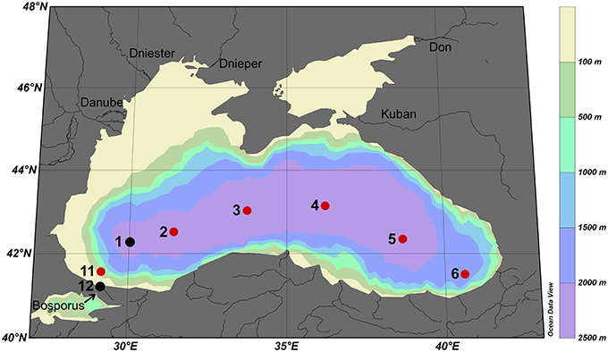
Figure 1. Cruise track of research cruise 64PE373 on the RV Pelagia in July 2013. Red dots represent normal stations with typically 6 samples taken at 10, 25, 40, 55, 70, and 85 m depth, black dots represent stations with only 1 or 2 samples taken. The five largest rivers are indicated.

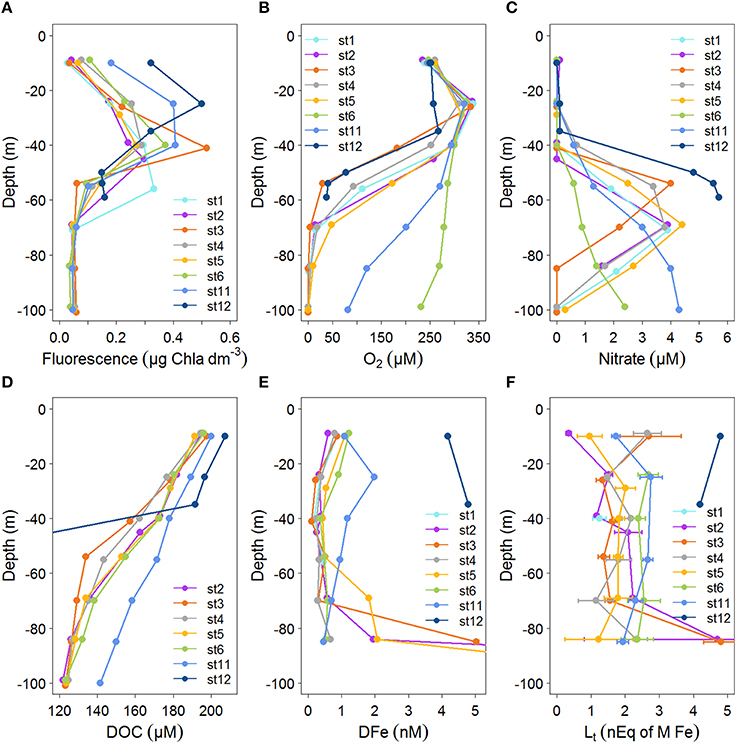
Figure 2. Profiles of concentrations with depth (0–100 m) for the stations indicated in Figure 1 for: (A) Fluorescence (μg Chlα dm⁻³) from calibrated CTD sensor data. (B) Oxygen concentration (μM) from calibrated CTD sensor data. (C) Nitrate (μM). (D) DOC (μM) from Margolin et al. (2016). DOC in station 12 at depths of 50–59 are between 78 and 90 μM. (E) Dissolved Fe (DFe, in nM), standard errors fall within the symbols (see Table 1). DFe at stations 2 and 5 at 100 m are outside the scale, DFe increased from 84 m to 100 m from 1.95 to 27.6 at station 2 and from 2.06 to 13.4 at station 5. (F) Fe-binding dissolved organic ligands, with standard errors of the fitting of the Langmuir isotherm ([L_t] in nEq of M Fe).

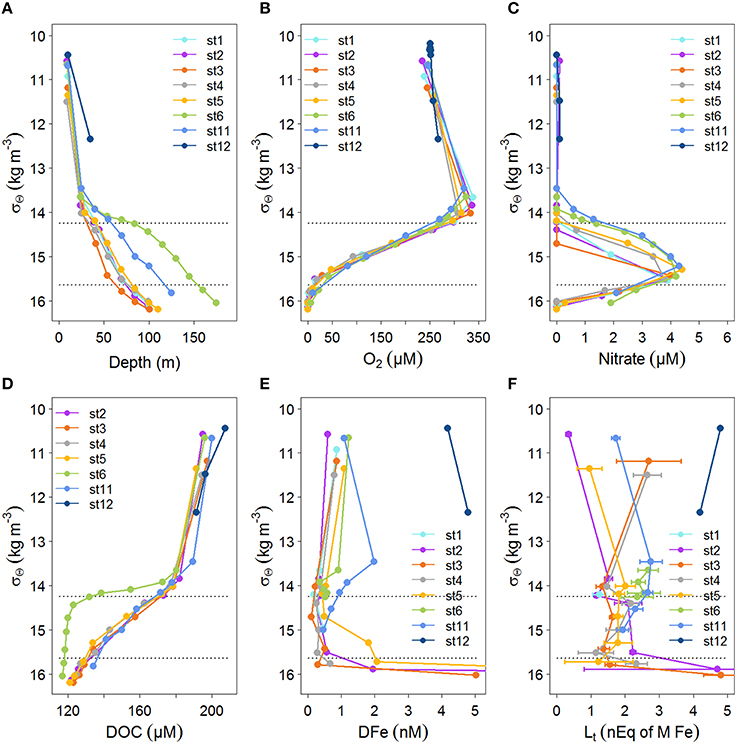
Figure 3. Profiles of concentrations with density, σ_Θ (kg m⁻³), for the stations indicated in Figure 1. The profiles are as in Figure 2 with the exception of Figure 2A, instead of fluorescence, here the relation with depth is given. If available data is given until σ_Θ = 16.2 kg m⁻³. The upper boundary of the oxycline and its lower boundary (i.e., the OL-suboxic interface) at σ_Θ = 14.25 kg m⁻³ and 15.64 kg m⁻³, respectively, are indicated by dotted lines. (A) Depth (m). (B) Oxygen concentration (μM) from calibrated CTD sensor data. (C) Nitrate (μM). (D) DOC (μM) from Margolin et al. (2016). (E) Dissolved Fe (DFe, in nM), standard errors fall within the symbols (see Table 1). DFe at stations 2 and 5 at 100 m are outside the scale, DFe increased from 84 m to 100 m from 1.95 to 27.6 at station 2 and from 2.06 to 13.4 at station 5. (F) Fe-binding dissolved organic ligands with standard errors of the fitting of the Langmuir isotherm ([L_t] in nEq of M Fe).

Samples were kept at 4°C in the dark. Fe-binding dissolved organic ligand characteristics were analyzed on board no more than 2 days after sampling. Immediately before the start of the analysis of the ligand characteristics, separate samples were taken from the un-acidified samples. These samples were acidified to pH 1.8 and measured according to the description in Section Flow Injection Analysis of DFe. Separate samples were not taken at station 11.

DOC data is from Margolin et al. (2016). Density and oxygen data were obtained from the CTD consisting of a SBE9plus underwater unit, a SBE11plusV2 deck unit, a SBE3plus thermometer, a SBE4 conductivity sensor, and a SBE43 dissolved oxygen sensor. The CTD oxygen sensor data were calibrated against discrete samples measured on board by Winkler titration (Reinthaler et al., 2006). The salinity data calculated from the CTD temperature and conductivity was calibrated against salinity measured in discrete samples analyzed on board with a Guildline 8400B Autosal using OSIL standard water batch P155. Fluorescence was measured as the beam attenuation at 660 nm using a Chelsea Aquatracka MKIII fluorometer. The fluorometer signal was calibrated against Chlorophyll a and is expressed as μg Chla dm⁻³.

Analyses

Organic Speciation of Fe

Competing Ligand Exchange—adsorptive Cathodic Stripping Voltammetry (CLE-aCSV) was performed using two setups consisting of a μAutolab potentionstat (Metrohm Autolab B.V., formerly Ecochemie, the Netherlands), a 663 VA stand with a Hg drop electrode (Metrohm) and a 778 sample processor with ancillary pumps and Dosimats (Metrohm), all controlled using a laptop running Nova 1.9 (Metrohm Autolab B.V.). The VA stands were mounted on elastic-suspended wooden platforms in aluminum frames developed at the NIOZ to minimize motion-induced noise, while electrical noise and backup power was provided by Fortress 750 UPS systems for spike suppression and noise filtering (Best Power). Sample manipulations were performed in laminar flow cabinets.

Organic complexation of Fe was determined by CLE- aCSV using 2-(2-Thiazolylazo)-p-cresol (TAC) as a measuring ligand (Croot and Johanson, 2000). The binding characteristics of Fe-binding dissolved organic ligands, the ligand concentration [L_t] (in nano-equivalents of molar Fe, nEq of M Fe) and the conditional binding strength K′ (M⁻¹), commonly expressed as log K′ were determined. The measuring ligand TAC with a final concentration of 10 μM was used, and the complex (TAC)₂-Fe was measured after equilibration (> 6 h). A borate-ammonia buffer was used to maintain pH in the samples during voltammetric scans. The buffer was adjusted to keep the pH at 8.05 in a titration subsample consisting of seawater, buffer and Fe standard additions. Buffers were prepared at NIOZ, where they were cleaned of trace metal contaminations using equilibration with MnO₂ particles after van den Berg and Kramer (1979). The increments of Fe concentrations used in the titration subsamples were 0 (2x), 0.2, 0.4, 0.6, 0.8, 1.0, 1.2, 1.5, 2, 2.5, 3, 4, 6, and 8 nM. Using a non-linear regression of the Langmuir isotherm, the ligand concentration [L_t] and the binding strength K′ (given as log K′ in Table 1A and text) were estimated. By including the sensitivity, the conversion of the recorded signal (nA) into a concentration (nM), as an unknown parameter in the non-linear regression, we allow for the possibility that the visually linear part of the titration curve is still affected by unsaturated natural ligands (Gerringa et al., 2014). The increments of Fe concentrations listed above were too low for the 10 m sample at station 3, since there [L′] was 4.6 nEq of M Fe. The estimation of [L_t] was not statistically robust, as shown by the large standard error (SE) (Table 1) (Laglera et al., 2013; Gerringa et al., 2014). To fully saturate samples, Fe additions were extended to a concentration of 12 nM in the 10, 55, and 70 m samples at station 11, while they were further extended to 20 nM in the 20 and 85 m samples, along with the 10 m sample at station 5.

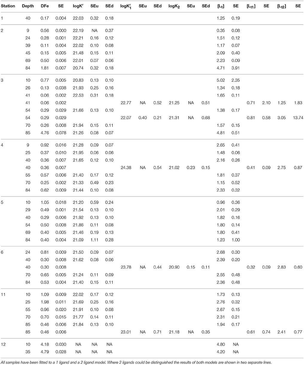
Table 1A. Dissolved Fe (DFe) in nM with standard error of the analysis, the ligand characteristics [L_t] (in nEq of M Fe) and logK′ (M⁻¹) with standard error of the fitting of the Langmuir isotherm (Gerringa et al., 2014).

Using [L_t] and K′, the concentrations of Fe bound to a natural Fe-binding ligand [FeL], the inorganic Fe [Fe′] and the natural unbound ligand [L′] were calculated using the assumption of chemical equilibrium and the mass balance DFe = [Fe³⁺](1+10^10.1+K′[L′]) and [L_t] = [FeL]+[L′], respectively by repeated calculations using Newton's algorithm (Press et al., 1986). The parameters from Liu and Millero (2002) were used and an inorganic side reaction coefficient of 10^10.1 was obtained, close to the value of 10¹⁰ determined by Hudson et al. (1992). For DFe in this calculation, the concentrations used were estimated in the separate samples taken from the un-acidified bottles (see above), except for those taken at station 11. Here, DFe concentrations that were determined in samples that were acidified immediately after collection were used. DFe obtained from the subsamples at station 1–6, were 16% lower than DFe obtained in immediately acidified samples (unpublished data), due to wall adsorption in the un-acidified sample bottles. This agrees well with Gerringa et al. (2014), who reported that DFe concentrations in samples taken from un-acidified samples from the Western Atlantic Ocean were 13% lower than in immediately acidified samples.

The ligand characteristics were calculated with two models, one assuming the presence of one ligand class and the other assuming the presence of two ligand classes (Table 1A). The two ligand model converged successfully only at a few samples.

The side reaction coefficient of the ligands (alphaFeL, given as log(alphaFeL)) was also calculated as the product of K′ and [L′]. In samples where two ligand classes could be discriminated, two values of alphaFeL were calculated: alphaFeL with the data from the one ligand model and the other with the data from the two ligand model (${\text{K}}_1^{\prime }$ and [${\text{L}}_1^{\prime }$] and ${\text{K}}_2^{\prime }$ and [${\text{L}}_2^{\prime }$]; Table 1A). AlphaFeL reflects the capacity of the dissolved organic ligands to bind with Fe, which can be seen as its ability to compete for Fe with other ligands and with adsorption sites on particles. Since the K′ at station 12 is unknown, alphaFeL cannot be calculated. AlphaFeL is a better parameter to characterize the Fe-binding dissolved organic ligands than the K′ and [L′] separately because the Langmuir equation does not treat K′ and [L′] independently from each other. If an analytical error forces an underestimation of one, the other one is automatically overestimated (Hudson et al., 2003). Moreover, [L′] is, in contrast to [L_t], independent of DFe (Thuróczy et al., 2010).

The ratio [L_t]/DFe (Table 1B) indicates the saturation of the ligands that are saturated with Fe if the ratio ≤ 1 and unsaturated when >1 (Thuróczy et al., 2010), while ignoring other competing metals (Gerringa et al., 2014; Laglera and Filella, 2015).

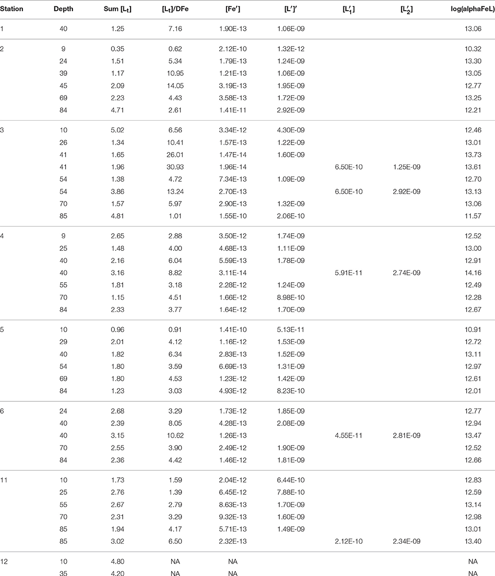
Table 1B. The sum of ligands (1 or the sum of 2 ligands concentrations, the ratio between [L_t], or the sum of both ligands, and DFe, log(alphaFeL), (for one or for two ligands), [Fe′] and [L′] (both in M), for one or for two ligand classes, [${\text{L}}_1^{\prime }$] and [${\mathrm{L}}_2^{\prime }$], were calculated from the first three variables in Table 1A (see Methods).

Flow Injection Analysis of DFe

The DFe concentrations required for data interpretation were measured at sea using an automated Flow Injection Analysis (FIA) (Klunder et al., 2011) taken from the bottles sampled for Fe complexation.

Filtered (0.2 μm, Sartorius Sartobran 300) and acidified (pH 1.8, 2 ml/L 12M Baseline grade Seastar HCl) seawater was concentrated on a column containing iminodiacetic acid (IDA). IDA only binds with transition metals and not the interfering salts. The column was then washed with ultrapure water, and eluted with 0.4 M HCl (Suprapur, Merck). After mixing with 0.6 mM luminol (Aldrich), 0.6 M hydrogen peroxide (Suprapur, Merck) and 0.96 M ammonium (Suprapur, Merck) the reaction pH was ~ 10. The resulting oxidation of luminol with peroxide was catalyzed by Fe to produce a blue light that was detected with a photon counter. The Fe concentration was calculated using a standard calibration line, where a known amount of Fe was added to seawater containing low concentrations of Fe. Using this calibration line, a number of counts per nM Fe were obtained. Samples were analyzed in triplicate and average DFe concentrations and SEs are given (Table 1). On average, the SE was 1.5%, generally being < 3% in samples with DFe concentrations higher than 0.1 nM. The average blank was determined to be at 0.033 nM, defined as the intercept of a low Fe sample loaded for 5, 10, and 20 s and was measured daily. The limit of detection of 0.019 nM was defined as 3 times the SE of the mean of the daily measured blanks (loaded for 10 s). To better understand the day-to-day variations, a duplicate sample was measured again at least 24 h later than the first measurement. The differences between these measurements were on the order of 1–20%, while the largest differences were measured in samples with low DFe concentrations. To correct for this day-to-day variation, a lab standard (sample acidified for more than 6 months) was measured daily. The consistency of the FIA system over the course of the day was verified using a drift standard. For the long-term consistency and absolute accuracy, certified SAFe and GEOTRACES reference material (Johnson et al., 2007) were measured on a regular basis.

Nutrients

Nitrate was determined on board colorimetrically (Grasshoff et al., 1983) on a Bran en Luebbe trAAcs 800 Autoanalyzer. The detection limit was 0.011 μM.

Results

Hydrography

The density structure of the Black Sea waters (as σ_Θ in kg m⁻³) is controlled by salinity resulting from the mixing between Mediterranean Sea and river waters. Temperature is less important for maintaining the basin's density structure. At the surface, temperature varies seasonally, resulting in a temperature minimum at ~50 m referred to as the cold intermediate layer (CIL). The CIL's maximum temperature boundaries are 8°C isotherms, with its core at σ_Θ≈14.6 kg m⁻³ (Konovalov and Murray, 2001; Margolin et al., 2016). Between the upper boundary of the CIL (i.e., lower boundary of the euphotic zone) and the OL-suboxic interface is the oxycline (Margolin et al., 2016), that ranged from σ_Θ = 14.25–15.64 kg/m³ (Figures 3A–F), at slightly lower densities than those found by Konovalov et al. (2001). The onset of sulfide began at σ_Θ = 16.2 kg m⁻³, again, at a slightly lower density than previously found (Konovalov and Murray, 2001). This was always below 85 m and thus, none of our samples contained sulfide.

Samples were taken at the same depths at each station, however, oxygen concentrations between stations were not consistent with respect to depth, while they were consistent with respect to σ_Θ (compare Figures 2B, 3B). Below ~50 m at the eastern and western boundaries of the Black Sea (i.e., at stations 6 and 11), oxygen was high and nitrate was low (Figures 2B,C), corresponding to deepening of the OL and suboxic zone (Figures 2B, 3A). High DOC and low DFe were also observed below 50 m at station 11 (Figures 2D,E). This is likely due to the general circulation (Kempe et al., 1990; Buesseler et al., 1994; Yemenicioglu et al., 2006). The wind-driven, counter clockwise (cyclonic) Rim Current flows along the coasts over the shelves and exchanges water between them and the central basin (Oguz et al., 1998; Oguz, 2002; Zhou et al., 2014).

The boundaries of the OL and suboxic zone followed the contours of the σ_Θ isopycnal surfaces across the basin, which was also reflected in other parameters, like DOC, nitrate, DFe (Figures 2B–D, 3B–D), salinity and sulfide (Margolin et al., 2016). In the upper 10 m, salinity ranged from a maximum of ~18.36 in the central basin to 17.17 and 17.87 at the western and eastern boundaries, respectively, with the lowest salinity near the Bosporus at station 12 (Margolin et al., 2016). Salinity generally increased sharply to a depth of 85 m, reflected in σ_Θ (Figure 3A), and gradually increased with depth below 85 m (Margolin et al., 2016).

Biogeochemistry

At the surface (~10 m), oxygen concentrations were ~240 μM at all stations, increasing to a maximum of 320–340 μM at a depth of ~25 m, with the exception of station 12 near the Bosporus (Figures 1, 2B). Below ~40 m, concentrations decreased with depth at all stations, reaching 100 μM at ~95 m at the western boundary (station 11), ~50 m in the central basin (stations 3 and 4) and ~135 m on the eastern boundary (station 6) (Figures 1, 2B). The onset of anoxia (and the redoxcline) was also shallowest in the central basin (e.g., ~80 m at stations 3 and 4) and was deeper at the basin's western and eastern boundaries (e.g., 111 and 185 m, respectively; Figures 1, 2B).

At stations 2–6 DOC decreased from >180 μM near the surface to 125–130 μM at 85 m (Figure 2D). In the upper 55 m at station 3, DOC decreased more sharply with depth than at all other stations. DOC decreased most gradually with depth at station 11 (Figure 2B). Generally, DOC profiles were similar at stations 2–6 with respect to depth (Figure 2D), while they were unique with respect to σ_Θ at station 6, having lower concentrations at σ_Θ > 14 kg m⁻³ (Figure 3D). At station 11, the depth profile of DOC deviates from other stations below ~50 m, being ~20 μM higher than other stations at these depths (Figure 2D). However, DOC at station 11 does not deviate from other stations when related to density (Figure 3D).

Nitrate is low (<0.2 μM) at all stations in the upper ~40 m, increasing to a water-column maximum of 3.9–5.7 μM between ~50 m (at stations 3 and 12) and 150 m (station 6) (Figure 2C, deep data shown in Figure 3C). This nitrate maximum approximately marks the OL-suboxic interface (Murray et al., 1995). Below this maximum in the underlying redoxcline, nitrate is removed by denitrification (Margolin et al., 2016).

The fluorescence depth distribution is generally determined by nutrient availability from below (see also Figures 2A,C), and light from above. During our study, the fluorescence maximum was between 40 and 60 m at stations 1–6 and between 20 and 30 m at stations 11 and 12 (Figures 2, 4A).

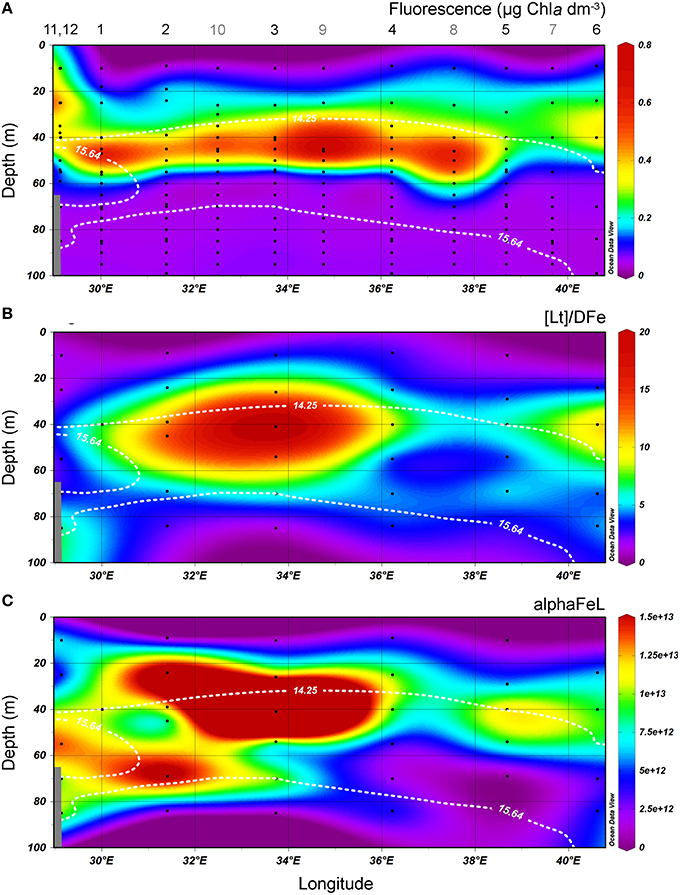
Figure 4. Transects of the cruise track of the upper 100 m from East to West. The upper boundary of the oxycline and its lower boundary (i.e., the OL-suboxic interface) at σ_Θ = 14.25 kg m⁻³ and 15.64 kg m⁻³, respectively, are indicated by white dotted lines. (A) Fluorescence (μg Chlα dm⁻³) from calibrated CTD sensor data. (B) the ratio [L_t]/DFe. (C) alphaFeL. (B,C) are both dimensionless. All data points are shown. Stations numbers are indicated above transect A. Note that more stations (indicated with gray numbers) were sampled for fluorescence. In samples where two ligands could be discriminated, the data of the two ligand model was used to calculate [L_t]/DFe and alphaFeL, [L_t] being the sum of both ligands.

DFe and Fe-Binding Dissolved Organic Ligands

DFe concentrations generally ranged from 0 to ~2 nM in the upper 85 m at stations 1–11, with one sample at station 3 having a concentration of 4.67 nM at 85 m (Figure 2E). DFe was also high at the two depths sampled near the Bosporus at station 12 (4.18 nM at 10 m and 4.80 nM at ~37 m) (Figure 2E). Concentrations near the surface at stations 2–6 ranged from 0.56 nM (at station 2) to 1.08 nM (at station 6) and decreased with depth in the upper 40 m reaching concentrations ranging between 0.06 nM (at station 3) and 0.36 nM (at station 5) at ~40 m. The concentration of DFe at station 11 was also ~1 nM (1.09 nM) near the surface, similar to stations 2–6. However, only at station 11 did concentrations first increase to 1.98 nM at 25 m followed by a decrease to concentrations of ~1 nM at 40 m. Between 40 and 85 m, concentrations increased slightly with depth at stations 2, 4, and 6 and increased considerably at stations 3 and 5. The high DFe concentrations coincided with samples taken from below the oxycline (Figure 3E). At station 11, concentrations gradually decreased to 0.46 at 85 m.

Between 40 and 85 m, concentrations tended to increase slightly with depth at stations 1, 4, and 6 and increased considerably at stations 3 and 5. The high DFe concentrations coincided with samples taken from below the oxycline (Figure 3E). At station 11, concentrations gradually decreased to 0.46 at 85 m.

[L_t] varied between 0.35 and 4.81 nEq of M Fe, with the highest concentration ranges found in the samples collected near the surface and at 85 m (Figure 2F). At station 12 near the Bosporus, high [L_t] of ~5 nEq of M Fe was found near the surface, while ~4 nEq of M Fe was found at ~37 m. At stations 1–6 and 11, concentrations generally ranged from ~1 to ~3 nEq of M Fe, with exceptions near the surface and at 85 m (Figure 2F). Near the surface at stations 2, 5, and 11, [L_t] were low (station 2 had the lowest [L_t]) and increased to a depth of 25 m, whereas at stations 3 and 4 in the center of the basin, [L_t] were elevated near the surface (~3 nEq of M Fe), decreasing to ~1 nM at 25 m. [L_t] ranged from 1 to 2.8 nEq of M Fe between ~25 and 70 m. At stations 2 and 3, [L_t] increased sharply from concentrations of ~1–2 nEq of M Fe at ~70 to concentrations of ~5 nEq of M Fe at 85 m. At station 4, [L_t] increased slightly from ~70 to 85 m, and Figure 3F shows that the increase at this depth range at stations 2–4 occurred below the oxycline. At stations 6 and 11, the deepest samples were taken above the redoxcline.

The values of logK′ were between 20.74 and 22.55 for all samples, but most of them were between 21 and 22 (25 of 34 samples) (Table 1A). Low logK′ values (<21) were found at stations 2 and 3 at 85 m and at 10 m, respectively. These low values are probably the result of an underestimation since the Langmuir equation does not treat K′ and [L′] independently from each other, as described in the Method section. If an analytical error underestimates one, the other is automatically overestimated (Hudson et al., 2003). The samples with logK′ < 21 had a relatively high [L_t] with large standard errors. High logK′ values (>22) were observed at stations 1 (10 m), 2 (4 of 6 depths) and the 40 m sample at station 3 (Table 1A).

In three samples (10 m samples at stations 2 and 5 and 85 m sample at station 3), the ligands were saturated resulting in a low ratio [L_t]/DFe (between 0.6 and 1). In all other samples [L_t]/DFe was between 1.5 and 26, with highest values typically at 40–54 m depth (Table 1B).

When the more complex two ligand model was applied, two ligand classes could be discriminated in 5 samples: station 3 at 40 and 54 m, station 4 at 40 m, station 6 at 40 m and station 11 at 85 m (Table 1A). The logK′ of the stronger ligand varied between 22.07 and 24.38, while the logK′ of the weaker ligand was between 20.9 and 21.31 (Table 1A). Only up to a few data points could be used for the calculation of the stronger ligand (2 or 3), giving results with large standard errors (Gerringa et al., 2014). [L_t] of the stronger ligand varied between 0.32 and 0.81, and [L_t] of the weaker varied between 1.25 and 3.05 nEq of M Fe.

Discussion

Possibility of Interferences by Variations in Ionic Strength and Redox Potential

The low salinity of the OL in the Black Sea (17.17–20.71) would favor higher logK′ values, since ions have higher activities at lower ionic strength. To calculate the ligand characteristics we used a binding constant between our measuring ligand TAC and Fe of logβ_Fe(TAC)2 = 22.4, as estimated by Croot and Johanson (2000). They applied their method with the estimated logβ_Fe(TAC)2 = 22.4 for S = 24–34, whereas Gerringa et al. (2007) concluded that β_Fe(TAC)2 did not change much until salinities as low as S = 10, making it an acceptable calculation for the Black Sea. A recently unpublished calibration of TAC at different salinities in melted sea ice samples by Gerringa, confirmed that the conditional binding strength β_Fe(TAC)2did not change between S = 36 and S = 10. Although the salinity did not influence β_Fe(TAC)2it might influence the binding of Fe with the naturally occurring ligands. The method of Gledhill and van den Berg (1994) using the measuring ligand 1-nitroso-2-naphtol (NN), predicted a difference of 0.3 in logβ_Fe(NN)3 between S = 17.17 and S = 34. Buck et al. (2007) used salicylaldoxime (SA) as their measuring ligand, and the conditional binding strength of logβ_Fe(SA)2 shifted by 0.11. Abualhaija and van den Berg (2014) introduced a different method using the same measuring ligand SA. Using this new SA method, Abualhaija et al. (2015) calibrated the constants of the two SA complexes, FeSA and FeSA₂, against salinity. They found a shift in ${\text{logK}}_{\text{FeSA}}^{\prime }$ of 0.06 over the above S range and a shift in logβ_Fe(SA)2 of 0.4. These calibrations of conditional binding constants of the measuring ligands NN and SA give an indication of the effect of salinity on conditional stability constants of naturally occurring ligands. The differences are not large, however, our results obtained at the relative low salinities of the OL in the Black Sea may not be comparable with results obtained at higher salinity.

Samples were not kept at the ambient redox conditions prior to analysis, however, there wasn't a noticeable offset between DFe in our samples and those measured in samples that were immediately acidified. Even in the samples with ligands that were (nearly) saturated with Fe, including the only sample taken below the oxycline (from 85 m at station 3), Fe did not precipitate in the sample bottles prior to analysis. Thus, correct determinations of DFe were obtained. Apparently even after changing the redox conditions, the ligands kept Fe in the dissolved phase.

The Ligand Characteristics logK′ and [L_t] Compared to Literature Values

Compared to the Fe ligand characteristics measured in other marine environments, the logK′ of 21–22 obtained here is relatively low, while a [L_t] of 1–2.8 nEq of M Fe is similar to values found by others in a diverse range of oceans and seas (Rue and Bruland, 1995; Cullen et al., 2006; Gledhill and Buck, 2012; Gerringa et al., 2015). Data obtained with the same method and equipment in the Western Atlantic resulted in a higher logK′ of 22.49 (standard error from mean, SE = 0.55, N = 246) and comparable average [L_t] = 1.25 (SE = 0.51, N = 246) (Gerringa et al., 2015). Kondo et al. (2007, 2012) used the same measuring ligand, but with another buffer, EPPS. They measured high logK′ values at high salinities in the coastal Sulu Sea (logK′ = 22.3–24.1, pH = 8 in Kondo et al., 2007) as well as in the open Pacific (78% of the logK′values were >22, pH = 8.1 in Kondo et al., 2012). In the present study in the Black Sea the logK′ is relatively low, although lower conditional stability constants have been reported before (Rue and Bruland, 1995; Cullen et al., 2006).

The Black Sea has a large river input, according to Margolin et al. (2016), the contribution of river water in the OL is ~50% resulting in DOC concentrations being 2.5 times higher than in the open ocean (Ducklow et al., 2007). Jones et al. (2011) showed that organic complexation is essential for the transport of Fe from the sediment and out of the estuaries. Most likely humics contribute to a large extend to the Fe-binding organic ligand pool leaving the estuaries. These humics have a relatively low logK′ according to Laglera and van den Berg (2009). They measured, using DHN as measuring ligand at pH = 8, the logK′ of fulvic and humic acids and of samples rich in humics to be between 20.6 and 21.1. These low logK′ values of humics forms an explanation of the relatively low logK′ that we found. Results from the literature on logK′ in coastal surface waters with low salinities and potentially large river influence agree well with our results, having also found lower values [20.3–22.1 in Gledhill et al. (1998), using NN as measuring ligand and pH = 6.9; 20.8–21 in Croot and Johanson (2000) using the same measuring ligand TAC and pH = 8.05 as in the present study; 20.1–21.4 in Rijkenberg et al. (2006b) using the same measuring ligand TAC and pH = 8.05, as in the present study; 20.3–21.5 in Buck and Bruland (2007) using SA as measuring ligand and pH = 8.2]. However, Buck et al. (2007), using the same method as Buck and Bruland (2007), measured higher logK′ values of 21.9–23 in estuarine waters with salinities between 1.4 and 33.9. Mahmood et al. (2015) and Abualhaija et al. (2015) (both using SA at pH = 8.1) did not find a relationship between salinity and logK′ in the Mersey estuary but [L_t] did decrease with salinity. Thus, although most coastal research resulted in relatively low logK′ values, probably due to the large input of terrigenous DOC from rivers, not all studies come to the same conclusion. Bundy et al. (2015) distinguished strong and weak ligand groups in estuarine samples. They suggested that both ligand groups consisted of humic materials and that these large molecules have different binding sites. Whether these sites are available to bind Fe depend on environmental conditions. This is an interesting view that might form the explanation for the absence of a discrete relationship between salinity and properties of the dissolved Fe binding ligands. In the Black Sea we might attribute the low the logK′ values to the nature of DOM, but we do not find a relationship between [L_t] and DOC in the Black Sea, as Wagener et al. (2008) found during a time series in the Mediterranean Sea.

Sources and Sinks of Fe and Fe-Binding Dissolved Organic Ligands

At stations 1–6, DFe was slightly elevated at the surface and high near the redoxcline. In the upper 50 m of stations 11 and 12 near the Bosporus (excluding the surface sample at station 11), DFe was higher than in the rest of the basin. Rivers are the most probable sources of DFe for these coastal stations compared to the basin interior. At station 6, DFe is higher in the upper 40 m than at stations 1–5 and 11. According to the findings of Margolin et al. (2016), the highest percentages of freshwater were found near the surface, which penetrated deeper at station 6 than at other stations. This higher percentage of freshwater at station 6 explains why the σ_Θ, oxygen and nitrate depth profiles at stations 1–5 are more similar to station 11 than station 6. This may also explain the higher DFe in the upper 40 m at station 6, when compared to stations 1–5. However, the depth profiles of DOC and [L_t] at station 6 are comparable to those at stations 2–5 (Figures 2D,F), while the DOC vs. density profile is unique (Figure 3). When comparing DOC, between stations 6 and 11, and to a lesser extent DFe, it is surprising that their distributions with respect to density are so different since both stations are located near the boundaries of the basin (Figures 1, 3D,E) and both are affected by the Rim Current. One possibility could be that processes that remove DOC are influenced more strongly or are controlled by depth rather than density. Another possible explanation for this difference is that station 6 was sampled on the eastern boundary of the Batumi eddy, which is an anti-cyclonic (clockwise), semi-permanent eddy located to the east of the Rim Current's eastern boundary (Oguz et al., 1993, 1998; Margolin et al., 2016). It is possible that the Batumi eddy is responsible for the unique DOC distribution at station 6. Influences from rivers or other anthropogenic sources are predominantly in the northwestern part of the Black Sea and are not expected to play a large role at station 6 (Borysova et al., 2005).

The anoxic water in the deep basin is known to be a source of Fe from below (Spencer and Brewer, 1971; Dyrssen and Kremling, 1990; Lewis and Landing, 1991; Tankéré et al., 2001; Yemenicioglu et al., 2006), shown here by the elevated concentrations below the oxycline (Figure 3E).

In the OL at stations 3 and 4, the Fe-binding dissolved organic ligands are higher near the surface than below, which is not observed in the other stations (Figure 2F). Apparently there is either a source of ligands in the center of the basin or greater degradation of organic ligands at the sides of the basin. Rivers as sources are expected to be more important along the coasts and especially in the north-west, where the largest rivers enter the Black Sea (Figure 1). The effect of lateral transport of organic ligands from the shelf is expected to be less in the central stations 3 and 4. Another probable explanation for a heterogeneous distribution of organic ligands might be the hydrography of the Black Sea, through the existence of the cyclonic and anticyclonic gyres and eddies (Oguz et al., 1993, 1998).

[L_t] tend to be elevated in the suboxic zone below the oxycline (Figure 3F), while no [L_t] data is available in the underlying anoxic layer. The ligands are either formed in suboxic conditions or concentrated at the redoxcline, however, with the data obtained here we cannot distinguish between these possible processes. Witter et al. (2000) found an increase in [L_t] in the oxygen minimum zone of the Arabian Sea and attributed this to biological degradation, suggesting that these ligands are breakdown products. They did not find a relationship between logK′ and the oxygen concentration. The pH influences metal speciation and it decreases with decreasing oxygen. At some of our sampled depths alkalinity and dissolved inorganic carbon (DIC) were measured, which enabled the calculation of pH. Error was estimated according to Dickson and Riley (1978) (unpublished results N. M. Clargo). In the top 10 m the pH varied between 8.15 and 8.39 (± 0.0244). At station 6 the pH remained round 8.22–8.23(± 0.0244) between 10 and 85 m. At station 5 however, the pH decreased to 7.91(± 0.0244) at 55 m (σ_Θ = 14.65 kg/m3). Hiscock and Millero (2006) found similar values, the pH was 8.3 in the upper 40 m of the Black Sea and decreased to 7.7 and 7.4 in the oxycline (σ_Θ = 14.25–15.64 kg/m³). According to Gledhill et al. (2015) a decrease in pH from 8.3 to 6.8 results in a decrease in organic complexation and an even larger decrease in inorganic complexation. The simultaneous decrease results in a decrease in organic complexation when expressed to [Fe³⁺] but in an increase when compared to [Fe′]. This might explain the high logK′ values measured in the suboxic zone of the tropical North Pacific by Hopkinson and Barbeau (2007). They attributed these relatively strong ligands either to chemical processes at low oxygen concentrations that stabilized labile Fe compounds or to production by Prochlorococcus population present in this suboxic zone. However, like we did in the Black Sea, they measured complexation at the constant pH of 8.05, and thus no information about the actual in situ changes in organic complexation could be obtained.

Complex redox cycling, such as the oxidation of reduced Fe(II) as it diffuses upwards, and the reduction of sinking Fe(III)(hydr)oxides occur near the redoxcline (Spencer and Brewer, 1971; Sorokin, 2002b; Yemenicioglu et al., 2006; Dellwig et al., 2010). [L_t] near the redoxcline will have consequences for the redox processes of Fe, since organic ligands are known to influence the oxidation and reduction of Fe (Santana-Casiano et al., 2000; Rijkenberg et al., 2006a; González et al., 2012) (in fact, this effect is used by CLE-aCSV, which change the half-wave potential of metals like Fe by complexing it to for example TAC). Increasing and decreasing oxidation rates of Fe(II) in seawater depend on the nature of the organic matter added (Santana-Casiano et al., 2000, 2010; Rijkenberg et al., 2006a; González et al., 2012). Since [L_t] tends to be saturated near the redoxcline, the net effect of these reactions likely keeps DFe in the OL and suboxic zone, decreasing the flux to the anoxic layer and retarding particle formation.

The Availability of Organically Complexed DFe

The ratio [L_t]/DFe had a maximum where ligands were relatively under saturated, corresponding to high fluorescence (Figures 2A, 4A,B). This ratio decreased due to increasing DFe concentrations above and below the fluorescence maximum (Table 1B, Figures 2A, 4A,B). In general, the log(alphaFeL) (i.e., the capacity of the dissolved organic ligands to bind with Fe) ranged from 12 to 14.16, with the two highest values (13.13 to 14.16) coinciding with the five samples in which two ligand classes were discriminated (Table 1B, Figure 4C). There were three samples outside of this range with low log(alphaFeL) values (10.31, 10.91, and 11.57) and low [L_t]/DFe ratios indicating ligands that were saturated with Fe (i.e., the 10 m samples at stations 2 and 5 and the 85 m sample at station 3). At the fluorescence maximum (40–50 m in Figures 2A, 4A), the [L_t]/DFe ratio and log(alphaFeL) tended to have their highest values (Figures 4B,C), and DFe its lowest. We found a significant correlation between log(alphaFeL) and fluorescence and between [L_t]/DFe and fluorescence (Table 2). [L_t]/DFe and log(alphaFeL) of station 11 appear to be heavily influenced by elevated DFe from the shelves. AlphaFeL is close to zero when ligands are saturated with Fe. Removing station 11 and the samples where the ligands were saturated with Fe (10 m at station 2 and 5 and 85 m at station 3) from the data does indeed result in a better relationship between fluorescence with log(alphaFeL) and with [L_t]/DFe (Table 2, Figure 5). According to our relationships only part of the Fe binding organic ligand properties can be explained by fluorescence. This means that other sources contribute to the Fe binding ligand pool. Humics from the shelves and rivers can be laterally transported as also found by others in estuaries (Laglera and van den Berg, 2009; Batchelli et al., 2010; Jones et al., 2011; Laglera et al., 2011; Abualhaija et al., 2015; Bundy et al., 2015; Mahmood et al., 2015). Arthur et al. (1994) suggested that >25% of the organic carbon in sediments was of terrestrial origin, whereas in 1996 Coble could really detect humic-like components in the Black Sea samples (Coble, 1996). Margolin et al. (2016) concluded that in our recent samples, >50% of DOC likely has a terrigenous source. Although humics are expected to be important, we cannot exclude the contribution of siderophores from bacterio-plankton (Macrellis et al., 2001; Gledhill et al., 2004; Martinez and Butler, 2007; Mawji et al., 2011) and zooplankton grazing (Sato et al., 2007; Sarthou et al., 2008) as source of ligands in the Black Sea.

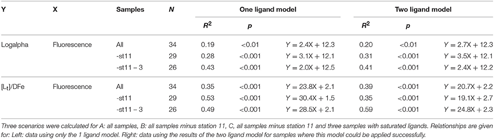
Table 2. The relationships between log(alphaFeL) and [L_t]/DFe (both dimensionless) with fluorescence ( as μg Chlα dm⁻³).

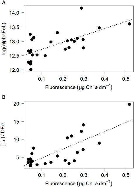
Figure 5. The ratio log(alphaFeL) (A) and [L_t]/DFe (B) vs. fluorescence (as μg Chlα dm⁻³). For those samples where two ligands could be discriminated the data of the two ligand model was used. In Table 2 three scenarios were calculated, including the relationships, p and R².

The increasing log(alphaFeL) results from an increase in [L′]. [L′] can increase due to an increase in [L_t], an accumulation of ligands by for example microbial production (Rue and Bruland, 1995; Gerringa et al., 2006; Tian et al., 2006; Buck and Bruland, 2007) or a lateral supply (Laglera and van den Berg, 2009; Batchelli et al., 2010; Jones et al., 2011; Laglera et al., 2011; Abualhaija et al., 2015; Bundy et al., 2015; Mahmood et al., 2015). Alternatively, [L′] can increase due to the biological utilization of Fe from organic Fe-complexes (decreasing [FeL] at a constant [L_t]). Here we define biological utilization of Fe as the transfer of Fe from the ligand pool to the cells without defining if the Fe is internalized or is adsorbed or bound to the outside of the cell. However, Twining et al. (2015) found that externally scavenged Fe was not a significant Fe fraction of life phytoplankton cells. Anyhow, the consequence of the biological utilization of Fe is that [L′] increases because Fe is removed from the organic ligands. In the Black Sea, the suggested biological utilization of Fe from the natural dissolved organic ligands resulted in low [Fe′] (inorganic Fe not bound by dissolved organic ligands, Table 1B).

Fe complexed by natural dissolved organic ligands is biologically available, as observed by Maldonado et al. (2001, 2005) in the Southern Ocean and sub-Antarctic waters. Maldonado et al. (2005) and Shaked et al. (2005) showed that Fe was taken up from strong Fe binding organic ligands by bacteria and phytoplankton including diatoms. Photochemistry of the Fe-complexes appeared to play a role, although according to Maldonado et al. (2005) the photolability of the ligands was not the determining factor. Shaked et al. (2005) introduced a new uptake model in which extracellular reduction at the cell wall was a necessary step in the uptake process. The reductive step theory has the advantage that it is non-specific for both the type of micro-organisms and the organic Fe-species (Shaked and Lis, 2012). However, other uptake processes exist, see references in Shaked and Lis (2012). The low [Fe′] and high [L′] that we find indicates that most ligands were not destroyed during biological utilization leaving the ligands intact for further complexation of Fe.

Acknowledging the existence of two ligand classes in five samples improves the correlation between fluorescence with log(alphaFeL) and with [L_t]/DFe even more (Figure 5, Table 2). Four out of the five samples in which two ligand classes were distinguished occurred in the fluorescence maximum. Also here it is tempting to conclude that phytoplankton produced the relative strong ligand class, as was concluded by a.o. Rue and Bruland (1995). However, another explanation might be that Fe has been utilized by phytoplankton, not only from the relatively weak Fe-binding organic ligands, but also from the relatively strong Fe-binding organic ligands. When the relatively strong Fe-binding organic ligands are unsaturated, these can be titrated with Fe during the analysis and thus can be distinguished (Gerringa et al., 2014).

Although a relationship between [L_t] and the fluorescence maximum has been observed before (Gerringa et al., 2006), this is not the case for alphaFeL. The reason that this relationship is shown so clearly here might be due to the Black Sea's inland setting and local DFe sources. DFe concentrations are relatively high especially near the redoxcline, and relatively low DFe exists at 40 m depth where the maximum fluorescence was recorded (Figures 2A,E). This contrast over a relatively shallow depth range may highlight the relationship between fluorescence with log(alphaFeL) and with [L_t]/DFe.

Conclusions

Compared with ligand characteristics from open ocean environments the logK′ of 21–22 measured in the OL of the Black Sea is relatively low. This is probably due to the more coastal sources of DOC (i.e., terrigenous origin), and is likely not because of the Black Sea's lower salinity. [L_t] of 1–2.8 nEq of M Fe is similar to the average values found in other seas and oceans.

Sampling at different redox environments where different redox processes occur, did not affect the logK′ within the detection window of our method (Apte et al., 1988; Sander et al., 2011; Gerringa et al., 2014; Laglera and Filella, 2015; Pižeta et al., 2015). In the suboxic zone DFe was higher due to an increase in solubility. Also [L_t] increased in the suboxic zone and the ligands here were saturated with Fe. Ligands were also saturated with Fe near the Bosporus and at 2 stations in the surface. Everywhere else it was the presence of unsaturated dissolved organic ligands that determined the solubility of Fe. This means that in the OL, the solubility and chemical availability of DFe is largely controlled by the dissolved organic ligands.

A significant relationship existed between the alpha coefficient of the dissolved organic ligands and fluorescence, and also between the ratio [L_t]/DFe and fluorescence. These relationships are best explained by Fe bound by dissolved organic ligands being utilized by phytoplankton.

An interesting observation was that [L_t] increased near the suboxic zone at most stations. Transport of Fe over the oxic—anoxic boundary depends strongly on redox processes and the solubility of Fe. Organic complexation of Fe, affecting Fe solubility and redox processes, can therefore play an important role in the vertical transport of Fe in the Black Sea (Santana-Casiano et al., 2010; González et al., 2012).

Author Contributions

MR, LG, and HD were responsible for the design of this research. LG, JB, PL, and AM analyzed data. LG and MR did data interpretation. The first draft of the manuscript was made by LG and MR. All other co-authors contributed considerably to make the second and third drafts. All authors agreed on the final version of this manuscript.

Conflict of Interest Statement

The authors declare that the research was conducted in the absence of any commercial or financial relationships that could be construed as a potential conflict of interest.

Acknowledgments

We thank Captain Pieter Kuijt and his crew of RV Pelagia for their hospitality and help during cruise 64PE373. We further thank everybody involved at Royal NIOZ who made this expedition possible. Jan van Ooijen measured nitrate. Sharyn Ossebaar measured hydrogen sulfide. Nikki Clargo and Lesley Salt measured oxygen for Sven Ober and Hendrik van Aken to calibrate the oxygen sensors. We thank Nikki Clargo for calculating pH values for us on a very short notice. We acknowledge the Dutch funding agency (project number: 822.01.015) of the national science foundation NWO for funding of this work as part of GEOTRACES. The data were collected within the GEOTRACES programme and can be requested at the British Ocean Data Centre (http://www.bodc.ac.uk).

References

Abualhaija, M. M., and van den Berg, C. M. G. (2014). Chemical speciation of iron in seawater using catalytic cathodic stripping voltammetry with ligand competition against salicylaldoxime. Mar. Chem. 164, 60–74. doi: 10.1016/j.marchem.2014.06.005
Abualhaija, M. M., Whitby, H., and van den Berg, C. M. (2015). Competition between copper and iron for humic ligands in estuarine waters. Mar. Chem. 172, 46–56. doi: 10.1016/j.marchem.2015.03.010
Apte, S. C., Gardner, M. J., and Ravenscroft, J. E. (1988). An evaluation of voltammetric titration procedures for the determination of trace metal complexation in natural waters by use of computer simulation. Anal. Chim. Acta 212, 1–21. doi: 10.1016/S0003-2670(00)84124-0
Arthur, M. A., Dean, W. E., Neff, E. D., Hay, B. J., King, J., and Jones, G. (1994). Varve calibrated records of carbonate and organic carbon accumulation over the last 20000 years in the Black Sea. Glob. Biogeochem. Cycl. 8, 195–217. doi: 10.1029/94GB00297
Batchelli, S., Muller, F. L. L., Chang, K. C., and Lee, C. L. (2010). Evidence for strong but dynamic iron-humic colloidal associations in humic-rich coastal waters. Environ. Sci. Technol. 44, 8485–8490. doi: 10.1021/es101081c
Bergquist, B. A., Wu, J., and Boyle, E. A. (2007). Variability in oceanic dissolved iron is dominated by the colloidal fraction. Geochim. Cosmochim. Acta 71, 2960–2974. doi: 10.1016/j.gca.2007.03.013
Borysova, O., Kondakov, A., Paleari, S., Rautalahti-Miettinen, E., Stolberg, F., and Daler, D. (2005). Eutrophication in the Black Sea Region; Impact Assessment and Causal Chain Analysis. Kalmar: University of Kalmar.
Boyd, P. W., Ibisanmi, E., Sander, S. G., Hunter, K. A., and Jackson, G. A. (2010). Remineralization of upper ocean particles: implications for iron biogeochemistry. Limnol. Oceanogr. 55, 1271–1288. doi: 10.4319/lo.2010.55.3.1271
Buck, K. N., and Bruland, K. W. (2007). The physicochemical speciation of dissolved iron in the Bering Sea, Alaska. Limnol. Oceanogr. 52, 1800–1808. doi: 10.4319/lo.2007.52.5.1800
Buck, K. N., Lohan, M. C., Berger, C. J. M., and Bruland, K. W. (2007). Dissolved iron speciation in two distinct river plumes and an estuary: implications for riverine iron supply. Limnol. Oceanogr. 52, 843–855. doi: 10.4319/lo.2007.52.2.0843
Buesseler, K. O., Livingston, H. D., Ivanov, L., and Romanov, A. (1994). Stability of the oxic-anoxic interface in the Black Sea. DSR 41, 283–296. doi: 10.1016/0967-0637(94)90004-3
Bundy, R. M., Abdulla, H. A., Hatcher, P. G., Biller, D. V., Buck, K. N., and Barbeau, K. A. (2015). Iron-binding ligands and humic substances in the San Francisco Bay estuary and estuarine-influenced shelf regions of coastal California. Mar. Chem. 173, 183–194. doi: 10.1016/j.marchem.2014.11.005
Cauwet, G., Deliat, G., Krastev, A., Shtereva, G., Becquevort, S., Lancelot, C., et al. (2002). Seasonal DOC accumulation in the Black Sea: a regional explanation for a general mechanism. Mar. Chem. 79, 193–205. doi: 10.1016/S0304-4203(02)00064-6
Coble, P. G. (1996). Characterization of marine and terrestrial DOM in seawater using excitation-emission matrix spectroscopy. Mar. Chem. 51, 325–346. doi: 10.1016/0304-4203(95)00062-3
Croot, P. L., and Johanson, M. (2000). Determination of iron speciation by cathodic stripping voltammetry in seawater using the competing ligand 2-(2-Thiazolylazo)-p-cresol (TAC). Electroanalysis 12, 565–576. doi: 10.1002/(SICI)1521-4109(200005)12:8<565::AID-ELAN565>3.0.CO;2-L
Croot, P. L., and Heller, M. I. (2012). The importance of kinetics and redox in the biogeochemical cycling of iron in the surface ocean. Front. Microbiol. 3:219. doi: 10.3389/fmicb.2012.00219
Cullen, J. T., Bergquist, B. A., and Moffett, J. W. (2006). Thermodynamic characterization of the partitioning of iron between soluble and colloidal species in the Atlantic Ocean. Mar. Chem. 98, 295–303. doi: 10.1016/j.marchem.2005.10.007
Dellwig, O., Leipe, T., März, C., Glockzin, M., Pollehne, F., Schnetger, B., et al. (2010). A new particulate Mn–Fe–P-shuttle at the redoxcline of anoxic basins. Geochim. Cosmochim. Acta 74, 7100–7115. doi: 10.1016/j.gca.2010.09.017
Dickson, A. G., and Riley, J. P. (1978). The effect of analytical error on the evaluation of the components of the aquatic carbon dioxide system. Mar. Chem. 6, 77–85. doi: 10.1016/0304-4203(78)90008-7
Ducklow, H. W., Hansell, D. A., and Morgan, J. A. (2007). Dissolved organic carbon and nitrogen in the Western Black Sea. Mar. Chem. 105, 140–150. doi: 10.1016/j.marchem.2007.01.015
Dyrssen, D., and Kremling, K. (1990). Increasing hydrogen sulfide concentration and trace metal behavior in the anoxic Baltic waters. Mar. Chem. 30, 193–204. doi: 10.1016/0304-4203(90)90070-S
Fujii, M., Rose, A. L., Omura, T., and Waite, T. D. (2010). Effect of Fe(II) and Fe(III) transformation kinetics on iron acquisition by a toxic strain of Microcystis aeruginosa. Environ. Sci. Technol. 44, 1980–1986. doi: 10.1021/es901315a
Gerringa, L. J. A., Veldhuis, M. J. W., Timmermans, K. R., Sarthou, G., and de Baar, H. J. W. (2006). Co-variance of dissolved Fe-binding ligands with biological observations in the Canary Basin. Mar. Chem. 102, 276–290. doi: 10.1016/j.marchem.2006.05.004
Gerringa, L. J. A., Rijkenberg, M. J. A., Wolterbeek, H. T., Verburg, T., Boye, M., and de Baar, H. J. W. (2007). Kinetic study reveals weak Fe-binding ligand, which affects the solubility of Fe in the Scheldt estuary. Mar. Chem. 103, 30–45. doi: 10.1016/j.marchem.2006.06.002
Gerringa, L. J. A., Rijkenberg, M. J. A., Thuróczy, C.-E., and Maas, L. R. M. (2014). A critical look at the calculation of the binding characteristics and concentration of iron complexing ligands in seawater with suggested improvements. Environ. Chem. 11, 114–136. doi: 10.1071/EN13072
Gerringa, L. J. A., Rijkenberg, M. J. A., Schoemann, V., Laan, P., and de Baar, H. J. W. (2015). Organic complexation of iron in the West Atlantic Ocean. Mar. Chem. 177, 434–446. doi: 10.1016/j.marchem.2015.04.007
Gledhill, M., and van den Berg, C. M. G. (1994). Determination of complexation of iron (III) with natural organic complexing ligands in seawater using cathodic stripping voltammetry. Mar. Chem. 47, 41–54. doi: 10.1016/0304-4203(94)90012-4
Gledhill, M., van den Berg, C. M. G., Nolting, R. F., and Timmermans, K. R. (1998). Variability in the speciation of iron in the northern North Sea. Mar. Chem. 59, 283–300. doi: 10.1016/S0304-4203(97)00097-2
Gledhill, M., Mccormack, P., Ussher, S., Achterberg, E. P., Mantoura, R. F. C., and Worsfold, P. J. (2004). Production of siderophore type chelate by mixed bacterioplankton populations in nutrient enriched seawater incubations. Mar. Chem. 88, 75–83. doi: 10.1016/j.marchem.2004.03.003
Gledhill, M., and Buck, K. N. (2012). The organic complexation of iron in the marine environment: a review. Front. Microbiol. 3:69. doi: 10.3389/fmicb.2012.00069
Gledhill, M., Achterberg, E. P., Li, K., Mohamed, K. N., and Rijkenberg, M. J. (2015). Influence of ocean acidification on the complexation of iron and copper by organic ligands in estuarine waters. Mar. Chem. 177, 421–433. doi: 10.1016/j.marchem.2015.03.016
González, A. G., Santana-Casiano, J. M., González-Dávila, M, and Pérez, N. (2012). Effect of organic exudates of Phaeodactylum tricornutum on the Fe(II) oxidation rate constant. Cienc. Mar. 38, 245−261. doi: 10.7773/cm.v38i1B.1808
Grasshoff, K., Ehrhard, M., and Kremling, K. (1983). Methods of Seawater analysis. Weinheim: Verlag Chemie GmbH. 419.
Hansell, D. A., Carlson, C. A., Repeta, D. J., and Schlizter, R. (2009). Dissolved organic matter in the ocean: a controversy stimulates new insights. Oceanography 22, 202–211. doi: 10.5670/oceanog.2009.109
Hassler, C. S., Norman, L., Mancuso, N. C. A., Clementson, L. A., Robinson, C., Schoemann, V., et al. (2015). Iron associated with exopolymeric substances is highly bioavailable to oceanic phytoplankton. Mar. Chem. 173, 136–147. doi: 10.1016/j.marchem.2014.10.002
Hiscock, W. T., and Millero, F. J. (2006). Alkalinity of the anoxic waters in the Western Black Sea. DSR II 53, 1787–1801. doi: 10.1016/j.dsr2.2006.05.020
Hopkinson, B. M., and Barbeau, K. A. (2007). Organic and redox speciation of iron in the eastern tropical North Pacific suboxic zone. Mar. Chem. 106, 2–17. doi: 10.1016/j.marchem.2006.02.008
Hudson, R. J. M., Covault, D. T., and Morel, F. M. M. (1992). Investigations of iron coordination and redox reactions in seawater using 59Fe radiometry and ion-pair solvent extraction of amphiphilic iron complexes. Mar. Chem. 38, 209–235. doi: 10.1016/0304-4203(92)90035-9
Hudson, R. J. M., Rue, E. L., and Bruland, K. W. (2003). Modeling complexometric titrations of natural water samples. Environ. Sci. Techn. 37, 1553. doi: 10.1021/es025751a
Johnson, K. S., Boyle, E., Bruland, K., Measures, C., Moffett, J., Aquilarislas, A., et al. (2007). Developing standards for dissolved iron in seawater. Eos Trans. 88, 131. doi: 10.1029/2007EO110003
Jones, M. E., Beckler, J. S., and Taillefert, M. (2011). The flux of soluble organic-iron (III) complexes from sediments represents a source of stable iron (III) to estuarine waters and to the continental shelf. Limnol. Oceanogr. 56, 1811–1823. doi: 10.4319/lo.2011.56.5.1811
Kempe, S., Liebezett, G., and Diercks, A.-R. (1990). Water balance in the Black Sea. Nature 346, 419. doi: 10.1038/346419a0
Klunder, M. B., Laan, P., Middag, R., De Baar, H. J. W., and van Ooijen, J. C. (2011). Dissolved iron in the Southern Ocean (Atlantic sector). DSR II 58, 2678–2694. doi: 10.1016/j.dsr2.2010.10.042
Kondo, Y., Takeda, S., and Furuya, K. (2007). Distribution and speciation of dissolved iron in the Sulu Sea and its adjacent waters. DSR II 54, 60–80. doi: 10.1016/j.dsr2.2006.08.019
Kondo, Y., Takeda, S., and Furuya, K. (2012). Distinct trends in dissolved Fe speciation between shallow and deep waters. Mar. Chem. 134–135, 18–28. doi: 10.1016/j.marchem.2012.03.002
Konovalov, S. K., and Murray, J. W. (2001). Variations in the chemistry of the Black Sea on a time scale of decades (1960-1995). J. Mar. Syst. 31, 217–243. doi: 10.1016/S0924-7963(01)00054-9
Konovalov, S. K., Ivanov, L. I., and Samodurov, A. S. (2001). Fluxes and budget of sulphide and ammonia in the Black Sea anoxic layer. J. Mar. Syst. 31, 203–216. doi: 10.1016/S0924-7963(01)00053-7
Kustka, A. B., Jones, B. M., Hatta, M., Field, M. P., and Milligan, A. J. (2015). The influence of iron and siderophores on eukaryotic phytoplankton growth rates and community composition in the Ross Sea. Mar. Chem. 173, 195–207. doi: 10.1016/j.marchem.2014.12.002
Laglera, L. M., Battaglia, G., and van den Berg, C. M. G. (2011). Effect of humic substances on the iron speciation in natural waters by CLE/CSV. Mar. Chem. 127, 134–143. doi: 10.1016/j.marchem.2011.09.003
Laglera, L. M., Downes, J., and Santos-Echeandía, J. (2013). Comparison and combined use of linear and non-linear fitting for the estimation of complexing parameters from metal titrations of estuarine samples by CLE/AdCSV. Mar. Chem. 155, 102–112. doi: 10.1016/j.marchem.2013.06.005
Laglera, L. M., and Filella, M. (2015). The relevance of ligand exchange kinetics in the measurement of iron speciation by CLE–AdCSV in seawater. Mar. Chem. 173, 100–113. doi: 10.1016/j.marchem.2014.09.005
Laglera, L. M., and van den Berg, C. M. G. (2009). Evidence for geochemical control of iron by humic substances in seawater. Limnol. Oceanogr. 54, 610–619. doi: 10.4319/lo.2009.54.2.0610
Lewis, B. L., and Landing, W. M. (1991). The biogeochemistry of manganese and iron in the Black Sea. DSR 38 (Suppl. 2), S773–S803. doi: 10.1016/s0198-0149(10)80009-3
Liu, X., and Millero, F. J. (2002). The solubility of iron in seawater. Mar. Chem. 77, 43–54. doi: 10.1016/S0304-4203(01)00074-3
Macrellis, H. M., Trick, C. G., Rue, E. L., Smith, G., and Bruland, K. (2001). Collection and detection of natural iron-binding ligands from seawater. Mar. Chem. 76, 175–187. doi: 10.1016/S0304-4203(01)00061-5
Mahmood, A., Abualhaija, M. M., van den Berg, C. M., and Sander, S. G. (2015). Organic speciation of dissolved iron in estuarine and coastal waters at multiple analytical windows. Mar. Chem. 177, 706–719. doi: 10.1016/j.marchem.2015.11.001
Margolin, A. R., Gerringa, L. J. A., Hansell, D. A., and Rijkenberg, M. J. A. (2016). Net removal of dissolved organic carbon in the anoxic waters of the Black Sea. Mar. Chem. 183, 13–24. doi: 10.1016/j.marchem.2016.05.003
Martinez, J. S., and Butler, A. (2007). Marine amphiphilic siderophores: marinobactin structure, uptake, and microbial partitioning. J. Inorg. Biochem. 101, 1692–1698. doi: 10.1016/j.jinorgbio.2007.07.007
Maldonado, M. T., Boyd, P. W., Strzepek, R., LaRoche, J. L., Waite, A., Croot, P. L., et al. (2001). Phytoplankton physiological responses to changing iron chemistry during a mesoscale Southern Ocean iron enrichment. Limnol. Oceanogr. 46, 1802–1808. doi: 10.4319/lo.2001.46.7.1802
Maldonado, M. T., Strzepek, R. F., Sander, S., and Boyd, P. W. (2005). Acquisition of iron bound to strong organic complexes, with different Fe binding groups and photochemical reactivities, by plankton communities in Fe-limited subantarctic waters. Glob. Biogeochem. Cycles 19, GB4S23. doi: 10.1029/2005gb002481
Mawji, E., Gledhill, M., Milton, J., Zubkov, M., Thompson, A., Wolff, G., et al. (2011). Production of siderophore type chelates in Atlantic Ocean waters enriched with different carbon and nitrogen sources. Mar. Chem. 124, 90–99. doi: 10.1016/j.marchem.2010.12.005
Murray, J. W., Codispoti, L. A., and Friederich, G. E. (1995). “Oxidation– reduction environments: the suboxic zone in the Black Sea,” in Aquatic Chemistry: Interfacial and Interspecies Processes, Vol. 224, eds C. P. Huang, C. R. O'Melia, and J. J. Morgan (Washington, DC: American Chemical Society, The Black Sea Ecology and Oceanography), 157–176. doi: 10.1021/ba-1995-0244.ch007
Nishioka, J., Takeda, S., Kondo, Y., Obata, H., Doi, T., Tsumune, D., et al. (2009). Changes in iron concentrations and bio-availability during an open-ocean mesoscale iron enrichment in the western subarctic Pacific, SEEDS II. DSR II 56, 2796–2809. doi: 10.1016/j.dsr2.2009.06.006
Oguz, T., Latun, V. S., Latif, M. A., Vladimirov, V. V., Sur, H. I., Markov, A. A., et al. (1993). Circulation in the surface and intermediate layers of the Black Sea. DSR I 40, 1597–1612. doi: 10.1016/0967-0637(93)90018-x
Oguz, T., Ivanov, L. I., and Besiktepe, S. (1998). “Circulation and hydrographic characteristics of the Black Sea during July 1992,” in Ecosystem Modeling As a Management Tool for the Black Sea. NATO Science Series, Vol. 2, eds L. I. Ivanov and T. Oguz (Dordrecht: Kluwer Academic Publishers), 69–91.
Oguz, T. (2002). Role of physical processes controlling oxycline and suboxic layer structures in the Black Sea. Glob. Biogeochem. Cycles 16, 3-1–3-13. doi: 10.1029/2001gb001465
Pakhomova, S., Vinogradova, E., Yakushev, E., Zatsepin, A., Shtereva, G., Chasovnikov, V., et al. (2014). Interannual variability of the Black Sea Proper oxygen and nutrients regime: the role of climatic and anthropogenic forcing. Est. Coast. Shelf Sci. 140, 134–145. doi: 10.1016/j.ecss.2013.10.006
Pižeta, I., Sander, S. G., Hudson, R. J. M., Baars, O., Barbeau, K. A., Buck, K. N., et al. (2015). Quantitative analysis of complexometric titration data: an intercomparison of methods for estimating models of metal complexation by mixtures of natural ligands. Mar. Chem. 173, 3–24. doi: 10.1016/j.marchem.2015.03.006
Polat, S. C., and Tuğrul, S. (1995). Nutrient and organic carbon exchanges between the Black and Marmara Seas through the Bosphorus Strait. Cont. Shelf Res. 15, 1115–1132. doi: 10.1016/0278-4343(94)00064-T
Press, W. H., Flannery, B. P., Teukolsky, S. A., and Vetterling, W. T. (1986). “Root finding and nonlinear sets of equations,” in Numerical Recipes, eds W. H. Press, S. A. Teukolsky, W. T. Vetterling, and B. P. Flannery (Cambridge: Cambridge University Press), 347–393.
Reinthaler, T., Bakker, K., Manuels, R., van Ooijen, J., and Herndl, G. J. (2006). Fully automated spectrophotometric approach to determine oxygen concentrations in seawater via continuous-flow analysis. Limnol. Oceanogr. Methods 4, 358–366. doi: 10.4319/lom.2006.4.358
Rue, E. L., and Bruland, K. W. (1995). Complexation of iron(II1) by natural organic ligands in the Central North Pacific as determined by a new competitive ligand equilibration/adsorptive cathodic stripping voltammetric method. Mar. Chem. 50, 117–138. doi: 10.1016/0304-4203(95)00031-L
Rijkenberg, M. J. A., de Baar, H. J. W., Bakker, K., Gerringa, L. J. A., Keijzer, E., Laan, M., et al. (2015).“PRISTINE”, a new high volume sampler for ultraclean sampling of trace metals and isotopes. Mar. Chem. 177, 501–509. doi: 10.1016/j.marchem.2015.07.001
Rijkenberg, M. J. A., Gerringa, L. J. A., Carolus, V. E., Velzeboer, I., and de Baar, H. J. W. (2006a). Enhancement and inhibition of iron photoreduction by individual ligands in open ocean seawater. Geochim. Cosmochim. Acta 70, 2790–2805. doi: 10.1016/j.gca.2006.03.004
Rijkenberg, M. J. A., Gerringa, L. J. A., Velzeboer, I., Timmermans, K. R., Buma, A. G. J., and de Baar, H. J. W. (2006b). Iron-binding ligands in Dutch estuaries are not affected by UV induced photochemical degradation. Mar. Chem. 100, 11–23. doi: 10.1016/j.marchem.2005.10.005
Rijkenberg, M. J. A., Gerringa, L. J. A., Timmermans, K. R., Fischer, A. C., Kroon, K. J., Buma, A. G. J., et al. (2008). Enhancement of the reactive iron pool by marine diatoms. Mar. Chem. 109, 29–44. doi: 10.1016/j.marchem.2007.12.001
Saliot, A., Parrish, C. C., Sadouni, N., Bouloubassi, I., Fillaux, J., and Cauwet, G. (2002). Transport and fate of Danube Delta terrestrial organic matter in the Northwest Black Sea mixing zone. Mar. Chem. 79, 243–259. doi: 10.1016/S0304-4203(02)00067-1
Sander, S. G., Hunter, K. A., Harms, H., and Wells, M. (2011). Numerical approach to speciation and estimation of parameters used in modeling trace metal bioavailability. Environm. Sci. Technol. 45, 6388–6395. doi: 10.1021/es200113v
Santana-Casiano, J. M., González-Dávila, M., Rodríguez, M. J., and Millero, F. J. (2000). The effect of organic compounds on the oxidation kinetics of Fe(II). Mar. Chem. 70, 211–222. doi: 10.1016/S0304-4203(00)00027-X
Santana-Casiano, J. M., Gonzalez-Davila, M., Gonzalez, A. G., and Millero, F. J. (2010). Fe(III) reduction in the presence of catechol in seawater. Aquat. Geochem. 16, 467−482. doi: 10.1007/s10498-009-9088-x
Sarthou, G., Vincent, D., Christaki, U., Obernosterer, I., Timmermans, K. R., and Brussaard, C. (2008). The fate of biogenic iron during a phytoplankton bloom induced by natural fertilisation: impact of copepod grazing. DSR II, 55, 734–751. doi: 10.1016/j.dsr2.2007.12.033
Sato, M., Takeda, S., and Furuya, K. (2007). Iron regeneration and organic iron(III)-binding ligand production during in situ zooplankton grazing experiment. Mar. Chem. 106, 471–488. doi: 10.1016/j.marchem.2007.05.001
Shaked, Y., and Lis, H. (2012). Disassembling iron availability to phytoplankton. Front. Microbiol. 3:123. doi: 10.3389/fmicb.2012.00123
Shaked, Y., Kustka, A. B., and Morel, F. M. M. (2005).A general kinetic model for iron acquisition by eukaryotic phytoplankton. Limnol. Oceanogr. 50, 872–882. doi: 10.4319/lo.2005.50.3.0872
Sorokin, Y. I. (2002a). “Hydrochemistry,” in The Black Sea: Ecology and Oceanography, ed K. Martens (Leiden: Backhuys Publishers), 181–236.
Sorokin, Y. I. (2002b). “Biogeochemistry of sulphur and redox processes,” in The Black Sea: Ecology and Oceanography, ed K. Martens (Leiden: Backhuys Publishers), 237–285.
Spencer, D. W., and Brewer, P. G. (1971). Vertical advection diffusion and redox potentials as controls on the distribution of manganese and other trace metals dissolved m waters of the Black Sea. J. Geophys. Res. 76, 5877–5892. doi: 10.1029/JC076i024p05877
Tankéré, S. P. C., Muller, F. L. L., Burton, J. D., Statham, P. J., Guieu, C., and Martin, J. M. (2001). Trace metal distributions in shelf waters of the north-western Black Sea. Cont. Res. 21, 1501–1532. doi: 10.1016/S0278-4343(01)00013-9
Taylor, G. T., Iabichella, M., Ho, T.-Y., Scranton, M. I., Thunell, R. C., Muller-Karger, F., et al. (2001). Chemoautotrophy in the redox transition zone of the Cariaco Basin: a significant midwater source of organic carbon production. Limnol. Oceanogr. 46, 148–163. doi: 10.4319/lo.2001.46.1.0148
Thuróczy, C.-E., Gerringa, L. J. A., Klunder, M. B., Middag, R., Laan, P., Timmermans, K. R., et al. (2010). Speciation of Fe in the Eastern North Atlantic Ocean. DSR I 57, 1444–1453. doi: 10.1016/j.dsr.2010.08.004
Thuróczy, C.-E., Gerringa, L. J. A., Klunder, M., Laan, P., Le Guitton, M., and de Baar, H. J. W. (2011). Distinct trends in the speciation of iron between the shelf seas and the deep basins of the Arctic Ocean. J. Geophys. Res. 116:C10009. doi: 10.1029/2010JC006835
Tian, F., Frew, R. D., Sander, S., Hunter, K. A., and Ellwood, M. J. (2006). Organic iron(III) speciation in surface transects across a frontal zone: the Chatham Rise, New Zealand. Mar. Freshw. Res. 57, 533–544. doi: 10.1071/MF05209
Twining, B. S., Rauschenberg, S., Morton, P. L., and Vogt, S. (2015). Metal contents of phytoplankton and labile particulate material in the North Atlantic Ocean. Prog. Oceanogr. 137, 261–283. doi: 10.1016/j.pocean.2015.07.001
Van Cappellen, P., and Wang, Y. (1996). Cycling of iron and manganese in surface sediments: a general theory for the coupled transport and reaction of carbon, oxygen, nitrogen, sulfur, iron, and manganese. Am. J. Sci. 296, 197–243. doi: 10.2475/ajs.296.3.197
van den Berg, C. M. G., and Kramer, J. R. (1979). Determination of complexing capacities of ligands in natural waters and conditional stability constants of the cooper complexes by means of manganese dioxide. Anal. Chim. Acta 106, 113–120. doi: 10.1016/S0003-2670(01)83711-9
Wagener, T., Pulido-Villena, E., and Guieu, C. (2008). Dust iron dissolution in seawater: results from a one-year time-series in the Mediterranean Sea. Geophys. Res. Lett. 35:L16601. doi: 10.1029/2008GL034581
Witter, A. E., Lewis, B. L., and Luther, G. W. (2000). Iron speciation in the Arabian Sea. DSR II 47, 1517–1539. doi: 10.1016/s0967-0645(99)00152-6
Yemenicioglu, S., Erdogan, S., and Tuğrul, S. (2006). Distribution of dissolved forms of iron and manganese in the Black Sea. DSR II 53, 1842–1855. doi: 10.1016/j.dsr2.2006.03.014
Keywords: GEOTRACES, Black Sea, Fe speciation, Fe-binding dissolved organic ligands, iron
Citation: Gerringa LJA, Rijkenberg MJA, Bown J, Margolin AR, Laan P and de Baar HJW (2016) Fe-Binding Dissolved Organic Ligands in the Oxic and Suboxic Waters of the Black Sea. Front. Mar. Sci. 3:84. doi: 10.3389/fmars.2016.00084
Received: 13 January 2016; Accepted: 17 May 2016;
Published: 31 May 2016.
Edited by:
Sylvia Gertrud Sander, University of Otago, New ZealandReviewed by:
Randelle M. Bundy, Woods Hole Oceanographic Institution, USALuis Miguel Laglera, Universidad Islas Baleares, Spain
Copyright © 2016 Gerringa, Rijkenberg, Bown, Margolin, Laan and de Baar. This is an open-access article distributed under the terms of the Creative Commons Attribution License (CC BY). The use, distribution or reproduction in other forums is permitted, provided the original author(s) or licensor are credited and that the original publication in this journal is cited, in accordance with accepted academic practice. No use, distribution or reproduction is permitted which does not comply with these terms.
*Correspondence: Loes J. A. Gerringa, loes.gerringa@nioz.nl