Interactive Optimization With Parallel Coordinates: Exploring Multidimensional Spaces for Decision Support
 Sébastien Cajot
 Nils Schüler
 Markus Peter
 Andreas Koch
 Francois Maréchal
- 1IPESE, Ecole Polytechnique Fédérale de Lausanne, Sion, Switzerland
- 2European Institute for Energy Research, Karlsruhe, Germany
Interactive optimization methods are particularly suited for letting human decision makers learn about a problem, while a computer learns about their preferences to generate relevant solutions. For interactive optimization methods to be adopted in practice, computational frameworks are required, which can handle and visualize many objectives simultaneously, provide optimal solutions quickly and representatively, all while remaining simple and intuitive to use and understand by practitioners. Addressing these issues, this work introduces SAGESSE (Systematic Analysis, Generation, Exploration, Steering and Synthesis Experience), a decision support methodology, which relies on interactive multiobjective optimization. Its innovative aspects reside in the combination of (i) parallel coordinates as a means to simultaneously explore and steer the underlying alternative generation process, (ii) a Sobol sequence to efficiently sample the points to explore in the objective space, and (iii) on-the-fly application of multiattribute decision analysis, cluster analysis and other data visualization techniques linked to the parallel coordinates. An illustrative example demonstrates the applicability of the methodology to a large, complex urban planning problem.
1. Introduction
Making a decision involves balancing multiple competing criteria in order to identify a most-preferred alternative. For simple, day-to-day decisions, this can usually be done by relying on intuition and common sense alone.
For larger, more complex decisions, common sense may not suffice, and multicriteria decision analysis (MCDA) can be used to formalize the problem, both improving the decision and making it more transparent (Keeney, 1982).
To make better decisions requires a clear knowledge of the available alternatives. However, research has shown that without adequate support, the identification of alternatives is difficult and often incomplete, even for experts in a field (León, 1999; Bond et al., 2008; Malczewski and Rinner, 2015). MCDA adopts two distinct perspectives on alternatives, depending on the considered branch (Cohon, 1978; Hwang and Masud, 1979). Multiattribute decision analysis (MADA) aims to help select the best alternative from a predetermined subset (Chankong and Haimes, 2008; Malczewski and Rinner, 2015). Such alternative-focused methods have the risk of omitting important alternatives and leading to suboptimal solutions (Keeney, 1992; Beach, 1993; Belton et al., 1997; Feng and Lin, 1999; Belton and Stewart, 2002; Siebert and Keeney, 2015). Multiobjective decision analysis (MODA) methods, on the other hand, systematically generate the alternatives based on the decision maker's (DM) objectives. They can thus be considered to promote value-focused thinking, because they require the DM to think about the driving values first, and consider the means to achieve them only second (Keeney, 1992).
However, solving multiobjective problems implies that, contrary to single-objective problems, not one well-defined solution is found, but a set of equally interesting Pareto optimal solutions. Such solutions cannot be improved in one objective without depreciating the value of another objective.
When considered collectively as a Pareto front, they inform about optimal tradeoffs between objectives. In order to make use of such results, some preferences must be articulated by the DM in order to identify a most satisfactory solution from the Pareto front. The articulation of preferences, consisting e.g., in acceptable ranges, tradeoff information, or relative weights of objectives, can be done in one of three ways (Hwang and Masud, 1979; Branke et al., 2008):
i. A posteriori, once all the Pareto optimal solutions have been identified. The advantage is that the decision maker has a complete overview of the available options. On the other hand, the calculation can be extremely long if the solution space is vast, the decision maker may not have the time to wait, and the process will certainly compute many wasteful solutions which are of little interest. Even if time were not an issue, the difficulty to visualize, interpret and understand the Pareto optimal results can compromise the trust from the DM, especially when more than three objectives are considered.
ii. A priori, before starting any calculations. This is the most efficient approach, as theoretically only one solution is calculated. However, it is also probably the most difficult from the decision maker's point of view, as it assumes that they are perfectly aware of their preferences and acceptable tradeoffs, and are able to formulate them precisely. In practice, when dealing with complex and interdisciplinary problems, this knowledge is generally unavailable until the solutions are calculated, and therefore the risk of reaching an infeasible or unsatisfactory solution is high (Meignan et al., 2015; Piemonti et al., 2017b).
iii. Interactively, as the optimization progresses. This is a common response to the limitations of a priori and a posteriori approaches. By involving the human decision maker directly in the search process (Kok, 1986), interactive optimization (IO) allows the user to learn from solutions as they are produced, refine their preferences, and in turn restrict the search to the most relevant areas of the solution space.
The goal of this paper is to highlight the current gaps in literature which are limiting the application of IO to large problems, and propose a novel methodology addressing these gaps.
1.1. Background of Interactive Optimization
Interactive optimization consists of four main components which are combined to form a human-computer interaction system: a user, a graphical user interface (GUI), a solution generator and an analyst (Figure 1).
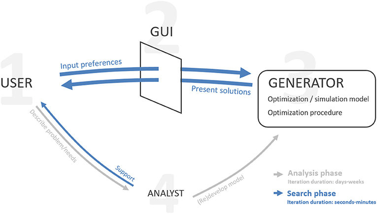
Figure 1. Main components and flows of information in interactive optimization. GUI: graphical user interface. Adapted from Spronk (1981) and Meignan et al. (2015).
During a preparatory analysis phase, the user describes the problem and criteria to the best of their knowledge, and the analyst develops the model accordingly. A feedback loop, which can overlap with the search phase, ensures the model captures the user's requirements as these evolve (Fisher, 1985). During the search phase, the user steers the generation of solutions through the GUI. Here, the role of the analyst becomes more passive (Spronk, 1981). The basic mechanism of IO consists in the oscillation between a generation phase, an exploration phase, and a steering phase. Typically, the process begins by generating and presenting one or several predetermined solutions for the user to explore. They study and compare their characteristics which are presented in the GUI, and react to them by communicating their likes or dislikes, also formalized through the GUI. These inputs are used to steer the subsequent calculations toward desired areas of the solution space. The process repeats until the user is convinced to have found the most satisfactory solution.
The main premise for human-computer interaction is that complex problems can be better solved by harnessing the respective strengths of each party (Fisher, 1985; do Nascimento and Eades, 2005; Hamel et al., 2012). The relatively superior human capabilities are in the expertise of the problem and subjective evaluations, as well as skills in strategic thinking, learning, pattern recognition and breaking rules consciously (Fisher, 1985; Klau et al., 2010; Shneiderman, 2010; Wierzbicki, 2010; Babbar-Sebens et al., 2015).
The relative strengths of the computer are in counting or combining physical quantities, storing and displaying detailed information and performing repetitive tasks rapidly and simultaneously over long periods of time (Shneiderman, 2010). In IO, the interface, or graphical user interface (GUI), allows to dialog with the user, both displaying results visually and receiving the user's preferences as inputs via mouse events or textual entries. The solution generator component consists of an optimization or simulation model describing the problem by its decision variables, objective functions and constraints, and an optimization procedure, which can be either an exact or a heuristic-based algorithm searching for solutions to the optimization problem (Collette and Siarry, 2004; Meignan et al., 2015). Some of the widely used meta-heuristic procedures include evolutionary algorithms, simulated annealing, and swarm particle optimization. Such algorithms mimic natural phenomena to explore a solution space toward optimal solutions. Unlike exact methods, they rely on stochastic exploration of solutions, searching for combinations of variables which lead to the best performance of a fitness function, or objective. This makes their implementation often simpler, but at the price of requiring many iterations to reach what is often only an approximation of the Pareto front. In the case of exact methods, such as linear (LP) or mixed-integer linear programming (MILP), the solution space is explored in a deterministic way, making the procedure overall more efficient and guaranteeing to find (at least weakly) Pareto optimal solutions. When dealing with many objectives, a parametrized scalarization function is commonly used to convert the multiple objective problem into several single objective ones, making it possible to use widely available and rapid single-objective solvers. By varying the parameters in the scalarization function, a range of Pareto optimal solutions to the initial multiobjective problem can be generated (Branke et al., 2008; Chankong and Haimes, 2008). Together, the optimizer and GUI provide an efficient and systematic framework to generate and represent a large number of Pareto optimal solutions which are most relevant to the user.
There are several compelling benefits of involving a human user in the interactive optimization process. First, the incorporation of expert knowledge, intuition and experience can compensate the unavoidable simplifications induced by the model (Meignan et al., 2015; Piemonti et al., 2017a; Liu et al., 2018). Second, computational effort is reduced by focusing on only the most promising regions of the solution space (Balling et al., 1999; do Nascimento and Eades, 2005; Liu et al., 2018). Third, the interaction process promotes trust, facilitates learning, and increases the user's confidence in the solutions and thus their likelihood of actually implementing them (Hwang and Masud, 1979; Spronk, 1981; Shin and Ravindran, 1991; Liu et al., 2018). Finally, this approach avoids the need to specify any explicit a priori preference information (Hwang and Masud, 1979; Allmendinger et al., 2016).
On the other hand, the main drawbacks are that IO methods rely on the assumptions that a human DM is available, that they are willing to devote time to the solution process, and that they are able to understand the process, inputs asked of them, and resulting outcomes (Hwang and Masud, 1979; Spronk, 1981; Collette and Siarry, 2004; Branke et al., 2008; Liu et al., 2018). This implies that developed methodologies should be both easily understandable, and able to quickly generate representative Pareto optimal solutions for the user to explore.
1.2. Related Work
1.2.1. Review of Interactive Optimization Procedures
Over the past decades, a variety of interactive optimization methods have been developed, with efforts both in improving the underlying search procedures, and interaction mechanisms. (Kok, 1986; Vanderpooten, 1989) provided an early attempt at describing and organizing IO methods. They distinguished between search-based methods, in which the DM's preference structure is supposed stable and preexisting, and learning-based methods, which promotes the discovery of preferences in problems where these are not known or difficult to express.
Many efforts have been done to review and synthesize the technical developments in the field of interactive optimization. The earlier developments of search-based methods are described by Hwang and Masud (1979), Collette and Siarry (2004), Branke et al. (2008), and Chankong and Haimes (2008). These are often classified according to the preference structures required from the DM (e.g., reference points, weights, bounds, tradeoff quantification) and the implications these have on generating Pareto optimal solutions. More recently, Meignan et al. (2015) provided an extensive review of the technical aspects of existing methods. They classified interactive methods based on the following features: the type of optimization procedure used (exact, heuristic or metaheuristic approaches), the user's contribution to the optimization process (affecting either the model or the procedure), and the characteristics of the optimization system (direct or indirect user feedback integration). Regarding optimization procedures, they found that heuristic- or metaheuristic-based approaches were predominant (25 out 32 surveyed studies), while exact approaches were the minority. A possible explanation for the popularity of metaheuristics is that in interactive methods, approximations of global optima may be good enough given the expected inaccuracies of the model. Another perspective favors however exact methods, especially for large problems with thousands of variables. Chircop and Zammit-Mangion (2013) argue that for unconstrained search spaces, stochastic search procedures will require a large number of objective function evaluations, leading to computationally intensive algorithms. Conversely, exact methods, by relying on scalarization techniques and efficient deterministic single objective approaches can quickly find optima of even large scale multiobjective problems [Branke et al., 2008; Williams, 2013; Schüler et al., 2018b, (p. 61, 64)]. This efficiency is critical because the number of solutions required to explore the solution space grows exponentially with the number of objectives (Cohon, 1978; Copado-Méndez et al., 2016). Ultimately however, the question of whether exact or heuristic methods are most efficient is debatable, and depends on the problem considered. For structured, convex, linear or quadratic programming problems, metaheuristics may not be more competitive than exact, gradient-based methods. On the other hand, because they rely on multiple solutions per iteration, evolutionary algorithms can easily benefit from parallel processing to achieve greater search efficiency. For these reasons, Branke et al. (2008, p. 64) nuance their conclusion by suggesting further research to understand the respective niches of each procedure, and to develop hybrid approaches exploiting their respective strengths.
Beyond the underlying technical aspects of interactive optimization, growing interest has been devoted to the learning opportunities which it provides. In this vein, Klau et al. (2010) argued that promoting effective interaction and learning mechanisms is more important than efficient algorithms. The reasoning is that whichever solution is produced, it ultimately is a simplification of reality which isn't directly usable. It is thus crucial that the user is able to correctly interpret and recontextualize the results. Therefore, the insights gained during the process, about the tradeoffs, synergies and feasible boundaries are eventually more useful outcomes than the solution itself.
Allmendinger et al. (2016) employ the term “navigation” to encompass not only the optimization procedure, but also the efforts made on real-time exploration of optimization results. However, among the six so-called navigation methods reviewed by Allmendinger et al. (2016), four are a posteriori methods (meaning solutions are precalculated), while only two are interactive (Korhonen and Wallenius, 1988; Miettinen et al., 2010). Their review further reveals that most of these methods tend to handle only five or less objectives, and do not consider problems with more objectives or highly uncertain conditions. They call for the development of new methods which can easily handle complex problems with many objectives, and which provide more intuitive GUIs and interaction mechanisms.
1.2.2. Interfaces for Multiobjective Interactive Optimization
The need for intuitive visualization of multiobjective optimization results and interaction with the optimizer has been recognized as a central issue (Xiao et al., 2007; Branke et al., 2008, p. 15). Meignan et al. (2015) conclude that “the development of more natural and intuitive forms of interaction with the optimization system is essential for the integration of advanced optimization methods in decision support tools.” Branke et al. (2008, p. 52) explicitly mention the importance of user-friendliness in IO as a topic for future research. This is also true for the representation of interaction with the problem, e.g., how the DM inputs their preferences (Miettinen and Kaario, 2003), and the representation of the preferences themselves (Branke et al., 2008, p. 201). Liu et al. (2018) note that despite interactive optimization being “essentially a visual analytics task,” literature is rather silent on the specifics of visuals and interaction approaches, focusing rather on optimization procedures and preference models.
Much attention has been given to advanced visualization methods for results of a posteriori multiobjective optimization methods, although their adoption in interactive methods is still low. Efforts in this area are mainly motivated by the fact that while Pareto fronts up to three objectives can be mapped in traditional planar or three dimensional representations, problems with many-objectives (i.e., more than three) are more challenging due to both the complexity of data to display, and the space required. Among the many available techniques reviewed by Branke et al. (2008) and Miettinen (2014), parallel coordinates stand out as an intuitive and scalable alternative. Introduced by Inselberg (1985) and extensively described by Inselberg (1997, 2009), parallel coordinates are similar to radar charts, except the dimensions are displayed as vertical side-by-side axes instead of radially. This allows the method to scale well to many dimensions, and facilitates the comparison of values and identification of tradeoffs, trends and clusters in the data (Shenfield et al., 2007; Akle et al., 2017). Data points are depicted as polygonal lines (or polylines), which intersect the axes at their corresponding values. The main drawbacks of parallel coordinates include cluttering of the chart when displaying many alternatives, and the impossibility to visualize all pairwise relationships between dimensions in a single chart (Heinrich and Weiskopf, 2013; Johansson and Forsell, 2016). Studies also emphasize the need for users to receive basic training to better harness parallel coordinates (Shneiderman, 1996; Wolf et al., 2009; Johansson and Forsell, 2016; Akle et al., 2017). The recent developments of interactive data visualizations have greatly alleviated these limitations by allowing the user to filter the displayed solutions, reorder axes by dragging them to explore specific pairwise relationships, or change the visual aspect of lines such as color or opacity to reveal patterns across all dimensions (Bostock et al., 2011; Fieldsend, 2016). Heinrich and Weiskopf (2013) provide an extensive review of parallel coordinates and recent developments in their interactive features.
Several studies investigated the practical applicability of parallel coordinates in the context of multiobjective optimization. Akle et al. (2017) studied their effectiveness in comparison to radar charts and combined tables for the balancing of multiple criteria and selection of preferred solutions. They found parallel coordinates to be the most effective and engaging approach for exploration, requiring less cognitive load and stress than the other charts. They also remark that parallel coordinates were the least known method, and suggest that training users could further improve the performance and usability of the approach. Stump et al. (2009) also encountered this need, and undertook a study comparing the understanding of users who never used their tool with those who had previous experience (Wolf et al., 2009). They found that novice users showed less certainty in which visualizations to use or actions to perform, and concluded that more training prior to using the tool would be necessary. They also suggest that a simplified interface with less steering and visualization features, as well as less densely packed alternatives might help users focus on relevant information and actions (Shneiderman, 2010). It has furthermore been suggested that parallel coordinates cannot display certain kinds of information and should be complemented (e.g., with spatial representations) for a more complete representation of alternatives (Xiao et al., 2007). Kok (1986), Sato et al. (2015) and Bandaru et al. (2017b) point out that when DMs only have a vague understanding of their preferences, it may be easier to specify loose ranges of preferences in the objective space, rather than exact points of preferences. The action of “brushing” available in interactive parallel coordinates charts addresses this issue. Brushing is a common action in interactive data visualization, where the user selects and highlights a subset of data, typically by dragging the pointer over the area of interest (Martin and Ward, 1995). One limitation of parallel coordinates is the visualization of Pareto fronts. It is however possible to make some interpretations, though these differ from traditional 2D plots and require familiarity with the charts. Li et al. (2017) provide some insights on how to translate Cartesian representations of Pareto fronts into parallel coordinates.
Given the widespread attention received by parallel coordinates, their adoption in the context of multiobjective optimization is not surprising. However, their use remains predominantly confined to a posteriori exploration of precalculated solutions (Bagajewicz and Cabrera, 2003; Xiao et al., 2007; Kipouros et al., 2008; Franken, 2009; Raphael, 2011; Rosenberg, 2012; Miettinen, 2014; Ashour and Kolarevic, 2015; Fieldsend, 2016; Akle et al., 2017; Bandaru et al., 2017a). Only a few studies suggested using parallel coordinates to steer the optimization procedures, but all adopt meta-heuristic approaches, limiting their applicability to smaller problems with few variables (Fleming et al., 2005; Stump et al., 2009; Sato et al., 2015; Hernández Gómez et al., 2016).
1.2.3. Overview of Existing Interactive Optimization Methods
A selected number of methods are described hereafter, outlining their responses to the issues above as well as the remaining gaps. For a more extensive overview of existing approaches, we refer to Branke et al. (2008), Meignan et al. (2015), Allmendinger et al. (2016).
The Pareto Race tool developed by Korhonen and Wallenius (1988) is considered a multiobjective linear programming navigation method (Allmendinger et al., 2016; Greco et al., 2016), and uses a visual interactive method to steer the search freely, in real-time. Much effort was dedicated to make the use of the software simple and intuitive to lay users, for example simplifying the preference input to “faster,” or “more/less of this objective,” and letting the program translate this into corresponding parameters (increments, aspiration levels, choice of goals). A later adaptation of the tool allowed handling also non-linear (i.e., quadratic-linear) problems, improving the efficiency of generating a continuous and representative portion of the Pareto front (Korhonen and Yu, 2000). The display in Pareto Race consists in bar charts reflecting the last computed solution, from which the user can request more or less of any of the objectives in the next iteration. The main limitation of this simple and intuitive method lies in the underlying iterative nature: displaying only one solution at a time prevents gaining a clear overview of all solutions and relationships between objectives. Therefore, for large problems with many objectives, the user may not be able to explore all potentially interesting solutions in a realistic amount of time. The larger the problem, the less freedom the user has to change their mind frequently (Korhonen, 1996), which limits the applicability of this method for large problems.
Another navigation method is Pareto Navigation (Monz et al., 2008), however to achieve quick and responsive interaction between the user and the tool, solutions are precalculated, while the user can then explore them, or request recombinations of existing plans which require less time to compute.
The approach developed by Miettinen and Mäkelä (2000) was allegedly the first interactive optimization method made available online. WWW-NIMBUS is a classification-based interactive multiobjective optimization method, which asks the user to classify the objectives whether they should be improved, remain identical or be relaxed. The principle is that in each iteration, the current solution should be improved according to the user's specifications. Because the process produces Pareto optimal solutions, it is necessary that at least one objective is allowed to diminish. While the original implementation was technically limited to relatively small problems, subsequent versions improved both the optimization procedures and the GUI. Hakanen et al. (2007) developed IND-NIMBUS, which included a new nonlinear solver to tackle large-scale problems such as simulated moving beds, and provided new visualizations to compare results, including 3D histograms and parallel coordinates. In A-GAMS-NIMBUS, Laukkanen et al. (2012) combined linear and nonlinear solvers, as well as a bi-level decomposition for a heat exchanger network synthesis problem in industrial processes. The ambition was to provide quick resolution of solutions, which ranged between 1 and 43 minutes per iteration.
In a separate work, Miettinen et al. (2010) proposed a reference-point interactive method, NAUTILUS, addressing two behavioral biases, namely loss aversion and anchoring effects, by encouraging the user to not interrupt the search before finding a most preferred solution. To do so, the very first solution presented to the user is a dominated one, so that each iteration does not necessarily imply sacrificing one objective in favor of another, as happens in most IO methods, where tradeoffs necessarily occur when moving from one non-dominated solution to another.
Babbar-Sebens et al. (2015) developed WRESTORE, an interactive evolutionary algorithm tool to search for preferred watershed conservation measures. The process follows a predetermined sequence of interactive “sessions” during which the user is presented with maps and quantitative indicators for different alternatives. During a session, the user either explores and learns from previously generated alternatives, is asked to rate the new alternatives with a psychometric scale (e.g., “good,” “bad,” etc.), or is supported by an automated search procedure which relieves the user from providing inputs by relying on deep learning models which mimic the user's preference model. In addition, the tool is web-based and aims to enable multiple users to explore alternatives and steer the search jointly. The visualization of the alternatives is done essentially by displaying decision variables on maps with colored layers and icons, and providing quantitative performance indicators via histogram charts. The authors concluded on the relevance of surrogate models to reduce latencies due to computational time. In their study, they report durations of around 10 min per solution using the current watershed model, and total experiment durations spanning over several hours or days. A follow-up work from Piemonti et al. (2017b), the authors studied the usability of the tool, and identified three main improvement points: (i) time dedicated to preference elicitation should be minimized to avoid user fatigue, (ii) the interface should facilitate the access and comparison of detailed information in areas of interest, and (iii) that the accumulated findings of the user should be recapitulated at the end of the process.
Stump et al. (2009) present a trade-space visualization (ATSV) tool, which aims to help designers explore the design space in search of preferred solution. This is an adaptation of the a posteriori exploration of a precalculated trade-space which (Balling et al., 2000) first coined “design by shopping.” This feature-rich tool proposes various multidimensional visualizations (scatterplots, parallel coordinates, 3D glyph plots) to explore the trade space and steer the search for new solutions. The visualization tool is coupled to a simulation model by means of an evolutionary algorithm, and the search is influenced by user inputs consisting in reference points or preference ranges. The tool provides a very flexible exploration of the design space, including infeasible and dominated solutions. While this allows a more exhaustive exploration, this necessarily is done at the expense of additional computation time, and therefore the approach is limited to computationally inexpensive simulation models, or dependent on intermediate calculation phases which rely on low-fidelity surrogate models to narrow the design space before initiating more intensive calculations.
1.3. Research Gaps and Objectives
A wide variety of preference types, procedures and interfaces for interactive methods emerge from the existing literature. However, in spite of the early efforts in developing effective search-based procedures, and the more recent efforts in making tools which enable user learning, there remains a slow progression of “application-oriented” methods, which succeed in being adopted outside of academia and for addressing real, large-scale problems (Gardiner and Vanderpooten, 1997; Allmendinger et al., 2016). Four interconnected requirements, which remain only partially achieved in existing methods, can explain this gap (Figure 2):
• First and foremost, methods must have the ability to handle many objectives, and produce many efficient alternatives reflecting the complexity of real-world problems. Xiao et al. (2007, p. 235) noted that most interactive methods still rely on a relatively limited number of solutions, possibly overlooking important Pareto optimal ones, while Allmendinger et al. (2016) found that they typically involve a limited number of objectives, rarely exceeding five. The notion of efficient, or Pareto optimal is also essential, because the goal is to focus the attention of decision makers on the most competitive solutions, and avoid wasting time on less interesting ones (Balling et al., 2000).
• The previous requirement leads to the need for methods which are capable of overcoming the associated computational burden. It is crucial that results are delivered promptly to reduce latency time for users, whose willingness to participate might otherwise be compromised (Collette and Siarry, 2004; Branke et al., 2008; Miettinen et al., 2010). This entails not only that individual solutions are rapidly calculated, but also that they efficiently provide a representative overview of the Pareto optimal front. So far, it appears the underlying trade-off with computational speed has been between either addressing only computationally inexpensive problems (or relying on low-fidelity approximations) (Stump et al., 2009), or facing longer calculation times, possibly disrupting the search and learning experience (Babbar-Sebens et al., 2015).
• Visualization approaches for multiobjective optimization results are equally important, and have been extensively reviewed by Packham et al. (2005), Miettinen (2014), and Fieldsend (2016), clarifying the advantages and limits of the available options (scatterplot matrices, spider charts, Chernoff faces, glyphs…). Among these, parallel coordinates increasingly stand out among the most efficient approaches. They are known for their intuitive representations (Packham et al., 2005; Akle et al., 2017), as well as for occupying the least amount of space per criterion, making them highly scalable to many criteria (Fleming et al., 2005). Despite these strengths, like other visualizations, parallel coordinates also suffer from a lack of readability when displaying many solutions, and the difficulty to view all pairwise relationships in a single chart. The development of interactive visualization methods such as the data-driven documents (D3) library has allowed to partly overcome these issues by filtering solutions and rearranging axes (Bostock et al., 2011; Heinrich and Weiskopf, 2013). While Inselberg (1997) provided valuable guidelines in how to effectively interpret relationships in parallel coordinates, recent studies considered more closely the interpretation of Pareto optimal solutions (Li et al., 2017; Unal et al., 2017). Furthermore, the display of quantitative criteria may not always suffice to take informed decision, and augmenting the traditional display of results with, for example, maps (Xiao et al., 2007), depictions of physical geometries (Stump et al., 2009), values of decision variables (Gardiner and Vanderpooten, 1997) or qualitative criteria (Cohon, 1978) is advised.
• Finally, a simple and intuitive interface is necessary to top the aforementioned requirements. The user must be able to not only easily understand the results, but also steer the process with minimal effort. However, the use of complex jargon, and difficult inputs are still considered barriers against a wider adoption of interactive methods in practice (Cohon, 1978; Wolf et al., 2009; Akle et al., 2017). Meignan et al. (2015), Allmendinger et al. (2016), and Branke et al. (2008, p. 52) all conclude their reviews with a call for improvements in the development of user-friendly interfaces and methods.
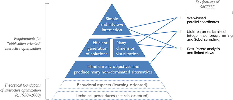
Figure 2. Summary of requirements for “application-oriented” interactive optimization methodologies. The key features from the methodology proposed in this paper (SAGESSE) and their relationship to the requirements are indicated on the right.
While the methods reviewed above address one or several of these requirements, none addresses them all simultaneously. The objectives of this paper are thus (i) to introduce a new interactive optimization methodology addressing the requirements in Figure 2, and (ii) to demonstrate its applicability to a large problem. The case-study used for the second objective relies on the multiparametric mixed integer linear programming approach described by Schüler et al. (2018b), applied to the context of urban planning.
2. Description of the SAGESSE methodology
SAGESSE – for Systematic Analysis, Generation, Exploration, Steering and Synthesis Experience – is an interactive optimization methodology designed to address the requirements summarized in Figure 2. It differs from most traditional sequential or alternating paradigms found in interactive optimization, as the steps of generation, exploration and steering blend together to form a single, continuous, interactive search process capable of tackling large problems (Figure 3). This is made possible by combining in particular three main features (Figure 2): (i) web-based parallel coordinates, as a means to simultaneously explore multiple dimensions and steer the underlying alternative generation process, (ii) deterministic optimization methods coupled with a quasi-random “Sobol” sampling method to efficiently capture large solution spaces, and (iii) on-the-fly application of Post-Pareto analysis techniques (i.e., multiattribute decision analysis and cluster analysis) as well as linked views to various representations of the solutions to support decisions. Preceding the interactive search, an analysis phase is performed by the user and the analyst to translate the constituents of the real-world problem into an optimization model (decision variables, objectives, constraints). Following the interactive search, the methodology provides a way to synthesize the gained knowledge by extracting the subset of most preferred solutions and key criteria. Overall, SAGESSE consists in an experience: a practical contact with facts, which leaves an impression on its user (Oxford, 2018). This means the user doesn't merely obtain a final solution suggested by the model, but rather acquires the knowledge and confidence of why certain solutions are preferable to them. As noted by French (1984), “a good decision aid should help the decision maker explore not just the problem, but also himself.” Finally, the confidence is reinforced by the systematic nature of the methodology, exploring the solution space with an optimization model and rigorous sampling technique, reducing the chances of missing a better alternative.
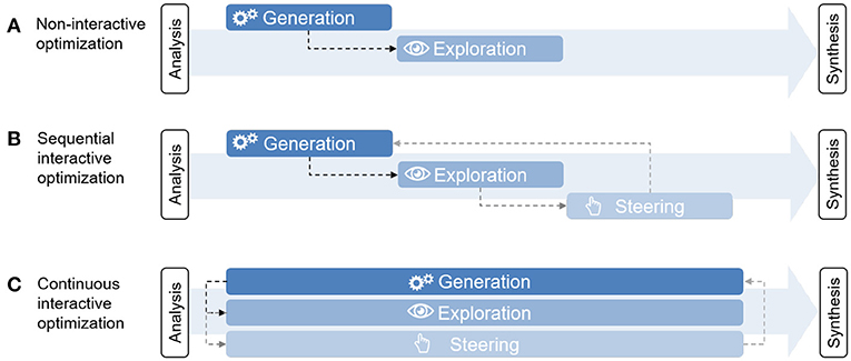
Figure 3. Novel paradigm for interactive multiobjective optimization, where generation, exploration and steering are performed continuously instead of sequentially.
2.1. Overview of Workflow
Figure 4 describes the general workflow of the methodology, which consists of six main steps. While in principle steps 1 to 5 all occur simultaneously (i.e., generation, exploration and steering tasks happen at the same time), their methodological aspects are explained hereafter sequentially.
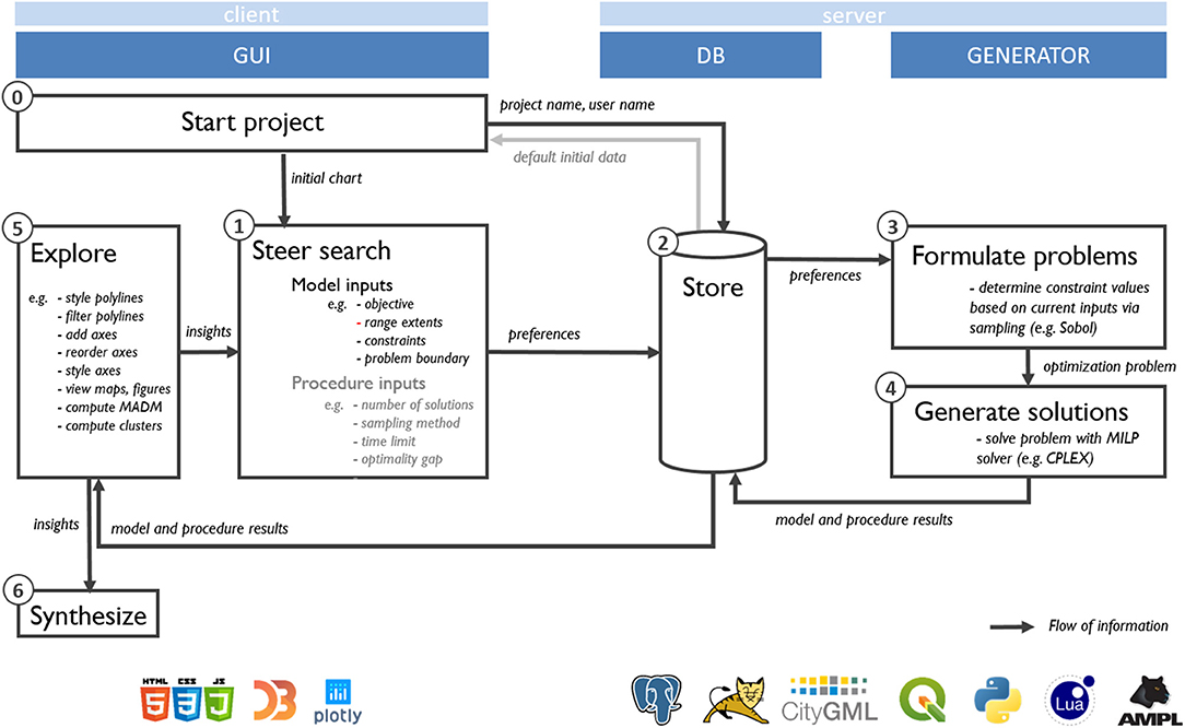
Figure 4. Overview of components, workflow and main software involved in the interactive optimization methodology and case-study. Gray text indicates optional tasks.
2.2. Starting a Project
When accessing the interface, the user can either start a new project, or reload an existing one. For a new project, by default an empty parallel coordinates chart with preselected criteria is displayed. An advantage of starting from an empty chart is that it attenuates the risk of anchoring bias, which may cause the user to fixate too soon on possibly irrelevant starting solutions, at the expense of exploring a wider variety of solutions (Miettinen et al., 2010; Meignan et al., 2015). Figure 5 shows the main components of the GUI, namely the parallel coordinates chart, and the tabs from which the user can perform and control the main SAGESSE actions.
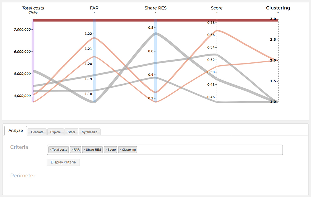
Figure 5. Snapshot of the graphical user interface demonstrating several features of the SAGESSE methodology, including axis and polyline styling, multiattribute and cluster analysis results, and the axis selection menu. The line color indicates the belonging of a line to one of the three clusters (bold axis label), while the line thickness is proportional to total costs (italic axis label).
2.3. Steering the Search
The user can influence the search in two ways: by providing inputs which influence either the optimization model, or the optimization procedure (Figure 4, Step 1). All user inputs are stored in the database, where the generator components can access them for further processing. These inputs, as well as various visual aids, constitute the available steering features, described hereafter and summarized in Table 1.
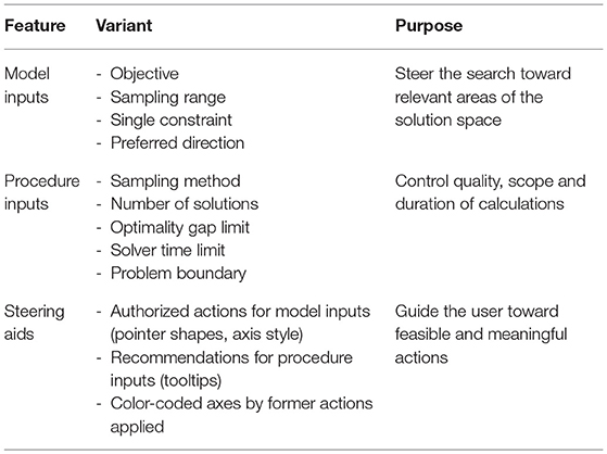
Table 1. Steering features.
2.3.1. Optimization Model Inputs
The user specifies their preferences directly on the parallel coordinates chart which is used to display the solutions. This is done by brushing the axes to be optimized or constrained (Martin and Ward, 1995).
There are three associated steering actions performed in Step 1, which will characterize the axes and the role they play in the the optimization procedure in Steps 3 and 4 (Figure 4).
• The first action consists in defining the main objective in the ϵ-constraint (epsilon-constraint) formulation described in section 2.5. Exactly one objective is specified for any new problem to be formulated. This is done by brushing the axis with the “objective” brush (colored in purple). For this action, the numeric values of the brush boundaries do not matter.
• The second action consists in marking one or several axes as single constraint so that they achieve at least (or at most, respectively) a specified value. A red brush is used for this action, and either the upper or lower bound of the brush defines the value to achieve, depending on the preferred direction of the criterion (see below).
• The third action allows to systematically vary the value of a parametrized constraint within the boundaries of a brushed range (in blue). The numeric values for these parametrized constraints are automatically determined by the chosen sampling method (cf. section 2.5), based on the requested number of solutions. While specifying single constraints denotes a “satisficing” (satisfy + suffice) behavior, which might arise if the user is certain that there is no tangible gain in achieving a value better then the specified one (Branke et al., 2008, p. 8), specifying ranges allows instead the optimization of multiple objectives (see section 2.5).
Finally, for any criterion marked as either of the above actions, its preferred direction can be specified. For example, a cost criterion's preference will be “less,” indicating that less of that criterion is preferred to more. A benefit criterion will be “more,” as more is preferred to less. Practically, “less” results in minimization for criteria brushed as objectives, and in upper constraints for criteria brushed as ranges or constraints. Conversely, “more” results in maximization for objectives, and lower constraints for ranges or constraints. Typically, default preferences are known and already included during the analysis phase for each criterion, however they can be edited by the user during the search phase, e.g., to test extreme cases.
2.3.2. Optimization Procedure Inputs
The first type of input regarding the optimization procedure is the stopping criteria for the solver, i.e., a solving time limit, and an optimality gap limit. The optimality gap is a useful feature specific to deterministic global optimization, which allows to produce solutions “that differ from the optimum by no more than a prescribed amount” (Lawler and Wood, 1966). Thus, a user can decide a priori if they would be willing to accept a solution differing by no more than e.g., 5% from the theoretical optimum, in exchange for reduced computational time. Setting looser limits, i.e., lower time or larger optimality gap limits, leads to solutions being returned earlier by the solver, but being potentially further away from the global optimum. While the first is always desirable, the latter might be acceptable in case a close approximation of the optimum solution may suffice. However it is very important to not set these limits too loosely, as solutions too far from the optimum can lead to false interpretations. It is worth emphasizing also that because the calculations are continuously performed while the user explores existing solutions, a “waiting time” of up to two minutes seems acceptable. Indeed, given the user is likely occupied interpreting the already calculated alternatives across the many criteria available, they are therefore most likely not completely idle.
A second input is the sampling method to be employed within the specified ranges, and an associated number of solutions to be sampled (see section 2.5). A third input consists in the desired scope or boundary of the problem. For example, in the case of urban planning, the perimeter to be considered in the problem can be increased or reduced.
While in principle these inputs could also be made directly via the parallel coordinates, they are specified here with buttons, forms and drop down menus. Except for the problem boundary, it should be noted that these inputs are typically predefined by the analyst, and do not require particular understanding from the user. They are rather intended for more experienced users and modelers.
2.3.3. Steering Assistance
Given the different types of content that can be displayed on the axes of the parallel coordinates chart, their typology and permitted steering actions must be clearly and intuitively conveyed to the user. The use of colored brushes, different axis styles and textual tooltips are used for this purpose. The axes can display two main types of information:
i. Methodology-specific information is displayed on axes with a dashed line style (Figure 5). They contain metadata related to the optimization procedure (e.g., iteration number, achieved optimality gap by the solver), or requested by the user in the exploration step (e.g., clustering results or aggregated score, see section 2.7).
ii. Context-specific information generated by the optimization model is displayed on axes with a continuous line style (Figure 5). As such, they can represent an objective function, a constraint, a decision variable, a model parameter or a post-computed criterion (i.e., which is calculated after all decision variables have been determined). Functions expressed as a non-linear combination of decision variables can generally not be optimized with linear solvers, and, depending on the respective formulation, can also not be constrained. They are thus restricted to being post-computed. Axes containing linear functions, model parameters or decision variables can also be brushed as single equality constraints to fix their values, as ranges in which the constraints are systematically varied, or as objectives. To guide the user in the steering process, adapted mouse pointers inform them whether or not an action is allowed on any hovered axis. Furthermore, tooltips briefly explain any forbidden action, and, if possible, how to proceed to achieve an equivalent outcome (for example by specifying a range for a criterion, whose underlying objective function implies a non-linear combination of decision variables, but which can be transformed into a linear constraint).
Another feature to assist the user in steering consists in highlighting the axes which played an active role in the optimization problem (Figure 5). This information is specific to each solution, as the role of an axis is not unique and can change as the search progresses. Thus, when hovering over a polyline, the axes which acted as objective, range or constraint in the generation of that solution are temporarily colored with the respective colors (purple, blue, and red). For example, this helps the user identify criteria which can potentially be further improved because they were so far only post-computed, and those which could be relaxed for the improvement of others.
2.4. Storing Data
A relational database is used to store both the data provided by the user in the interface (e.g., project details, raw steering preferences), and the data produced by the solution generator engine (e.g., problem formulations, solution results and related metadata). The data model for interactive optimization which was developed for the present methodology is described by Schüler et al. (2018a).
2.5. Formulating Problems
Once the user has specified the desired criteria to optimize (i.e., using objective and range brushes in Step 1), the goal is to solve the following generic multiobjective optimization problem, assuming without loss of generality all minimizing objectives (Collette and Siarry, 2004):
where the vector f(x) ∈ ℝk contains the k objective functions to minimize, g(x) ∈ ℝq are the inequality constraints, h(x) ∈ ℝr are the equality constraints, and x ∈ ℝd are the d decision variables in the feasible region S ⊂ ℝd, whose values are to be determined by the optimization procedure.
In principle, this problem could be solved with either a deterministic or a heuristic method (cf. section 1.1). However, in order to benefit from widely available and efficient optimization algorithms such as the simplex or branch-and-bound algorithms (Lawler and Wood, 1966), a deterministic approach is chosen here. To solve the problem deterministically, a scalarization function is applied to transform the multiobjective optimization problem in Equation (1) into N parametrized single-objective optimization problems which will each return a Pareto optimal solution to the original multiobjective problem (Branke et al., 2008). By varying the parameters of the scalarized function, different solutions from the Pareto front can be produced. In summary, to generate the points on a Pareto front what is needed is (i) an appropriate scalarization function, and (ii) a systematic approach to vary the parameters (Laumanns et al., 2006). The requirements for both of these aspects in the context of interactive optimization are discussed next.
2.5.1. Adopted Scalarization Function
Scalarization functions have three key requirements in the context of interactive methods (Branke et al., 2008): (i) they must have the capability of generating the entire Pareto front, while (ii) relying on intuitive input information which accurately reflect the user's preferences, and (iii) being able to quickly provide an overview of different areas on the Pareto front. Two of the most common and intuitive scalarization techniques are the weighted sum (WSM) and the ϵ-constraint methods (Mavrotas, 2009; Oberdieck and Pistikopoulos, 2016). While both are able to generate Pareto optimal solutions, the WSM only partially meets the above requirements. In the WSM, a new unique objective function is created, which consists of the weighted sum of all original k objective functions (Collette and Siarry, 2004, p. 45):
where ; n = 1, …, N, and N is the number of combinations of the weight parameters wn, i leading to Pareto optimal solutions. A first limitation of the WSM is that if the Pareto front is non-convex, the scalar function is not capable to generate solutions in that area (Branke et al., 2008; Mavrotas, 2009; Wierzbicki, 2010). Second, the WSM is biased toward extreme solutions, instead of more balance between the objectives (Branke et al., 2008; Wierzbicki, 2010). The specification of weights as inputs can have other counterintuitive and error-prone consequences on objectives, and thus be more frustrating to use for controlling the search (Cohon, 1978; Larichev et al., 1987; Tanner, 1991; Laumanns et al., 2006; Branke et al., 2008; Wierzbicki, 2010). For example, Wierzbicki (2010, p. 45) illustrates how in a three objective problem where each objective has an equal weight of 0.33, the attempt to strongly increase the first objective, slightly increase the second, and allow to reduce the third, will not be reflected accordingly in the change of weights. Indeed, in the proposed example, modifying the weights to 0.55, 0.35, and 0.1 respectively for each objective in fact only leads to an increase of the first objective, while both others are decreased. The larger the number of objectives, the greater such issues are expected to occur, and thus the more difficult it becomes for the user to determine weights which accurately reflect their preferences. Finally, the weighted sum also requires some form of normalization of incommensurable criteria toward comparable magnitudes, which can also influence the results and might require the user to specify upper and lower bounds a priori (Mavrotas, 2009).
In the ϵ-constraint method, introduced by Haimes et al. (1971), instead of optimizing all k objectives simultaneously, only one is optimized, while the other objectives are converted to parametrized inequality constraints:
where l ∈ 1, ..., k; n = 1, …N, and N is the total number of points calculated in the Pareto front, and where ϵn, j are parameters representing the upper bounds for the auxiliary objectives j ≠ l. In the original method, Nj unique upper bounds for each objective are determined within a range of interest , by incrementing by a fixed value . The minimum and maximum bounds can either be based on the expertise of the DM, or be computed by minimizing and maximizing each objective individually. The problem is solved for each unique combination of ϵn, j, i.e., for a total of N combinations, where (Chankong and Haimes, 2008, p. 285) (Figure 6A).
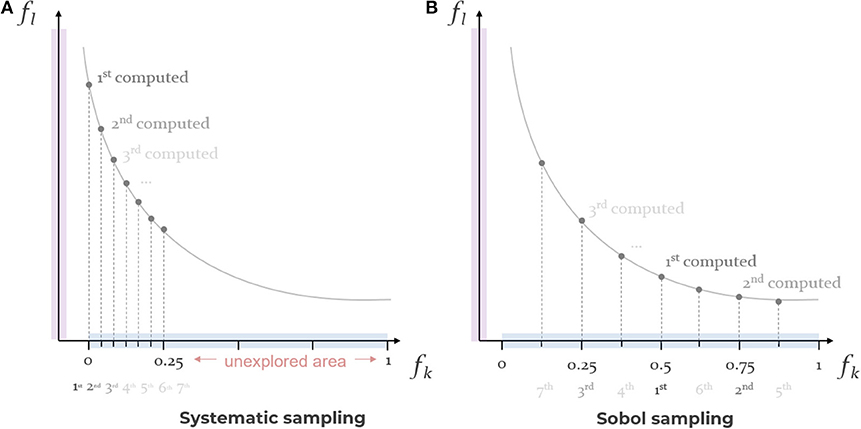
Figure 6. Schematic comparison of (A) systematic and (B) Sobol sampling for specifying constraints in an ϵ-constraint problem minimizing two objectives: state after 7 computed samples of a total of 25 requested points. Purple: main ϵ-constraint objective fl. Blue: arbitrary range of interest in the auxiliary objective fj, in which the upper bounds ϵr, j are automatically allocated by the sampling method (note: the ticks indicate the relative position of the constraints for a normalized range, and the subscripts r indicate the order in which each upper bound is used by the solver).
Conceptually, the ϵ-constraint method can be understood as the specification of a virtual grid in the objective space, and solving the single-objective optimization problem for each of the N grid points (Laumanns et al., 2006). The main advantages of the ϵ-constraint method over the weighted-sum method are that: (i) it can handle both convex and non-convex Pareto fronts (avoiding the need to evaluate the convexity of the solution space), (ii) the specification of bounds is a more intuitive and less misleading concept than setting weights (Cohon, 1978; Kok, 1986; Wierzbicki, 2010), and (iii) the variation of constraints leads to a richer and less redundant set of solutions (Branke et al., 2008; Mavrotas, 2009). For these reasons, the ϵ-constraint is adopted in the present interactive optimization methodology.
In addition to that, the original ϵ-constraint method in Equation (3) can be reformulated as a multiparametric optimization problem (Pistikopoulos et al., 2007), in which not only the upper bounds ϵn, j of the auxiliary objectives are varied, but also any other model parameter θt in the vector θ ∈ ℝm. Thus, assuming without loss of generality all minimizing functions, the nth problem being solved can be written as:
where n = 1, …N, and N is the total number of points calculated in the Pareto front. For simplicity, all parameters to be varied by a sampling scheme (regardless of whether they refer to a function fj or to a model parameter θt) are referred to as ϵn, p, where p = 1, …, P, and where, by definition, P = k − 1 + u is the total number of varied parameters. Thus, let E be the matrix of all sampled parameters in Equation (4), which contains in each row the sampled parameters of the nth problem being sent from the client to the optimization procedure:
Referring to the steering actions performed by the user and defined in section 2.3.1, the brushed objective here corresponds to fl in Equation (4), while the lower and upper bounds of brushed ranges correspond to the lower and upper bounds of the range of interest in Equation (5). It is worth noting here that for the particular case where fj(x, θ) = xd, the user can also control and vary individual decision variables directly. Finally, single constraints do not require sampling, and are thus handled separately: when brushed on an axis representing a function, a single parameter is fixed as equal to the upper value of the brush (or to the lower value of the brush for a maximizing function). Furthermore, as, from a modeling perspective, parameters do not possess any “preferred direction”, in case a single constraint brush is employed to fix their value, the lower bound of the brush is considered by default.
Despite the advantages of the ϵ-constraint method, Chankong and Haimes (2008, p. 285) noted that it can be inefficient when perturbating the values of the ϵn, p bounds in the incremental fashion described above. As such, and especially when many dimensions are involved, the generation of solutions using the ϵ-constraint method can be time-consuming and uneven across the objective space when interrupted prematurely, leading to a poor representation of the Pareto front (Collette and Siarry, 2004; Chankong and Haimes, 2008; Copado-Méndez et al., 2016). This lack of efficiency is particularly problematic in interactive methods, as the user should be presented with an overview of the Pareto optimal solutions as fast as possible in order to know which areas lead to preferred alternatives. The use of sampling techniques to facilitate and improve the determination of ϵn, p in Equation (4) is discussed next.
2.5.2. Adopted Sampling Method
Several studies have investigated ways to improve the determination of parameters in the ϵ-constraint method. For example, Chircop and Zammit-Mangion (2013) proposed an original algorithm to explore two dimensional problems more efficiently and evenly with the ϵ-constraint method, avoiding sparse Pareto fronts. However, their procedure is restricted to bi-objective problems. The use of various sampling techniques has also been studied as a means to efficiently explore a space with a minimum amount of points. Burhenne et al. (2011) compared various sampling techniques and found that the Sobol sequence (Sobol, 1967) leads to a more efficient and robust exploration of parameter spaces, and is thus recommended when sample sizes must be limited due to time or computational limitations. A Sobol sequence is a quasi-random sampling technique designed to progressively generate points as uniformly as possible in a unit hypercube (Figure 6B) (Burhenne et al., 2011). Closely related to the present approach, Copado-Méndez et al. (2016) tested the use of pseudo- and quasi-random sequences to allow the ϵ-constraint method to handle many objectives more efficiently. They obtained better quality and faster representations of Pareto optimal solutions using a combination of Sobol sequences and objective reduction techniques, compared to the standard ϵ-constraint method and other random sequences. Franken (2009) also uses a Sobol sequence approach for the exploration of promising input parameters for particle swarm optimization in parallel coordinates. However, the adoption of quasi-random sequences for real-time benefits in interactive optimization has not been tried. This approach – rather than a regular systematic sampling typically adopted in the ϵ-constraint method – is particularly relevant when dealing with interactive methods, as the order with which the solutions are explored is critical when the user's time is limited. Furthermore, the Sobol sequence greatly removes a burden from the user, who must only specify loose ranges of approximate preference or interest, and the sequence automatically takes care of determining the constraints in the next most efficient location of the solution space.
In SAGESSE, the quasi-random Sobol sampling method (Sobol, 1967) is therefore adopted and can be selected to vary the parameters in Equation (5), ensuring a quick and efficient exploration of the entire space with a minimum amount of solutions (Figure 6B).
With the Sobol sampling approach, the user specifies a number of solutions N, and the corresponding parameters in E are computed as:
where sn, p is an element in the matrix SN×P, whose rows contain the Sobol sequence of N coordinates in a P-dimensional unit hypercube. Various computer-based Sobol sequence generators have been developed and implemented to compute the elements of SN×P. Here, a Python implementation based on Bratley and Fox (1988) was used, allowing the generation of sequences including up to 40 dimensions (Naught101, 2018). Other generators could increase this number, e.g., allowing sequences for up to 1111 dimensions (Joe and Kuo, 2003). As illustration, the numeric values sampled with the Sobol approach for N = 5 points and P = 3 parameters in ranges [0, 1] are provided in Esob, Equation (7). This choice of range further implies that in this example, the coordinates of the parameters are in fact identical to those of the Sobol sequence in a unit hypercube:
Alternatively, a standard systematic sampling method can also be used (Gilbert, 1987), which can in some cases be preferred to the Sobol sampling method. With systematic sampling, the space is systematically explored by dividing the sampled dimensions into regular intervals. An important drawback from this sampling method is that it can lead to misleading or biased insights if the sampled solution space contains “unsuspected periodicities” (Gilbert, 1987). In addition, it is less convenient for real time optimization because of its slower progression throughout the solution space (Figure 6A). Nevertheless, this sampling technique can provide more control to the user than the Sobol approach. For example, it can be used to perform a systematic sensitivity analysis on the parameters in Equation (4), by systematically combining specific values on different axes. Unlike for the Sobol sequence, in this approach, the total number of sampled points is given implicitly by , where Np is the number of requested points in the range of interest of each dimension.
Therefore, each dimension thus contains Np unique values to sample, computed as:
where is the increment between each ϵn′, p. The corresponding matrix Esys resulting from systematic sampling is then populated by combining all parameter values in the following order:
As an example, for three dimensions sampled with systematic sampling between [0, 1] and for N1 = 3, N2 = 2, N3 = 2, the resulting matrix of varied parameters is:
2.6. Generating Solutions
In this step, the single-objective optimization problems formulated based on Equation (4) are solved. In particular, the solver receives from the client the main objective to optimize, as well as the values for all specified parameters contained in EN×P. As long as the user has not specified new objectives on the parallel coordinates chart, the generation process continues to add solutions in the current ranges, taking as inputs the rows of EN×P one after another. As soon as a change in objectives occurs, the solver interrupts the current sampling sequence and starts again with the newly provided objective and EN×P.
2.7. Exploring Solutions
The purpose of exploration is for the user to learn about tradeoffs and synergies between the solutions, and develop their confidence in what qualifies a good solution. The interface should offer a positive and intuitive experience, respecting the information-seeking mantra “overview, filter, details on demand” (Shneiderman, 1996). Parallel coordinates provide a basis for this mantra (Heinrich and Weiskopf, 2013), allowing the user to develop a feeling for achievable values in competing objectives, and understand the reasons preventing the achievement of goals. The available functionalities supporting exploration are summarized in Table 2 and described below, organized according to their main purpose (i.e., overview, filter or details).
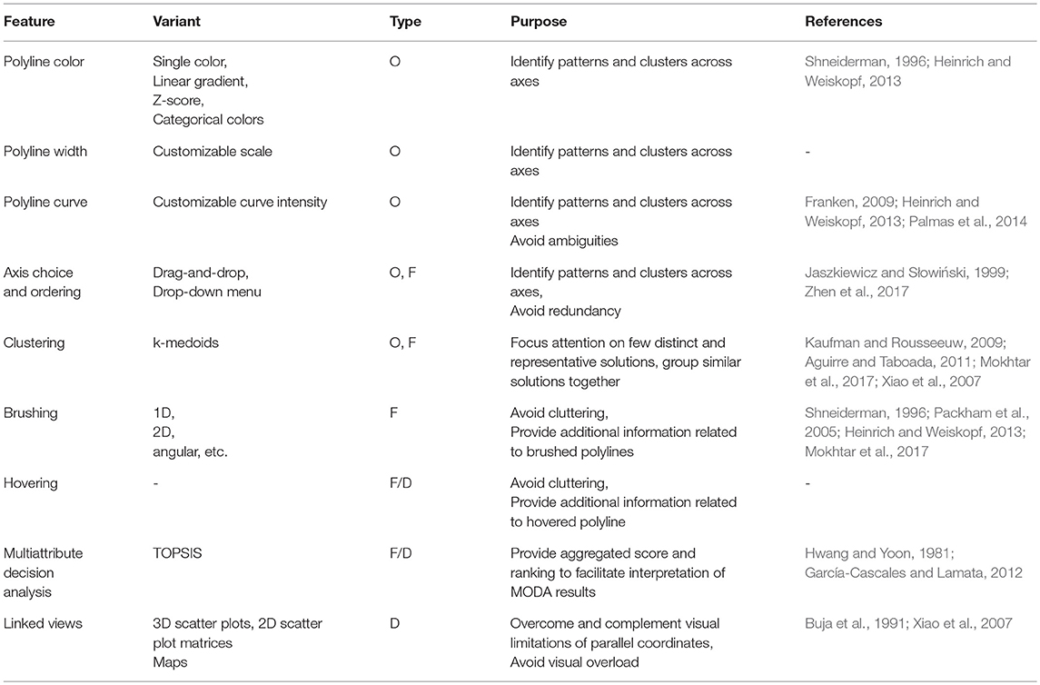
Table 2. Adopted exploration features related to the parallel coordinates interface, classified by type (O: overview, F: filter, D: details on demand).
2.7.1. Overview of Relationships Between Criteria
The parallel coordinates reveal tradeoffs (or negative correlations) between two axes as crossing lines, and synergies (or positive correlations) non-crossing lines (Inselberg, 1997; Li et al., 2017). Because the chart can only show such patterns for pairs of adjacent axes, two approaches are available to explore more relationships. First, the implementation of the chart (which relies on the data driven documents (D3) library Bostock et al., 2011; Chang, 2012) allows to dynamically drag-and-drop axes in various positions, making it possible to quickly investigate specific pairs on demand. Second, different visual encodings for the polylines can be used to emphasize various aspects of the data (Cleveland and McGill, 1985). In addition to their vertical position along each axis, properties such as color, width, line style, transparency, animation etc. can be mapped to polylines to reflect the values of a criterion. Here, color and width are used to reveal the relationships between the criterion being mapped with respect to all other axes. This allows for example to highlight high (respectively low) performing solutions, as well as clusters of solutions on any given axis. The available coloring options include linear bi- or multi-color gradients (each color shade indicates increasing values), Z-score gradient (indicating the deviation from the mean value) and categorical (assigning a unique color to each value). The line width property can be assigned to an other criterion, so that high polylines with high values are thicker than those with low values. Another way to improve readability and identify patterns and clusters is by using curves instead of lines. The user can adjust the intensity of the curvature of polylines in order to balance the readability of correlations (most readable with straight lines), and of overlapping lines and clusters (most readable with curves) (Heinrich and Weiskopf, 2013).
2.7.2. Filtering Solutions and Criteria
The user can filter the polylines to display only those of interest by “brushing” the desired axes (Heinrich and Weiskopf, 2013; Bandaru et al., 2017b). The ability to display only the solutions which satisfy desired values on the different axes is a common response to the problem of cluttering, which causes parallel coordinates to become unreadable when too many lines are present (Johansson and Forsell, 2016; Li et al., 2017). Various brushing options are available (Heinrich and Weiskopf, 2013), including a normal one-dimensional brush (defining upper and lower bounds on an axis), multiple one-dimensional brushes (to select several distinct portions on an axis), an angular brush to filter solutions according to their slope (i.e., correlation) between two axes, or two-dimensional brushes which allows the selection of solutions based on their path between two axes. Additional information can be computed for the brushed subset of polylines, such as clustering or multiattribute decision analysis. Related to brushing is the action of hovering a polyline with the pointer, which highlights it across the chart, and displays additional information (e.g., its exact numeric values for the different visible axes, information not currently displayed on the axes, or information regarding how the polyline was generated, cf. section 2.3.3). Hovering is also a way to access information in linked views, such as a graphical representation of the solution.
Another way to filter the displayed information concerns the visible axes representing the criteria. While parallel coordinates scale well to large numbers of criteria (Inselberg, 2009), in practice, working simultaneously with up to “seven plus or minus two” axes is advised to account for the user's cognitive ability (Miller, 1956). French (1984) argue that in the case of multicriteria decision analysis, this number may already be too large for simultaneous consideration. Because the relative importance of criteria in the decision process is not necessarily known in advance, and might change as new knowledge is discovered, the user must be able to access and dismiss axes in real-time. For this purpose, a drop-down menu allows to type or scroll for other criteria, and easily dismiss currently visible ones. This allows to compose new charts on-the-fly which reflect the most relevant information to the user at a given point. In the experience of the authors, the act of including criteria incrementally facilitates the consideration of even over seven axes, because the complexity gradually builds up in a structured way.
2.7.3. Filtering Representative Solutions With Clustering
The use of clustering techniques is a common approach to help make the selection of solution from a large Pareto optimal set more manageable (Aguirre and Taboada, 2011; Zio and Bazzo, 2012; Chaudhari et al., 2013). Clustering aims to group objects with similar characteristics into distinct partitions, or clusters. Practically, an algorithm seeks configurations for which “objects of the same cluster should be close or related to each other, whereas objects of different clusters should be far apart or very different” (Kaufman and Rousseeuw, 2009). A popular k-medoids technique called partitioning around medoids (PAM) is adopted here (Kaufman and Rousseeuw, 2009, p. 68). Unlike the related k-means technique which computes k virtual cluster centroids, k-medoids directly determines the most representative solutions from the existing data set (Park and Jun, 2009). While this increases computational effort, it reduces its sensitivity to outliers. Furthermore, the additional computational effort is justified in the case of interactive optimization for decision support, as it allows to focus the attention of the user on existing representative solutions, instead of virtual points which may not actually be feasible. Another main limitation of both k-means and k-medoids is the need to input a number of clusters a priori (Aguirre and Taboada, 2011). While various quality indices could be applied to assess the quality of the clusters (Goy et al., 2017), the direct feedback from the graphical display in parallel coordinates and 3D scatter plots lets the user easily explore the effect of various inputs on the final clusters (Kaufman and Rousseeuw, 2009, p. 37). The inputs consist in both the number of clusters k (specified by the user in the GUI) as well as the initial seed medoids which are chosen randomly by the algorithm from the solution set each time it is executed.
2.7.4. Filtering Solutions With Multiattribute Decision Analysis Score
When many solutions are compared across many dimensions, it can become overwhelming to distinguish which stand out overall. Psychological studies have emphasized the limited ability of human decision makers in balancing multiple conflicting criteria, even between a limited number of alternatives (French, 1984; Larichev et al., 1987; Jaszkiewicz and Słowiński, 1999). Here an aggregative multiattribute decision analysis (MADA) method is proposed to facilitate this task, by revealing the best rank or score of each alternative relative to the others (Cajot et al., 2017a). Each solution is attributed a score that is displayed as an additional axis in the parallel coordinates, and that is used as additional decision criterion.
As pointed out in the introduction (Hwang and Masud, 1979), multiobjective decision analysis (MODA) methods are designed for the generation of alternatives, while the strength of MADA lies in the evaluation and comparison of predetermined alternatives. Many methods could be adopted, and there is a wide body of literature comparing the similarities, pros and cons of these methods (Zanakis et al., 1998; Cajot et al., 2017a). The often implicit assumption with most MADA methods is that the criteria can compensate each other. While the combined strength of interactive multiobjective optimization and parallel coordinates precisely is to avoid the need to aggregate the different incommensurable criteria, providing the user with a simplified aggregated metric can nevertheless provide useful and reassuring support to make sense of the data. The resulting score is not intended to replace the DM's decision, but rather to focus their attention on a limited number of alternatives, and stimulate questions and learning (e.g., discovering what characterizes a top- or low-ranked alternative). As reviewed in Cajot et al. (2017a), the application of MADA as a way to support decisions on precalculated non-dominated sets generated with MODA is fairly common (e.g., Aydin et al., 2014; Ribau et al., 2015; Fonseca et al., 2016; Carli et al., 2017). However, these applications are typically performed a posteriori. Here, the feedback from the MADA score provides direct insights which the user can use to steer the search with MODA.
To avoid burdening the user with further methodological aspects, the Technique for Order of Preference by Similarity to Ideal Solution (TOPSIS) method is adopted for its most intuitive and understandable principle, limited need for inputs and ability to handle many criteria and solutions (Zanakis et al., 1998; Cajot et al., 2017a). The method ranks each alternative according to its proximity to an ideal solution—which would present the best value in every criterion—and respectively according to its distance from a negative ideal solution—which would present all worst values (Hwang and Yoon, 1981). The final score provided by TOPSIS is a relative closeness metric between 0 and 1, where higher scores reflect higher proximity to the positive ideal solution.
Two methodological aspects must be in particular considered in the TOPSIS method, namely the normalization of data, and the choice of ideal solutions.
First, to account for different scales in the criteria, values must be normalized for comparability (Kaufman and Rousseeuw, 2009). Two linear scale normalization methods are implemented here to handle various cases: the “max” and the “max-min” variants (Chakraborty and Yeh, 2009). The normalized values obtained with the “max” variant are . This method is advocated by García-Cascales and Lamata (2012), as it reduces the consequences of rank reversal. However, in situations where the spread of values is not consistent across criteria, this normalization tends to neglect the importance of criteria with more compact values. In case the criterion is sensitive to such small changes, these should be accounted for in the TOPSIS score. Thus, to avoid this bias, the “max-min” variant distributes all values between 0 and 1, providing not only comparable magnitudes between criteria, but also comparable spread (Chakraborty and Yeh, 2009). With this variant, the normalized values are calculated as . At the expense of being more sensitive to rank reversal, this method more accurately accounts for criteria with small spreads.
Regarding the choice of ideal solutions, while the original TOPSIS methods computes them relatively to the studied data, García-Cascales and Lamata (2012) propose the adoption of absolute positive and negative ideal points, either defined by the user or by context-specific rules. Here, the relative approach is preferred, in order to avoid asking the user for additional information, especially because of the possibly large number of criteria. They may however choose to apply the method on all computed solutions, or just a subset, for example for comparing only solutions selected in the comparer dashboard (cf. section 2.8). If the user wishes to benefit from more reliable and consistent MADA results not subject to rank-reversal, they can manually provide reasonable upper and lower bounds for each criterion, and use those absolute values instead. As noted by Wierzbicki (2010, p. 51), there are no fundamental reasons to restrict such analyses to the ranked alternatives, and using more information (e.g., absolute values if known, or historical data), or less (e.g., limiting the definition of ideals only through non-dominated solutions) can affect the strictness of the ratings. They can also give higher weights to criteria to better reflect their subjective preferences, though again to reduce the need for inputs, equal weights are assumed by default. As illustrated in Figure 9, the scores provided by the TOPSIS method easily reveal the solutions which perform best, i.e., which have both high values in criteria to maximize, and low values in the criteria to minimize.
2.7.5. Details on Demand: Linking Views to Parallel Coordinates
In some cases, the content and format of parallel coordinates is not sufficient or adapted to convey certain types of information. Xiao et al. (2007) highlight in particular the need to complement parallel coordinates visualizations with maps, while (Stump et al., 2009) suggest displaying physical geometries of generated designs - not just the design variables and performance metrics. Furthermore, Cohon (1978) noted that the communication of qualitative concepts such as aesthetics may be difficult for analysts to handle, although desirable for decision makers. Closely related is the importance to also communicate the decision variables, when requested, because in some cases the objectives and criteria alone may not provide all the necessary information to decide (Gardiner and Vanderpooten, 1997, p. 296, shenfield2007).
To address these gaps, two features are implemented. The first allows to visualize all (or subsets of) solutions in interactive 2D scatter plot matrices and 3D scatter plots (Plotly-Technologies-Inc., 2015). While these are restricted to a limited number of dimensions, they offer a more direct and familiar interpretation of distances then in parallel coordinates. The second allows to access additional information regarding individual solutions. For this purpose, polylines are made clickable to allow the user to access other types of information associated to a solution. When clicked, a visual dashboard opens below the chart, which could display any additional information such as images, charts, maps, exact numerical values, etc. Both views are linked, so that when the cursor hovers over the information in the dashboard, the corresponding polyline is highlighted. Like the axes, the dashboard offers reorderable containers to allow side-by-side comparisons between graphical representations.
In the urban planning case-study presented in section 3, clicking a polyline triggers the generation of geographic maps, which complement the parallel coordinates chart with spatial and morphological information, providing also a more detailed insight into the decision variables of a solution (location, size, and type of buildings, energy technologies, etc.).
2.8. Synthesizing the Search
The ability to effectively convey key analytical information from the methodology to complement the decision maker's intuitive and emotional thought process is essential to influence the decision process. Studies performed by Trutnevyte et al. (2011) showed for example that combining analytical and intuitive approaches in elaborating municipal energy visions led stakeholders to revise their initial preferences and values and take better quality decisions. However, the choice of parallel coordinates may not be the most effective way to communicate the analytical insights obtained from the search, in particular to stakeholders or decision makers which did not actively take part in the search. Indeed, Wolf et al. (2009) noted how novice users might feel overwhelmed or less likely to exploit a dense amount of solutions in parallel coordinates. Piemonti et al. (2017b) further emphasized the added-value of summarizing the most preferred alternatives found in interactive optimization methods to make the selection process easier, while Gardiner and Vanderpooten (1997) suggested the importance of synthesizing the characteristics of obtained solutions to facilitate the communication to others.
A “comparer dashboard” is thus developed to address this need, synthesizing with key information the main insights gained during the search process (Figure 11). Three types of information are displayed in the dashboard. First, the total number of explored solutions is displayed on top of the comparer as a reminder of the extent of the search performed so far. This mainly serves the purpose of increasing the confidence and conviction of the user in the relevance of the final alternatives, or to encourage them to pursue the search. The interpretation from the user remains purely subjective, because often even a large number of explored solutions (e.g., thousands) will anyway remain marginal compared to the immensity of the solution space. Nevertheless, studies have revealed that users of IO typically perform few iterations, and methods should be designed to encourage them to explore more, rather than converge too soon (Buchanan, 1994; Gardiner and Vanderpooten, 1997; Miettinen et al., 2010). Second, in addition to the numerical identifier of the alternative, a graphical thumbnail is displayed, if available, to symbolize the alternative and easily identify it. the numerical identifier of the alternative. Third, the values of the selected criteria are displayed in a tabular format. Depending on the target audience and decision maker, the values can be displayed in full numerical values, colorized to emphasize best and worst values (e.g., green and red font color), or they can be aggregated into more qualitative scales, using injunctive symbols such as emoticons, red-amber-green dots or star-based ratings (Ayres et al., 2013).
3. Application
3.1. Case-Study Description
The SAGESSE methodology is targeted at supporting decisions in large problems with many decision variables, and for which preferences are difficult to specify a priori. Urban planning typically embodies such intractable characteristics, and is used hereafter as case-study to illustrate the applicability of the methodology. Indeed, one of the main roles of urban planners is to synthesize and arbitrate the conflicting needs of all urban stakeholders, proposing and justifying an urban plan which shall be used as a guideline for the implementation of in particular buildings, infrastructure, open space and vegetation over decades. The process of identifying satisfactory plans which achieve predetermined targets is generally lengthy, and iterative. The difficulty of this process is accentuated by three key challenges (Cajot et al., 2017b):
• It is unlikely that a single stakeholder possesses a clear vision of the needs of all actors, and even less so a precise and quantifiable understanding of the tradeoffs and synergies among them.
• Political targets and trends evolve more rapidly than the realization of urban projects.
• There is a gap between the strategic planning phase, and the more concrete design phase, making it difficult to anticipate consequences of early decisions (deVries et al., 2005).
Supporting decisions in the early stages of an urban redevelopment project can therefore particularly benefit from interactive optimization, given the large solution space (choice of type, size and location of buildings and energy equipment), and elusive preferences and values involved (Cohon, 1978; Balling et al., 1999).
A case is demonstrated hereafter for searching a preferred alternative in the redevelopment of an urban neighborhood, illustrating the various exploratory and steering features described above.
3.2. Analysis
The case-study presented here consists of a redevelopment project for a Swiss neighborhood of roughly 300 buildings. The main conflicting objectives, which the planners must achieve, include: (i) increasing the residential built density, (ii) reducing the overall greenhouse gas emissions, and (iii) promoting quality of life. The analysis phase leading to the optimization model consisted in multiple workshops with the urban and energy planning team, as well as a review of available master plans and legal documents. During this phase, the perimeter of the project was determined, as well as the main issues, objectives and constraints faced by the local experts. In the search phase of SAGESSE, the user does not repeat this entire process, but nevertheless begins by selecting the project boundaries, and key criteria they wish to explore. Cajot et al. (2016) describe in more detail the planning documents analyzed in this phase for a related urban development project, and Schüler et al. (2018b) details the components of the resulting mixed integer linear programming (MILP) model. The application of this MILP model with the SAGESSE methodology constitutes the planning support system URBio introduced in Cajot et al. (2017c).
3.3. Generation, Exploration and Steering
After creating a new project, the user faces an empty chart. This blank chart forces them to think of the most valued aspects in the project, in other words, what they are trying to achieve. For example, they might start exploring the tradeoffs between three important and often conflicting criteria in urban planning: the floor area ratio (FAR) or built density (to be maximized), the renewable energy sources (RES) share (also to be maximized) and the total costs associated to the corresponding decisions (to be minimized). If they know a priori the desired or feasible densities of the project, they can directly specify a range of densities to explore. If not, they can easily compute the minimum and maximum achievable densities of the neighborhood by specifying an objective on the FAR axis (Figure 7A). A first time, they rely on the default preference for “more” FAR, and the solver returns the maximum density of 1.27, corresponding to a neighborhood in which additional floors are constructed on all buildings that can legally be heightened. A second time, they set the preference of FAR to “less,” and the solver returns a density of 1.17, which corresponds to the neighborhood's current density.
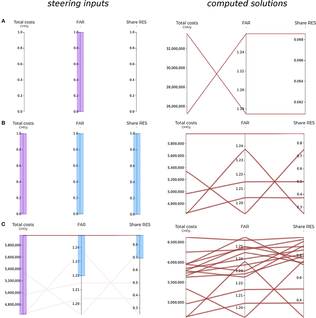
Figure 7. Parallel coordinates charts showing different steering inputs (left) and resulting solutions computed with Sobol sampling (right). (A) Set min and max objective on FAR to learn boundaries. (B) Request Pareto optimal solutions for all three axes. (C) Narrow the search for solutions in the upper parts of floor area ratio (FAR) and renewable energy sources (RES). Purple brushes indicates the primary objective in the ϵ-constraint formulation, and blue brushes indicate the range within which auxiliary constraints are varied.
A first question here is: can high shares of RES be achieved in a high density neighborhood? Having learned the bounds of achievable densities, they can dismiss them and continue to explore tradeoffs between solutions with densities between 1.17 and 1.27, RES shares between 0 and 100%, and minimal costs. This is performed by brushing an objective on the total costs axis, and specifying a range with Sobol sequence on the two other axes (Figure 7B).
As the solutions requested in Figure 7B appear, the user realizes after only 5 solutions that a satisfying RES share (0.88) is compatible with a high density (1.25), although at higher costs (5.97 MCHF/y). The question thus becomes: how much can the costs be reduced while maintaining an acceptable share of renewable energy and density? To answer this question, they brush new ranges on the upper parts of the floor area ration and renewable energy sources axes, to narrow the search only to those interesting areas, with the expectation to find a configuration which has a lower total cost than the currently most expensive solution (Figure 7C). A series of cheaper solutions appear, which the user can filter to reveal the tradeoffs with either FAR or RES that allowed the cost reduction. As visible in the right chart of Figure 7C, the Sobol sequence used to specify constraints guarantees a homogeneous and quick exploration of the areas of interest. As requested by the user, the sampling was first performed on the entire axes, then focuses on the upper areas, as denoted by more compact lines in the upper part of the FAR and RES axes.
Continuing this process, the user can answer further questions, such as: Which additional aspects explain the costs? Or: What energy technologies lead to these shares of renewable energy sources? For example, they might be interested in the remaining number of oil boilers in the proposed solutions, as a political target aims at decreasing their amount for environmental reasons.
By including the decentralized oil boiler axis via the drop-down menu (Figure 8A), they realize that still around 60 undesirable oil boilers are present in the neighborhood (red polylines in Figure 8A), which were initially present in the status quo. To assess the consequences of a drastic reduction in their number, they specify a constraint to prevent oil boilers in all upcoming solutions, while maintaining the exploration of cost-optimal solutions with both high density (>1.24) and high renewable energy share (>0.8). This generates ten new solutions with no oil boilers (blue polylines in Figure 8A).
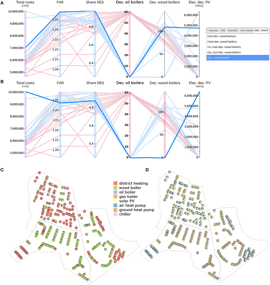
Figure 8. (A) Shows a highlighted polyline and the role each axis played in its problem formulation (purple–objective, blue–range, red–constraint), as well as the drop-down menu used to add axes. (B) Shows a different highlighted polyline, which is constrained on both fourth and fifth axes. Bold labels indicate the axes based on which a linear gradient coloring is performed. (C,D) Show the annual energy supply shares by technology per building for the solutions highlighted in (A,B) respectively.
The reduction in number of oil boilers has little effect on the total costs and performance of RES share compared to the solutions which included them. To explain this lack of effect, the user could further explore different criteria concerning the oil boilers and other technologies to find out their respective contributions to the neighborhoods energy supply. In this case however, a cartographic representation of the annual energy supply per building and per energy technology is more adapted to provide an overview of all technologies. The maps of solutions containing the oil boilers (not shown) are in fact similar to those without oil boilers (e.g., Figure 8C), with a predominance of district heating and wood boilers supplying the buildings. This indicates that oil boilers are only marginally used to satisfy peak loads, and can be substituted by the other installed technologies for only a limited cost increase.
Repeating this process for wood boilers, which are also to be avoided in urban centers because of health-related issues, the user adds a new constraint on the wood boiler axis, and requests five new solutions (Figure 8B). Note that in Figures 8A,B, the axes which influenced the generation of the highlighted polylines are colored accordingly, cf. section 2.3.3. The new constraint on wood boilers leads to a system dominated by solar PV panels and both ground and air source heat pumps. Furthermore, three of the five solutions were infeasible, indicating that shares of RES exceeding 0.88 become difficult to achieve without relying on wood boilers. Overall, the solutions without wood boilers are also more costly than the former solutions which relied on wood boilers and district heating (Figure 8B). The reason district heating is no longer chosen after adding the constraint on wood boilers (Figure 8D) is that the available centralized technologies used for the district heating do not allow to achieve the higher RES constraints. The inclusion in the model of e.g., deep geothermal or the nearby lake as heat sources could make district heating again a feasible solution for the current problem.
At this point, the user could continue by inquiring e.g., social or economic questions, such as the distribution of costs between building owners and energy provider, the impact of increased density on the view of aesthetic landmarks, etc. As the solution generation process evolves, however, the number of solutions and criteria rapidly grows. This is where MADA and cluster analysis can further support the exploration. To develop a general understanding of which solutions perform best, the TOPSIS method is applied on-the-fly to the current solutions, and colored accordingly (Figure 9A). Because the FAR axis is concentrated on a relatively tight range (1.19–1.26), the “max-min” normalization is adopted to ensure this criterion affects the final score equally to the other criteria (section 2.7.4). This “score” axis provides support to examine the best performing solutions, i.e., the solutions which are the most balanced, with respect to the TOPSIS indicator. For example, by displaying only the solutions with top scores, the user can assess whether (i) the solution reflects their preferences, and (ii) which tradeoffs are required for the improvement of any criterion. For illustration purposes, the score is computed here for only the first three axes, to allow also displaying it also in 3D scatter plots. These plots help to interpret the underlying concept of the TOPSIS approach (Figures 9B,C). Indeed, the geometrical distance between ideal solutions and actual solutions can more intuitively be grasped in the 3D charts than in parallel coordinates, although this visualization is limited to three axes.
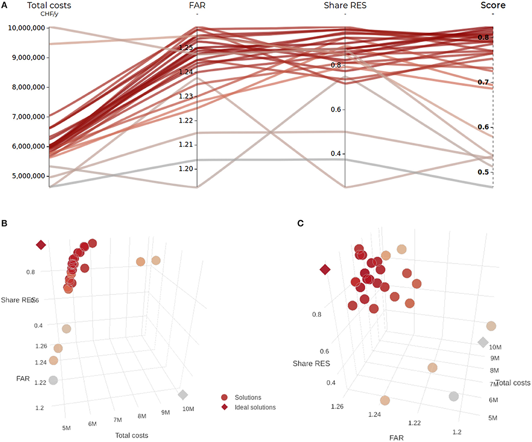
Figure 9. (A) Depiction of TOPSIS score results in parallel coordinates. (B) Lateral view of the Pareto surface in a 3D scatter plot. (C) Frontal view of the Pareto surface. Dark red solutions indicates solutions closest to the positive ideal.
Another way to cope with the many solutions is to perform cluster analysis to identify the few most representative solutions. In Figure 10, the user performed three cluster analyses for respectively k = 2, 3, 4 clusters. Depending on the number of solutions for which they are willing to spend time investigating in more detail, or depending on the quality of the clustering (either evaluated visually in the scatter plots or parallel coordinates or by relying on quality indices such as the silhouette index), a number of clusters—and their corresponding representative solutions (i.e., medoids)—are adopted. Figure 10D shows the clustering results for k = 3 clusters in parallel coordinates. The color reflects solutions which are part of a same cluster, and the thicker lines indicate the medoids for each cluster.
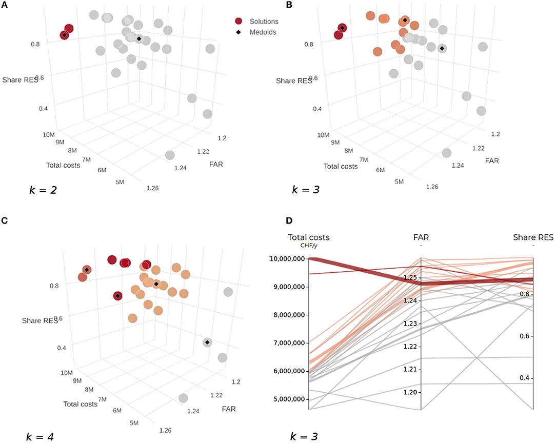
Figure 10. Depiction of the k-medoids cluster analysis results in 3D scatter plots for increasing number of clusters k. Colors indicate similar solutions belonging to a same cluster, and black diamonds indicate the representative solution (medoid) in each cluster. (A) Number of clusters is k = 2. (B) Number of clusters is k = 3. (C) Number of clusters is k = 4. (D) Alternate visualization of (B) with parallel coordinates chart (k = 3), where medoids are denoted by thicker lines.
3.4. Synthesis
After generating and exploring several alternatives, the user can narrow down the number of solutions to only a subselection of the most promising ones and add them to the comparer dashboard (Figure 11). They select seven axes, including a new criterion (“Share of performance certificates”) which indicates the share of buildings which were refurbished according to various energy performance standards. The cartographic thumbnails reflect this criterion, where lighter shades of red indicate buildings refurbished to stricter energy standards. From the 27 solutions generated so far, the three solutions which were added correspond to the three medoids of a cluster analysis performed on the chosen criteria. The first solution (ID 11) is the most cost effective (highlighted in green), but performs the least well in the five last indicators (highlighted in red). In the second solution (ID 10), the neighborhood is almost entirely supplied from renewable energy sources, but still relies on oil and wood boilers to satisfy part of the demand. Finally, the third solution (ID 27) is able to achieve 85% of renewable energy, in part by refurbishing 83% of the building stock, but nearly doubling the costs from the first solution.
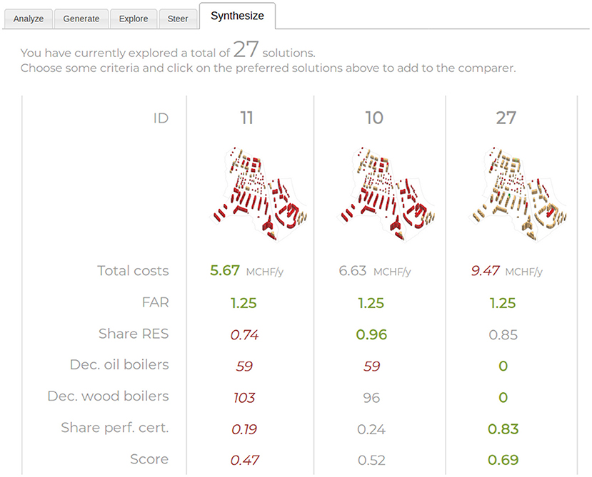
Figure 11. Comparer dashboard containing three representative solutions from a cluster analysis on the chosen criteria. The thumbnails depict the buildings in each solutions, colored by share of energy performance certificates (“Share perf. cert.”) adopted. Green fonts indicate the best performing values, red the worst.
3.5. Systematic Experience
By personally going through the systematic search process, the user has gained a better understanding of the problem and of their own preferences. New questions were raised along the way, which could be answered on-the-fly. The main learning points from this demonstration can be summarized as: knowledge of the maximum achievable density, required costs to achieve a highly renewable energy neighborhood, and the corresponding density threshold, as well as the maximum RES share achievable in the absence of wood boilers. Overall, this knowledge of extreme cases, but also the finer understanding of tradeoffs and tipping points between conflicting objectives gained during the search phase, give the user more confidence in justifying the chosen solutions, or the reasons why others were discarded. In addition, by laying down side-by-side the main criteria for a subselection of solutions in the synthesis phase, the user is equipped to take an informed decision, and justify and communicate it to other stakeholders.
4. Discussion
4.1. Strengths of the Approach
A novel interactive optimization methodology was presented, which enables users to simultaneously generate and explore solution spaces of large problems in real-time. It aimed at addressing the four main gaps in current interactive optimization methods, namely the ability to handle many objectives and alternatives, to explore the latter in an efficient way, to communicate the results effectively, and remain overall simple and accessible to users unfamiliar with optimization. Furthermore, it was demonstrated and applied in an urban system design problem. The contributions are summarized hereafter.
• Accessible: Parallel coordinates offer an effective framework for interactive optimization, as they provide a single entry point both for exploring a wide range of criteria and alternatives, while also offering an intuitive and natural way to specify preferences. By reducing the cognitive effort required from the user, the approach allows interactive optimization to benefit a wider audience. Indeed, the learning curve is essentially limited to understanding parallel coordinates, and not the technical aspects and jargon of optimization.
• Quick and efficient: The combined use of exact mathematical programming and quasi-random sampling offers an efficient approach to quickly explore large, multi-dimensional spaces. The real-time process allows the user to adapt the explored areas at any time, while building on the so-far acquired solutions.
• Improved parallel coordinates: While the main limitations of parallel coordinates such as cluttering and restriction to pairwise comparison of axes are well known and commonly addressed by means of brushing, line coloring and manual axes reordering, the present work extends traditional parallel coordinates in four ways. First, the traditional paradigm of parallel coordinates for exploring existing data is enhanced by the ability to dynamically populate the chart with desirable solutions. Second, a searchable axis-selection menu is appended to the chart to dynamically customize the visible axes. This allows to work with hundreds of criteria, by dynamically toggling the visibility of axes as initial questions are answered and new ones emerge. Third, cluster analysis can be performed interactively in order to focus the attention of the user on the most distinct solutions. Fourth, linked views allow to explore the entire data set as 3D scatter plots, while individual solutions can be explored beyond the purely quantitative nature of data in parallel coordinates. In this paper, cartographic maps were used, but the generation of other types of visualization (images, flowcharts, time-series…) could be linked to polylines in a similar way.
• Multiattribute and multiobjective decision analysis: The complementary strengths of MODA and MADA are harnessed to provide the user with a value-focused approach in generating good alternatives, while also providing them with assistance in ranking and selecting the best performing ones.
4.2. Limitations and Outlooks
• Different scalarization functions: While the ϵ-constraint method was favored for the reasons discussed above, it could nevertheless be interesting to explore other methods. For example, Cohon (1978, p. 157) noted that a potentially useful by-product of the weighted sum method is the weights themselves. It could be interesting and insightful to inform the user of the implicit objective weightings which lead to their preference for a solution.
• Multi-user usage: The assumption that there is only one user involved is often unrealistic, given that decision makers are typically either proxies influenced by and representing the interests of a larger group, or actually are a group (Zionts, 1994). While multi-user applications of the methodology have not been tested, the web interface and underlying data model have been designed with the intent of handling multiple users per project. Future research should thus investigate how the tool could be used either by multiple users in a same room (e.g., during interdisciplinary workshops) for consensus building, or by multiple users from remote locations. Some research has already been done in this area and provide useful starting points. Babbar-Sebens et al. (2015) studied multi-user applications of their interactive optimization tool. They proposed a “democratic” approach, in which the ratings of multiple users are aggregated into a common preference model, used to steer the search. Ferreira et al. (2006) also proposed a multi-user framework for the User Hints interactive optimization tool developed by do Nascimento and Eades (2005). They studied the effect of competition and cooperation in identifying new solutions, and proposed several mechanisms to share the best performing solutions from individual searches among a group of users. Various approaches could be envisaged for the use of parallel coordinates, such as highlighting lines which are most frequently requested by a group of users, recommending axes based on those which other users deemed important or allowing multiple users to interact with a same chart, jointly specifying ranges of interest.
• Improving parallel coordinate features: The presented methodology only exploited a few of the many possible functionalities for parallel coordinates. Future work could involve and test:
i. smart ordering of axes, e.g., by exhaustive pairwise depiction (Heinrich and Weiskopf, 2013), by conflicting objectives, prioritizing those with most convex Pareto fronts (Unal et al., 2017), by similarity-based reordering (Lu et al., 2016), by use of 3D parallel coordinates (Johansson and Forsell, 2016), or by visual (Keeney, 1992, p. 57) or automatic dimensionality reduction techniques (Copado-Méndez et al., 2016),
ii. improved visualization of polylines and patterns, e.g., visually bundling clusters into compact polygons (Palmas et al., 2014), or using polynomial curves and other line styles to emphasize various data properties (Franken, 2009; Heinrich and Weiskopf, 2013),
iii. handling of time series, e.g., using the third dimension to display temporal evolutions (Gruendl et al., 2016), by plotting several time steps on adjacent axes (Franken, 2009) or by animating a series of charts for each time-step (Heinrich and Weiskopf, 2013),
iv. dynamic rescaling of axes, to allow brushing beyond the visible values (currently brushing beyond the visible axis requires manually editing the numerical brush bound in an ad hoc table).
• Criteria selection: While this work was essentially focused on the proper generation of alternatives in the decision process, the identification of appropriate decision criteria is equally important (Keeney and Raiffa, 1976; León, 1999; Bond et al., 2008; Malczewski and Rinner, 2015). Keeney and Raiffa (1976) note in particular that two main properties of a decision criteria set are completeness and non-redundancy. Regarding completeness, the first applications of the methodology with urban planning practitioners revealed its potential in stimulating discussions and identifying missing criteria. Regarding non-redundancy, Keeney (1992, p. 57) points out that when objectives are explicitly listed and visualized, it becomes fairly easy to recognize redundancy, and parallel coordinates certainly help in this regard. The adoption of dimension reduction techniques as in Copado-Méndez et al. (2016) could furthermore also be applied in the future to provide the DM with a minimal set of non-redundant axes. However, it can be argued that redundancy is not necessarily to be avoided in the exploratory part of the methodology, as in some cases, the knowledge of how two redundant criteria correlate can be of interest.
• Expanding MADA: For demonstration purposes, only the TOPSIS method was implemented. Including various methods would let the user choose the method they are most comfortable with, or which is most relevant for their situation (Cajot et al., 2017a). For example, the weighted sum method might be preferable as more popular, while the outranking ELECTRE method or analytical hierarchy process might lead to more reliable results, at the expense of taking more time to elicit pairwise preference information from the user (Zanakis et al., 1998).
• Simplifying the steering process: Currently, the user still has specific control over the steering actions influencing the search. This makes sense in particular for an experienced user who aims to achieve specific outcomes. It is questionable whether a novice user actually requires such detailed control, and whether the distinction between objectives, ranges and constraints could be abolished (Wolf et al., 2009). Future work could explore a more complete automation of the steering process, in which regular “filter” brushes drawn by the user are automatically interpreted as steering actions, i.e., objectives and ranges. In this context, the Sobol sampling could be applied by default to all visible criteria to the largest known bounds, and the explored space is reduced as soon as the user applies a brush. The main limitations in this approach is that the user loses touch with the underlying mechanisms, and has less control over specific actions (e.g., set a constraint), which could potentially lead to wasted computational effort on less relevant solutions. Liu et al. (2018) argues that the interaction with the solver is key in building trust both in the model and the outcomes, and that the more opaque the approach, the greater the risk of non-acceptance and misunderstanding from the user.
• Machine learning: The fact that this methodology produces large amounts of data makes it well suited to exploit machine learning. Merkert et al. (2015) highlight three main contributions, which machine learning can bring to decision support systems: (i) higher effectiveness, (ii) efficiency and (iii) degree of automation. By learning from actions performed by the user (selected objectives, upper and lower bounds of brushes, axes toggled on or off, solutions added to the comparer dashboard, etc.), these could be at least partly automatized to support the user. Shneiderman (2010, p. 78) notes that “automation increases over time as procedures become more standardized and the pressure for productivity grows.” Arguably this can accelerate the process, avoid errors and reduce the user's cognitive effort. On the other hand, the benefits should be weighed against the risk of alienating the user from the process, hindering the trust they may have in the resulting solutions (Liu et al., 2018). Ultimately, the purpose of human-machine interaction is to best allocate tasks to each party according to their respective abilities. The fact that computers are increasingly outperforming humans in a growing number of tasks (e.g., image and pattern recognition) requires to rethink the role of the human in interactive methods, and how such methods are designed. A question is whether or not let the user perform some tasks for the sake of learning, even though the computer might do it better or faster than them.
5. Conclusion
5.1. Human-Machine Thinking
Whereas traditional interactive methods tend to clearly distinguish the learning phase, the preference articulation phase, and the generation of solutions, the proposed methodology blends these three phases into an integrated, more immersive experience. Indeed, the exploration of solutions need not be interrupted while the optimization is running: as soon as a solution is found, it is directly included into the chart—and into the user's mind—for the user to interpret. Through various exploratory features, the user becomes mindful of the relationships between criteria, and how much they are willing to sacrifice in one, in order to gain value in others. Each new solution makes more clear the critical contradictions to be resolved, allowing to refine the search toward areas which are found most relevant.
Because both the phases concerning the human and those concerning the computer occur at the same time, the whole can be considered an “optimization-based thought process.” The computer optimization becomes an extension of the user's mind, while at the same time, the user's mind becomes an extension of the optimization. Vinge (1993) anticipated the need for less “oracular” and more symmetrical decision support systems, where the program provides the user with as much information as the user provides the program guidance. He wrote that “computer/human interfaces may become so intimate that users may reasonably be considered superhumanly intelligent.” The direct and symmetrical link between human and computer offered by SAGESSE is a step in that direction.
5.2. A Source of Wisdom
Finally, the acronym of SAGESSE (French for wisdom) was chosen deliberately, as wisdom concerns “the ability to discern inner qualities and relationships” (Merriam-Webster dictionary, 1976), which is precisely what the methodology provides. It is our hope that the appealing nature of parallel coordinates and the powerful insights made possible by optimization, combined in the proposed methodology, will promote learning from even the most wicked problems. As the Greek philosopher Plato hinted (Republic, 2.376b), “is not the love of learning the love of wisdom, which is philosophy?”
Author Contributions
All authors listed have made a substantial, direct and intellectual contribution to the work, and approved it for publication.
Funding
The authors gratefully acknowledge the Canton of Geneva, as well as the European Commission for providing financial support during the conduct of research under the FP7-PEOPLE-2013 Marie Curie Initial Training Network CI-NERGY project with Grant Agreement Number 606851.
Conflict of Interest Statement
The authors declare that the research was conducted in the absence of any commercial or financial relationships that could be construed as a potential conflict of interest.
References
Aguirre, O., and Taboada, H. (2011). A Clustering Method Based on Dynamic Self Organizing Trees for Post-Pareto Optimality Analysis. Proc. Comput. Sci. 6, 195–200. doi: 10.1016/j.procs.2011.08.037
Akle, A. A., Minel, S., and Yannou, B. (2017). Information visualization for selection in Design by Shopping. Res. Eng. Design 28, 99–117. doi: 10.1007/s00163-016-0235-2
Allmendinger, R., Ehrgott, M., Gandibleux, X., Geiger, M. J., Klamroth, K., and Luque, M. (2016). Navigation in multiobjective optimization methods. J. Multi Criteria Decis. Anal. 24, 57–70. doi: 10.1002/mcda.1599
Ashour, Y., and Kolarevic, B. (2015). “Optimizing creatively in Multi-Objective Optimization,” in SimAUD '15 Proceedings of the Symposium on Simulation for Architecture & Urban Design, eds H. Samuelson, S. Bhooshan, and R. Goldstein (Washington, DC), 128–135.
Aydin, N., Mays, L., and Schmitt, T. (2014). Technical and environmental sustainability assessment of water distribution systems. Water Resour. Manag. 28, 4699–4713. doi: 10.1007/s11269-014-0768-y
Ayres, I., Raseman, S., and Shih, A. (2013). Evidence from two large field experiments that peer comparison feedback can reduce residential energy usage. J. Law Econ. Organ. 29, 992–1022. doi: 10.1093/jleo/ews020
Babbar-Sebens, M., Mukhopadhyay, S., Singh, V. B., and Piemonti, A. D. (2015). A web-based software tool for participatory optimization of conservation practices in watersheds. Environ. Model. Softw. 69, 111–127. doi: 10.1016/j.envsoft.2015.03.011
Bagajewicz, M., and Cabrera, E. (2003). Pareto optimal solutions visualization techniques for multiobjective design and upgrade of instrumentation networks. Indus. Eng. Chem. Res. 42, 5195–5203. doi: 10.1021/ie020865g
Balling, R., Taber, J., Brown, M., and Day, K. (1999). Multiobjective urban planning using genetic algorithm. J. Urban Plan. Develop. 125, 86–99. doi: 10.1061/(ASCE)0733-9488(1999)125:2(86)
Balling, R. J., Taber, J. T., Day, K., and Wilson, S. (2000). “City planning with a multiobjective genetic algorithm and a pareto set scanner,” in Evolutionary Design and Manufacture, ed I. C. Parmee (London: Springer), 237–247.
Bandaru, S., Ng, A. H. C., and Deb, K. (2017a). Data mining methods for knowledge discovery in multi-objective optimization: Part A - Survey. Expert Syst. Appli. 70, 139–159. doi: 10.1016/j.eswa.2016.10.015
Bandaru, S., Ng, A. H. C., and Deb, K. (2017b). Data mining methods for knowledge discovery in multi-objective optimization: Part B - New developments and applications. Expert Syst. Appli. 70, 119–138. doi: 10.1016/j.eswa.2016.10.016
Beach, L. R. (1993). Broadening the definition of decision making: the role of prechoice screening of options. Psychol. Sci. 4, 215–220.
Belton, V., Ackermann, F., and Shepherd, I. (1997). Integrated support from problem structuring through to alternative evaluation using cOPE and V·I·S·A. J. Multi Crit. Decis. Anal. 6, 115–130. 00184.
Belton, V., and Stewart, T. J. (2002). Multiple Criteria Decision Analysis. Boston, MA: Springer US.
Bond, S. D., Carlson, K. A., and Keeney, R. L. (2008). Generating objectives: can decision makers articulate what they want? Manag. Sci. 54, 56–70. doi: 10.1287/mnsc.1070.0754
Bostock, M., Ogievetsky, V., and Heer, J. (2011). D3: data-driven documents. IEEE Trans. Visual. Comput. Graph. 17, 2301–2309. doi: 10.1109/TVCG.2011.185
Branke, J., Deb, K., Miettinen, K., and Słowinski, R. (eds.). (2008). Multiobjective Optimization: Interactive and Evolutionary Approaches. Number 5252 in Lecture notes in computer science. Berlin: Springer.
Bratley, P., and Fox, B. L. (1988). Algorithm 659: implementing sobol's quasirandom sequence generator. ACM Trans. Math. Softw. 14, 88–100.
Buchanan, J. T. (1994). An experimental evaluation of Interactive MCDM methods and the decision making process. J. Operat. Res. Soc. 45, 1050–1059.
Buja, A., McDonald, J. A., Michalak, J., and Stuetzle, W. (1991). “Interactive Data Visualization Using Focusing and Linking,” in Proceedings of the 2Nd Conference on Visualization '91, VIS '91, (Los Alamitos, CA: IEEE Computer Society Press), 156–163.
Burhenne, S., Jacob, D., and Henze, G. P. (2011). “Sampling based on Sobol'sequences for Monte Carlo techniques applied to building simulations,” in Proceedings of International Conference on Building Performance Simulation Association (Sydney, NSW), 1816–1823.
Cajot, S., Mirakyan, A., Koch, A., and Maréchal, F. (2017a). Multicriteria decisions in Urban Energy System Planning: a review. Front. Ener. Res. 5:10. doi: 10.3389/fenrg.2017.00010
Cajot, S., Peter, M., Bahu, J.-M., Guignet, F., Koch, A., and Maréchal, F. (2017b). Obstacles in energy planning at the urban scale. Sustainable Cities and Society (From sustainable buildings to sustainable cities).
Cajot, S., Schüler, N., Peter, M., Koch, A., and Maréchal, F. (2017c). Interactive optimization for the planning of urban systems. Ener. Proc. 122, 445–450. doi: 10.1016/j.egypro.2017.07.383
Cajot, S., Schüler, N., Peter, M., Page, J., Koch, A., and Maréchal, F. (2016). “Establishing links for the planning of sustainable districts,” in Expanding Boundaries, eds G. Habert and A. Schlueter (Zurich: vdf Hochschulverlag AG an der ETH Zürich), 502–512.
Carli, R., Dotoli, M., Pellegrino, R., and Ranieri, L. (2017). A decision making technique to optimize a buildings #x2019; stock energy efficiency. IEEE Trans Syst. Man Cybern. Syst. 47, 794–807. doi: 10.1109/TSMC.2016.2521836
Chakraborty, S., and Yeh, C. H. (2009). “A simulation comparison of normalization procedures for TOPSIS,” in 2009 International Conference on Computers Industrial Engineering (Troyes), 1815–1820.
Chang, K. (2012). Parallel Coordinates-a Visual Oolkit for Multidimensional Detectives. Available online at: https://syntagmatic.github.io/parallel-coordinates/
Chankong, V., and Haimes, Y. Y. (2008). Multiobjective Decision Making: Theory and Methodology. New York, NY: Elsevier Science Publishing Co. Inc.
Chaudhari, P. M., Dharaskar, R. V., and Thakare, V. M. (2013). “Post pareto analysis in multi-objective Optimization,” in IJCA Proceedings on National Conference on Innovative Paradigms in Engineering & Technology 2013 (Nagpur), 15–18.
Chircop, K., and Zammit-Mangion, D. (2013). On e-constraint based methods for the generation of Pareto frontiers. J. Mech. Eng. Autom. 3, 279–289. Available online at: http://www.davidpublisher.org/index.php/Home/Article/index?id=3712.html
Cleveland, W. S., and McGill, R. (1985). Graphical perception and graphical methods for analyzing scientific data. Science 229, 828–833.
Collette, Y., and Siarry, P. (2004). Multiobjective Optimization: Principles and Case Studies. Berlin: Springer Verlag.
Copado-Méndez, P. J., Pozo, C., Guillén-Gosálbez, G., and Jiménez, L. (2016). Enhancing the ϵ-constraint method through the use of objective reduction and random sequences: Application to environmental problems. Comput. Chem. Eng. 87(Suppl. C), 36–48. doi: 10.1016/j.compchemeng.2015.12.016
deVries, B., Tabak, V., and Achten, H. (2005). Interactive urban design using integrated planning requirements control. Autom. Constr. 14, 207–213. doi: 10.1016/j.autcon.2004.07.006
do Nascimento, H. A. D., and Eades, P. (2005). User hints: a framework for interactive optimization. Future Generat. Comp. Syst. 21, 1177–1191. doi: 10.1016/j.future.2004.04.005
Feng, C.-M., and Lin, J.-J. (1999). Using a genetic algorithm to generate alternative sketch maps for urban planning. Comput. Environ. Urban Syst. 23, 91–108.
Ferreira, J. D. M., do Nascimento, H. A. D., and de Albuquerque, E. S. (2006). “Interactive optimization in cooperative environments,” in Proceedings of the 2006 Asia-Pacific Symposium on Information Visualisation-Vol. 60 (Tokyo: Australian Computer Society, Inc.), 117–120.
Fieldsend, J. E. (2016). Dynamic Visualisation of Many-Objective Populations. Portsmouth, VA: The Operational Research Society.
Fleming, P. J., Purshouse, R. C., and Lygoe, R. J. (2005). “Many-objective optimization: an engineering design perspective,” in Evolutionary Multi-Criterion Optimization, eds C. A. Coello, A. Arturo Hernández, and E. Zitzler (Berlin; Heidelberg: Springer), 14–32.
Fonseca, J. A., Nguyen, T.-A., Schlueter, A., and Marechal, F. (2016). City energy analyst (CEA): integrated framework for analysis and optimization of building energy systems in neighborhoods and city districts. Energy Build. 113, 202–226. doi: 10.1016/j.enbuild.2015.11.055
Franken, N. (2009). “Visual exploration of algorithm parameter space,” in 2009 IEEE Congress on Evolutionary Computation (Trondheim), 389–398.
French, S. (1984). Interactive Multi-objective programming: its aims, applications and demands. J. Operat. Res. Soc. 35, 827–834.
García-Cascales, M. S., and Lamata, M. T. (2012). On rank reversal and TOPSIS method. Math. Comput. Model. 56, 123–132. doi: 10.1016/j.mcm.2011.12.022
Gardiner, L. R., and Vanderpooten, D. (1997). “Interactive multiple criteria procedures: some reflections,” in Multicriteria Analysis, ed J. Clímaco (Berlin; Heidelberg: Springer), 290–301.
Gilbert, R. O. (1987). Statistical Methods for Environmental Pollution Monitoring. Technical Report PNL-4660, Pacific Northwest National Lab. (PNNL), Richland, WA.
Goy, S., Ashouri, A., Maréchal, F., and Finn, D. (2017). Estimating the potential for thermal load management in buildings at a large scale: overcoming challenges towards a replicable methodology. Ener. Proc. 111, 740–749. doi: 10.1016/j.egypro.2017.03.236
Greco, S., Ehrgott, M., and Figueira, J. R. (eds.). (2016). Multiple Criteria Decision Analysis, Vol. 233 of International Series in Operations Research & Management Science. (New York, NY: Springer).
Gruendl, H., Riehmann, P., Pausch, Y., and Froehlich, B. (2016). Time-series plots integrated in parallel-coordinates displays. Comput. Graph. Forum 35, 321–330. doi: 10.1111/cgf.12908
Haimes, Y. Y., Lasdon, L. S., and Wismer, D. A. (1971). On a bicriterion formulation of the problems of integrated system identification and system optimization. IEEE Trans. Syst. Man Cybern. SMC-1, 296–297.
Hakanen, J., Kawajiri, Y., Miettinen, K., and Biegler, L. T. (2007). Interactive multi-objective optimization for simulated moving bed processes. Control Cyber. 36, 283–302. Available online at: http://control.ibspan.waw.pl:3000/contents/show/4?year=2007
Hamel, S., Gaudreault, J., Quimper, C. G., Bouchard, M., and Marier, P. (2012). “Human-machine interaction for real-time linear optimization,” in 2012 IEEE International Conference on Systems, Man, and Cybernetics (SMC) (Seoul), 673–680.
Heinrich, J., and Weiskopf, D. (2013). “State of the art of parallel coordinates,” in Eurographics 2013 - State of the Art Reports, Vol. 2013 (Girona: The Eurographics Association), 95–116.
Hernández Gómez, R., Coello Coello, C. A., and Alba Torres, E. (2016). “A multi-objective evolutionary algorithm based on parallel coordinates,” in Proceedings of the Genetic and Evolutionary Computation Conference 2016 (ACM: New York, NY, USA.), 565–572.
Hwang, C.-L., and Masud, A. S. (1979). Multiple Objective Decision Making : Methods and Applications ; a State-of-the-Art Survey, Vol. 164 of Lecture notes in economics and mathematical systems. Berlin; Heidelberg: Springer-Verlag.
Hwang, C.-L., and Yoon, K. (1981). Multiple Attribute Decision Making: Methods and Applications. Berlin: Springer-Verlag.
Inselberg, A. (1985). The plane with parallel coordinates. Vis. Comput. 1, 69–91. doi: 10.1007/BF01898350
Inselberg, A. (1997). “Multidimensional detective,” in IEEE Symposium on Information Visualization 1997, Proceedings (Phoenix, AZ), 100–107.
Inselberg A. (2009). Parallel Coordinates: Visual Multidimensional Geometry and Its Applications. New York, NY: Springer.
Jaszkiewicz, A., and Słowiński, R. (1999). The ‘Light Beam Search' approach – an overview of methodology applications. Eur. J. Operat. Res. 113, 300–314.
Joe, S., and Kuo, F. Y. (2003). Remark on Algorithm 659: Implementing Sobol's Quasirandom Sequence Generator. ACM Trans. Math. Softw. 29, 49–57. doi: 10.1145/641876.641879
Johansson, J., and Forsell, C. (2016). Evaluation of parallel coordinates: overview, categorization and guidelines for future research. IEEE Trans. Visual. Comput. Graph. 22, 579–588. doi: 10.1109/TVCG.2015.2466992
Kaufman, L., and Rousseeuw, P. J. (2009). Finding Groups in Data: An Introduction to Cluster Analysis, Vol. 344. Hoboken, NJ: John Wiley & Sons.
Keeney, R. L. (1992). Value-Focused Thinking: A Path to Creative Decision Making. Cambridge: Harvard University Press.
Keeney, R. L., and Raiffa, H. (1976). Decisions With Multiple Objectives: Preferences and Value Trade-Offs. Cambridge: Cambridge University Press.
Kipouros, T., Mleczko, M., and Savill, M. (2008). “Use of parallel coordinates for post-analyses of multi-objective aerodynamic design optimisation in Turbomachinery,” in 4th AIAA Multidisciplinary Design Optimization Specialists Conference (Schaumburg, IL: American Institute of Aeronautics and Astronautics).
Klau, G. W., Lesh, N., Marks, J., and Mitzenmacher, M. (2010). Human-guided search. J. Heurist. 16, 289–310. doi: 10.1007/s10732-009-9107-5
Kok, M. (1986). The interface with decision makers and some experimental results in interactive multiple objective programming methods. Euro. J. Operat. Res. 26, 96–107.
Korhonen, P. (1996). “Reference direction approach to multiple objective linear programming: historical overview,” in Essays in Decision Making: A Volume in Honour of Stanley Zionts, eds M. Karwan, J. Spronk, and J. Wallenius (Berlin: Springer Verlag), 74–92.
Korhonen, P., and Yu, G. Y. (2000). “Quadratic pareto race,” in New Frontiers of Decision Making for the Information Technology Era, (World Scientific).
Larichev, O. I., Polyakov, O. A., and Nikiforov, A. D. (1987). Multicriterion linear programming problems: (analytical survey). J. Econ. Psychol. 8, 389–407.
Laukkanen, T., Tveit, T.-M., Ojalehto, V., Miettinen, K., and Fogelholm, C.-J. (2012). Bilevel heat exchanger network synthesis with an interactive multi-objective optimization method. Appl. Thermal Eng. 48, 301–316. doi: 10.1016/j.applthermaleng.2012.04.058
Laumanns, M., Thiele, L., and Zitzler, E. (2006). An efficient, adaptive parameter variation scheme for metaheuristics based on the epsilon-constraint method. Eur. J. Operat. Res. 169, 932–942. doi: 10.1016/j.ejor.2004.08.029
Lawler, E. L., and Wood, D. E. (1966). Branch-and-bound methods: a survey. Operat. Res. 14, 699–719.
León, O. G. (1999). Value-focused thinking versus alternative-focused thinking: effects on generation of objectives. Organ. Behav. Hum. Decis. Process. 80, 213–227.
Li, M., Zhen, L., and Yao, X. (2017). How to read many-objective solution sets in parallel coordinates. IEEE Comput. Intell. Mag. 12, 88–100. doi: 10.1109/MCI.2017.2742869
Liu, J., Dwyer, T., Marriott, K., Millar, J., and Haworth, A. (2018). Understanding the relationship between interactive optimisation and visual analytics in the context of prostate brachytherapy. IEEE Trans. Visual. Comput. Graph. 24, 319–329. doi: 10.1109/TVCG.2017.2744418
Lu, L. F., Huang, M. L., and Zhang, J. (2016). Two axes re-ordering methods in parallel coordinates plots. J. Vis. Lang. Comput. 33, 3–12. doi: 10.1016/j.jvlc.2015.12.001
Malczewski, J., and Rinner, C. (eds.). (2015). Multicriteria Decision Analysis in Geographic Information Science. New York, NY: Springer.
Martin, A. R., and Ward, M. O. (1995). “High dimensional brushing for interactive exploration of multivariate data,” in Proceedings of the 6th Conference on Visualization'95 (Atlanta, GA: IEEE Computer Society).
Mavrotas, G. (2009). Effective implementation of the ϵ-constraint method in multi-Objective Mathematical Programming problems. Appl. Math. Comput. 213, 455–465. doi: 10.1016/j.amc.2009.03.037
Meignan, D., Knust, S., Frayret, J.-M., Pesant, G., and Gaud, N. (2015). A review and taxonomy of interactive optimization methods in operations research. ACM Trans. Interact. Intell. Syst. 5:17. doi: 10.1145/2808234
Merkert, J., Mueller, M., and Hubl, M. (2015). “A survey of the application of machine learning in decision support systems,” in ECIS 2015 Completed Research Papers (Münster).
Merriam-Webster Dictionary (1976). Merriam-Webster's New Collegiate Dictionary. Colchester: The Book Service Ltd.
Miettinen, K. (2014). Survey of methods to visualize alternatives in multiple criteria decision making problems. OR Spectrum 36, 3–37. doi: 10.1007/s00291-012-0297-0
Miettinen, K., Eskelinen, P., Ruiz, F., and Luque, M. (2010). NAUTILUS method: an interactive technique in multiobjective optimization based on the nadir point. Euro. J. Operat. Res. 206, 426–434. doi: 10.1016/j.ejor.2010.02.041
Miettinen, K., and Kaario, K. (2003). Comparing graphic and symbolic classification in interactive multiobjective optimization. J. Multi Criter. Decis. Anal. 12, 321–335. doi: 10.1002/mcda.368
Miettinen, K., and Mäkelä, M. M. (2000). Interactive multiobjective optimization system WWW-NIMBUS on the Internet. Comput. Operat. Res. 27, 709–723. doi: 10.1016/S0305-0548(99)00115-X
Miller, G. A. (1956). The magical number seven, plus or minus two: some limits on our capacity for processing information. Psychol. Rev. 63:81.
Mokhtar, M., Burns, S., Ross, D., and Hunt, I. (2017). Exploring multi-objective trade-offs in the design space of a waste heat recovery system. Appl. Ener. 195(Suppl. C), 114–124. doi: 10.1016/j.apenergy.2017.03.030
Monz, M., Küfer, K. H., Bortfeld, T. R., and Thieke, C. (2008). Pareto navigation—algorithmic foundation of interactive multi-criteria IMRT planning. Phys. Med. Biol. 53:985. doi: 10.1088/0031-9155/53/4/0
Oberdieck, R., and Pistikopoulos, E. N. (2016). Multi-objective optimization with convex quadratic cost functions: a multi-parametric programming approach. Comput. Chem. Eng. 85, 36–39. doi: 10.1016/j.compchemeng.2015.10.011
Packham, I. S. J., Rafiq, M. Y., Borthwick, M. F., and Denham, S. L. (2005). Interactive visualisation for decision support and evaluation of robustness—in theory and in practice. Advan. Eng. Informat. 19, 263–280. doi: 10.1016/j.aei.2005.07.006
Palmas, G., Bachynskyi, M., Oulasvirta, A., Seidel, H. P., and Weinkauf, T. (2014). “An edge-bundling layout for interactive parallel coordinates,” in 2014 IEEE Pacific Visualization Symposium (Yokohama), 57–64.
Park, H.-S., and Jun, C.-H. (2009). A simple and fast algorithm for K-medoids clustering. Expert Syst. Appl. 36(2, Pt 2), 3336–3341. doi: 10.1016/j.eswa.2008.01.039
Piemonti, A. D., Babbar-Sebens, M., Mukhopadhyay, S., and Kleinberg, A. (2017a). Interactive genetic algorithm for user-centered design of distributed conservation practices in a watershed: an examination of user preferences in objective space and user behavior. Water Resour. Res. 53, 4303–4326. doi: 10.1002/2016WR019987
Piemonti, A. D., Macuga, K. L., and Babbar-Sebens, M. (2017b). Usability evaluation of an interactive decision support system for user-guided design of scenarios of watershed conservation practices. J. Hydroinformat. 19, 701–718. doi: 10.2166/hydro.2017.017
Pistikopoulos, E. N., Georgiadis, M. C., and Dua, V. (eds.). (2007). Multi-Parametric Programming, Vol. 1 of Process Systems Engineering. Weinheim: Wiley-VCH.
Plotly-Technologies-Inc. (2015). Collaborative Data Science. Available online at: https://plot.ly
Raphael, B. (2011). Multi-criteria decision making for collaborative design optimization of buildings. Built Environ. Proj. Asset Manag. 1, 122–136. doi: 10.1108/20441241111180398
Ribau, J., Sousa, J., and Silva, C. (2015). Reducing the carbon footprint of urban bus fleets using multi-objective optimization. Energy 93, 1089–1104. doi: 10.1016/j.energy.2015.09.112
Rosenberg, D. (2012). “Near-optimal water management to improve multi-objective decision making,” in 2012 Proceedings of iEMSs (Leipzig), 104–111.
Sato, H., Tomita, K., and Miyakawa, M. (2015). “Preferred region based evolutionary multi-objective optimization using parallel coordinates interface,” in 2015 3rd International Symposium on Computational and Business Intelligence (ISCBI) (Bali), 33–38.
Schüler, N., Agugiaro, G., Cajot, S., and Maréchal, F. (2018a). “Linking interactive optimization for urban planning with a semantic 3D city model,” in ISPRS Technical Commission IV Symposium 2018 (Delft).
Schüler, N., Cajot, S., Peter, M., Page, J., and Maréchal, F. (2018b). The optimum is not the goal: capturing the decision space for the planning of new neighborhoods. Front. Built. Environ. 3:76. doi: 10.3389/fbuil.2017.00076
Shenfield, A., Fleming, P. J., and Alkarouri, M. (2007). Computational steering of a multi-objective evolutionary algorithm for engineering design. Eng. Appl. Artif. Intell. 20, 1047–1057. doi: 10.1016/j.engappai.2007.01.005
Shin, W. S., and Ravindran, A. (1991). Interactive multiple objective optimization: survey I—continuous case. Comput. Operat. Res. 18, 97–114.
Shneiderman, B. (1996). “The eyes have it: a task by data type taxonomy for information visualizations,” in In Ieee Symposium on Visual Languages (Boulder, CO), 336–343.
Shneiderman, B. (2010). Designing the User Interface: Strategies for Effective Human-Computer Interaction. Boston, MA: Pearson Education India.
Siebert, J., and Keeney, R. L. (2015). Creating more and better alternatives for decisions using objectives. Operat. Res. 63, 1144–1158. doi: 10.1287/opre.2015.1411
Sobol, I. M. (1967). On the distribution of points in a cube and the approximate evaluation of integrals. USSR Comput. Math. Math. Phys. 7, 86–112.
Spronk, J. (1981). Interactive Multiple Goal Programming: Applications to Financial Planning. Springer, International Series in Management Science Operations Research.
Stump, G., Lego, S., Yukish, M., Simpson, T. W., and Donndelinger, J. A. (2009). Visual steering commands for trade space exploration: user-guided sampling with example. J. Comput. Inform. Sci. Eng. 9, 044501–044501–10. doi: 10.1115/1.3243633
Tanner, L. (1991). Selecting a text-processing system as a qualitative multiple criteria problem. Eur. J. Operat. Res. 50, 179–187.
Trutnevyte, E., Stauffacher, M., and Scholz, R. W. (2011). Supporting energy initiatives in small communities by linking visions with energy scenarios and multi-criteria assessment. Ener. Policy 39, 7884–7895. doi: 10.1016/j.enpol.2011.09.038
Unal, M., Warn, G. P., and Simpson, T. W. (2017). Quantifying the shape of pareto fronts during multi-objective trade space exploration. J. Mech. Desig. 140:021402–13. doi: 10.1115/1.4038005
Vanderpooten, D. (1989). The interactive approach in MCDA: a technical framework and some basic conceptions. Math. Comput. Model. 12, 1213–1220.
Vinge, V. (1993). “Technological singularity,” in VISION-21 Symposium Sponsored by NASA Lewis Research Center and the Ohio Aerospace Institute (Cleveland: OH), 30–31.
Wierzbicki, A. P. (2010). “The need for and possible methods of objective ranking,” in Trends in Multiple Criteria Decision Analysis, number 142 in International Series in Operations Research & Management Science eds M. Ehrgott, J. R. Figueira, and S. Greco (Boston, MA: Springer), 37–56.
Wolf, D., Simpson, T. W., and Zhang, X. L. (2009). “A preliminary study of novice and expert users' decision-making procedures during visual trade space exploration,” in International 35th Design Automation Conference on Design Engineering Technical Conferences and Computers and Information in Engineering Conference, Vol. 5 (San Diego, CA: ASME), 1361–1371.
Xiao, N., Bennett, D. A., and Armstrong, M. P. (2007). Interactive evolutionary approaches to multiobjective spatial decision making: a synthetic review. Comput. Environ. Urban Syst. 31, 232–252. doi: 10.1016/j.compenvurbsys.2006.08.001
Zanakis, S. H., Solomon, A., Wishart, N., and Dublish, S. (1998). Multi-attribute decision making: a simulation comparison of select methods. Eur. J. Operat. Res. 107, 507–529.
Zhen, L., Li, M., Cheng, R., Peng, D., and Yao, X. (2017). “Adjusting parallel coordinates for investigating multi-objective search,” in Simulated Evolution and Learning, Lecture Notes in Computer Science, eds Y. Shi, K. C. Tan, M. Zhang, K. Tang, X. Li, Q. Zhang, Y. Tan, M. Middendorf, and Jin, Y (Cham: Springer), 224–235.
Zio, E., and Bazzo, R. (2012). “A comparison of methods for selecting preferred solutions in multiobjective decision making,” in Computational Intelligence Systems in Industrial Engineering, Number 6 in Atlantis Computational Intelligence Systems, ed C. Kahraman (Paris: Atlantis Press), 23–43.
Keywords: interactive optimization, parallel coordinates, MILP, MCDA, urban planning, multiobjective optimization, data visualization
Citation: Cajot S, Schüler N, Peter M, Koch A and Maréchal F (2019) Interactive Optimization With Parallel Coordinates: Exploring Multidimensional Spaces for Decision Support. Front. ICT 5:32. doi: 10.3389/fict.2018.00032
Received: 11 June 2018; Accepted: 18 December 2018;
Published: 14 January 2019.
Edited by:
Gerrit C. Van Der Veer, University of Twente, NetherlandsReviewed by:
Andrej Košir, University of Ljubljana, SloveniaGualtiero Volpe, Università di Genova, Italy
Copyright © 2019 Cajot, Schüler, Peter, Koch and Maréchal. This is an open-access article distributed under the terms of the Creative Commons Attribution License (CC BY). The use, distribution or reproduction in other forums is permitted, provided the original author(s) and the copyright owner(s) are credited and that the original publication in this journal is cited, in accordance with accepted academic practice. No use, distribution or reproduction is permitted which does not comply with these terms.
*Correspondence: Sébastien Cajot, sebastien.cajot@alumni.epfl.ch